Siting thousands of radio transmitter towers on terrains with billions of points

Abstract.

This paper presents a system that sites (finds optimal locations for) thousands of radio transmitter towers on terrains of up to two billion elevation posts. Applications include cellphone towers, camera systems, or even mitigating environmental visual nuisances. The transmitters and receivers may be situated above the terrain. The system has been parallelized with OpenMP to run on a multicore CPU.

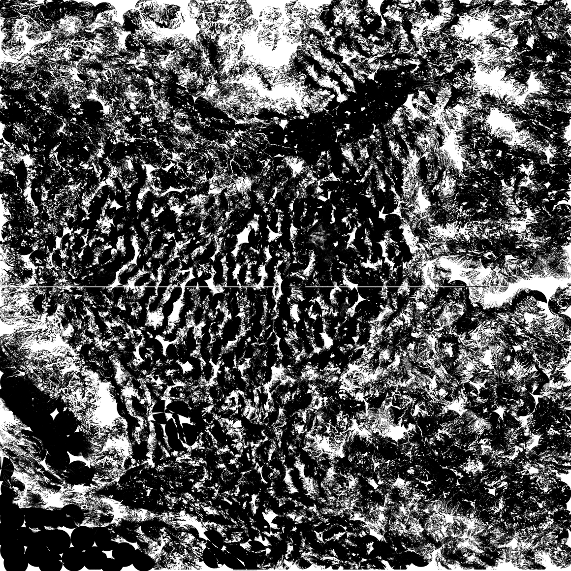
Cumulative viewsheds after siting observers on the US West data.

Figure 1. US West data ($46400\times 46400$ elevation posts); Cumulative viewsheds after siting 128, 512, 1024 and 4096 observers.

1. Definitions

Terrain::

a single valued function $z(x,y)$ describing a land or water surface, with $(x,y)$ varying over some domain, typically a square. The representation of this function will be discussed later.

Transmitter::

a 3D point $(t_{x},t_{y},t_{z})$ somewhere over the terrain; a source of straight-line radio or light waves. There may be thousands of transmitters.

Transmitter base::

$(t_{x},t_{y},z(t_{x},t_{y}))$ the point on the terrain directly below a transmitter.

Transmitter height::

$h_{t}$, the vertical distance between a transmitter and its base. Although this is not conceptually required, for simplicity, all the transmitters have the same height.

Radius of interest::

ROI, the maximum distance that a transmitter can transmit to. This is measured horizontally in 2D, not slantwise in 3D, and ignores possible differing elevations of the transmitter and receiver.

Receiver::

a 3D point $(r_{x},r_{y},r_{z})$ somewhere over the terrain, which is intended to receive a signal from a transmitter. Every point on the terrain within the ROI of a transmitter is a potential receiver.

Receiver height::

$h_{r}$, the vertical distance between a receiver and its base (the point on the terrain directly below it). Although this is not conceptually required, for simplicity, all the receivers have the same height, equal to the transmitter height.

Line of sight::

LOS, the straight line between a transmitter and receiver. The receiver is visible iff the LOS does not intersect the terrain. This work assumes that the radio wave travels in a straight line, ignoring diffraction and reflection off of the Heaviside layer in the upper atmosphere,

Viewshed::

a property of a transmitter $T$. A bitmap recording which of the potential receivers within the ROI of $T$ are visible from $T$.

Visibility index::

a property of a transmitter $T$. The fraction of the potential receivers within the ROI of $T$ that are visible. In other words, the normalized area of $T$’s viewshed.

DEM1000 terrain

Figure 2. DEM1000 terrain

Cumulative viewsheds for DEM1000

Figure 3. Cumulative viewsheds for DEM1000 after 1, 2, 4, 8, 16, 32, 64, 128, 256, 512, 1024, and 1264 transmitters sited

Table 1. DEM1000 test

Quantity	Value
Computer…
.. model	Xeon E-2276M
.. number of cores	6
.. number of hyperthreads	12
.. real memory	128 GB
.. nominal processor speed	2.8 GHz
Number of rows	1000
Number of columns	1000
Number of elevation posts	1 000 000
Min terrain elevation	6387
Max terrain elevation	16344
Transmitter height	10
Receiver height	10
Target coverage	95%
Radius of interest	30
Number of blocks the terrain divided into	100x100
Number of potential transmitters wanted per block	20
Total number of potential transmitters	200 000
Of those, number of transmitters selected	1264
Virtual memory used	142 GB
Real memory used	93 GB
Elapsed time (sec) to …
.. read data	0.025
.. compute estimated visibility indexes	0.056
.. find potential transmitters	0.013
.. compute their viewsheds	1.75
.. find the top transmitters	2.44
.. in total	4.30

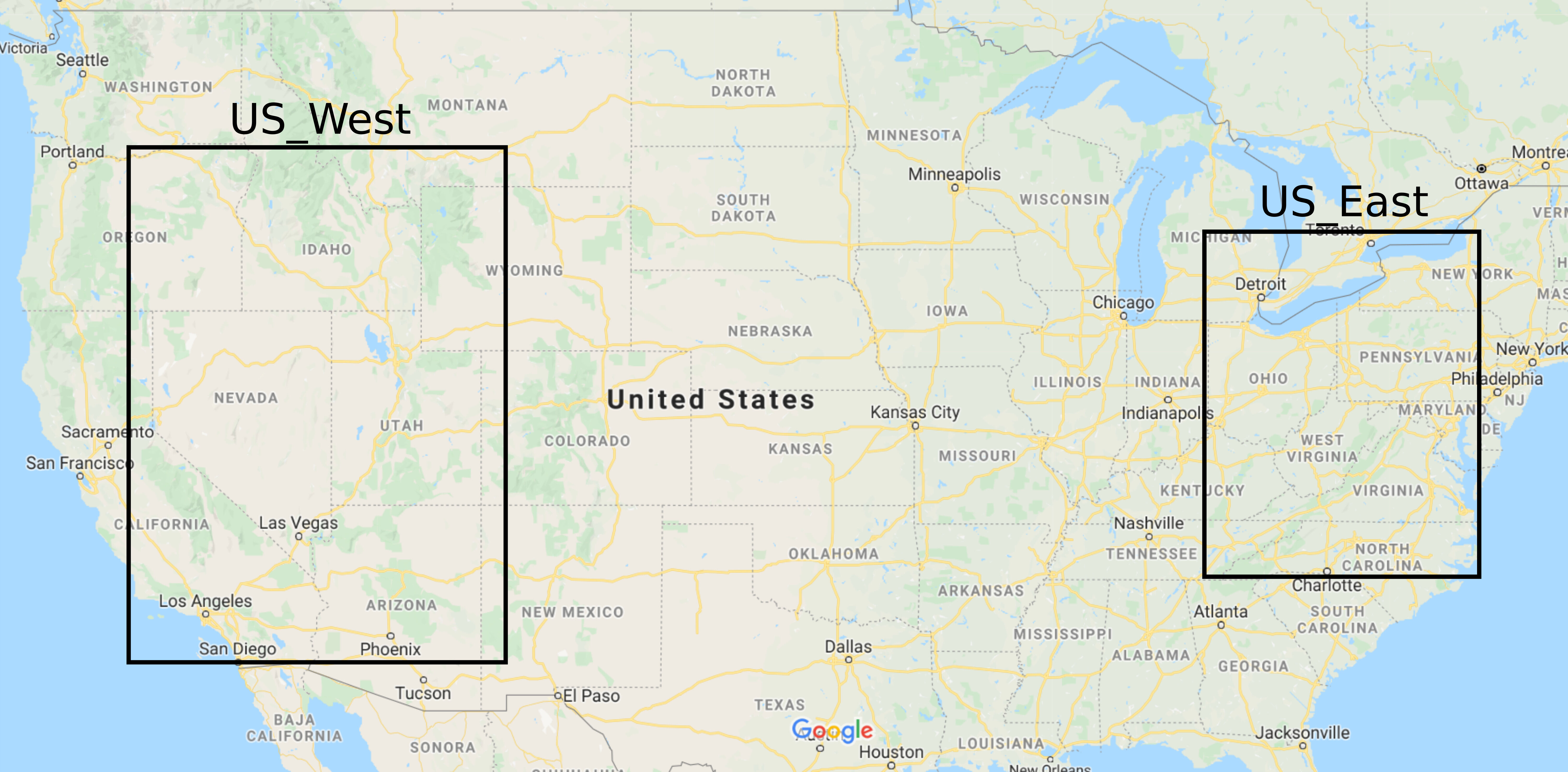
US West and East

Figure 4. US West and East dataset locations. Map data ©2020 Google.

US East

Figure 5. US East terrain

Table 2. US East tests

Quantity	Test 1 value	Test 2 value
Computer…
.. model	Xeon E-2276M
.. number of cores	6
.. number of hyperthreads	12
.. real memory	128 GB
.. nominal processor speed	2.8 GHz
Number of rows	32000
Number of columns	32000
Number of elevation posts	1 024 000 000
Min terrain elevation	7
Max terrain elevation	514
Transmitter height	100
Receiver height	10
Target coverage	95%
Radius of interest	500	1000
Number of blocks the terrain divided into	193x193	96x96
Number of potential transmitters wanted per block	20	20
Total number of potential transmitters	744 980	184 320
Of those, number of transmitters selected	6543	5000
Elapsed time (sec) to …
.. read data	24	22
.. compute estimated visibility indexes	149	188
.. find potential transmitters	14	14
.. compute their viewsheds	2145	2523
.. find the top transmitters	1501	1984
.. in total	3834	4732

2. Multiple transmitter siting

How should we best site (i.e., determine locations for) a set of radio transmitters $t_{i}$, to cover some terrain, so that the maximum number of receivers, $r_{j}$ can be accessed, or in other words, are visible?

The most important current application of this problem is in siting cell phone towers, and so this paper uses that terminology — transmitters, receivers, etc. However this problem is a few decades old, originally being of interest in the surveillance and environental visual domain. They use different a terminology of observers and targets. There we might have been siting a set of observers so that they could jointly see the most terrain. We even have wanted that the unsurveilled terrain consist of small separated regions instead of large connected regions that a smuggler might use. Mathematically, these are the same problem with different words.

3. Terrain representation

A formally grounded study of this problem would need a model for terrain. However, this important, and difficult, problem is not totally solved. It is hard because terrain has unusual properties.

1. Up and down are different for terrain. There are many sharp local maxima (peaks), but only few local minima (endorheic lakes), and they are broad, not sharp.

2. There are long-range monotonic features, aka river systems.

3. The many mostly smooth regions are interspersed with occasional discontinuities, aka cliffs.

This is important because those properties are not a good match for standard mathematical representations like Fourier series. In other engineering domains, such as signal processing, a function, perhaps the Fourier expansion

$$\sum_{k=0}^{N}a_{k}\cos kt+\sum_{k=1}^{N}b_{k}\sin kt$$

might be fitted to a sequence of sample points, and the physics of the problem will tend to match the math. That is, the mathematical operation of truncating the series at some $N$ to smooth out small features aligns with the physical operation of lo-pass filtering images or audio signals. This match does not apply to terrain.

Such a lo-pass filter would remove discontinuities like cliffs, which are, for many applications, the most important features of the terrain. Cliffs are visually recognizable, and affect mobility and drainage. The triangulated irregular triangle (TIN) representation also has this limitation.

Therefore, this paper will represent terrain with an equally spaced array of elevation posts, or a Digital Elevation Model. The DEM has its own limitations, but at least the representation is simple, and parallelization of the code is easier. “Equally spaced” is not possible over large regions. A bigger problem is what the elevation number at the post means. Here are some possibilities.

1. The reported elevation might be the terrain elevation at that precise point, to the extent possible. If the ideal terrain is $z(x,y)$ for real numbers $x$ and $y$, then $z_{ij}=z(x_{i},y_{j})$.

2. It might be a convolution or average over a region such as the region halfway to the next post. E.g.,

   $$z_{ij}=\int_{x_{i}-1/2}^{x_{i}+1/2}\int_{y_{j}-1/2}^{y_{j}+1/2}z(x,y)dxdy\ \ \ \ .$$

   A sinc function would be better than the above simple average since sinc goes to zero gradually instead of dropping off sharply.

3. The reported elevation might be the max elevation over the region, or some other function chosen to be useful to the desired application.

At this point, we have only the elevation array, and have no more information about the real terrain. However, we may need elevations at points between the elevation points. So we need an algorithm to interpolate elevations between adjacent posts. The particular problem here is deciding whether the terrain blocks a line of sight passing between adjacent two posts. There is no one best algorithm, since different applications have different needs. Isolated high elevations are of great interest to aviators. Cliffs affect land mobility. Monotonicity affects hydrography.

4. Terrain visibility

The terrain will be represented as an array of elevation posts $z_{ij}$. $i$ and $j$ can be considered to be $x$ and $y$ coordinates, respectively, if the elevation posts are 1 apart. We must determine whether transmitter $T$, whose 2D base is $(t_{x},t_{y})$, and whose 3D location is $(t_{x},t_{y},h_{t}+z_{t_{x},t_{y}})$ can see the receiver $R$, whose 2D base is $(r_{x},r_{y})$, and whose 3D location is $(r_{x},r_{y},h_{r}+z_{r_{x},r_{y}})$. This requires determining if a straight line, the LOS, drawn from $(t_{x},t_{y},h_{t}+z_{t_{x},t_{y}})$ to $(r_{x},r_{y},h_{r}+z_{r_{x},r_{y}})$ intersects the terrain. In general, the LOS runs between adjacent pairs of elevation posts, so we must interpolate elevations, in this case with a linear interpolation.

5. Prior art

Ray(Ray, 1994) and Franklin and Ray(Franklin and Ray, 1994a) described several fast programs to compute viewsheds and weighted visibility indices for observation points in a raster terrain. These programs explore various tradeoffs between speed and accuracy. They analyzed many cells of data; there is no strong correlation between a point’s elevation and its weighted visibility index. However, the, very few, high visibility points tend to characterize features of the terrain. Franklin(Franklin, 2002) presented an experimental study of a new algorithm that synthesizes separate programs, for fast viewshed, and for fast approximate visibility index determination, into a working testbed for siting multiple transmitters jointly to cover terrain from a full level-1 DEM, and to do it so quickly that multiple experiments are easily possible. Franklin and Vogt (Franklin and Vogt, 2004b, a, 2006) described two projects for siting multiple transmitters on terrain. Vogt(Vogt, 2004) studied the effect of varying the resolution.

A variation of this problem has recently been employed for siting a fixed number of terrestrial laser scanners on a terrain,  Starek et al. (2020). The authors employed a Simulated Annealing heuristic in their method, but focused only on very small instances with up to 6 transmitters on a $450\times 450$ terrain.

Tracy et al(Tracy et al., 2007), Tracy(Tracy, 2009), and Franklin et al(Franklin et al., 2007) extended multiple transmitter siting to compute smugglers paths to avoid the transmitters.

Andrade et al(Andrade et al., 2010) presented an external memory viewshed program, which managed paging the data better than the virtual memory manager (because it understood the data access pattern better). Magalhães et al(de Magalhães et al., 2011) and Ferreira et al(Ferreira et al., 2012, 2013, 2014a, 2016) improved the external memory algorithm and also presented a parallel viewshed algorithm in external memory. Pena et al(Pena et al., 2014a, b), Li(Li, 2016) and Li et al(Li et al., 2014; Li and Franklin, 2017) presented parallel observer siting algorithms running on GPUs.

It is also possible to consider receivers that have a certain quality, or are visible with some given probability, Akbarzadeh et al (Akbarzadeh et al., 2013). We might add constraints such as intervisibility, where transmitters are required to be visible from other transmitters. The transmitters and receivers might be mobile, Efrat (Efrat et al., 2012). Placing transmitters at different positions might have different costs.

The Modeling and Simulation community, which is disjoint from this community, discusses line-of-sight (with comparisons of various LOS algorithms) in US Army Topographic Engineering Center (2004), and the relation of visibility to topographic features, Lee (1992). Nagy (1994); Champion and Lavery (2002) studied line-of-sight on natural terrain defined by an $L_{1}$-spline.

The parallelization of line-of-sight and viewshed algorithms on terrains using GPGPU or multi-core CPUs is an active topic. Strnad (2011) parallelized the line-of-sight calculations between two sets of points—a source set and a destination set—on a GPU, and implemented it on a multi-core CPU for comparison. Zhao et al. (2013) parallelized Franklin’s R3 algorithm (Franklin and Ray, 1994b) to compute viewsheds on a GPU. The parallel algorithm combines coarse-scale and fine-scale domain decompositions to deal with memory limit and enhance memory access performance. Osterman (2012) parallelized the r.los module (R3 algorithm) of the open-source GRASS GIS on a GPU. Osterman et al. (2014) also parallelized Franklin’s R2 algorithm (Franklin and Ray, 1994b). Axell and Fridén (2015) parallelized and compared the R2 algorithm on a GPU and on a multi-core CPU. Bravo et al. (2015) parallelized Franklin’s XDRAW algorithm (Franklin and Ray, 1994b) to compute viewsheds on a multi-core CPU, after improving its IO efficiency and compatibility with SIMD instructions. Ferreira et al. (2014b, 2016) parallelized the sweep-line algorithm of Kreveld (1996) to compute viewsheds on multi-core CPUs. Qarah and Tu (Qarah and Tu, 2019) presented a fast GPU sweep-line viewshed algorithm, while Jianbo et al(Jianbo et al., 2019) used Spark. Wu et al(Wu et al., 2019) presented an interactive online multiple transmitter viewshed analysis system.

Rana (2003) proposed using topographic feature points, instead of random points, as receivers when estimating visibility indices. Wang et al. (2000) proposed a viewshed algorithm that uses a plane instead of lines of sight in each of 8 standard sectors around the transmitter to approximate the local horizon. The algorithm is faster but less accurate than XDRAW. Israelevitz (2003) extended XDRAW to increase accuracy by sacrificing speed. Wang and Dou(Wang and Dou, 2020) showed fast algorithm for filtering possible viewpoints. Eliş(Eliş, 2017) studied using multiple guard towers on terrain. Zhu et al(Zhu et al., 2019) improved XDRAW to remote chunk distortion. Lin et al(Lin et al., 2018) studied intervisibility.

Gillings(Gillings, 2015) used viewshed analysis in archeology. Shi and Xue(Shi and Xue, 2016) also minimized the number of transmitters while maximizing coverage. Prescott and Toma(Prescott and Toma, 2018) used a multiresolution approach. Yu et al(Yu et al., 2017) used a synthetic visual plane technique. Shrestha and Panday(Shrestha and Panday, 2017) improved on R3. Baek and Choi(Baek and Choi, 2018) compared different viewshed algorithms, using factors such as a 3D Fresnel zone. Efrat et al(Efrat et al., 2012) used visibility to pursue moving evaders.

US West

Figure 6. US West terrain.

Table 3. US West tests

Quantity	Test 1 value	Test 2 value
Computer…
.. model	Xeon E5-2660 v4
.. number of cores	14
.. number of hyperthreads	28
.. real memory	256 GB
.. nominal processor speed	2 GHz
Number of rows	46400
Number of columns	46400
Number of elevation posts	2 152 960 000
Min terrain elevation	80
Max terrain elevation	2786
Transmitter height	100
Receiver height	10
Target coverage	95%
Radius of interest	1000	2000
Number of blocks the terrain divided into	139x139	70x70
Number of potential transmitters wanted per block	20	20
Total number of potential transmitters	386420	98000
Of those, number of transmitters selected	5647	3347
Virtual memory used	195 GB
Real memory used	194 GB
Elapsed time (sec) to …
.. read data	118	109
.. compute estimated visibility indexes	130	143
.. find potential transmitters	9	8
.. compute their viewsheds	1706	2132
.. find the top transmitters	3510	3116
.. in total	5473	5509
CPU parallelism	32x

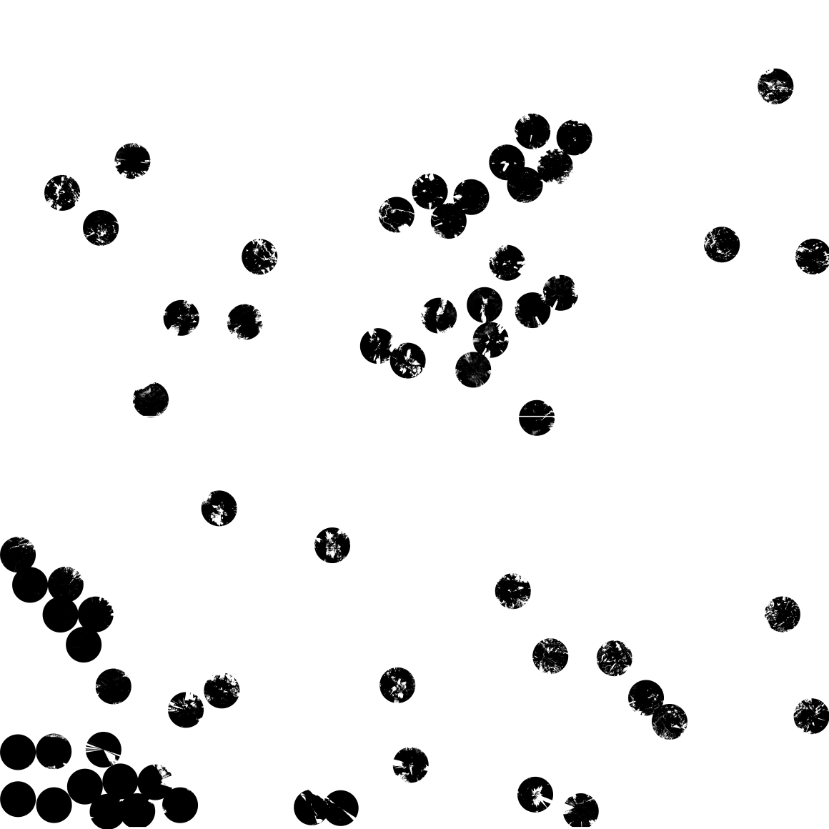
Cumulative viewsheds

Figure 7. Cumulative viewsheds for US West after 1, 2, 4, 8, 16, 32, 64, 128, 256, 1024, 2048, 4096, and 5647 transmitters sited

6. The multiple tranmitter siting process

This has four stages, summarized below. For more details, see Li and Franklin (2017).

Vix:

finds an approximate visibility index for each possible transmitter location in the terrain, using random sampling. For each location, i.e., each point in the map, 10 potential receiver locations are chosen uniformly randomly within a circle of radius ROI around the transmitter. Whether or not each one is visible is computed by testing whether the line of sight between them intersects the terrain. Extreme accuracy in computing these visible indexes is not required because their only use is to identify potential transmitters.

Findmax:

uses those visibility indices to compute a subset of of the potential transmitters, called top transmitters.

Merely sorting the potential transmitter list to select the first ones would be wrong. The problem is there might be a small high visibility region in the terrain. Inside this region there could be many transmitters, each with a high visibility index, but with largely overlapping viewsheds. So, they are redundant, but including them in the top list would crowd out lower visibility transmitters that are not redundant and would be useful to include in the solution.

Our solution is to partition the terrain into blocks of width ROI/3, and select the 20 transmitters in each block.

Viewshed:

computes the viewshed of each transmitter in the list returned by Findmax. It draws a circle of radius ROI around the transmitter and walks around it. For each point on the circle, it runs a line of sight from the transmitter. Then it walks along the line of sight, updating a horizon angle, to determine which points interior to the circle are visible. This process is linear time in the number of points in the circle, i.e., quadratic in the ROI.

The viewsheds are stored as bitmaps using 64-bit words.

Site:

is the heart of the process. Site greedily determines the set of actual top transmitters. It maintains a cumulative viewshed bitmap. At each step, it selects the transmitter, from the set returned by Findmax, whose viewshed would most increase the area of the cumulative viewshed when united with it. The union process is effected by bitwise operations on the 64-bit words, so it is fast.

Various optimizations are employed. E.g., in a later stage, a possible transmitter cannot increase the cumulative viewshed area by more than it would have increased it in an earlier stage.

This paper extends our earlier system to handle much larger datasets—up to two billion elevation posts.

7. Implementation

The above algorithm has been implemented in both serial and parallel versions, using C++ under Linux. The parallel versions use either OpenMP or CUDA. The program can run on a server or even on a good laptop, depending on the dataset size. The total virtual memory used to process one very large terrain was observed to be only 120 bytes per point, although this depends on factors such as the ROI. The time scales linearly with the relevant parameters, and has a small linear multiplicative factor. We consider our execution times to be fast enough that we are no longer really concerned with speed, but are testing the maximum feasible terrain size and studying various properties of the process. This paper’s experiments used OpenMP.

We use simple, regular, compact data structures, avoiding recursion, pointers, trees. This follows the Structure of Arrays paradigm. We avoid the $\log N$ factors in time or space that many other algorithms have; noting that here $N=2^{31}$. So our total storage is less, execution times small, and processing very large datasets is feasible.

More implementation details are as follows. OpenMP adds directives to the C++ program so that different iterations of a for loop can run in parallel. This assumes that the different iterations do not affect each other. E.g., they do not both write to the same variable. If that is required, then a critical directive can be used to serialize that access. The resulting program runs on a multicore Intel CPU. Our usual target machine is a dual 14-core Intel Xeon. The hard part of programming is designing the algorithm so that the code can be parallelized.

Defining parallel speedup of an algorithm is challenging. Elapsed real clock time is more useful than CPU time. A core that is not being used by this algorithm may well not be useful to another simultaneous program because other resources are constrained, such as I/O or memory. However Xeon CPUs can vary their clock speed over a range of sometime 3:1. They slow down when idle, but overclock and accelerate when running a compute-bound process. However, with current integrated circuit technology, the heat generated by a CPU varies with how hard it is computing. If all the CPU cores are being used, then it might overheat, and so it automatically slows down. This means that if a program uses all the cores intensively, they will slow down. So, even if the program is perfectly parallelizable, the real time speedup will be less than linear.

8. Testing

We used 3 test data sets.

8.1. DEM1000

This is a trivial test case with only 1,000,000 points; see Figure 2. Our laptop runs it in about 5 elapsed seconds, depending on the ROI. Nevertheless, it shows the richness of the cumulative viewsheds; see Figure 3. The stats for that test case are in Table 1.

8.2. US East

This dataset has over one billion points.

We generated some terrains using digital elevation models (with a 30-meter resolution) provided by the NASADEM dataset (Crippen et al., 2016). These data have been recently released by NASA and they were derived from elevations acquired by the Shuttle Radar Topography Mission (SRTM). One of the main advantages of these new models is that cells with missing elevation in the SRTM dataset (i.e., tagged with NODATA) have been filled.

Our US East dataset was extracted from the 1-arc-second NASADEM terrains, and is an example of a relatively flat region. It has $32,000\times 32,000=1\,024\,000\,000$ points. It bounds are 35N – 44N (a little less than 44), 85W – 76W. Figure 4 shows the locations of the US West and US East datasets. Figure 5 shows the US East terrain. Table 2 summarizes results from some tests on this data.

8.3. US West

Our largest test dataset, with over two billion points, is the US-West dataset extracted from the 1-arc-second NASADEM terrains. It has $46\,400\times 46\,400=2\,152\,960\,000$ points. It bounds are 33N – 46N (a little less than 46) , 121W – 108W; see Figure 6. It contains a nice mixture of flat and mountainous terrain.

Figure 7 shows how the cumulative viewshed progresses as more top transmitters are selected.

9. Summary and Future Work

We can process terrains with billions of points to site thousands of radio transmitter towers in $1\frac{1}{2}$ hours, or process terrains with merely a million points in a few seconds. Future work is to get the GPU code working on these large example, and experiment on the sensitivity of the result to lowered accuracy in the data.

References

- (1)
- Akbarzadeh et al. (2013) Vahab Akbarzadeh, Christian Gagné, Marc Parizeau, Meysam Argany, and Mir Abolfazl Mostafavi. 2013. Probabilistic Sensing Model for Sensor Placement Optimization Based on Line-of-Sight Coverage. IEEE Transactions on Instrumentation and Measurement 62, 2 (2013), 293–303.
- Andrade et al. (2010) Marcus V. A. Andrade, Salles V. G. de Magalhães, Mirella A. de Magalhães, W. Randolph Franklin, and Barbara M. Cutler. 2010. Efficient viewshed computation on terrain in external memory. Geoinformatica (2010). https://doi.org/10.1007/s10707-009-0100-9 (online 26 Nov 2009).
- Axell and Fridén (2015) Tobias Axell and Mattias Fridén. 2015. Comparison between GPU and parallel CPU optimizations in viewshed analysis. Master’s thesis. Chalmers University of Technology, Gothenburg, Sweden.
- Baek and Choi (2018) Jieun Baek and Yosoon Choi. 2018. Comparison of Communication Viewsheds Derived from High-Resolution Digital Surface Models Using Line-of-Sight, 2D Fresnel Zone, and 3D Fresnel Zone Analysis. ISPRS International Journal of Geo-Information 7, 8 (2018), 322.
- Bravo et al. (2015) Jesús Carabano Bravo, Tapani Sarjakoski, and Jan Westerholm. 2015. Efficient Implementation of a Fast Viewshed Algorithm on SIMD Architectures. In Proceedings of the 23rd Euromicro International Conference on Parallel, Distributed, and Network-Based Processing. (EUROMICRO, Sankt Augustin, Germany), Turku, Finland, 199–202.
- Champion and Lavery (2002) Danny C. Champion and John E. Lavery. 2002. Line of Sight in Natural Terrain Determined by -Spline and Conventional Methods. In 23rd Army Science Conference. Orlando, Florida.
- Crippen et al. (2016) R Crippen, S Buckley, E Belz, E Gurrola, S Hensley, M Kobrick, M Lavalle, J Martin, M Neumann, Q Nguyen, et al. 2016. NASADEM global elevation model: methods and progress. (2016).
- de Magalhães et al. (2011) Salles V. G. de Magalhães, Marcus V. A. Andrade, and W. Randolph Franklin. 2011. Multiple Observer Siting in Huge Terrains Stored in External Memory. International Journal of Computer Information Systems and Industrial Management (IJCISIM) 3 (2011).
- Efrat et al. (2012) Alon Efrat, Joseph S. B. Mitchell, Swaminathan Sankararaman, and Parrish Myers. 2012. Efficient Algorithms for Pursuing Moving Evaders in Terrains. In Proceedings of the 20th International Conference on Advances in Geographic Information Systems. (ACM, New York, New York), Redondo Beach, California, 33–42.
- Eliş (2017) Haluk Eliş. 2017. Terrain visibility and guarding problems. Ph.D. Dissertation. Bilkent University.
- Ferreira et al. (2016) Chaulio R. Ferreira, Marcus V. A. Andrade, Salles V. G. de Magalhães, and W. Randolph Franklin. 2016. An efficient external memory algorithm for terrain viewshed computation. ACM Trans. on Spatial Algorithms and Systems 2, 2 (2016). https://doi.org/10.1145/2903206
- Ferreira et al. (2013) Chaulio R. Ferreira, Marcus V. A. Andrade, Salles V. G. de Magalhães, W. R. Franklin, and Guilherme C. Pena. 2013. A Parallel Sweep Line Algorithm for Visibility Computation. In Geoinfo 2013, XIV Brazilian Symposium on GeoInformatics. Campos do Jordão, SP, Brazil. Winner of best paper award, http://www.geoinfo.info/geoinfo2013/index.php.
- Ferreira et al. (2014a) Chaulio R. Ferreira, Marcus V. A. Andrade, Salles V. G. de Magalhães, W. R. Franklin, and Guilherme C. Pena. 2014a. A parallel algorithm for viewshed computation on grid terrains. Journal of information and data management 5, 1 (2014). invited.
- Ferreira et al. (2014b) Chaulio R. Ferreira, Marcus V. A. Andrade, Salles V. G. Magalhães, W. Randolph Franklin, and Guilherme C. Pena. 2014b. A Parallel Algorithm for Viewshed Computation on Grid Terrains. Journal of Information and Data Management 5, 2 (2014), 171–180.
- Ferreira et al. (2012) Chaulio R. Ferreira, Salles V. G. de Magalhães, Marcus V. A. Andrade, W. Randolph Franklin, and André M. Pompermayer. 2012. More efficient terrain viewshed computation on massive datasets using external memory. In 20th ACM SIGSPATIAL International Conference on Advances in Geographic Information Systems (ACM SIGSPATIAL GIS 2012). Redondo Beach, CA.
- Franklin (2002) W. Randolph Franklin. 2002. Siting observers on terrain. In Advances in Spatial Data Handling: 10th International Symposium on Spatial Data Handling, Dianne Richardson and Peter van Oosterom (Eds.). Springer-Verlag, 109–120.
- Franklin et al. (2007) W Randolph Franklin, Metin Inanc, Zhongyi Xie, Daniel M. Tracy, Barbara Cutler, Marcus V A Andrade, and Franklin Luk. 2007. Smugglers and border guards – the GeoStar project at RPI. In 15th ACM International Symposium on Advances in Geographic Information Systems (ACM GIS 2007). Seattle, WA, USA.
- Franklin and Ray (1994a) Wm Randolph Franklin and Clark Ray. 1994a. Higher isn’t Necessarily Better: Visibility Algorithms and Experiments. In Advances in GIS Research: Sixth International Symposium on Spatial Data Handling, Thomas C. Waugh and Richard G. Healey (Eds.). The International Geographical Union’s Commission on Geographical Information Systems and The Association for Geographic Information, Taylor & Francis, Edinburgh, 751–770.
- Franklin and Ray (1994b) W. Randolph Franklin and Clark Ray. 1994b. Higher isn’t Necessarily Better: visibility Algorithms and Experiments. In Advances in GIS Research: Sixth International Symposium on Spatial Data Handling, Thomas C. Waugh and Richard G. Healey (Eds.). Taylor & Francis, Bristol, Pennsylvania, 751–770.
- Franklin and Vogt (2004a) W. Randolph Franklin and Christian Vogt. 2004a. Efficient observer siting on large terrain cells (extended abstract). In GIScience 2004: Third International Conference on Geographic Information Science. U Maryland College Park.
- Franklin and Vogt (2004b) W. Randolph Franklin and Christian Vogt. 2004b. Multiple observer siting on terrain with intervisibility or lo-res data. In XXth Congress, International Society for Photogrammetry and Remote Sensing. Istanbul.
- Franklin and Vogt (2006) W. Randolph Franklin and Christian Vogt. 2006. Tradeoffs when multiple observer siting on large terrain cells. In Progress in Spatial Data Handling: 12th International Symposium on Spatial Data Handling, Andreas Riedl, Wolfgang Kainz, and Gregory Elmes (Eds.). Springer, Vienna, 845–861. ISBN 978-3-540-35588-5.
- Gillings (2015) Mark Gillings. 2015. Mapping invisibility: GIS approaches to the analysis of hiding and seclusion. Journal of Archaeological Science 62 (2015), 1–14.
- Israelevitz (2003) David Israelevitz. 2003. A fast algorithm for approximate viewshed computation. Photogrammetric engineering and remote sensing 69, 7 (2003), 767–774.
- Jianbo et al. (2019) Zhang Jianbo, Chen Caikun, Liang Tingnan, Xia Hao, and Zhou Simin. 2019. A Parallel Implementation of an XDraw Viewshed Algorithm with Spark. In 2019 IEEE 21st International Conference on High Performance Computing and Communications; IEEE 17th International Conference on Smart City; IEEE 5th International Conference on Data Science and Systems (HPCC/SmartCity/DSS). IEEE, 19–28.
- Kreveld (1996) Marc Van Kreveld. 1996. Variations on Sweep Algorithms: efficient computation of extended viewsheds and class intervals. In Proceedings of the 7th International Symposium on Spatial Data Handling. (IGU Commission on GIS, Charleston, South Carolina), Delft, Netherlands, 15–27.
- Lee (1992) Jay Lee. 1992. Visibility Dominance and Topographic Features on Digital Elevation Models. In Proceedings 5th International Symposium on Spatial Data Handling, P. Bresnahan, E. Corwin, and D. Cowen (Eds.), Vol. 2. International Geographical Union, Commission on GIS, Humanities and Social Sciences Computing Lab, U. South Carolina, Columbia, South Carolina, USA, 622–631.
- Li (2016) Wenli Li. 2016. GPU-accelerated terrain processing. Ph.D. Dissertation. Rensselaer Polytechnic Institute.
- Li and Franklin (2017) Wenli Li and W. Randolph Franklin. 2017. GPU–Accelerated Multiple Observer Siting. Photogrammetric Engineering & Remote Sensing 83, 6 (June 2017), 439–446. https://doi.org/10.14358/PERS.83.6.439
- Li et al. (2014) Wenli Li, W. Randolph Franklin, Daniel N. Benedetti, and Salles V. G. de Magalhães. 2014. Parallel Multiple Observer Siting on Terrain. In 22nd ACM SIGSPATIAL International Conference on Advances in Geographic Information Systems (ACM SIGSPATIAL 2014). Dallas, Texas, USA.
- Lin et al. (2018) Menglong Lin, Chenbin Du, Xiang Cao, et al. 2018. An Improved Algorithm for Intervisibility Judgment Based on RSG. In 2018 5th International Conference on Information Science and Control Engineering (ICISCE). IEEE, 116–120.
- Nagy (1994) George Nagy. 1994. Terrain Visibility. Comput. & Graphics 18, 6 (1994).
- Osterman (2012) A. Osterman. 2012. Implementation of the r.cuda.los module in the open source GRASS GIS by using parallel computation on the NVIDIA CUDA graphic cards. Elektrotehniški Vestnik 79, 1–2 (2012), 19–24.
- Osterman et al. (2014) Andrej Osterman, Lucas Benedičič, and Patrik Ritoša. 2014. An IO-efficient Parallel Implementation of an R2 Viewshed Algorithm for Large Terrain Maps on a CUDA GPU. International Journal of Geographical Information Science 28, 11 (2014), 2304–2327.
- Pena et al. (2014b) Guilherme Pena, Salles de Magalhães, Marcus Andrade, Randolph Franklin, Chaulio Ferreira, Wenli Li, and Daniel Benedetti. 2014b. An efficient GPU multiple-observer siting method based on sparse-matrix multiplication. In 3rd ACM SIGSPATIAL International Workshop on Analytics for Big Geospatial Data (BigSpatial) 2014. Dallas TX USA.
- Pena et al. (2014a) Guilherme C. Pena, Marcus V.A. Andrade, Salles V.G. de Magalhães, W. R. Franklin, and Chaulio R. Ferreira. 2014a. An Improved Parallel Algorithm using GPU for Siting Observers on Terrain. In 16th International Conference on Enterprise Information Systems (ICEIS 2014). Lisbon, 367–375. https://doi.org/10.5220/0004884303670375
- Prescott and Toma (2018) Andrew Prescott and Laura Toma. 2018. A Multiresolution approach for viewsheds on 2D terrains. In Proceedings of the 26th ACM SIGSPATIAL International Conference on Advances in Geographic Information Systems. 63–72.
- Qarah and Tu (2019) Faisal F Qarah and Yi-Cheng Tu. 2019. A Fast Exact Viewshed Algorithm on GPU. In 2019 IEEE International Conference on Big Data (Big Data). IEEE, 3397–3405.
- Rana (2003) Sanjay Rana. 2003. Fast approximation of visibility dominance using topographic features as targets and the associated uncertainty. Photogrammetric Engineering and Remote Sensing 69, 8 (2003), 881–888.
- Ray (1994) Clark K. Ray. 1994. Representing Visibility for Siting Problems. Ph.D. Dissertation. Rensselaer Polytechnic Institute.
- Shi and Xue (2016) Xuan Shi and Bowei Xue. 2016. Deriving a minimum set of viewpoints for maximum coverage over any given digital elevation model data. International Journal of Digital Earth 9, 12 (2016), 1153–1167.
- Shrestha and Panday (2017) Subin Shrestha and Sanjeeb Prasad Panday. 2017. Faster Line of Sight Computation and Faster Viewshed Generation. In 2017 21st International Computer Science and Engineering Conference (ICSEC). IEEE, 1–5.
- Starek et al. (2020) Michael J Starek, Tianxing Chu, Helena Mitasova, and Russell S Harmon. 2020. Viewshed simulation and optimization for digital terrain modelling with terrestrial laser scanning. International Journal of Remote Sensing 41, 16 (2020), 6409–6426.
- Strnad (2011) Damjan Strnad. 2011. Parallel terrain visibility calculation on the graphics processing unit. Concurrency and Computation: Practice and Experience 23, 18 (2011), 2452–2462.
- Tracy (2009) Daniel M. Tracy. 2009. Path Planning and Slope Representation on Compressed Terrain. Ph.D. Dissertation. Rensselaer Polytechnic Institute.
- Tracy et al. (2007) Daniel M. Tracy, W. Randolph Franklin, Barbara Cutler, Marcus A Andrade, Franklin T Luk, Metin Inanc, and Zhongyi Xie. 2007. Multiple observer siting and path planning on lossily compressed terrain. In Proceedings of SPIE Vol. 6697 Advanced Signal Processing Algorithms, Architectures, and Implementations XVII. International Society for Optical Engineering, San Diego CA. paper 6697-16.
- US Army Topographic Engineering Center (2004) US Army Topographic Engineering Center (Ed.). 2004. Line of Sight Technical Working Group. http://www.tec.army.mil/operations/programs/LOS/.
- Vogt (2004) Christian Vogt. 2004. Siting Multiple Observers on Digital Elevation Maps of Various Resolutions. Master’s thesis. ECSE Dept., Rensselaer Polytechnic Institute.
- Wang et al. (2000) Jianjun Wang, Gary J. Robinson, and Kevin White. 2000. Generating viewsheds without using sightlines. Photogrammetric engineering and remote sensing 66, 1 (2000), 87–90.
- Wang and Dou (2020) Yiwen Wang and Wanfeng Dou. 2020. A fast candidate viewpoints filtering algorithm for multiple viewshed site planning. International Journal of Geographical Information Science 34, 3 (2020), 448–463.
- Wu et al. (2019) Ye Wu, Mengyu Ma, and Luo Chen. 2019. HiVewshed: An Interactive Online Viewshed Analysis System for Multiple Observers. In Proceedings of the 3rd International Conference on Computer Science and Application Engineering. 1–5.
- Yu et al. (2017) Jieqing Yu, Lixin Wu, Qingsong Hu, Zhigang Yan, and Shaoliang Zhang. 2017. A synthetic visual plane algorithm for visibility computation in consideration of accuracy and efficiency. Computers & Geosciences 109 (2017), 315–322.
- Zhao et al. (2013) Yanli Zhao, Anand Padmanabhan, and Shaowen Wang. 2013. A Parallel Computing Approach to Viewshed Analysis of Large Terrain Data Using Graphics Processing Units. International Journal of Geographical Information Science 27, 2 (2013), 363–384.
- Zhu et al. (2019) Guangyang Zhu, Jun Li, Jiangjiang Wu, Mengyu Ma, Li Wang, and Ning Jing. 2019. HiXDraw: An Improved XDraw Algorithm Free of Chunk Distortion. ISPRS International Journal of Geo-Information 8, 3 (2019), 153.