Nonlinear spectral synthesis of soliton gas in deep-water surface gravity waves

Abstract

Soliton gases represent large random soliton ensembles in physical systems that display integrable dynamics at the leading order. Despite significant theoretical developments and observational evidence of ubiquity of soliton gases in fluids and optical media their controlled experimental realization has been missing. We report the first controlled synthesis of a dense soliton gas in deep-water surface gravity waves using the tools of nonlinear spectral theory (inverse scattering transform (IST)) for the one-dimensional focusing nonlinear Schrödinger equation. The soliton gas is experimentally generated in a one-dimensional water tank where we demonstrate that we can control and measure the density of states, i. e. the probability density function parametrizing the soliton gas in the IST spectral phase space. Nonlinear spectral analysis of the generated hydrodynamic soliton gas reveals that the density of states slowly changes under the influence of perturbative higher-order effects that break the integrability of the wave dynamics.

Solitons are localized nonlinear waves that have been studied in many areas of science over last decades Remoissenet (1996); Kartashov et al. (2011); Dauxois and Peyrard (2006). Solitons represent fundamental nonlinear modes of physical systems described by a special class of wave equations of an integrable nature Zabusky and Kruskal (1965); Novikov et al. (1984); Yang (2010). These equations, like the Korteweg-de Vries (KdV) equation or the one-dimensional nonlinear Schrödinger equation (1D-NLSE), are of significant physical importance since they describe at the leading order the behavior of many systems in various fields of physics such as water waves, matter waves or electromagnetic waves Ablowitz et al. (1973); Remoissenet (1996); Dauxois and Peyrard (2006); Yang (2010); Trillo et al. (2016).

Nowadays the dynamics of soliton interaction is so well mastered that ordered sets of optical solitons or their periodic generalizations, the so-called finite-gap potentials, are synthesized and manipulated to carry out the transmission of information in fiber optics communication links Le et al. (2017); Turitsyn et al. (2017); Le et al. (2014); Kamalian et al. (2018). On the other hand, the question of collective dynamics of large random soliton ensembles represents a subject of active research in statistical mechanics and in nonlinear physics, most notably in the contexts of ocean wave dynamics and nonlinear optics, see e. g. ref. Osborne and Burch (1980); Osborne (1995); Onorato et al. (2001, 2013); Pelinovsky et al. (2008); Onorato et al. (2005); Hassaini and Mordant (2017); El Koussaifi et al. (2018); Randoux et al. (2014); Bromberg et al. (2010); Soto-Crespo et al. (2016); Dudley et al. (2014); Kraych et al. (2019).

The concept of soliton gas (SG) as a large ensemble of solitons randomly distributed in space and elastically interacting with each other originates from the work of Zakharov Zakharov (1971), who introduced kinetic equation for a non-equilibrium diluted gas of weakly interacting solitons of the KdV equation. The Zakharov’s kinetic equation has been generalised to the case of a dense SG in El (2003) (KdV) and in El and Kamchatnov (2005); El and Tovbis (2020) (focusing NLS). Each soliton in a gas living on the infinite line $x$ is characterised by a discrete eigenvalue $\lambda_{i}$ of the spectrum of the linear operator associated with the integrable evolution equation within the inverse scattering transform (IST) formalism. The fundamental property of integrable dynamics is the preservation of the soliton spectrum under evolution. The central concept in SG theory is the density of states (DOS) Lifshits et al. (1988) which represents the distribution $u(\lambda,x,t)$ over the spectral eigenvalues, so that $ud\lambda dx$ is the number of soliton states found at time $t$ in the element of the phase space $[\lambda,\lambda+d\lambda]\times[x,x+dx]$. The isospectrality of integrable dynamics results in the continuity equation $u_{t}+(us)_{x}=0$ for the DOS evolution in a spatially nonhomogeneous (non-equilibrium) SG. The transport velocity $s(\lambda,x,t)$ in the DOS continuity equation is different from the free soliton velocity due to position/phase shifts in pairwise soliton collisions, resulting in a non-local equation of state $s=\mathcal{F}[u]$, relating the transport velocity with the DOS El and Kamchatnov (2005); El and Tovbis (2020). Interestingly, the SG kinetic equation has recently attracted much attention in the context of generalized hydrodynamics for quantum many-body integrable systems, see Doyon et al. (2018a, b); Vu and Yoshimura (2019) and references therein.

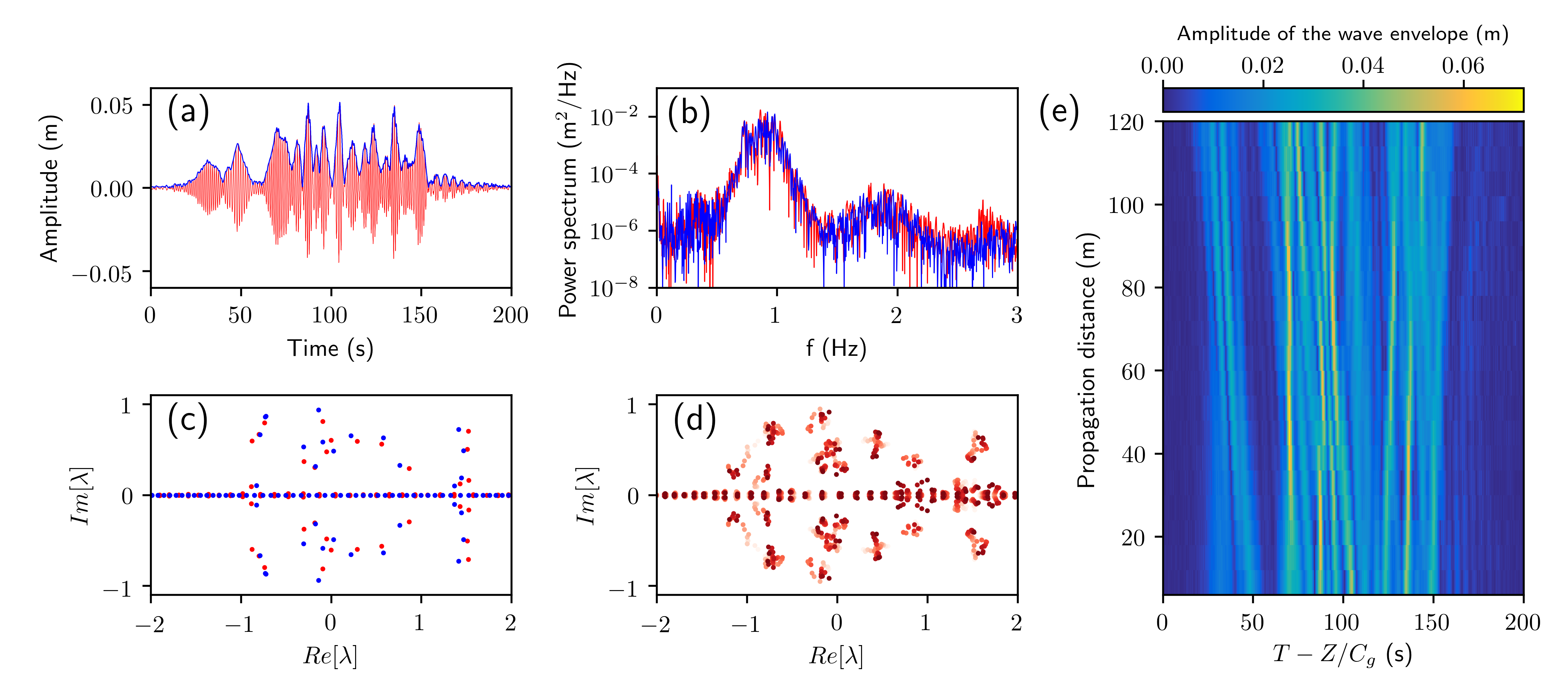
Figure 1: Ensemble of $N=16$ solitons propagating in the 1D water tank. (a) Water elevation (red line) and modulus of the wave envelope measured at $Z_{1}=6$ m, close to the wavemaker. (b) Fourier power spectra of wave elevation at $Z_{1}=6$ m (blue line) and at $Z_{20}=120$ m (red line). (c) Blue points represent the discrete IST spectrum of the numerically-generated N-SS $\psi_{16}(x,t=0)$ and red points represent the discrete IST spectrum measured at $Z_{1}=6$ m by using the signal plotted in (a). (d) Space evolution of the discrete IST spectra along the tank from $Z_{1}=6$ m (light red) to $Z_{20}=120$ m (dark red). (e) Space-time evolution of modulus of the wave envelope recorded by the $20$ gauges regularly spaced along the tank. Physical parameters characterizing the experiment are $f_{0}=0.9$ Hz, $k_{0}=3.26$ m^-1, $\alpha=0.895$, $L_{NL}=210$ m ($\langle|A_{0}(T)|^{2}\rangle=1.53\,\times 10^{-4}$ m²).

Despite various developments of SG theory (see e.g. Meiss and Horton Jr (1982); Fratalocchi et al. (2011); El et al. (2011); Dutykh and Pelinovsky (2014); Carbone et al. (2016); Shurgalina and Pelinovsky (2016); Girotti et al. (2018); Kachulin et al. (2020) ) and the existence of an unambiguous characterization of SG through the concept of DOS, the experimental/observational results in this area are quite limited. Costa et al have reported in 2014 the observation of random wavepackets in shallow water ocean waves that have been analyzed using numerical IST tools and interpreted as randomly distributed solitons that might be associated with KdV SG Costa et al. (2014). In 2015 large ensembles of interacting and colliding solitons have been observed in a levitating rectilinear water cylinder Perrard et al. (2015). In the recent experiments reported in ref. Redor et al. (2019), Redor et al have taken advantage of the process of fission of a sinusoidal wave train to generate an ensemble of bidirectional shallow water solitons in a $34$-m long flume. The interplay between multiple solitons and dispersive radiation has been analyzed by Fourier tranform and the observed random soliton ensemble has been interpreted as representing a SG. In optics, the SG terminology has been used to describe experiments where light pulses were synchronously injected in a passive optical fiber ring cavity Schwache and Mitschke (1997). Another recent experimental observation of complex nonlinear wave behavior attributed to SG dynamics was reported in Marcucci et al. (2019) where the formation of an incoherent optical field has been observed in the long-time evolution of a square pulse in a focusing medium El et al. (2016). However, in the absence of quantitative macroscopic (spectral) characterization the identification of the observed random wavefields with SG remains questionable. To our knowledge, there is no existing experiment where SG have been unambiguously identified using IST and where the measurement and control of the DOS of the SG have been achieved.

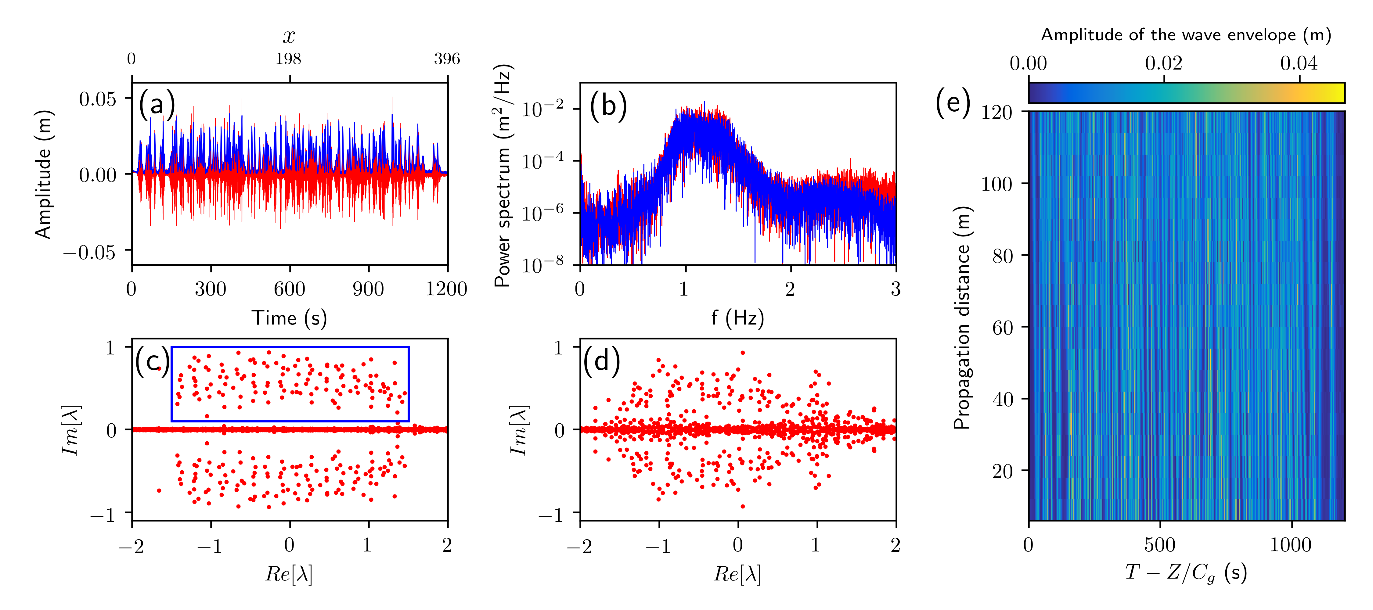
Figure 2: Gas of $N=128$ solitons propagating in the 1D water tank. (a) Water elevation (red line) and modulus of the wave envelope measured at $Z_{1}=6$ m, close to the wavemaker. (b) Fourier power spectra of wave elevation at $Z_{1}=6$ m (blue line) and at $Z_{20}=120$ m (red line). (c) Discrete IST spectrum measured at $Z_{1}=6$ m. (d) Discrete IST spectrum measured at $Z_{20}=120$ m. (e) Space-time evolution of modulus of the wave envelope recorded by the $20$ gauges regularly spaced along the tank. Physical parameters characterizing the experiment are $f_{0}=1.15$ Hz, $k_{0}=5.32$ m^-1, $\alpha=0.936$, $L_{NL}=45$ m ($\langle|A_{0}(T)|^{2}\rangle=1.58\,\times 10^{-4}$ m²).

In this Letter, we report experiments fully based on the IST method where we generate and observe the evolution of hydrodynamic deep-water dense soliton gases. We take advantage of the recently developed methodology for the effective numerical construction of the so-called $N$-soliton solutions of the focusing 1D-NLSE with $N$ large (ref. Gelash and Agafontsev (2018)), to create an incoherent wavefield having a dominant and controlled solitonic content characterized by a measurable DOS. We show that the generated SG may undergo some complex space-time evolution while the discrete IST spectrum is found to be nearly conserved, albeit being perturbed by higher-order effects.

Our experiments were performed in a wave flume $148$ m long, $5$ m wide and $3$ m deep. Unidirectional waves are generated at one end with a computer assisted flap-type wavemaker and the flume is equipped with an absorbing device strongly reducing wave reflection at the opposite end. As in the experiments reported in ref. Bonnefoy et al. (2020), the setup comprises $20$ equally spaced resistive wave gauges that are installed along the basin at distances $Z_{j}=6+(j-1)6$ m, $j=1,2,...20$ from the wavemaker located at $z=0$ m. This provides an effective measuring range of $114$ m.

In our experiment, the water elevation at the wavemaker reads $\eta(Z=0,T)=Re\left[A_{0}(T)e^{i\omega_{0}T}\right]$, where $\omega_{0}=2\pi f_{0}$ is the angular frequency of the carrier wave. $A_{0}(T)$ represents the complex envelope of the initial condition. Our experiments are performed in the deep-water regime, and they are designed in such a way that the observed dynamics is described at leading order by the focusing 1D-NLSE

$$\frac{\partial A}{\partial Z}+\frac{1}{C_{g}}\frac{\partial A}{\partial T}=i\frac{k_{0}}{\omega_{0}^{2}}\frac{\partial^{2}A}{\partial T^{2}}+i\alpha k_{0}^{3}|A|^{2}A,$$ (1)

where $A(Z,T)$ represents the complex envelope of the water wave that changes in space $Z$ and in time $T$ Osborne (2010). $k_{0}$ represents the wavenumber of the propagating wave ($\eta(Z,T)=Re\left[A(Z,T)e^{i(\omega_{0}T-k_{0}Z)}\right]$), which is linked to $\omega_{0}$ according to the deep water dispersion relation $\omega_{0}^{2}=k_{0}g$, where $g$ is the gravity acceleration. $C_{g}=g/(2\omega_{0})$ represents the group velocity of the wavepackets and $\alpha$ is a dimensionless term describing the small finite-depth correction to the cubic nonlinearity Bonnefoy et al. (2020).

The first important step of the experiment consists in generating an initial condition $A_{0}(T)$ in the form of a random wavefield having a pure solitonic content. To achieve this, we move to the “IST-friendly” canonical dimensionless form of the 1D-NLSE

$$i\frac{\partial\psi}{\partial t}+\frac{1}{2}\frac{\partial^{2}\psi}{\partial x^{2}}+|\psi|^{2}\psi=0,$$ (2)

where $\psi(x,t)$ represents the normalized complex envelope of the water wave. Connection between physical variables of Eq. (1) and dimensionless variables in Eq. (2) are given by $t=Z/L_{NL}$, $x=(T-Z/C_{g})\sqrt{g/(2L_{NL})}$ with the nonlinear length being defined as $L_{NL}=1/(\alpha k_{0}^{3}\langle|A_{0}(T)|^{2}\rangle)$, where the angle brackets denote average over time.

The nonlinear wavefield $\psi(x,t)$ satisfying Eq. (2) can be characterized by the so-called scattering data (the IST spectrum). For localized, i.e. decaying to zero as $|x|\rightarrow\infty$ wavefield the IST spectrum consists of a discrete part related to the soliton content and a continuous part related to the dispersive radiation. A special class of solutions, the $N$-soliton solutions (N-SS’s), exhibit only a discrete spectrum consisting of $N$ complex-valued eigenvalues $\lambda_{n}$, $n=1,...,N$ and $N$ complex parameters $C_{n}=|C_{n}|e^{i\phi_{n}}$, called norming constants, defined for each $\lambda_{n}$. In all the experiments described below, the phases $\phi_{n}$ of the norming constants $C_{n}$ characterizing the generated N-SS are randomly and uniformly distributed over $[0,2\pi)$ while their modulus $|C_{n}|$ are chosen to be equal to unity. As shown in ref. Gelash and Agafontsev (2018); Gelash et al. (2019), such $N$-soliton statistical ensemble is a good model for a homogeneous dense SG.

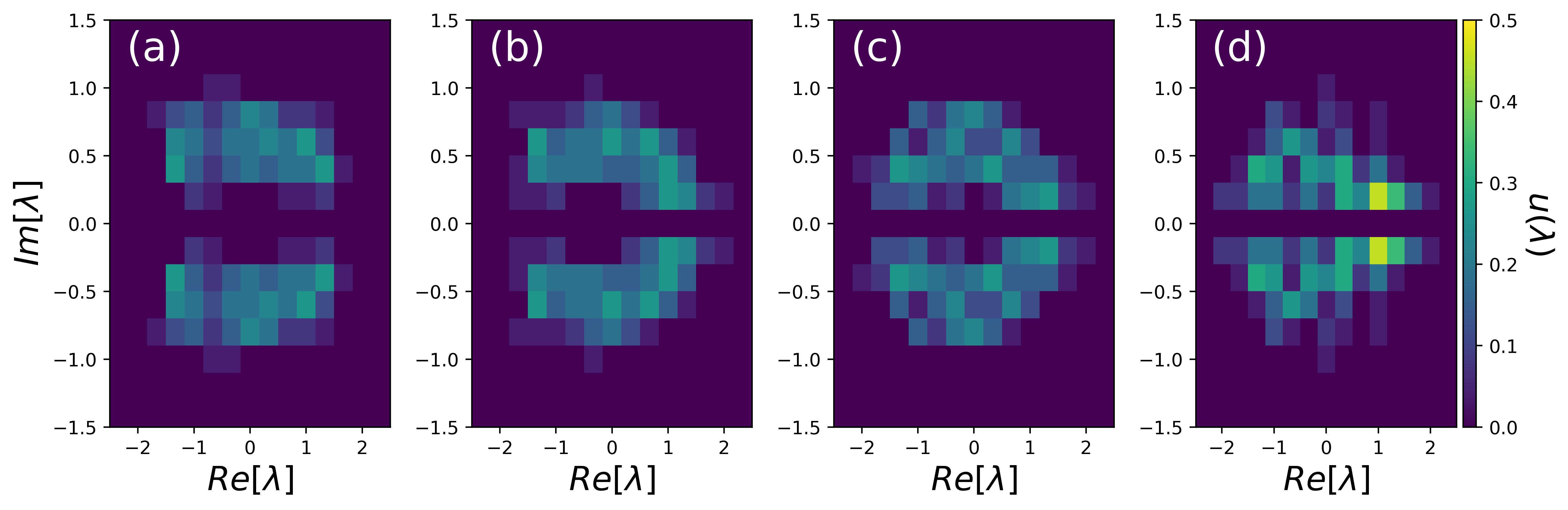
Figure 3: Statistical analysis of discrete IST spectra measured in Fig. 2 showing the slow evolution of the DOS $u(\lambda)$ (the probability density function of the discrete IST eigenvalues in the complex plane) as a function of propagation distance in the water tank: (a) $z_{1}=6$ m, (b) $z_{3}=18$ m, (c) $z_{10}=60$ m, (d) $z_{20}=120$ m.

In our first experimental run, we used numerical methods described in ref. Gelash and Agafontsev (2018) to generate a N-SS of Eq. (2) (see also Supplemental Material note_suppl ), hereafter denoted $\psi_{16}(x,t)$, with $N=16$ eigenvalues chosen arbitrarily within some domain of the complex spectral plane, as shown with blue points in Fig. 1(c). A relatively small number of solitons in this random soliton ensemble prevents its proper macroscopic spectral characterisation and the identification with SG. However, it is important as a first step in our experiment to establish a robust protocol for the generation of random soliton ensembles in a spectrally controlled way.

After some appropriate scaling, the generated dimensionless wavefield $\psi_{16}(x,t=0)$ is converted into the physical complex envelope $A_{16}(Z=0,T)=A_{0}(T)$ of the initial condition which is generated by the wavemaker. Fig. 1(a) shows the water elevation measured at $Z_{1}=6$ m together with the modulus of the envelope $|A_{16}(Z_{1},t)|$ computed using standard Hilbert transform techniques Osborne (2010). The generated wavefield with pure solitonic content spreads over approximately $140$ s and exhibits large amplitude fluctuations due to the random phase distribution. Fig. 1(c) shows the discrete IST spectrum that is computed from the signal recorded by the first gauge and plotted in Fig. 1(a). The measured eigenvalues plotted in red points in Fig. 1(c) are close to the discrete eigenvalues (blue points) that we have selected to build $\psi_{16}(x,t=0)$, the N-SS under consideration. This demonstrates that the process of generation of the N-SS solution is well controlled in our experiments.

As shown in Fig. 1(e), the space-time evolution of the generated wavepacket measured with $20$ gauges distributed along the tank reveals complex dynamics with multiple interacting coherent structures. At the same time, no significant broadening of the Fourier power spectrum of the wavefield is observed between $Z_{1}=6$ m and $Z_{20}=120$ m, as shown in Fig. 1(b). Despite the apparent complexity of the observed wave evolution, the measured discrete IST spectra, compiled and superimposed in Fig. 1(d), are nearly conserved over the whole propagation distance.

The fact that the isospectrality condition perfectly fullfilled in a numerical simulation of the 1D-NLSE (see Supplemental Material note_suppl ) is not exactly verified in the experiment arises from perturbative higher-order effects that break the integrability of the wave dynamics Chekhovskoy et al. (2019); Randoux et al. (2018); Bonnefoy et al. (2020), see Supplemental Material showing numerical simulations revealing the trajectories followed by eigenvalues in the complex spectral plane under the influence of higher-order effects note_suppl . In addition, the positions of the eigenvalues in Fig. 1(d) are also perturbed because of measurement inaccurracies. Nevertheless, the results of nonlinear spectral analysis reported in Fig. 1(d) show that the dynamical features observed for the wavefield composed of $16$ solitons are nearly integrable.

We now take advantage of the above method of the controlled generation of multiple-soliton, random phase solutions of the 1D-NLSE, to generate a random $N$-soliton ensemble that can be identified as SG. It is clear that to achieve that, the number of solitons $N$ should be sufficiently large. Fig. 2 shows the dynamical and spectral features characterizing the experimental evolution of an ensemble of $N=128$ solitons with random spectral (IST) characteristics. The important difference with the first example is that, due to a large number of solitons generated, we are now able to characterize the soliton ensemble by a DOS $u(\lambda)$, see Fig. 3. Specifically, we generate a SG with eigenvalues $\lambda_{i}\in\mathbb{C}$ distributed nearly uniformly on a rectangle in the upper half-plane of the complex IST spectral plane (and the c.c. rectangle in the lower half plane) and the DOS $u(\lambda)=u_{0}$ being nearly constant within the rectangle, see Fig. 2(c).

Fig. 2(a) shows that the generated SG has the form of a random wavefield spreading over $\Delta T=1200$ s which corresponds to a range $\Delta x=396$ in the dimensionless variables of Eq. (2). Clearly the generated SG does not represent a diluted SG composed of isolated and weakly interacting solitons but rather a dense SG which cannot be represented as superposition of individual solitons. Fig. 2(b) shows that the propagation of the generated SG is not accompanied by any significant broadening of Fourier power spectrum.

Fig. 2(c) shows the discrete IST spectrum of the wavefield measured at $Z_{1}=6$ m, close to the wavemaker. A set of $N=128$ eigenvalues is now measured within a rectangle in the upper complex plane. Similarly to the features reported in Fig. 1, the perturbative higher-order effects influence the observed dynamics and the discrete spectrum measured at $Z_{20}=120$ m is not identical to the one measured at $Z_{1}$, see Fig. 2(d). Even though the isospectrality condition characterizing a purely integrable dynamics is not exactly satisfied in our experiment, the measured discrete spectrum remains confined to a well-defined region of the complex plane. Moreover, the large number of eigenvalues distributed with some density within this limited region of the complex plane justifies the introduction of a statistical description of the spectral (IST) data, which represents the key point for the analysis of the observed wavefield in the framework of the SG theory.

In the context of the 1D-NLSE (2) the DOS $u(\lambda)$, where $\lambda=\beta+i\gamma$, represents the density of soliton states in the phase space i.e. $ud\beta d\gamma dx$ is the number of solitons contained in a portion of SG with the complex spectral parameter $\lambda\in[\beta,\beta+d\beta]\times[\gamma,\gamma+d\gamma]$ over the space interval $[x,x+dx]$ at time $t$ (corresponding to the position $Z$ in the tank). Considering that the generated SG is homogeneous in space, the DOS represents the probability density function of the complex-valued discrete eigenvalues normalised in such a way that $\int_{-\infty}^{+\infty}d\beta\int_{0}^{+\infty}d\gamma\,u(\lambda)=N/\Delta x$, where $N$ represents the number of eigenvalues found in the upper complex plane and $\Delta x$ represents the spatial extent of the gas. Fig. 3 displays the normalized DOS experimentally measured at different propagation distances in the water tank. We observe slow evolution of the DOS along the tank which is not due to gas’ nonhomegeneity but mainly originates from the presence of perturbative higher-order effects, see Supplemental Material including numerical simulations revealing an evolution of the DOS similar to the one illustrated in Fig. 3 note_suppl . Experimental results reported in Fig. 3 suggest that the incorporation of higher-order perturbative physical effects in the theory of SG represents a theoretical question of significant interest.

In this Letter, we have reported hydrodynamic experiments demonstrating that a controlled synthesis of a dense SG can be achieved in deep-water surface gravity waves. We show that the generated SG is characterized by a measurable spectral DOS, which provides an essential first step towards experimental verification of the kinetic theory of SGs. We hope that our work will stimulate new experimental and theoretical research in the fields of statistical mechanics and nonlinear random waves.

Supplemental Material for “Nonlinear spectral synthesis of soliton gases in deep-water surface gravity waves”

Pierre Suret,¹ Alexey Tikan,¹ Félicien Bonnefoy,² François Copie,¹ Guillaume Ducrozet,² Andrey Gelash,^3,4 Gaurav Prabhudesai,⁵ Guillaume Michel,⁶ Annette Cazaubiel,⁷ Eric Falcon,⁷ Gennady El,⁸ Stéphane Randoux¹

The purpose of this Supplemental Material is to provide some mathematical, numerical and experimental details that are utilized in the Letter. All equation, figure, reference numbers within this document are prepended with “S” to distinguish them from corresponding numbers in the Letter.

I Nonlinear spectral synthesis of N-soliton solutions of the focusing 1D-NLSE

In this section, we briefly describe the methodology used for the nonlinear synthesis of the large soliton ensembles propagating in the one-dimensional water tank. More theoretical details can be found in ref. Gelash and Agafontsev (2018).

We consider the focusing 1D-NLSE in the form

$$i\psi_{t}+\frac{1}{2}\psi_{xx}+|\psi|^{2}\psi=0\,,$$ (S1)

where $\psi(x,t)$ is a complex wave envelope varying in space $x$ and time $t$. In the IST method, the NLSE is represented as the compatibility condition of two linear equations Zakharov and Shabat (1972),

$$\Phi_{x}=\begin{pmatrix}-i\lambda&\psi\\ -\psi^{*}&i\lambda\\ \end{pmatrix}\Phi,$$ (S2)

$$\Phi_{t}=\begin{pmatrix}-i\lambda^{2}+\frac{i}{2}|\psi|^{2}&\frac{i}{2}\psi_{x}+2\lambda\psi\\ \frac{i}{2}\psi_{x}^{*}-\lambda\psi^{*}&i\lambda^{2}-\frac{i}{2}|\psi|^{2}\\ \end{pmatrix}\Phi,$$ (S3)

where $\lambda$ is a complex spectral parameter and $\Phi(t,x,\lambda)$ is a $2\times 2$ matrix wave function.

For spatially localized potentials $\psi$ such that $\psi(x,t)\rightarrow 0$ as $|x|\rightarrow\infty$, the eigenvalues $\lambda$ are presented by a finite number of discrete points with $\Im(\lambda)\neq 0$ (discrete spectrum) and the real line $\lambda\in\mathbb{R}$ (continuous spectrum). The scattering data consists of discrete eigenvalues $\lambda_{n}$, $n=1,...,N$ , norming constantss $C_{n}$ for each $\lambda_{n}$ and the so-called reflection coefficient $r(\xi)$,

$$\{r(\xi);\,\lambda_{n},\,C_{n}\}$$ (S4)

where $\xi$ means $\lambda$ on the real axis.

The simplest reflectionless ($r(\xi)=0$) solution of Eq. (S1) is the fundamental soliton which is parametrized by one discrete complex eigenvalue $\lambda_{1}$ and one associated complex norming constant $C_{1}$ that read

$$\lambda_{1}=-v_{1}/2+i\,a_{1}/2,\quad C_{1}=\exp i(\theta_{1}+2\lambda_{1}x_{1})$$ (S5)

With this setting the one-soliton solution of Eq. (S1) reads

$$\psi_{(1)}(x,t)=\frac{a_{1}\exp{\left[iv_{1}(x-x_{1})+\frac{i}{2}(a_{1}^{2}-v_{1}^{2})t+i\theta_{1}\right]}}{\cosh(a_{1}(x-x_{1})-a_{1}v_{1}t)}$$ (S6)

where $a_{1}>0$ represents the maximum amplitude of the soliton which moves with the group velocity $v_{1}$ in the $(x,t)$ plane. $x_{1}$ and $\theta_{1}$ represent the position and the phase of the soliton at $t=0$, respectively.

A special class of solutions of Eq. (S1), the N-soliton solution (N-SS), exhibits only a discrete spectrum ($r(\xi)=0$) consisting of N complex-valued eigenvalues $\lambda_{n}$, $n=1,...,N$ and their associated norming constants $C_{n}=|C_{n}|e^{i\phi_{n}}$. To construct a N-SS at the initial time $t=0$, we first generate an ensemble of $N$ discrete eigenvalues $\lambda_{n}=-v_{n}/2+i\,a_{n}/2$ and of their associated norming constants $C_{n}=\exp i(\theta_{n}+2\lambda_{n}x_{n})$. As discussed in details in ref. Gelash and Agafontsev (2018), the generation of the N-SS is achieved via a recurrent dressing procedure where discrete eigenvalues are iteratively added starting from the trivial solution $\psi_{(0)}=0$ of Eq. (S1).

The recurrence formula used to compute the N-SS is Gelash and Agafontsev (2018)

$$\psi_{(n)}(x,0)=\psi_{(n-1)}(x,0)+2i(\lambda_{n}-\lambda_{n}^{*})\frac{q_{n1}^{*}q_{n2}}{|q_{n}|^{2}},$$ (S7)

where the vector ${\bf q_{n}}=(q_{n1},q_{n2})^{T}$ is determined from ${\bf\Phi}_{n-1}$ and the scattering data of the ${\it n}$th soliton $\{\lambda_{n},\,C_{n}\}$, ${\bf q_{n}}(x)={\bf\Phi}_{n-1}^{*}(x,\lambda_{n}^{*})\left[\begin{array}[]{@{}c@{}}1\\ C_{n}\\ \end{array}\right]$. The corresponding solution ${\bf\Phi}_{n}(x,\lambda)$ of the Zakharov-Shabat system (S2) is calculated using ${\bf\Phi}_{n-1}$ and the so-called dressing matrix $\bm{\chi}$,

$$\bm{\Phi}_{(n)}(x,\lambda)=\bm{\chi}(x,\lambda).\bm{\Phi}_{(n-1)}(x,\lambda)$$ (S8)

$$\bm{\chi}_{ml}(x,\lambda)=\delta_{ml}+\frac{\lambda_{n}-\lambda_{n}^{*}}{\lambda-\lambda_{n}^{*}}\frac{q_{nm}^{*}q_{nl}}{|\bm{q_{n}}|^{2}}$$ (S9)

where $m,l=1,2$ and $\delta_{ml}$ is the Kronecker $\delta$ symbol Gelash and Agafontsev (2018).

II Inverse scattering transform analysis of the experimental data

In this Section, we describe briefly the method used to compute the discrete IST spectrum from the signals recorded in the water wave experiment.

The first step for performing the nonlinear analysis of the signals (water elevation given by $\eta(Z,T)=Re\left[A(Z,T)e^{i(k_{0}Z-\omega_{0}T)}\right]$) recorded in the experiments consists in determining the complex envelope $A(Z,T)$ of the wavefield. This is achieved by using standard techniques based on the Hilbert transform, as discussed e. g. in ref. Osborne (2010). Then, physical quantities are put to dimensionless form using the connection between physical and dimensionless variables that are provided in the Letter and recalled here for the sake of simplicity: $\psi=A/\sqrt{<|A_{0}(T)|^{2}>}$, $T=Z/L_{NL}$, $x=(T-Z/C_{g})\sqrt{g/(2L_{NL})}$ with the nonlinear length being defined as $L_{NL}=1/(\alpha k_{0}^{3}<|A_{0}(T)|^{2}>)$. The brackets denote average over time. Finally the IST discrete spectrum is determined by solving the Zakharov-Shabat system (S2) using the Fourier collocation method and following a procedure used and described in ref. Yang (2010); Randoux et al. (2016, 2018); Bonnefoy et al. (2020)

III Integrable versus non-integrable dynamics in the ensemble of 16 solitons

In this Section, we use numerical simulations of the focusing 1D-NLSE and of a modified (non-integrable) 1D-NLSE to show the role of higher order effects on the observed space-time dynamics and on the spectral (IST) features that characterize the evolution of the ensemble of $16$ solitons considered in Fig. 1 of the Letter.

Following the work reported in ref. Goullet and Choi (2011), higher-order effects in 1D water wave experiments can be described by a modified NLSE written under the form of a spatial evolution equation

$$\frac{\partial A}{\partial Z}=i\frac{k_{0}}{\omega_{0}^{2}}\frac{\partial^{2}A}{\partial T^{2}}+i\alpha k_{0}^{3}|A|^{2}A-\frac{k_{0}^{3}}{\omega_{0}}\left(6|A|^{2}\frac{\partial A}{\partial T}+2A\frac{\partial|A|^{2}}{\partial T}-2iA\mathcal{H}\left[\frac{\partial|A|^{2}}{\partial T}\right]\right),$$ (S10)

where $A(Z,T)$ represents the complex envelope of the wave field and $\mathcal{H}$ is the Hilbert transform defined by $\mathcal{H}[f]=(1/\pi)\int_{-\infty}^{+\infty}f(\xi)/(\xi-T)d\xi$. When the last three terms are neglected in Eq. (S10), the integrable 1D-NLSE is recovered.

Neglecting the last three terms in Eq. (S10), Fig. S1 shows results obtained from the numerical simulation of Eq. (S10) (integrable focusing 1D-NLSE) for the ensemble of $16$ solitons considered in the experiments reported in Fig. 1 of the Letter. Fig. S1(a) (resp. Fig. S1(b)) shows the modulus $|A(Z,T)|$ of the wavefield that is computed at $Z_{1}=6$ m (resp. at $Z_{20}=120$ m). Despite the significantly complicated space time evolution shown in Fig. S1(e) over the $120$ m-long propagation distance, the dynamics is integrable which implies that the discrete IST spectrum remains perfectly unchanged between $Z_{1}$ and $Z_{20}$, compare Fig. S1(c) and Fig.S1(d).

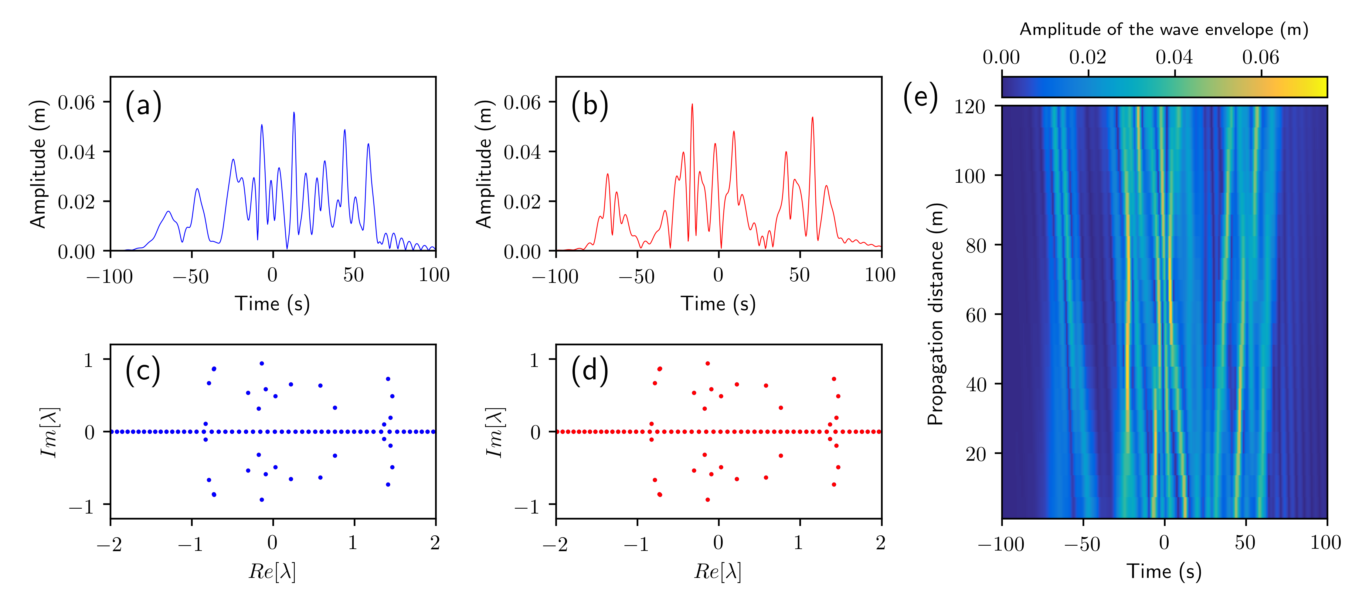
Figure S4: Integrable dynamics. Numerical simulations of the integrable focusing 1D-NLSE (Eq. (S10) where the last three terms are neglected) for the ensemble of $16$ solitons considered in Fig. 1 of the Letter. (a) Modulus $|A(Z_{1},T)|$ of the wave envelope at $Z_{1}=6$ m and (c) corresponding discrete IST spectrum. (b) Modulus $|A(Z_{20},t)|$ of the wave envelope at $Z_{20}=120$ m and (d) corresponding discrete IST spectrum. (e) Space-time plot showing the nonlinear evolution of the modulus $|A(Z,T)|$ of the wave envelope.

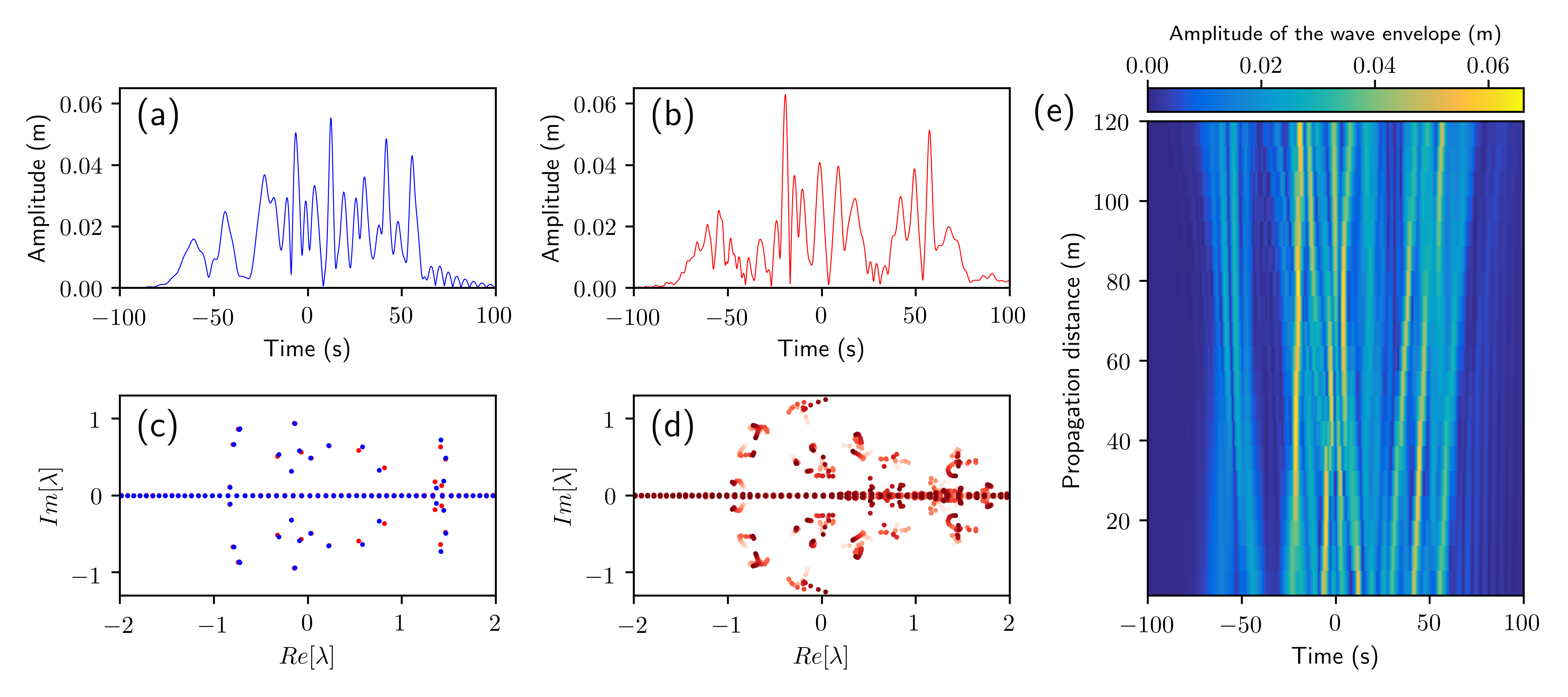
Figure S5: Non-integrable dynamics. Numerical simulations of Eq. (S10) for the ensemble of $16$ solitons considered in Fig. 1 of the Letter. (a) Modulus $|A(Z_{1},t)|$ of the wave envelope at $Z_{1}=6$ m and (c) corresponding discrete IST spectrum. (b) Modulus $|A(Z_{20},t)|$ of the wave envelope at $Z_{20}=120$ m . (d) Space evolution of the discrete IST spectra along the tank from $Z_{1}=6$ m (light red) to $Z_{20}=120$ m (dark red). (e) Space-time plot showing the nonlinear evolution of the modulus $|A(Z,T)|$ of the wave envelope.

If higher order effects described by the three last terms in Eq. (S10) are taken into account, the space-time evolution is slightly perturbed compared to the integrable case, compare Fig. S2(b) with Fig. S1(b) and Fig. S2(e) with Fig. S1(e). Contrary to results reported in Fig. S1, the isospectrality condition is now not verified because of the higher-order effects that break the integrability of the wave dynamics. Fig. S2(d) shows clearly that each of the $16$ discrete eigenvalues composing the random wavefield does not remain invariant over propagation distance but follows an individual trajectory in the complex plane, as already e.g. evidenced in ref. Chekhovskoy et al. (2019) in numerical simulations of a laser system. Similar spectral (IST) results have been presented in experimental results reported in Fig. 1 of the Letter. However clean trajectories in the complex IST plane cannot be clearly identified in experiments because of small calibration errors in the measurement of the wave elevation.

IV Influence of higher-order efects on the gas of $128$ solitons

In this Section, we show that Eq. (S10) describes well dynamical and statistical features reported in Fig. 2 and in Fig. 3 of the Letter for the gas of $128$ solitons.

Fig. S3 shows numerical simulations of Eq. (S10) that are made with physical values characterizing the experiments presented in the Letter for the gas of $128$ solitons. Dynamical and spectral features very similar to those reported in Fig. 2 of the Letter are found in numerical simulations reported in Fig. S3. In particular the isospectrally condition is not verified because of the perturbative higher order effects described by the last three terms in Eq. (S10). This results in discrete IST spectra that significantly change with propagation distance (compare Fig. S3(c) and Fig. S3(d)) even though they remain confined in a well defined region in the complex plane.

Fig. S4 shows the normalized density of states, i.e. the probability density function of the complex-valued discrete eigenvalues characterizing the SG over the time interval $\Delta T=1200$ s It is determined at different propagation distances from numerical simulations of Eq. (S10).

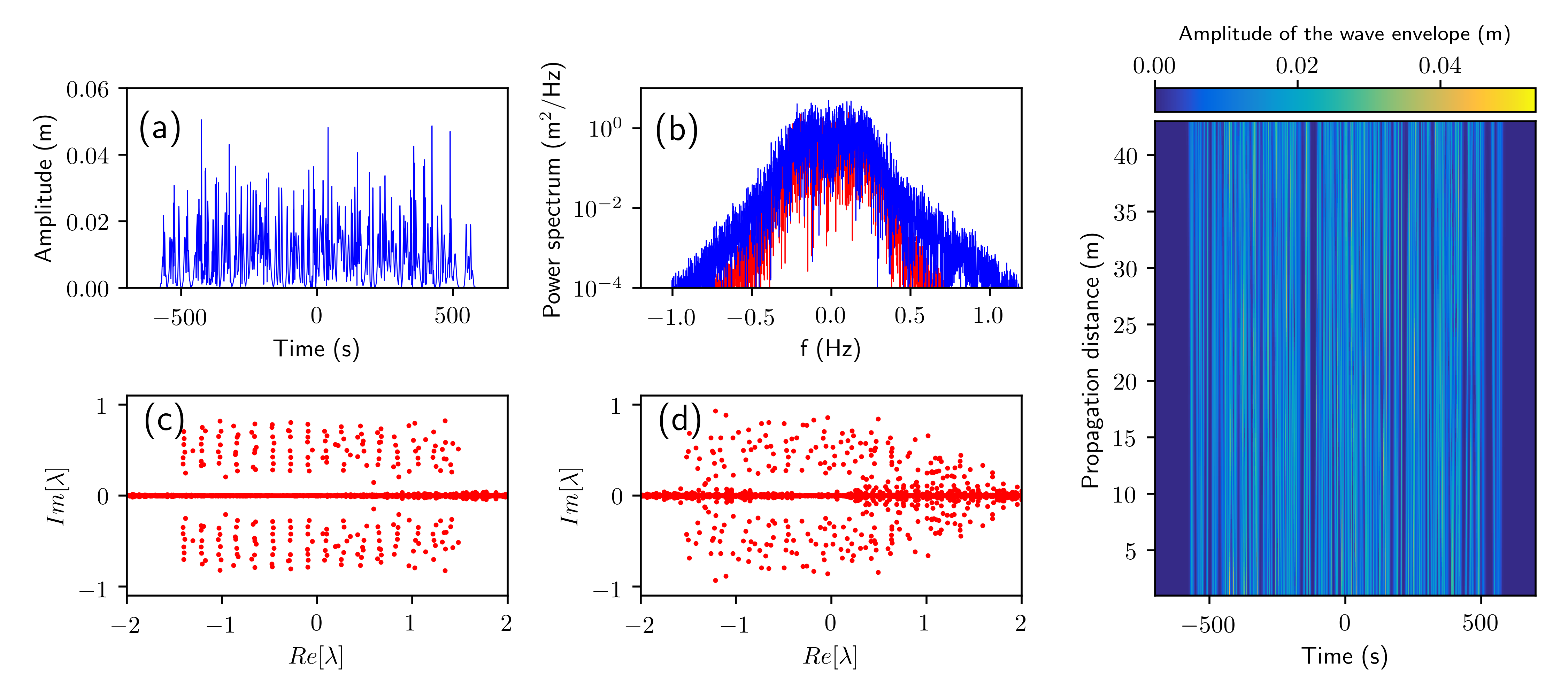
Figure S6: Numerical simlations of Eq. (S10). Gas of $N=128$ solitons propagating in the 1D water tank. (a) Modulus of the wave envelope at $Z_{1}=6$ m. (b) Fourier power spectra of wave elevation at $Z_{1}=6$ m (red line) and at $Z_{20}=120$ m (blue line). (c) Discrete IST spectrum measured at $Z_{1}=6$ m. (d) Discrete IST spectrum measured at $Z_{20}=120$ m. (e) Space-time evolution of modulus of the wave envelope. Parameters of the simulation are $f_{0}=1.15$ Hz, $k_{0}=5.32$ m^-1, $L_{NL}=45$ m ($<|A_{0}(T)|^{2}>=1.58\,\times 10^{-4}$ m².

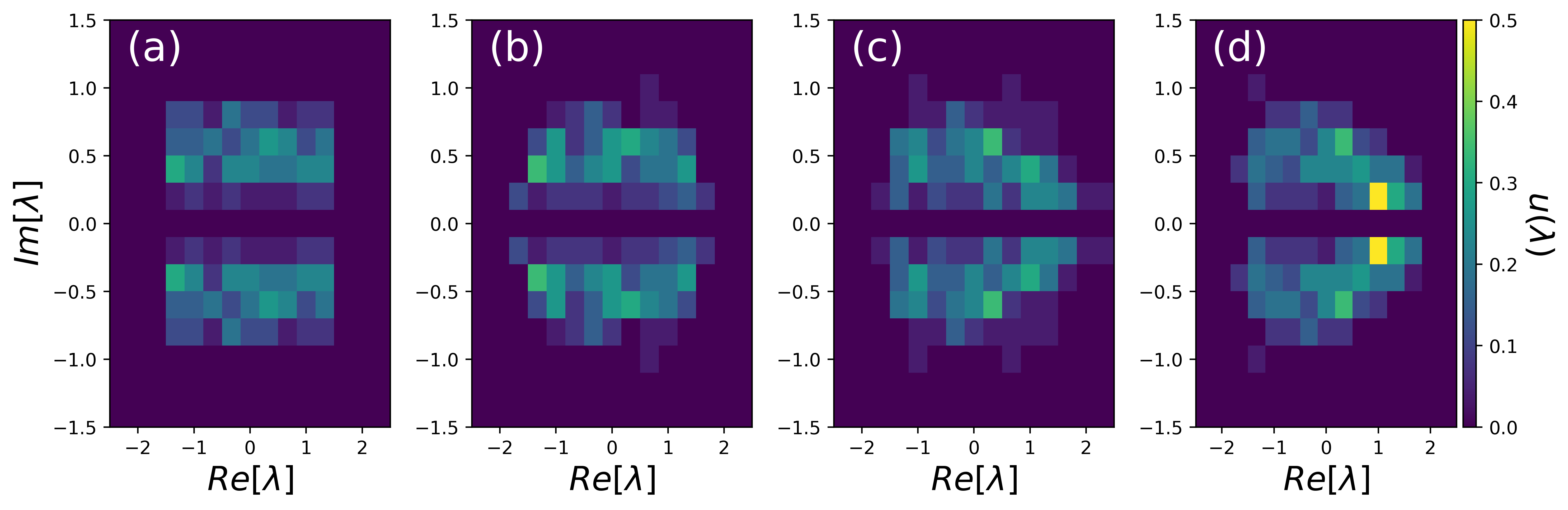
Figure S7: Numerical simlations of Eq. (S10). Statistical analysis of discrete IST spectra of Fig. S3 showing the slow evolution of the DOS $u(\lambda)$ (the probability density function of the discrete IST eigenvalues in the complex plane) as a function of propagation distance in the water tank: (a) $Z_{1}=6$ m, (b) $Z_{3}=18$ m, (c) $Z_{10}=60$ m, (d) $Z_{20}=120$ m. Parameters of the simulation are $f_{0}=1.15$ Hz, $k_{0}=5.32$ m^-1, $L_{NL}=45$ m ($<|A_{0}(T)|^{2}>=1.58\,\times 10^{-4}$ m².

V Direct numerical simulations of Euler’s equations for the gas of $128$ solitons

Direct numerical simulations of the Euler’s equations have been performed with the efficient and accurate High-Order Spectral (HOS) method Dommermuth and Yue (1987); West et al. (1987). The numerical model used in our numerical simulations reproduce the main features of the water tank, namely: i) the generation of waves through a wave maker and ii) the absorption of reflected waves with an absorbing beach. To this end a Numerical Wave Tank, entitled HOS-NWT, has been developed Ducrozet et al. (2012) (the code being available open-source COD ). It uses the exact same wave maker’s motions than in the experiments for a simplified comparison procedure. This specific model has been widely validated in different configurations and more details can be found in Ducrozet et al. (2012); Bonnefoy et al. (2010).

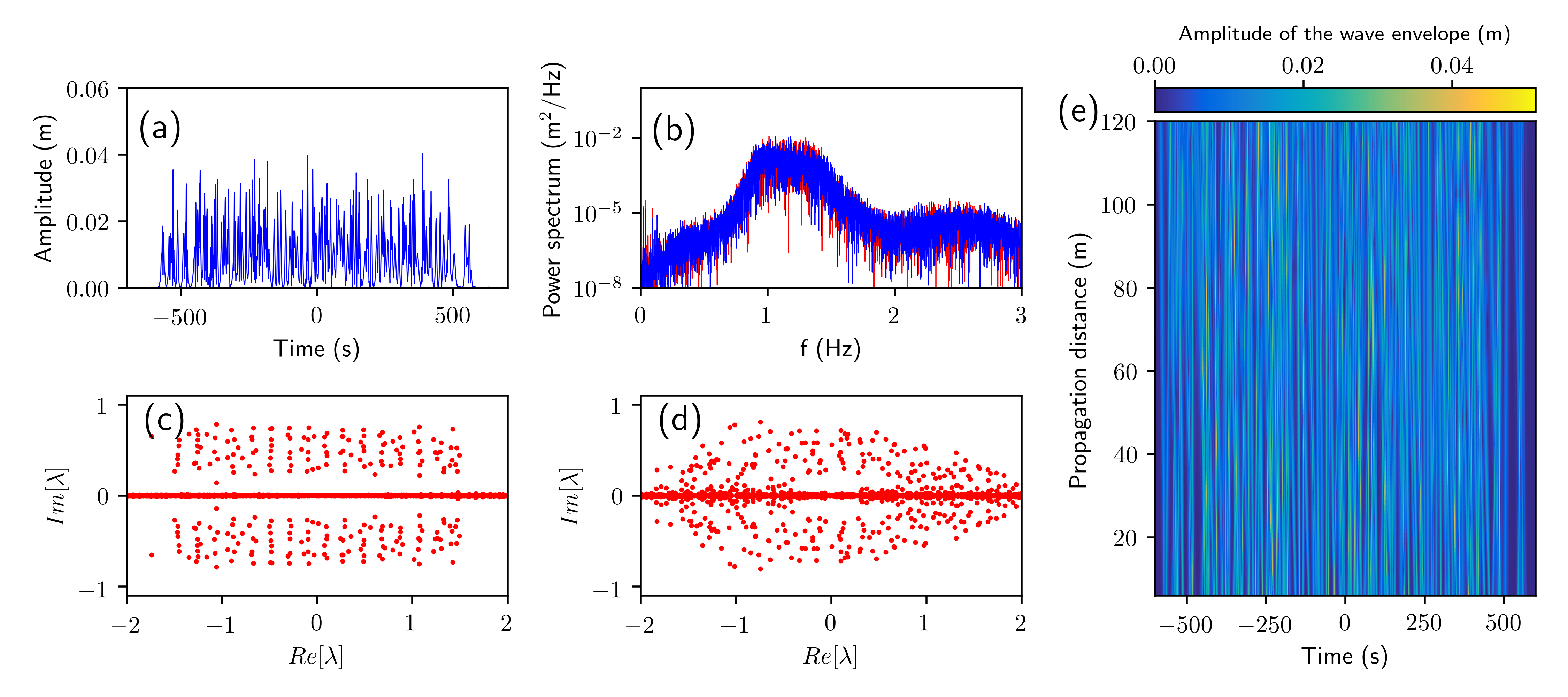
Figure S8: Numerical simulations of the Euler’s equations corresponding to the experimental results shown in Fig. 2 of the manuscript ($N=128$). (a) Modulus of the wave envelope at $Z_{1}=6$ m, close to the wavemaker. (b) Fourier power spectra of wave elevation at $Z_{1}=6$ m (blue line) and at $Z_{20}=120$ m (red line). (c) Discrete IST spectrum measured at $Z_{1}=6$ m. (d) Discrete IST spectrum measured at $Z_{20}=120$ m. (e) Space-time evolution of modulus of the wave envelope. Parameters of the simulation are $f_{0}=1.15$ Hz, $k_{0}=5.32$ m^-1, $L_{NL}=45$ m ($<|A_{0}(T)|^{2}>=1.58\,\times 10^{-4}$ m².

Fig. S5 shows numerical simulations of Euler’s equations that are made with physical values characterizing the experiments presented in the Letter for the gas of $128$ solitons. Dynamical and spectral features very similar to those reported in Fig. 2 of the Letter are found in numerical simulations reported in Fig. S4.

Fig. S6 shows the normalized density of states, i.e. the probability density function of the complex-valued discrete eigenvalues characterizing the SG. It is determined at different propagation distances from numerical simulations of Euler’s equations Dommermuth and Yue (1987); West et al. (1987).

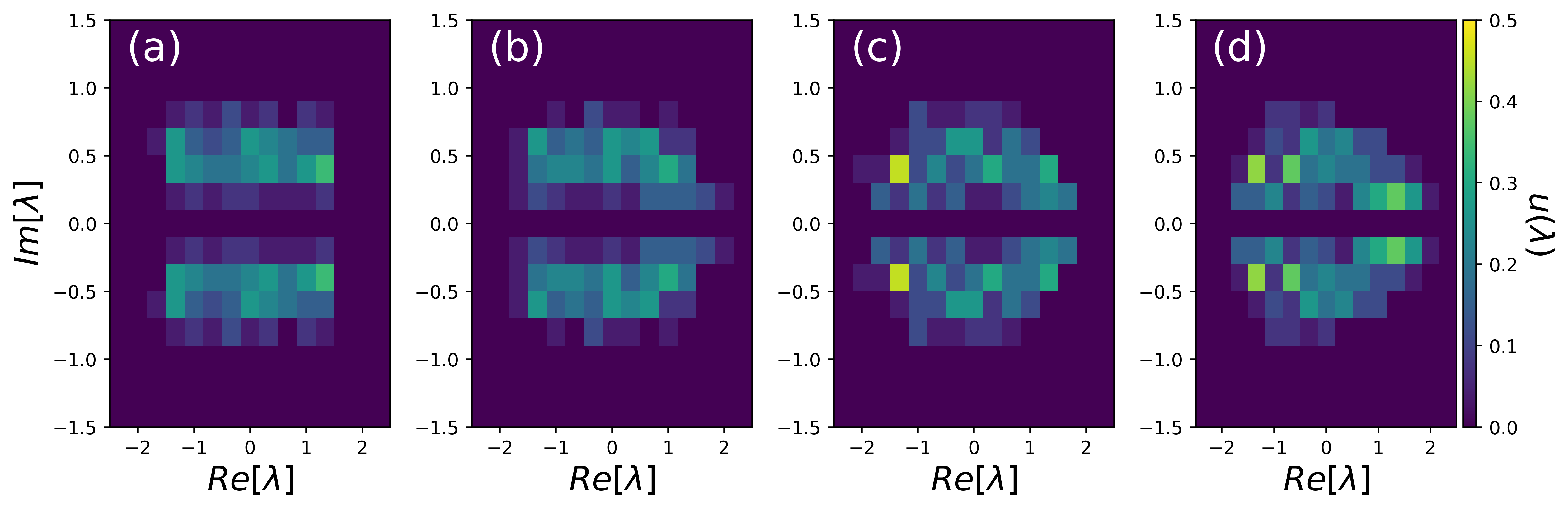
Figure S9: Numerical simlations of Eq. (S10). Statistical analysis of discrete IST spectra of Fig. S5 showing the slow evolution of the DOS $u(\lambda)$ (the probability density function of the discrete IST eigenvalues in the complex plane) as a function of propagation distance in the water tank: (a) $Z_{1}=6$ m, (b) $Z_{3}=18$ m, (c) $Z_{10}=60$ m, (d) $Z_{20}=120$ m. Parameters of the simulation are $f_{0}=1.15$ Hz, $k_{0}=5.32$ m^-1, $L_{NL}=45$ m ($<|A_{0}(T)|^{2}>=1.58\,\times 10^{-4}$ m².