Optimal Rates of Distributed Regression with Imperfect Kernels

Hongwei Sun
Department of Mathematics
University of Jinan
Jinan, Shandong, China
Email: ss_sunhw@ujn.edu.cn


Qiang Wu
Department of Mathematical Sciences
Middle Tennessee State University
Murfreesboro, TN 37132, USA
Email: qwu@mtsu.edu
Abstract

Distributed machine learning systems have been receiving increasing attentions for their efficiency to process large scale data. Many distributed frameworks have been proposed for different machine learning tasks. In this paper, we study the distributed kernel regression via the divide and conquer approach. The learning process consists of three stages. Firstly, the data is partitioned into multiple subsets. Then a base kernel regression algorithm is applied to each subset to learn a local regression model. Finally the local models are averaged to generate the final regression model for the purpose of predictive analytics or statistical inference. This approach has been proved asymptotically minimax optimal if the kernel is perfectly selected so that the true regression function lies in the associated reproducing kernel Hilbert space. However, this is usually, if not always, impractical because kernels that can only be selected via prior knowledge or a tuning process are hardly perfect. Instead it is more common that the kernel is good enough but imperfect in the sense that the true regression can be well approximated by but does not lie exactly in the kernel space. We show distributed kernel regression can still achieves capacity independent optimal rate in this case. To this end, we first establish a general framework that allows to analyze distributed regression with response weighted base algorithms by bounding the error of such algorithms on a single data set, provided that the error bounds has factored the impact of the unexplained variance of the response variable. Then we perform a leave one out analysis of the kernel ridge regression and bias corrected kernel ridge regression, which in combination with the aforementioned framework allows us to derive sharp error bounds and capacity independent optimal rates for the associated distributed kernel regression algorithms. As a byproduct of the thorough analysis, we also prove the kernel ridge regression can achieve rates faster than $O(N^{-1})$ (where $N$ is the sample size) in the noise free setting which, to our best knowledge, are first observed and novel in regression learning.

1 Introduction

Distributed machine learning systems have been receiving increasing attentions for their efficiency to process large scale data. Many distributed frameworks have been proposed for different machine learning tasks; see for instance [8, 9, 14, 5, 26, 28]. Among others, the divide and conquer approach has been proved easy to implement but efficient for statistical estimation and predictive analytics. This approach is used when the data is too big to be analyzed by one computer node and usually consists of three stages. First, the data is randomly partitioned into multiple subsets. In some applications the data may be naturally stored in different locations as a result of data collection process and there is no need for further partitioning. Second, a base algorithm is selected according to the learning task and applied to each subset to learn a local model. Finally, all local models are averaged to generate the final model. This approach is computationally efficient because the second stage can be easily parallelized. Also, because the local model training does not require mutual communication between the computing nodes, it can largely preserve privacy and confidentiality.

In the context of nonlinear regression analysis distributed kernel methods implemented via the divide and conquer approach has been widely studied and showed asymptotically minimax optimal in many situations. In particular, if the kernel is perfectly selected so that the true regression function lies in the associated reproducing kernel space, the minimax optimality was verified for kernel ridge regression [28, 23, 15], kernel spectral algorithm [11], kernel based gradient descent [16], bias corrected regularization kernel network [12], and minimum error entropy [13]. However, it is usually, if not always, impractical to select perfect kernels for real world problems. More commonly one has to select an imperfect kernel by some prior knowledge and/or a tuning process. Such a kernel is empirically optimal within a family of candidate kernels, usually good enough for applications, but there is no guarantee of perfectness. A typical example is the widely used Gaussian radial basis kernel. It is effective in most nonlinear data analysis problems because of its universality. But it is well known that its associated reproducing kernel Hilbert space consists of only infinitely differentiable functions. Functions that are not infinitely differentiable can be well approximated by the kernel but cannot lie exactly in the associated kernel space. In this situation the learning rates obtained in the literature are suboptimal.

The primary goal of this study is to verify the capacity independent optimality of distributed kernel regression algorithms when the kernel is imperfect. We focus on the use of kernel ridge regression (KRR) and bias corrected kernel ridge regression (BCKRR) in the divide and conquer approach. For this purpose, we propose a framework to analyze a broad class of distributed regression methods and conduct rigorous leave one out analyses. More specifically, we make the following four contributions.

  • First, we introduce the concept of response weighted regression algorithm, which covers a broad class of regression algorithms and has both KRR and BCKRR as examples. We propose a general framework to analyze the learning performance of response weighted distributed regression algorithms and showed that, for such algorithms, it suffices to study the learning performance of the response weighted algorithm on a single data set provided that it characterizes the impact of the unexplained variance of the response variable on the learning performance. This makes the analysis of such distributed learning algorithms much easier. Because both KRR and BCKRR fall into this framework, we will utilize it to analyze the distributed KRR and distributed BCKRR in this study.

  • Second, we conduct a leave one out analysis of the KRR algorithm and prove capacity independent error bounds, which are sharp in the sense that they lead to optimal capacity independent rates regardless the kernel is perfect or imperfect. While the idea of leave one out analysis was originally developed in [4, 27], our analysis is more rigorous so that the error bounds factor in the impact of the unexplained variance of the response variable and therefore we are able to utilize them in combination with the aforementioned framework to derive sharp error bounds and optimal learning rates for distributed KRR. Furthermore, our analysis also greatly relaxes the restriction on the number of local machines used in the distributed regression. In particular, our results indicate that fast rates can still be achieved with the number of local machines increasing at the order of $O(\sqrt{N})$ (with $N$ being the sample size) if the true regression does lie in the kernel space. This is a significant relaxation compared with those in the literature; see detailed comparison in Section 2.3.

  • Third, we conduct a rigorous leave one out analysis of the BCKRR and utilize the results to derive error bounds and learning rates for distributed BCKRR algorithm. Again, the results are optimal from a capacity independent viewpoint when the kernel is imperfect. As the BCKRR was proposed by the idea of bias correction, its original formula involves a two-step procedure and admits an operator representation which, if not impossible, is unsuitable for leave one analysis in a natural way. To overcome this difficulty we prove two alternative formulae for the algorithm, among which the recentering regularization formula defines the target function by a Tikhonov regularization scheme and allows us to conduct leave one analysis naturally. Moreover, these two perspectives also shed light on the design of other bias corrected algorithms whose solutions do not have an explicit representation like KRR. See Section 6.1 and the discussions in Section 7 for details.

  • Last, as a byproduct of our leave one out analysis, we derive super fast learning rates for both KRR and BCKRR when the unexplained variance of the response variable becomes zero, that is, the response value is determined and noise free for any fixed input. If the kernel is perfect, the rate can be faster than $O(N^{-1})$ and even as fast as $O(N^{-2})$ in the best situation. To our best knowledge, such super fast rates for kernel regression are first observed and novel in learning theory research.

The rest of the paper is organized as follows. In Section 2 we describe the problem setting, algorithms, and the main results. Discussions and detailed comparisons between our results and those in the literature will be given. Empirical studies will be used to illustrate the effectiveness of imperfect kernels in distributed regression. In Section 3 we propose a general framework for the analysis of response weighted distributed regression algorithms. Some preliminary lemmas were proved in Section 4. Then in Section 5 and Section 6 we conduct leave one out analyses of KRR and BCKRR, respectively. The results are then used to prove our main results regarding the error bounds and learning rates of distributed KRR and distributed BCKRR. We close with conclusions and discussions in Section 7.

2 Problem setting and main results

Let $\mathcal{X}$ be the sample space of input variable $x$ and $\mathcal{Y}$ the sample space of the response variable $y.$ They are linked by joint a probability measure $\rho$ on the product space $\mathcal{X}\times\mathcal{Y}.$ The goal is to learn the mean regression function that minimizes the mean squared prediction error, i.e.,

$$f^{*}=\arg\min\mathcal{E}(f)\qquad\hbox{ where }\mathcal{E}(f)=\mathbf{E}[(y-f(x))^{2}].$$

This is usually implemented by minimizing the empirical mean squared error or its regularized version when we have in hand a sampled data set $D=\{(x_{i},y_{i}),i=1,\ldots,N\}$. If $f^{*}$ is linear, multiple linear regression or the regularized methods such as ridge regression or LASSO performs well. When $f^{*}$ is nonlinear, kernel ridge regression can be used to search a good approximating function in a suitable reproducing kernel Hilbert space.

Let $K$ be a Mercer kernel, namely, a continuous, symmetric, and positive-semidefinite function $K:\mathcal{X}\times\cal X\to\mathbb{R}$. The inner product defined by $\langle K(x,\cdot),K(t,\cdot)\rangle_{K}=K(x,t)$ induces a reproducing kernel Hilbert space (RKHS) $\mathcal{H}_{K}$ associated to the kernel $K$. The space is the closure of the function class spanned by $\{K_{x}=K(x,\cdot):x\in\mathcal{X}\}.$ The reproducing property $f(x)=\langle f,K_{x}\rangle_{K}$ leads to $|f(x)|\leq\sqrt{K(x,x)}\|f\|_{K}$. Thus if $\kappa=\sup_{x\in\mathcal{X}}\sqrt{K(x,x)}<\infty$, then $\mathcal{H}_{K}$ can be embedded into $C(\mathcal{X})$ and $\|f\|_{\infty}\leq\kappa\|f\|_{K}.$ We refer to [1] for more other properties of RKHS. The kernel ridge regression (KRR) estimates the true regression function $f^{*}$ by the function $f_{D,\lambda}\in\mathcal{H}_{K}$ minimizing the regularized sample mean squared error,

$$f_{D,\lambda}=\arg\min_{f\in\mathcal{H}_{K}}\left\{\frac{1}{N}\sum_{i=1}^{N}(y_{i}-f(x_{i}))^{2}+\lambda\|f\|_{K}^{2}\right\},$$ (1)

where $\lambda>0$ is a regularization parameter. It is a popular kernel method for nonlinear regression analysis. Its predictive consistency has been extensively studied in the literature; see e.g. [10, 4, 27, 7, 25, 2, 6, 19, 22, 20] and many references therein. Its applications were also extensively explored and shown successful in many problem domains.

By the famous representer theorem, $f_{D,\lambda}$ admits a representation $f_{D,\lambda}(x)=\sum_{i=1}^{N}c_{i}K(x_{i},x)$ with $\mathbf{c}=(c_{1},\ldots,c_{N})^{\top}\in\mathbb{R}^{N}$ solved from the linear system $(\lambda N\mathbb{I}+\mathbb{K})\mathbf{c}=\mathbf{y}$ where $\mathbb{I}$ is the identity matrix, $\mathbb{K}=[K(x_{i},x_{j})]_{i,j=1}^{N}$ is the kernel matrix on the input data and $\mathbf{y}=(y_{1},\ldots,y_{N})^{\top}\in\mathbb{R}^{N}.$ Let $S:\mathcal{H}_{K}\to\mathbb{R}^{N}$ be be the sampling operator defined by $Sf=(f(x_{1}),\ldots,f(x_{N}))^{\top}$ for $f\in\mathcal{H}_{K}.$ Its dual operator $S^{*}$ is given by $S^{*}\mathbf{c}=\sum_{i=1}^{N}c_{i}K(x_{i},\cdot)\in\mathcal{H}_{K}$ for $\mathbf{c}\in\mathbb{R}^{N}.$ In [19] it is proved that $f_{D,\lambda}$ has an operator representation

$$f_{D,\lambda}=\frac{1}{N}\left(\lambda I+\frac{1}{N}S^{*}S\right)^{-1}S^{*}\mathbf{y}.$$ (2)

One objective of this paper is to study the performance of the distributed version of this method.

We need several assumptions that are used throughout the paper. Recall the true regression function is $f^{*}(x)=\mathbf{E}[y|x]$ and define $\sigma^{2}=\mathbf{E}[{\rm var}(y|x)]=\mathbf{E}[(y-f^{*}(x))^{2}].$ Notice that

$${\rm var}(y)=\mathbf{E}\Big{[}{\rm var}(y|x)\Big{]}+{\rm var}\Big{(}\mathbf{E}[y|x]\Big{)}=\sigma^{2}+{\rm var}\Big{(}f^{*}(x)\Big{)}.$$

The second term on the right is the part of variance of $y$ that is explained by the regression function while the first term is unexplained. Our first assumption is on the finiteness of unexplained variance.

Assumption 1. The unexplained variance of the response variable is finite, i.e., $\sigma^{2}<\infty.$

If in particular $\sigma^{2}=0,$ then $y=f^{*}(x)$ is determined for each given $x\in\mathcal{X}$ and we call the regression problem is noise free. Note also for any function $f$ independent of $(x,y)$ there holds

$$\mathbf{E}\left[(y-f(x))^{2}\right]=\mathbf{E}\left[(f^{\ast}(x)-f(x))^{2}\right]+\sigma^{2}.$$ (3)

This identity will be repeatedly used in the proof of our main results.

Next we need the so called source condition. To state it, let $\rho_{\!{}_{\mathcal{X}}}$ denote the marginal distribution on $\mathcal{X}.$ Define

$$L_{K}f(x)=\int_{\mathcal{X}}K(x,t)f(t)\hbox{d}\rho_{\!{}_{\mathcal{X}}}(t).$$

Then $L_{K}$ defines a compact operator both on ${L^{2}_{\rho_{\!{}_{\mathcal{X}}}}}$ (the space of square integrable functions with respect to the probability measure $\rho_{\!{}_{\mathcal{X}}}$) and $\mathcal{H}_{K}.$ Let $\tau_{i}$ and $\phi_{i}$ be the eigenvalues and eigenfunctions of $L_{K}$ as an operator on ${L^{2}_{\rho_{\!{}_{\mathcal{X}}}}}$. Then $\{\phi_{i}\}_{i=1}^{\infty}$ form an orthogonal basis of ${L^{2}_{\rho_{\!{}_{\mathcal{X}}}}}$ and

$$L_{K}f=\sum_{i=1}^{\infty}\tau_{i}\langle f,\phi_{i}\rangle_{\!{}_{{L^{2}_{\rho_{\!{}_{\mathcal{X}}}}}}}\phi_{i},\qquad\forall\ f\in{L^{2}_{\rho_{\!{}_{\mathcal{X}}}}}.$$

Also, $\{\psi_{i}=\sqrt{\tau_{i}}\phi_{i}:\tau_{i}\not=0\}$ form an orthonormal basis of $\mathcal{H}_{K}$ and, as an operator on $\mathcal{H}_{K}$,

$$L_{K}f=\sum_{i:\tau_{i}\not=0}\tau_{i}\langle f,\psi_{i}\rangle_{\!{}_{K}}\psi_{i},\qquad\forall\ f\in\mathcal{H}_{K}.$$

It is easy to verify that $L_{K}$ is a population version of the operator $\frac{1}{N}S^{*}S$ (as operators on $\mathcal{H}_{K}$).

Because $L_{K}$ is compact and admits an eigen-decomposition form, $L_{K}^{r}$ is well defined for all $r>0.$ In particular, let $\overline{\mathcal{H}_{K}}$ be the closure of $\mathcal{H}_{K}$ in ${L^{2}_{\rho_{\!{}_{\mathcal{X}}}}}.$ Then for each $f\in\overline{\mathcal{H}_{K}}$ we have $L_{K}^{\frac{1}{2}}f\in\mathcal{H}_{K}$ and

$$\|f\|_{L^{2}_{\rho_{\!{}_{\mathcal{X}}}}}=\|L^{\frac{1}{2}}f\|_{K}.$$ (4)

If the kernel $K$ is universal in the sense that $\mathcal{H}_{K}$ is dense in $C(\mathcal{X})$, then $\overline{\mathcal{H}_{K}}={L^{2}_{\rho_{\!{}_{\mathcal{X}}}}}$ and (4) holds for all $f\in{L^{2}_{\rho_{\!{}_{\mathcal{X}}}}}.$ The source condition is stated as follows.

Assumption 2. There exist some $u^{*}\in{L^{2}_{\rho_{\!{}_{\mathcal{X}}}}}$ and $r>0$ such that $f^{*}=L_{K}^{r}u^{*}.$

If the source condition holds with $r\geq\frac{1}{2}$ then $f^{*}\in\mathcal{H}_{K}$ and the kernel is perfect for learning the regression function. If $r<\frac{1}{2}$, then $f^{*}$ does not lie in $\mathcal{H}_{K}$ and the kernel is imperfect. We will focus our study on the imperfect case in this paper.

Before moving on to the distributed KRR, let us first recall that if the source condition holds with $0<r\leq 1$, KRR can reach the optimal capacity independent rate $O(N^{-\frac{2r}{1+2r}})$ [27]. If $\frac{1}{2}\leq r\leq 1$ and in addition the capacity of the reproducing kernel Hilbert space as measured by the effective dimension satisfies

$$\mathcal{N}(\lambda)=\hbox{Tr}((\lambda I+L_{K})^{-1}L_{K})\leq C_{0}\lambda^{-\beta}$$ (5)

for some $C_{0}>0$ and $0<\beta<1,$ KRR reaches the minimax optimal capacity dependent rate $O(N^{-\frac{2r}{\beta+2r}})$ [6]. However, to our best knowledge, if $r<\frac{1}{2}$ meaning that the kernel is imperfect, such minimax optimality has never been verified in the literature. Note all our results in this paper will not assume any capacity conditions.

2.1 Distributed kernel ridge regression

In the context of distributed kernel regression we divide the whole data $D$ into $m$ disjoint subset $D=\bigcup_{\ell=1}^{m}D_{\ell}.$ Without loss of generality we assume all data sets are of equal size $n=N/m$ and denote $D_{\ell}=\{(x_{\ell,1},y_{\ell,1}),\ldots,(x_{\ell,n},y_{\ell,n})\}.$ Let $f_{D_{\ell},\lambda}$ be the local estimator learned from $D_{\ell}$ by using KRR method (1). The distributed KRR defines the final global estimator by

$$\overline{f_{D,\lambda}}=\sum_{\ell=1}^{m}\frac{n}{N}f_{D_{\ell},\lambda}=\frac{1}{m}\sum_{\ell=1}^{m}f_{D_{\ell},\lambda}.$$ (6)

This approach has been studied in [28, 15] and the minimax optimality was verified for $\frac{1}{2}\leq r\leq 1$. In this paper we prove the following capacity independent bounds for all $r>0.$

Theorem 1.

Assume $\sigma^{2}<\infty$ and $f^{*}=L_{K}^{r}u^{*}$ for some $u^{*}\in L^{2}(P_{\mathcal{X}})$ and $0<r\leq 1.$

  1. (i)

    If $0<r\leq\frac{1}{2}$, then there exists a constant $C_{1}>0$ independent of $N,$ $n,$ $m$, or $\lambda$ such that

    $$\mathbf{E}\left[\left\|\overline{f_{D,\lambda}}-f^{*}\right\|^{2}_{{L^{2}_{\rho_{\!{}_{\mathcal{X}}}}}}\right]\leq C_{1}\left\{\frac{m\sigma^{2}}{N^{2}\lambda^{2}}+\frac{\sigma^{2}}{N\lambda}+\lambda^{2r}\bigg{(}1+\frac{m^{2}}{N^{2}\lambda^{2}}+\frac{m}{N\lambda}\bigg{)}\right\}.$$

    Consequently, if $m\leq N^{\frac{2r}{1+2r}},$ then with the choice $\lambda=N^{-\frac{1}{1+2r}}$, we have

    $$\mathbf{E}\left[\left\|\overline{f_{D,\lambda}}-f^{*}\right\|^{2}_{{L^{2}_{\rho_{\!{}_{\mathcal{X}}}}}}\right]=O\Big{(}N^{-\frac{2r}{1+2r}}\Big{)}.$$
  2. (ii)

    If $\frac{1}{2}<r\leq 1$ and $\lambda n\geq 1$, then there exists a constant $C_{2}>0$ such that

    $$\mathbf{E}\left[\left\|\overline{f_{D,\lambda}}-f^{*}\right\|^{2}_{{L^{2}_{\rho_{\!{}_{\mathcal{X}}}}}}\right]\leq C_{2}\left\{\frac{m\sigma^{2}}{N^{2}\lambda^{2}}+\frac{\sigma^{2}}{N\lambda}+\lambda^{2r}+\frac{\lambda^{r}m^{\frac{r}{2}+\frac{1}{4}}}{N^{\frac{r}{2}+\frac{1}{4}}}\right\}.$$

    Consequently, if $m\leq N^{\frac{4r^{2}+1}{(1+2r)^{2}}},$ then with the choice $\lambda=N^{-\frac{1}{1+2r}}$, we have

    $$\mathbf{E}\left[\left\|\overline{f_{D,\lambda}}-f^{*}\right\|^{2}_{{L^{2}_{\rho_{\!{}_{\mathcal{X}}}}}}\right]=O\Big{(}N^{-\frac{2r}{1+2r}}\Big{)}.$$

Note if $r>1$ the error bounds and convergence rates are the same as $r=1$ due to the saturation effect of KRR and have been omitted. The error bounds in Theorem 1 are sharp and the rates are capacity independent optimal. A detailed comparison with the results in the literature are given in Section 2.3.

2.2 Bias correction

The bias corrected kernel ridge regression (BCKRR) was proposed in [24] to efficiently handle block wise data, for which the distributed learning is an example. Notice the operator representation (2) implies $f_{D,\lambda}$ has asymptotic bias $-\lambda(\lambda I+L_{K})^{-1}f^{*}$. The BCKRR is formulated by subtracting an empirical estimate of the asymptotic bias:

$$f^{\sharp}_{D,\lambda}=f_{D,\lambda}+\lambda\left(\lambda I+\frac{1}{n}S^{*}S\right)^{-1}f_{D,\lambda}.$$ (7)

Similar to distributed KRR, a distributed BCKRR can be designed by applying BCKRR on each subset and averaging the local estimators to obtain the global estimator as

$$\overline{f^{\sharp}_{D,\lambda}}=\frac{1}{m}\sum_{\ell=1}^{m}f^{\sharp}_{D_{\ell},\lambda}.$$

The bias and variance of BCKRR has been characterized in [24] and the distributed BCKRR was studied in [12]. Those studies have shown that the BCKRR benefits the block wise data analysis both theoretically and empirically. Similar to the distributed KRR case, the distributed BCKRR has been shown asymptotically minimax optimal when the kernel is perfect. But when the kernel is imperfect, Guo et al [12] derived the rate of $O(N^{-\frac{r}{\beta+2r}})$ under the capacity condition (5). It implies a capacity independent rate of $O(N^{-\frac{r}{1+2r}}),$ which is far from optimal. Even with the capacity condition, if it is weak, say $\beta>\frac{1}{2}-r,$ the rate in [12] is still worse than the capacity independent rate $O(N^{-\frac{2r}{1+2r}})$. One of our main contributions is to address this question.

Theorem 2.

Assume $\sigma^{2}<\infty$ and $f^{*}=L_{K}^{r}u^{*}$ for some $u^{*}\in{L^{2}_{\rho_{\!{}_{\mathcal{X}}}}}$ with some $0<r\leq 2.$ If $\lambda n\geq 1$, then there exists a constant $\widetilde{C}>0$ independent of $N,$ $n,$ $m$, or $\lambda$ such that

$$\mathbf{E}\left[\left\|\overline{f^{\sharp}_{D,\lambda}}-f^{*}\right\|^{2}_{{L^{2}_{\rho_{\!{}_{\mathcal{X}}}}}}\right]\leq\widetilde{C}\begin{cases}\dfrac{\sigma^{2}}{N\lambda}+\lambda^{2r},&\hbox{ if }0<r\leq\frac{1}{2};\\[10.00002pt] \dfrac{\sigma^{2}}{N\lambda}+\lambda^{2r}+\dfrac{\lambda^{r}m^{\frac{r}{2}+\frac{1}{4}}}{N^{\frac{r}{2}+\frac{1}{4}}},&\hbox{ if }\frac{1}{2}<r\leq 1;\\[10.00002pt] \lambda^{2r}+\dfrac{\lambda^{r}m^{\frac{r}{2}+\frac{1}{4}}}{N^{\frac{r}{2}+\frac{1}{4}}}+\dfrac{\lambda^{r+\frac{1}{2}}m^{\frac{1}{2}}}{N^{\frac{1}{2}}}+\dfrac{\sigma^{2}}{\lambda N},&\hbox{ if }1<r\leq\frac{3}{2};\\[10.00002pt] \lambda^{2r}+\dfrac{\lambda m}{N}+\dfrac{\lambda^{r+\frac{1}{2}}m^{\frac{1}{2}}}{N^{\frac{1}{2}}}+\dfrac{\sigma^{2}}{\lambda N},&\hbox{ if }\frac{3}{2}<r\leq 2.\end{cases}$$

Consequently, if choosing $\lambda=N^{-\frac{1}{2r+1}}$ and the number of local machines satisfies $m\leq N^{\theta}$ with

$$\theta=\begin{cases}\dfrac{2r}{1+2r},&\hbox{ if }0<r\leq\frac{1}{2};\\[10.00002pt] \dfrac{4r^{2}+1}{(1+2r)^{2}},&\hbox{ if }\frac{1}{2}<r\leq\frac{1+\sqrt{2}}{2};\\[10.00002pt] \dfrac{2}{1+2r},&\hbox{ if }\frac{1+\sqrt{2}}{2}<r\leq 2,\end{cases}$$

then we have

$$\mathbf{E}\left[\left\|\overline{f^{\sharp}_{D,\lambda}}-f^{*}\right\|^{2}_{{L^{2}_{\rho_{\!{}_{\mathcal{X}}}}}}\right]=O\Big{(}N^{-\frac{2r}{1+2r}}\Big{)}.$$

2.3 Comparison with literature

The minimax rate analysis of regularized least square algorithm have been extensively studied in statistics and learning theory literature. If the eigenvalues of the operator $L_{K}$ decays as $\tau_{i}\leq i^{-\frac{1}{\beta}}$, which implies the capacity condition (5), then the minimax learning rate of kernel ridge regression is $O(N^{-\frac{2r}{2r+\beta}})$ for $\frac{1}{2}\leq r\leq 1$; see e.g. [6, 15, 3]. To our best knowledge, this rate has never been proved for $r<\frac{1}{2}$ without imposing additional conditions.

Note that the capacity condition (5) roughly measures the smoothness of kernel $K$. The smoother the kernel is, the smaller the $\beta.$ For example, it is proved in [17] that, if $K\in C^{\alpha}(\mathcal{X}^{2}\times\mathcal{X}^{2})$ with some integer $\alpha\geq 1$ and $\mathcal{X}^{2}$ is locally the graph of a Lipschitz function, then (5) is satisfied with $\beta=\left(\frac{\alpha}{2\mathrm{dim}(\mathcal{X})}+\frac{1}{2}\right)^{-1}$. Moreover, the Mercer theorem guarantees all kernels satisfies (5) with $\beta=1$. Therefore, $\beta=1$ corresponds to the worst situation and imposing a capacity condition (5) with $\beta=1$ is equivalent to no capacity condition. We see the rate $O(N^{-\frac{2r}{2r+1}})$ is minimax optimal in a capacity independent sense. It is proved in [27] that kernel ridge regression can achieve this capacity independent optimal rate when $r\leq\frac{1}{2}.$

Concerning the distributed kernel ridge regression via the divide and conquer technique, under the assumptions that $\mathbf{E}[|\phi_{i}(x)|^{2k}]\leq A^{2k}$ for some $k>2$ and constant $A<\infty$, $\lambda_{i}\leq ai^{-\frac{1}{\beta}}$, and $f^{*}\in\mathcal{H}_{K}$ (i.e. $r=\frac{1}{2}$), it is proved in [28] that the optimal learning rate of $O(N^{-\frac{1}{1+\beta}})$ can be achieved by restricting the number of local processors

$$m\leq c_{\alpha}\left(\frac{N^{\frac{k-4-k\beta}{1+\beta}}}{A^{4k}\log^{k}N}\right)^{\frac{1}{k-2}}.$$

This unfortunately does not apply to the case $\beta=1.$ Later in [15] the minimax optimal rate was verified for all $r\in[\frac{1}{2},1]$ if $m\leq N^{\min(\frac{3(2r-1)+\beta}{5(2r+\beta)},\frac{2r-1}{2r+\beta})}$ and in [11] the restriction was relaxed to $m\leq N^{\min(\frac{2}{2r+\beta},\frac{2r-1}{2r+\beta})}.$ Although their results apply to $\beta=1$, the restriction on $m$ is strict. If $r=\frac{1}{2}$, the data is essentially not able to be distributed according to their results. The error bounds in [15, 11] also apply to $r\leq\frac{1}{2}$ but only lead to suboptimal rate $O(N^{-\frac{2r}{1+\beta}})$ with the restriction $m=O(1)$. If $\beta=1$, the capacity independent rate is $O(N^{-r}).$

In this paper our primary interest is to understand the performance of distributed kernel regression when the kernel is imperfect, i.e., when $r<\frac{1}{2}$ and thus the true regression function $f^{*}$ is not in $\mathcal{H}_{k}.$ For this case, Theorem 1 (i) tells that, with the restriction $m\leq N^{\frac{2r}{1+2r}},$ the capacity independent optimal rate $O(N^{-\frac{2r}{1+2r}})$ for $r\leq\frac{1}{2}$ can be achieved. Note this rate is even faster than the existing capacity dependent rate $O(N^{-\frac{2r}{1+\beta}})$ when $r<\frac{\beta}{2}$, let alone the capacity independent rate $O(N^{-r}).$ In other words, we proved faster rates under weaker restrictions on $m.$ More importantly, unlike previous results that requires $m=O(1)$ and thus disclaims the effectiveness of distributed kernel regression algorithms in this situation, our results instead verified their feasibility.

If $f^{*}$ lies in $\mathcal{H}_{K}$, i.e. $r\geq\frac{1}{2}$, it is as expected that the rate $O(N^{-\frac{2r}{1+2r}})$ in Theorem 1 is worse than the minimax capacity dependent rate in the literature. But comparing the restrictions on the number of local machines, we see our restriction is much relaxed. In particular, when $r$ is close to $\frac{1}{2}$, the restrictions in the literature approaches to $O(1)$. But our restriction still allows about $O(\sqrt{N})$ local machines while preserving fast rates. It is a sacrifice of convergence rates for more local machines and may be useful for applications where analysis of super big data is necessary.

Concerning the distributed BCKRR, similar conclusions can be made. When $r<\frac{1}{2}$, the rate in Theorem 2 is faster and the restriction is more relaxed than the results in [12] while when $r\geq\frac{1}{2}$ the rate is worse than those in [12] but the restriction on $m$ is greatly relaxed. As noted in [24, 12] a main theoretical advantage of BCKRR is to relax the saturation effect of KRR. Comparing Theorem 2 with Theorem 1, we see the the rate of distributed BCKRR continues improving beyond $r>1$ and ceases to improve until $r=2.$ The restriction on $m$ also continue to be relaxed to $N^{\frac{\sqrt{2}}{1+\sqrt{2}}}$ until $r=\frac{1+\sqrt{2}}{2}$.

2.4 Empirical effectiveness of imperfect kernels

In this subsection we illustrate the empirical effectiveness of using imperfect kernels in distributed regression. To this end, we adopt the example used in [28, 12]. The true regression function is given by $f^{*}(x)=\min(x,1-x)$ with $x\,{\sim}\,\hbox{Uniform}[0,1]$ and the observations are generated by the additive noise model $y_{i}=f^{*}(x_{i})+\epsilon_{i}$ where $\epsilon_{i}\,{\sim}\,N(0,\sigma^{2})$ and $\sigma^{2}=\frac{1}{5}.$ We consider two kernels: the Sobolev space kernel $K_{S}(x,t)=1+\min(x,t)$ and the Guassian kernel $K_{G}(x,t)=\exp(-(x-t)^{2}/0.3).$ Recall that $f^{*}$ belongs to $\mathcal{H}_{K_{S}}$ with $\|f^{*}\|_{K_{S}}=1$. So $K_{S}$ is a perfect kernel for this problem. Notice that the reproducing kernel Hilbert space associated to a Gaussian kernel consists only infinitely differentiable functions and even polynomials may not lie in the space [18]. We conclude $f^{*}$ does not lie in $\mathcal{H}_{K_{G}}$ and $K_{G}$ is an imperfect kernel. We generate $N=4098$ sample points and use number of partitions $m\in\{2,4,8,16,32,64,128,256,512,1024\}.$ Mean squared errors between the estimated function and the true regression function is used to measure the performance.

According to [28], if the Soboleve space kernel $K_{S}$ is used, the theoretically optimal choice of the regularization parameter is $\lambda=N^{-\frac{2}{3}}$. When Guassian kernel is used, by Theorem 1 and Theorem 2, the optimal choice of $\lambda$ should depend on the index $r$ in the source condition, which, unfortunately, is unknown. By $0<r<\frac{1}{2}$ we know the optimal choice should be $N^{-\alpha}$ with $\frac{1}{2}<\alpha<1$ and $\alpha=\frac{2}{3}$ seems an acceptable choice. So we will also use $\lambda=N^{-\frac{2}{3}}$ for the Guassian kernel to make the first comparison between the four distributed kernel regression algorithms, namely, distributed KRR with Sobolev space kernel (DKRR-S), distributed BCKRR with Sobolev space kernel (DBCKRR-S), distributed KRR with Guassian kernel (DKRR-G), and distributed BCKRR with Gaussian kernel (DBCKRR-G). To do this, for each aforementioned $m$ value and each algorithm, we repeat the experiment 50 times and report the mean squared errors in Figure 1(a). The results indicate that, even if $K_{G}$ is imperfect for the problem, it performs comparable with the perfect kernel $K_{S}$ when $m$ is small and may even outperforms $K_{S}$ when $m$ becomes large.

To our best knowledge, all rate analysis literature of distributed kernel regression, including [28, 15, 16, 12, 11] and this study, suggest the optimal regularization parameter be selected as $\lambda=N^{-\alpha}$ with $\alpha$ an index depending on the regularity of the true regression function $f^{*}.$ While this is very helpful for researchers to understand the optimality of the algorithms, it is less informative for their practical use because such an index is unknown for real problems. Furthermore, distributed kernel regression becomes necessary only if the data is too big to be processed by a single machine. In this situation, it is imaginable that globally tuning the optimal parameter is either impossible or too time consuming. At the same time, note that distributed kernel regression requires underregularization, meaning that the regularization parameter must be chosen according to the total sample size $N$, not on the local sample size $n$. To resolve all these problems, [12] proposed a practical strategy to tune the parameter for distributed kernel regression. It first cross-validates the regularization parameter locally to get optimal choice $\lambda_{\ell,n}=n^{-\alpha_{\ell}}$ for each subset for $D_{\ell}$ and then use an underregularized parameter

$$\lambda_{\ell}=\lambda_{\ell,n}^{\frac{\log N}{\log n}}=N^{-\alpha_{\ell}}$$ (8)

to train the local model on $D_{\ell}.$ To mimic a real problem, now let us assume we have no information about the true regression function and the regularization parameters have to be selected by using the above tuning strategy. We run the four algorithms again for each $m$ value and report the mean squared errors in Figure 1(b). We see that, when a theoretically optimal regularization parameter is not available and $\lambda$ has to be tuned from data, the performance of all four methods deteriorates faster as $m$ increases. But Guassian kernel, though imperfect, seems less sensitive to the number of local machines and so the performance deteriorates slower than Sobolev space kernel.

Finally, the results in both plots indicate that, regardless the choices of kernels and regularization parameters, bias correction always helps to improve the learning performance and relax the restriction on the number of local machines.
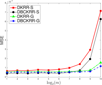
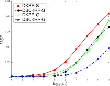
Figure 1: Mean squared error of distributed kernel regression with Sobolev space kernel and Guassian kernel when (a) the regularization parameters is fixed as $\lambda=N^{-\frac{2}{3}}$ and (b) the regularization parameter is locally tuned and underregularized according to equation (8).
Refer to caption
Refer to caption

(a) (b)

3 A framework for fast rate analysis of distributed regression

In this section we first establish a general procedure to prove fast rate for a class of regression algorithms that possess certain special features and apply to the two algorithms we study in this paper.

Definition 3.

Let $\Lambda$ be a parameter space and $\mathcal{H}$ a set of hypothesis functions. A regression algorithm $\mathcal{A}:(\mathcal{X}\times\mathcal{Y})^{N}\times\Lambda\to\mathcal{H}$ that tunes parameters in $\Lambda$ is response weighted if for any data $D\in(\mathcal{X}\times\mathcal{Y})^{N}$ and any $\lambda\in\Lambda$ there exists a vector of functions $g_{1}(D_{x},\lambda),\ldots,g_{N}(D_{x},\lambda)$ which depend only on the input data $D_{x}=\{x_{1},\ldots,x_{N}\}$ and the parameter $\lambda$ but not on the output data $D_{y}=\{y_{i}\}_{i=1}^{N}$ such that

$$\mathcal{A}(D,\lambda)=\sum_{i=1}^{N}y_{i}g_{i}(D_{x},\lambda).$$

There are many regression algorithms belonging to the response weighted family. By the representation of $f_{D,\lambda}$ and $f^{\sharp}_{D,\lambda}$, it is easy to verify that both KRR and BCKRR belong to this family. There are more examples in the literature. For instance, traditional multiple linear regression, the kernel smooth estimators, the stochastic gradient descent algorithms associated with the least square loss are all response weighted regression algorithms.

Denote by $\overline{\mathcal{A}}$ the distributed algorithm that applies the divide and conquer approach and uses $\mathcal{A}$ as the base algorithm on local subsets. It is easy to derive the following lemma.

Lemma 4.

If $\mathcal{A}$ is a response weighted regression algorithm, then $\overline{\mathcal{A}}$ is also a response weighted regression algorithm.

This lemma simply says that the response weighted feature can be inherited by the distributed algorithm. This property allows to derive fast rates for such distributed algorithms by studying error bounds of the base algorithm, as shown in the following theorem.

Theorem 5.

Let $\mathcal{A}$ be a response weighted regression algorithm and, when applying to a data $D$ of $N$ observations with parameter $\lambda,$ have the error bound as

$$\mathbf{E}\left[\|\mathcal{A}(D,\lambda)-f^{*}\|_{L^{2}_{\rho_{\!{}_{\mathcal{X}}}}}^{2}\right]\leq\varepsilon(N,\lambda,\sigma^{2}).$$

Then the corresponding distributed algorithm $\overline{\mathcal{A}}$ will have the error bound

$$\mathbf{E}\left[\|\overline{\mathcal{A}}(D,\lambda)-f^{*}\|_{L^{2}_{\rho_{\!{}_{\mathcal{X}}}}}^{2}\right]\leq\frac{\varepsilon(n,\lambda,\sigma^{2})}{m}+\varepsilon(n,\lambda,0)$$

assuming the whole data $D$ is equally split into $m$ subsets with each subset containing $n$ observations.

Proof.

Let $y^{*}_{\ell,i}=f^{*}(x_{\ell,i})$ for $1\leq\ell\leq m,$ $1\leq i\leq n$ and

$$D_{\ell}^{*}=\{(x_{\ell,1},y_{\ell,1}^{*}),\ldots,(x_{\ell,n},y_{\ell,n}^{*})\}$$

be the noise free observations associated to the subset $D_{\ell}$. We have

$$(\sigma^{*})^{2}=\mathbf{E}\Big{[}\hbox{var}\left(y_{\ell,i}^{*}|x_{\ell,i}\right)\Big{]}=\mathbf{E}\Big{[}\left(y_{\ell,i}^{*}-f^{*}(x_{\ell,i})\right)^{2}\Big{]}=0$$

and therefore

$$\mathbf{E}\left[\Big{\|}\mathcal{A}(D_{\ell}^{*},\lambda)-f^{*}\Big{\|}_{L^{2}_{\rho_{\!{}_{\mathcal{X}}}}}^{2}\right]\leq\varepsilon(n,\lambda,0).$$ (9)

Because of the response weighted feature of $\mathcal{A}$ we have

$$\mathbf{E}\Big{[}\mathcal{A}(D_{\ell},\lambda)|D_{\ell,x}\Big{]}=\sum_{i=1}^{n}\mathbf{E}[y_{\ell,i}|x_{\ell,i}]g_{i}(D_{\ell,x},\lambda)=\sum_{i=1}^{n}f^{*}(x_{\ell,i})g_{i}(D_{\ell,x},\lambda)=\mathcal{A}(D_{\ell}^{*},\lambda).$$

Therefore $\mathbf{E}\big{[}\mathcal{A}(D_{\ell},\lambda)\big{]}=\mathbf{E}\big{[}\mathcal{A}(D_{\ell}^{*},\lambda)\big{]}$ and we have

$\displaystyle\mathbf{E}\left[\|\overline{\mathcal{A}}(D,\lambda)-f^{*}\|_{L^{2}_{\rho_{\!{}_{\mathcal{X}}}}}^{2}\right]$
$\displaystyle=$ $\displaystyle\mathbf{E}\left[\left\|\frac{1}{m}\sum_{\ell=1}^{m}\Big{(}\mathcal{A}(D_{\ell},\lambda)-\mathbf{E}\left[\mathcal{A}(D_{\ell},\lambda)\right]\Big{)}\right\|_{L^{2}_{\rho_{\!{}_{\mathcal{X}}}}}^{2}\right]+\left\|\frac{1}{m}\sum_{\ell=1}^{m}\Big{(}\mathbf{E}\left[\mathcal{A}(D_{\ell},\lambda)\right]-f^{*}\Big{)}\right\|_{L^{2}_{\rho_{\!{}_{\mathcal{X}}}}}^{2}$
$\displaystyle\leq$ $\displaystyle\frac{1}{m^{2}}\sum_{\ell=1}^{m}\mathbf{E}\left[\Big{\|}\mathcal{A}(D_{\ell},\lambda)-\mathbf{E}\left[\mathcal{A}(D_{\ell},\lambda)\right]\Big{\|}_{L^{2}_{\rho_{\!{}_{\mathcal{X}}}}}^{2}\right]+\frac{1}{m}\sum_{\ell=1}^{m}\Big{\|}\ \mathbf{E}\left[\mathcal{A}(D_{\ell},\lambda)\right]-f^{*}\Big{\|}_{L^{2}_{\rho_{\!{}_{\mathcal{X}}}}}^{2}$
$\displaystyle=$ $\displaystyle\frac{1}{m^{2}}\sum_{\ell=1}^{m}\mathbf{E}\left[\Big{\|}\mathcal{A}(D_{\ell},\lambda)-f^{*}\Big{\|}_{L^{2}_{\rho_{\!{}_{\mathcal{X}}}}}^{2}\right]+\left(\frac{1}{m}-\frac{1}{m^{2}}\right)\sum_{\ell=1}^{m}\Big{\|}\mathbf{E}\left[\mathcal{A}(D_{\ell},\lambda)\right]-f^{*}\Big{\|}_{L^{2}_{\rho_{\!{}_{\mathcal{X}}}}}^{2}$
$\displaystyle\leq$ $\displaystyle\frac{1}{m^{2}}\sum_{\ell=1}^{m}\varepsilon(n,\lambda,\sigma^{2})+\frac{1}{m}\sum_{\ell=1}^{m}\mathbf{E}\left[\Big{\|}\mathcal{A}(D_{\ell}^{*},\lambda)-f^{*}\Big{\|}_{L^{2}_{\rho_{\!{}_{\mathcal{X}}}}}^{2}\right]$
$\displaystyle\leq$ $\displaystyle\frac{1}{m}\varepsilon(n,\lambda,\sigma^{2})+\varepsilon(n,\lambda,0),$

where we used (9) in the last step. ∎

Theorem 5 states that, if the base algorithm $\mathcal{A}$ admits sharper error bounds for the noise free data (i.e. $\sigma^{2}=0$), then the distributed algorithm will be able to converges fast in the sense that the distributed computing is playing a rule and produces an estimator better than the algorithm on a single subset.

In order to use this general framework to derive error bounds and fast rates for distributed algorithm, however, we must study the performance of the base algorithm on a single data with full exploration of the impact on the unexplained variance $\sigma^{2}$. Although both KRR and BCKRR have already been studied in the literature, the error bounds that clearly involve $\sigma^{2}$ and allow us to derive error bounds of their distributed version with imperfect kernels are not available. They will be our main objectives in Sections 5 and 6.

4 Preliminaries

In this section we provide some notations and preliminary lemmas that will be used in the proofs. For any regularization parameter $\lambda>0$, define

$$f_{\lambda}=\arg\min_{f\in\mathcal{H}_{K}}\left\{\|f-f^{\ast}\|^{2}_{L_{\rho_{X}}^{2}}+\lambda\|f\|_{K}^{2}\right\}.$$ (10)

It is a sample limit version of the KRR estimation $f_{D,\lambda}$ and admits an operator representation

$$f_{\lambda}=(\lambda I+L_{K})^{-1}L_{K}f^{*}.$$

It plays an essential role to characterize the approximation error of the two algorithms under study. The following lemma is well known.

Lemma 6.

Under the source condition $f^{*}=L_{K}^{r}u^{*}$ for some $r>0$ and $u^{*}\in{L^{2}_{\rho_{\!{}_{\mathcal{X}}}}}$, there hold

$$\|f_{\lambda}-f^{*}\|_{L^{2}_{\rho_{\!{}_{\mathcal{X}}}}}^{2}\leq\lambda^{\min(2r,2)}\|u^{*}\|_{L^{2}_{\rho_{\!{}_{\mathcal{X}}}}}^{2}.$$

and

$$\lambda\|f_{\lambda}\|_{K}^{2}\leq\lambda^{\min(2r,1)}\|u^{*}\|_{L^{2}_{\rho_{\!{}_{\mathcal{X}}}}}^{2}.$$

In the analysis of BCKRR, we will need the sample limit of $f_{D,\lambda}^{\sharp}$ defined by

$$f_{\lambda}^{\sharp}=f_{\lambda}+\lambda(\lambda I+L_{K})^{-1}f_{\lambda}=(\lambda I+L_{K})^{-2}(2\lambda L_{K}+L_{K}^{2})f^{*}.$$ (11)

For this function, we have the following approximation property [12].

Lemma 7.

Under the source condition $f^{*}=L_{K}^{r}u^{*}$ for some $r>0$ and $u^{*}\in{L^{2}_{\rho_{\!{}_{\mathcal{X}}}}}$, there holds

$$\|f_{\lambda}^{\sharp}-f^{*}\|_{L^{2}_{\rho_{\!{}_{\mathcal{X}}}}}^{2}\leq\lambda^{\min(2r,4)}\|u^{*}\|_{L^{2}_{\rho_{\!{}_{\mathcal{X}}}}}^{2}.$$

The following lemma can be derived from operator monotone property; see e.g. [22].

Lemma 8.

If $T_{1}$ and $T_{2}$ are two bounded self-adjoint positive operators, then for any $\alpha\in[0,1]$ there holds

$$\|T_{1}^{\alpha}-T_{2}^{\alpha}\|\leq\|T_{1}-T_{2}\|^{\alpha}.$$

The Lemma 9 below follows from simple calculation.

Lemma 9.

Let $\xi$ be a random variable with values in a Hilbert space $\mathcal{H}$ and $\{\xi_{1},\ldots,\xi_{N}\}$ be a set of i.i.d. observations for $\xi$. Then

$$\mathbf{E}\left[\left\|\frac{1}{N}\sum_{i=1}^{N}\xi_{i}-\mathbf{E}\xi\right\|^{2}\right]\leq\frac{\mathbf{E}[\|\xi\|^{2}]}{N}.$$

Let $\hbox{HS}(\mathcal{H}_{K})$ be the class of Hilbert-Schmidt operators on $\mathcal{H}_{K}$. It is known $\hbox{HS}(\mathcal{H}_{K})$ forms a Hilbert space with the Hilbert-Schmidt norm which, give an operator $A$ on $\mathcal{H}_{K},$ is defined by $\|A\|_{\hbox{\scriptsize HS}}^{2}=\hbox{Trace}(A^{*}A).$ Then $L_{K}$ as an operator on $\mathcal{H}_{K}$ belongs to $\hbox{HS}(\mathcal{H}_{K})$ and $\|L_{K}\|_{\hbox{\scriptsize HS}}\leq\kappa^{2}$; see e.g. [21]. Define the rank one operator $K_{x}\otimes K_{x}$ by

$$K_{x}\otimes K_{x}f=\langle f,K_{x}\rangle_{K}K_{x}=f(x)K_{x}.$$

Then $\|K_{x}\otimes K_{x}\|_{\hbox{\scriptsize HS}}\leq\kappa^{2}.$ Note for any all Hilbert-Schmidt operator $A$ there holds $\|A\|\leq\|A\|_{\hbox{\scriptsize HS}}$. Applying Lemma 9 to $\xi=K_{x}\otimes K_{x}$ we have the following lemma.

Lemma 10.

We have

$$\mathbf{E}\left[\left\|\frac{1}{N}S^{*}S-L_{K}\right\|^{2}\right]\leq\frac{\kappa^{4}}{N}$$

Define

$$Q(\lambda,\,N)=\min_{f\in\mathcal{H}_{K}}\left\{\|f-f^{\ast}\|_{L^{2}_{\rho_{\!{}_{\mathcal{X}}}}}^{2}+\lambda\|f\|_{K}^{2}\right\}-\lambda\mathbf{E}\left[\|f_{D,\lambda}\|_{K}^{2}\right].$$

Note that $Q(\lambda,N)$ depends on the regularization parameter $\lambda$ and sample size $N$, not on the data $D$. We will need a sharp bound for $Q(\lambda,N).$

Lemma 11.

Assume $f^{*}=L_{K}^{r}u^{*}$ for some $r>0$, $u^{*}\in{L^{2}_{\rho_{\!{}_{\mathcal{X}}}}}$.

  1. (i)

    If $0<r\leq\frac{1}{2},$ then

    $$Q(\lambda,N)\leq 2\lambda^{2r}\|u^{*}\|_{L^{2}_{\rho_{\!{}_{\mathcal{X}}}}}^{2}.$$
  2. (ii)

    If $\frac{1}{2}<r\leq 1$, then

    $$Q(\lambda,N)\leq\lambda^{2r}\|u^{*}\|_{L^{2}_{\rho_{\!{}_{\mathcal{X}}}}}^{2}\left(1+\frac{2\kappa^{2r}}{\lambda^{r}N^{\frac{r}{2}+\frac{1}{4}}}+\frac{2\kappa}{\sqrt{\lambda N}}\right).$$
  3. (iii)

    If $1<r\leq\frac{3}{2}$, then

    $$Q(\lambda,N)\leq\lambda^{2}\|u^{*}\|_{L^{2}_{\rho_{\!{}_{\mathcal{X}}}}}^{2}\left(1+\frac{2\kappa^{2r}}{\lambda N^{\frac{r}{2}+\frac{1}{4}}}+\frac{2\kappa\lambda^{r-1}}{\sqrt{\lambda N}}\right).$$
  4. (iv)

    If $r>\frac{3}{2}$, then

    $$Q(\lambda,N)\leq\lambda^{2}\|u^{*}\|_{L^{2}_{\rho_{\!{}_{\mathcal{X}}}}}^{2}\left(1+\frac{2\kappa^{3}}{\lambda N}+\frac{2\kappa}{\sqrt{N}}\right).$$
Proof.

By the definition (10) we see

$$Q(\lambda,N)=\|f_{\lambda}-f^{*}\|_{L^{2}_{\rho_{\!{}_{\mathcal{X}}}}}^{2}+\lambda\|f_{\lambda}\|_{K}^{2}-\lambda\mathbf{E}\left[\|f_{D,\lambda}\|_{K}^{2}\right].$$ (12)

We see conclusion (i) follows easily from Lemma 6.

To prove conclusions (ii)-(iv), the key is to bound $\|f_{\lambda}\|_{K}^{2}-\mathbf{E}\left[\|f_{D,\lambda}\|_{K}^{2}\right].$ To this end, first note that

$\displaystyle\|f_{\lambda}\|_{K}^{2}-\mathbf{E}\left[\|f_{D,\lambda}\|_{K}^{2}\right]$ $\displaystyle=\mathbf{E}\left[\left\langle f_{\lambda}-f_{D,\lambda},\ f_{\lambda}+f_{D,\lambda}\right\rangle_{K}\right]$
$\displaystyle=2\mathbf{E}\left[\left\langle f_{\lambda}-f_{D,\lambda},\ f_{\lambda}\right\rangle_{K}-\|f_{\lambda}-f_{D,\lambda}\|_{K}^{2}\right]$
$\displaystyle\leq 2\mathbf{E}\left[\left\langle f_{\lambda}-f_{D,\lambda},\ f_{\lambda}\right\rangle_{K}\right]$
$\displaystyle=2\left\langle f_{\lambda}-\mathbf{E}[f_{D,\lambda}],\ f_{\lambda}\right\rangle_{K}.$

By the operator representation (2) of $f_{D,\lambda}$ we have

$$\mathbf{E}[f_{D,\lambda}]=\mathbf{E}\left[\frac{1}{N}\left(\lambda I+\frac{1}{N}S^{*}S\right)^{-1}S^{*}Sf^{*}\right].$$

It is easy to verify that $f_{\lambda}-\mathbf{E}[f_{D,\lambda}]=\left(\lambda I+\frac{1}{N}S^{\ast}S\right)^{-1}U$ with $U=\big{(}\frac{1}{N}S^{*}S-L_{K}\big{)}(f_{\lambda}-f^{*}).$ Applying Lemma 9 to the $\mathcal{H}_{K}$-valued random variable $\xi=(f_{\lambda}(x)-f^{*}(x))K_{x}$ and by Lemma 6 we have

$$\mathbf{E}\left[\left\|U\right\|_{K}^{2}\right]\leq\kappa^{2}\|f_{\lambda}-f^{*}\|_{L^{2}_{\rho_{\!{}_{\mathcal{X}}}}}^{2}N^{-1}\leq{\kappa^{2}\|u^{*}\|_{L^{2}_{\rho_{\!{}_{\mathcal{X}}}}}^{2}\lambda^{\min(2r,2)}}{N^{-1}}.$$

Then, by the assumption $f^{*}=L_{K}^{r}u^{*}$ for $\frac{1}{2}<r\leq\frac{3}{2}$ and using Lemma 8, Hölder’s inequality, and Lemma 10, we obtain

$\displaystyle\left\langle f_{\lambda}-\mathbf{E}[f_{D,\lambda}],\ f_{\lambda}\right\rangle_{K}$ $\displaystyle=\mathbf{E}\left[\left\langle\Big{(}\lambda I+\frac{1}{N}S^{\ast}S\Big{)}^{-1}U,\ \Big{(}\lambda I+L_{K}\Big{)}^{-1}L_{K}^{1+r}u^{*}\right\rangle_{K}\right]$
$\displaystyle=\mathbf{E}\left[\left\langle L_{K}^{r+\frac{1}{2}}(\lambda I+L_{K})^{-1}\Big{(}\lambda I+\frac{1}{N}S^{\ast}S\Big{)}^{-1}U,\,L_{K}^{\frac{1}{2}}u^{*}\right\rangle_{K}\right]$
$\displaystyle\leq\|u^{*}\|_{L^{2}_{\rho_{\!{}_{\mathcal{X}}}}}\mathbf{E}\left[\left\|L_{K}^{r-\frac{1}{2}}\bigg{(}\lambda I+\frac{1}{N}S^{\ast}S\Big{)}^{-1}U\right\|_{K}\right]$ (13)
$\displaystyle\leq\|u^{*}\|_{L^{2}_{\rho_{\!{}_{\mathcal{X}}}}}\mathbf{E}\left[\Big{(}\lambda^{-1}\left\|L_{K}^{r-\frac{1}{2}}-\Big{(}\frac{1}{N}S^{*}S\Big{)}^{r-\frac{1}{2}}\right\|+\lambda^{r-\frac{3}{2}}\bigg{)}\|U\|_{K}\right]$
$\displaystyle\leq\|u^{*}\|_{L^{2}_{\rho_{\!{}_{\mathcal{X}}}}}\mathbf{E}\left[\Big{(}\lambda^{-1}\left\|L_{K}-\frac{1}{N}S^{*}S\right\|^{r-\frac{1}{2}}+\lambda^{r-\frac{3}{2}}\bigg{)}\|U\|_{K}\right]$
$\displaystyle\leq\|u^{*}\|_{L^{2}_{\rho_{\!{}_{\mathcal{X}}}}}\left\{\lambda^{-1}\left(\mathbf{E}\left[\left\|L_{K}-\text{\scalebox{0.8}{$\frac{1}{N}$}}S^{*}S\right\|^{2}\right]\right)^{\frac{r}{2}-\frac{1}{4}}+\lambda^{r-\frac{3}{2}}\right\}\Big{(}\mathbf{E}\left[\|U\|_{K}^{2}\right]\Big{)}^{\frac{1}{2}}$
$\displaystyle\leq\|u^{*}\|_{L^{2}_{\rho_{\!{}_{\mathcal{X}}}}}^{2}\left(\frac{\kappa^{2r}\lambda^{\min(r-1,0)}}{N^{\frac{r}{2}+\frac{1}{4}}}+\frac{\kappa\lambda^{\min(2r-\frac{3}{2},r-\frac{1}{2})}}{N^{\frac{1}{2}}}\right).$

Plugging this estimate into (12) and applying Lemma 6 again we obtain the desired bounds in conclusion (ii) and conclusion (iii).

If $r>\frac{3}{2},$ then by (13), we have

$\displaystyle\left\langle f_{\lambda}-\mathbf{E}[f_{D,\lambda}],\ f_{\lambda}\right\rangle_{K}$ $\displaystyle\leq\|u^{*}\|_{L^{2}_{\rho_{\!{}_{\mathcal{X}}}}}\mathbf{E}\left[\Big{(}\lambda^{-1}\left\|L_{K}-\frac{1}{N}S^{*}S\right\|+1\bigg{)}\|U\|_{K}\right]$
$\displaystyle\leq\|u^{*}\|_{L^{2}_{\rho_{\!{}_{\mathcal{X}}}}}^{2}\left(\frac{\kappa^{3}}{N}+\frac{\kappa\lambda}{N^{\frac{1}{2}}}\right).$

The conclusion (iv) follows by plugging this estimate into (12). ∎

Next we define

$$Q^{\sharp}(\lambda,N)=\|f_{\lambda}^{\sharp}-f^{*}\|_{L^{2}_{\rho_{\!{}_{\mathcal{X}}}}}^{2}+\lambda\left(\mathbf{E}\left[\|f_{\lambda}^{\sharp}-f_{D,\lambda}\|_{K}^{2}\right]-\mathbf{E}\left[\|f_{D,\lambda}^{\sharp}-f_{D,\lambda}\|_{K}^{2}\right]\right).$$

It will be used to derive the error bound for BCKRR when $r\geq 1.$

Lemma 12.

Assume $f^{*}=L_{K}^{r}u^{*}$ for some $\frac{1}{2}\leq r\leq\frac{3}{2}$ and $u^{*}\in{L^{2}_{\rho_{\!{}_{\mathcal{X}}}}}$. If $\lambda\leq 1$, then

$$Q^{\sharp}(\lambda,N)\leq 20(\kappa^{3}+\kappa)\|u^{*}\|_{L^{2}_{\rho_{\!{}_{\mathcal{X}}}}}^{2}\left(\lambda^{\min(2r,4)}+\frac{\lambda^{\min(2r-1,1)}}{N}+\frac{\lambda^{\min(r,1)}}{N^{\min(\frac{r}{2}+\frac{1}{4},1)}}+\frac{\lambda^{\min(2r-\frac{1}{2},r+\frac{1}{2},2)}}{N^{\frac{1}{2}}}\right)+\frac{4\kappa^{2}\sigma^{2}}{\lambda N}.$$
Proof.

First note that

$$\mathbf{E}\left[\|f_{\lambda}^{\sharp}-f_{D,\lambda}\|_{K}^{2}\right]-\mathbf{E}\left[\|f_{D,\lambda}^{\sharp}-f_{D,\lambda}\|_{K}^{2}\right]\leq 2\mathbf{E}\left[\left\langle f_{\lambda}^{\sharp}-f_{D,\lambda}^{\sharp},\ \ f_{\lambda}^{\sharp}-f_{D,\lambda}\right\rangle_{K}\right].$$

Let

$$f_{\mathbf{x},\lambda}^{\sharp}=\mathbf{E}\left[f_{D,\lambda}^{\sharp}|D_{x}\right]=\Big{(}\lambda I+\frac{1}{N}S^{*}S\Big{)}^{-2}\Big{(}2\lambda I+\frac{1}{N}S^{*}S\Big{)}\frac{1}{N}S^{*}Sf^{*}$$

and

$$f_{\mathbf{x},\lambda}=\mathbf{E}\left[f_{D,\lambda}|D_{x}\right]=\Big{(}\lambda I+\frac{1}{N}S^{*}S\Big{)}^{-1}\frac{1}{N}S^{*}Sf^{*}.$$

Then we have that

$\displaystyle\mathbf{E}\left[\left\langle f_{D,\lambda}^{\sharp},\ f_{D,\lambda}\right\rangle_{K}\right]-\mathbf{E}\left[\left\langle f_{\mathbf{x},\lambda}^{\sharp},\ f_{\mathbf{x},\lambda}\right\rangle_{K}\right]$
$\displaystyle=$ $\displaystyle\mathbf{E}\left[\left\langle\Big{(}\lambda I+\frac{1}{N}S^{*}S\Big{)}^{-2}\Big{(}2\lambda I+\frac{1}{N}S^{*}S\Big{)}\frac{1}{N}S^{*}(\mathbf{y}-Sf^{*}),\ \Big{(}\lambda I+\frac{1}{N}S^{*}S\Big{)}^{-1}\frac{1}{N}S^{*}(\mathbf{y}-Sf^{*})\right\rangle_{K}\right]$
$\displaystyle=$ $\displaystyle\mathbf{E}\left[\left\|\Big{(}\lambda I+\frac{1}{N}S^{*}S\Big{)}^{-1}\frac{1}{N}S^{*}(\mathbf{y}-Sf^{*})\right\|_{K}^{2}\right]+\mathbf{E}\left[\left\|\lambda^{\frac{1}{2}}\Big{(}\lambda I+\frac{1}{N}S^{*}S\Big{)}^{-\frac{3}{2}}\frac{1}{N}S^{*}(\mathbf{y}-Sf^{*})\right\|_{K}^{2}\right]$
$\displaystyle\leq$ $\displaystyle 2\lambda^{-2}\mathbf{E}\left[\left\|\frac{1}{N}S^{*}(\mathbf{y}-Sf^{*})\right\|_{K}^{2}\right]\leq\frac{2\kappa^{2}\sigma^{2}}{\lambda^{2}N}.$

Therefore,

$$\mathbf{E}\left[\|f_{\lambda}^{\sharp}-f_{D,\lambda}\|_{K}^{2}\right]-\mathbf{E}\left[\|f_{D,\lambda}^{\sharp}-f_{D,\lambda}\|_{K}^{2}\right]\leq 2\mathbf{E}\left[\left\langle f_{\lambda}^{\sharp}-f_{x,\lambda}^{\sharp},\ \ f_{\lambda}^{\sharp}-f_{x,\lambda}\right\rangle_{K}\right]+\frac{4\kappa^{2}\sigma^{2}}{\lambda^{2}N}.$$

By the fact $\lambda^{2}f_{\lambda}^{\sharp}=(2\lambda L_{K}+L_{K}^{2})(f^{*}-f_{\lambda}^{\sharp})$ we have

$\displaystyle f_{\lambda}^{\sharp}-f_{\mathbf{x},\lambda}^{\sharp}$ $\displaystyle=\Big{(}\lambda I+\frac{1}{N}S^{*}S\Big{)}^{-2}\left\{\Big{(}2\lambda I+\frac{1}{N}S^{*}S\Big{)}\frac{1}{N}S^{*}S-(2\lambda I+L_{K})L_{K}\right\}(f_{\lambda}^{\sharp}-f^{*})$
$\displaystyle=\Big{(}\lambda I+\frac{1}{N}S^{*}S\Big{)}^{-2}\Big{(}2\lambda I+\frac{1}{N}S^{*}S\Big{)}\Big{(}\frac{1}{N}S^{*}S-L_{K}\Big{)}(f_{\lambda}^{\sharp}-f^{*})$
$\displaystyle\quad+\Big{(}\lambda I+\frac{1}{N}S^{*}S\Big{)}^{-2}\Big{(}\frac{1}{N}S^{*}S-L_{K}\Big{)}L_{K}(f_{\lambda}^{\sharp}-f^{*}).$

Applying Lemma 9 to the random variable $\xi=(f^{*}(x)-f_{\lambda}^{\sharp}(x))K_{x}$ and by Lemma 7 we obtain

$$\mathbf{E}\left[\left\|\Big{(}\frac{1}{N}S^{*}S-L_{K}\Big{)}(f_{\lambda}^{\sharp}-f^{*})\right\|_{K}^{2}\right]\leq\frac{\kappa^{2}\|f_{\lambda}^{\sharp}-f^{*}\|_{L^{2}_{\rho_{\!{}_{\mathcal{X}}}}}^{2}}{N}\leq\frac{\kappa^{2}\|u^{*}\|_{L^{2}_{\rho_{\!{}_{\mathcal{X}}}}}^{2}\lambda^{\min(2r,4)}}{N}.$$

Similarly, we have

$$\mathbf{E}\left[\left\|\Big{(}\frac{1}{N}S^{*}S-L_{K}\Big{)}L_{K}(f_{\lambda}^{\sharp}-f^{*})\right\|_{K}^{2}\right]\leq\frac{\kappa^{2}\|L_{K}(f_{\lambda}^{\sharp}-f^{*})\|_{L^{2}_{\rho_{\!{}_{\mathcal{X}}}}}^{2}}{N}\leq\frac{\kappa^{2}\|u^{*}\|_{L^{2}_{\rho_{\!{}_{\mathcal{X}}}}}^{2}\lambda^{\min(2r+2,4)}}{N}.$$

Hence we have

$\displaystyle\mathbf{E}\left[\left\|f_{\lambda}^{\sharp}-f_{\mathbf{x},\lambda}^{\sharp}\right\|_{K}^{2}\right]\leq\frac{10\kappa^{2}\|u^{*}\|_{L^{2}_{\rho_{\!{}_{\mathcal{X}}}}}^{2}\lambda^{\min(2r-2,0)}}{N}$

and

$\displaystyle\mathbf{E}\left[\left\|\Big{(}\lambda I+\frac{1}{N}S^{*}S\Big{)}\Big{(}f_{\lambda}^{\sharp}-f_{\mathbf{x},\lambda}^{\sharp}\Big{)}\right\|_{K}^{2}\right]\leq\frac{10\kappa^{2}\|u^{*}\|_{L^{2}_{\rho_{\!{}_{\mathcal{X}}}}}^{2}\lambda^{\min(2r,2)}}{N}$

By Lemma 8 and Lemma 10 we have

$\displaystyle\mathbf{E}\left[\left\|\Big{(}\lambda I+\frac{1}{N}S^{*}S\Big{)}^{-1}\Big{(}f_{\mathbf{x},\lambda}^{\sharp}-f_{\mathbf{x},\lambda}\Big{)}\right\|_{K}^{2}\right]$ $\displaystyle=\mathbf{E}\left[\left\|\lambda\Big{(}\lambda I+\frac{1}{N}S^{*}S\Big{)}^{-3}\frac{1}{N}S^{*}SL_{K}^{r}u^{*}\right\|_{K}^{2}\right]$
$\displaystyle\leq 2\|u^{*}\|_{L^{2}_{\rho_{\!{}_{\mathcal{X}}}}}^{2}\left(\lambda^{-2}\mathbf{E}\left[\left\|L_{K}^{r-\frac{1}{2}}-\Big{(}\frac{1}{N}S^{*}S\Big{)}^{r-\frac{1}{2}}\right\|^{2}\right]+\lambda^{2r-3}\right)$
$\displaystyle\leq 2\|u^{*}\|_{L^{2}_{\rho_{\!{}_{\mathcal{X}}}}}^{2}\left(\frac{\kappa^{4r-2}}{\lambda^{2}N^{\min(r-\frac{1}{2},1)}}+\lambda^{\min(2r-3,0)}\right).$

So we have

$\displaystyle\mathbf{E}\left[\left\langle f_{\lambda}^{\sharp}-f_{\mathbf{x},\lambda}^{\sharp},\ \ f_{\lambda}^{\sharp}-f_{\mathbf{x},\lambda}\right\rangle_{K}\right]\leq\mathbf{E}\left[\left\|f_{\lambda}^{\sharp}-f_{\mathbf{x},\lambda}^{\sharp}\right\|_{K}^{2}\right]+\mathbf{E}\left[\left\langle f_{\lambda}^{\sharp}-f_{\mathbf{x},\lambda}^{\sharp},\ \ f_{\mathbf{x},\lambda}^{\sharp}-f_{\mathbf{x},\lambda}\right\rangle_{K}\right]$
$\displaystyle\leq$ $\displaystyle 10(\kappa^{3}+\kappa)\|u^{*}\|_{L^{2}_{\rho_{\!{}_{\mathcal{X}}}}}^{2}\left(\frac{\lambda^{\min(2r-2,0)}}{N}+\frac{\lambda^{\min(r-1,0)}}{N^{\min(\frac{r}{2}+\frac{1}{4},1)}}+\frac{\lambda^{\min(2r-\frac{3}{2},r-\frac{1}{2},1)}}{N^{\frac{1}{2}}}\right)$

and therefore

$\displaystyle\lambda\left(\mathbf{E}\left[\|f_{\lambda}^{\sharp}-f_{D,\lambda}\|_{K}^{2}\right]-\mathbf{E}\left[\|f_{D,\lambda}^{\sharp}-f_{D,\lambda}\|_{K}^{2}\right]\right)$
$\displaystyle\leq$ $\displaystyle 20(\kappa^{3}+\kappa)\|u^{*}\|_{L^{2}_{\rho_{\!{}_{\mathcal{X}}}}}^{2}\left(\frac{\lambda^{\min(2r-1,1)}}{N}+\frac{\lambda^{\min(r,1)}}{N^{\min(\frac{r}{2}+\frac{1}{4},1)}}+\frac{\lambda^{\min(2r-\frac{1}{2},r+\frac{1}{2},2)}}{N^{\frac{1}{2}}}\right)+\frac{4\kappa^{2}\sigma^{2}}{\lambda N}.$

This together with Lemma 7 gives the desired conclusion. ∎

5 Error bounds for KRR and distributed KRR

The main result of this section is the following error bound for KRR on a single data set.

Theorem 13.

Assume $f^{*}=L_{K}^{r}u^{*}$ for some $0<r\leq 2$ and $u^{*}\in{L^{2}_{\rho_{\!{}_{\mathcal{X}}}}}.$

  1. (i)

    If $0<r\leq\frac{1}{2}$, then

    $$\mathbf{E}\left[\|f_{D,\lambda}-f^{\ast}\|_{L^{2}_{\rho_{\!{}_{\mathcal{X}}}}}^{2}\right]\leq 2\lambda^{2r}\|u^{*}\|_{L^{2}_{\rho_{\!{}_{\mathcal{X}}}}}^{2}\left(1+\frac{\kappa^{4}}{N^{2}\lambda^{2}}+\frac{2\kappa^{2}}{N\lambda}\right)+\left(\frac{\kappa^{4}}{N^{2}\lambda^{2}}+\frac{2\kappa^{2}}{N\lambda}\right)\sigma^{2}.$$
  2. (ii)

    If $r\geq\frac{1}{2}$ and $\lambda$ is chosen so that $\lambda N\geq 1$, then there is a constant $c_{1}>0$ such that

    $$\mathbf{E}\left[\|f_{D,\lambda}-f^{\ast}\|_{L^{2}_{\rho_{\!{}_{\mathcal{X}}}}}^{2}\right]\leq c_{1}\left(\lambda^{\min(2r,2)}+\frac{\lambda^{\min(r,1)}}{N^{\min(\frac{r}{2}+\frac{1}{4},1)}}+\frac{\sigma^{2}}{\lambda N}\right).$$

The proof of Theorem 13 will be proved in Section 5.1 below. With this theorem, the following corollary on the capacity independent rate of KRR follows immediately.

Corollary 14.

Under the assumption of Theorem 13, by choosing $\lambda=N^{-\max(\frac{1}{1+2r},\frac{1}{3})}$ we have

$$\mathbf{E}\left[\|f_{D,\lambda}-f^{\ast}\|_{L^{2}_{\rho_{\!{}_{\mathcal{X}}}}}^{2}\right]=O\left(N^{-\min(\frac{2r}{1+2r},\frac{2}{3})}\right).$$

If, in addition, $\sigma^{2}=0,$ then we can choose $\lambda=N^{-1}$ to obtain

$$\mathbf{E}\left[\|f_{D,\lambda}-f^{\ast}\|_{L^{2}_{\rho_{\!{}_{\mathcal{X}}}}}^{2}\right]=\begin{cases}O\left(N^{-2r}\right),&\hbox{ if }0<r\leq\frac{1}{2};\\[5.0pt] O\left(N^{-(\frac{3r}{2}+\frac{1}{4})}\right),&\hbox{ if }\frac{1}{2}<r\leq 1;\\[5.0pt] O\left(N^{-(\frac{r}{2}+\frac{5}{4})}\right),&\hbox{ if }1<r\leq\frac{3}{2};\\[5.0pt] O\left(N^{-2}\right),&\hbox{ if }r\geq\frac{3}{2}.\end{cases}$$

While the capacity independent rate of $O(N^{-\frac{2r}{1+2r}})$ is well known in the literature and it is expected the noise free learning should intuitively be better, it is still surprising to see the rate for noise free learning in Corollary 14 can be faster than $O(N^{-1})$. Moreover, KRR was known to suffer from a saturation effect that says the rate ceases to increase for $r\geq 1.$ We see from Corollary 14 that for noise free learning the rate can continue to increase beyond $r\geq 1$ and the saturation effect occurs when $r\geq\frac{3}{2}.$ To our best knowledge, both the super fast rate and the relaxed saturation effect for noise free regression learning are novel observations.

We can now prove Theorem 1 by combining Theorem 5 and Theorem 13.

Proof of Theorem 1..

Theorem 13 tells that, if $0<r\leq\frac{1}{2}$, the error bound for KRR with a single data set of sample size $n$ is

$$\varepsilon(n,\lambda,\sigma^{2})\leq 2\lambda^{2r}\|u^{*}\|_{L^{2}_{\rho_{\!{}_{\mathcal{X}}}}}^{2}\left(1+\frac{\kappa^{4}}{n^{2}\lambda^{2}}+\frac{2\kappa^{2}}{n\lambda}\right)+\left(\frac{\kappa^{4}}{n^{2}\lambda^{2}}+\frac{2\kappa^{2}}{n\lambda}\right)\sigma^{2}.$$

Consequently

$$\varepsilon(n,\lambda,0)\leq 2\lambda^{2r}\|u^{*}\|_{L^{2}_{\rho_{\!{}_{\mathcal{X}}}}}^{2}\left(1+\frac{\kappa^{4}}{n^{2}\lambda^{2}}+\frac{2\kappa^{2}}{n\lambda}\right).$$

By Theorem 5 and the fact $N=mn$, we obtain

$\displaystyle\mathbf{E}\left[\|\overline{f_{D,\lambda}}-f^{\ast}\|_{L^{2}_{\rho_{\!{}_{\mathcal{X}}}}}^{2}\right]$ $\displaystyle\leq\frac{\varepsilon(n,\lambda,\sigma^{2})}{m}+\varepsilon(n,\lambda,0)$
$\displaystyle\leq 4\lambda^{2r}\|u^{*}\|_{L^{2}_{\rho_{\!{}_{\mathcal{X}}}}}^{2}\left(1+\frac{\kappa^{4}}{n^{2}\lambda^{2}}+\frac{2\kappa^{2}}{n\lambda}\right)+\left(\frac{\kappa^{4}}{mn^{2}\lambda^{2}}+\frac{2\kappa^{2}}{mn\lambda}\right)\sigma^{2}$
$\displaystyle\leq C_{1}\left\{\lambda^{2r}\left(1+\frac{m^{2}}{N^{2}\lambda^{2}}+\frac{m}{N\lambda}\right)+\frac{\sigma^{2}m}{N^{2}}+\frac{\sigma^{2}}{N\lambda}\right\}$

with $C_{1}=(1+\kappa^{4})\max(4\|u^{*}\|_{L^{2}_{\rho_{\!{}_{\mathcal{X}}}}}^{2},1).$ If $\lambda=N^{-\frac{1}{2r+1}}$ and $m\leq N^{\frac{2r}{1+2r}}$, then $m\leq N\lambda$ and therefore

$\displaystyle\mathbf{E}\left[\|\overline{f_{D,\lambda}}-f^{\ast}\|_{L^{2}_{\rho_{\!{}_{\mathcal{X}}}}}^{2}\right]\leq 3C_{1}\left\{\lambda^{2r}+\frac{\sigma^{2}}{N\lambda}\right\}=3C_{1}(1+\sigma^{2})N^{-\frac{2r}{1+2r}}.$

This proves the claim in (i).

To prove claim (ii) we note that if $\frac{1}{2}\leq r\leq 1$ and $\lambda n\geq 1$, the error bound for KRR is

$$\varepsilon(n,\lambda,\sigma^{2})\leq c_{1}\left(\lambda^{2r}+\frac{\lambda^{r}}{n^{\frac{r}{2}+\frac{1}{4}}}+\frac{\sigma^{2}}{\lambda n}\right).$$

By Theorem 5 we have

$$\mathbf{E}\left[\|\overline{f_{D,\lambda}}-f^{\ast}\|_{L^{2}_{\rho_{\!{}_{\mathcal{X}}}}}^{2}\right]\leq 2c_{1}\left(\lambda^{2r}+\frac{\lambda^{r}}{n^{\frac{r}{2}+\frac{1}{4}}}+\frac{\sigma^{2}}{\lambda nm}\right)=2c_{1}\left(\lambda^{2r}+\frac{\lambda^{r}m^{\frac{r}{2}+\frac{1}{4}}}{N^{\frac{r}{2}+\frac{1}{4}}}+\frac{\sigma^{2}}{\lambda N}\right).$$

With the choice $\lambda=N^{-\frac{1}{2r+1}}$ and $m\leq N^{\frac{4r^{2}+1}{4r^{2}+4r+1}}$, we obtain

$$\mathbf{E}\left[\|\overline{f_{D,\lambda}}-f^{\ast}\|_{L^{2}_{\rho_{\!{}_{\mathcal{X}}}}}^{2}\right]\leq 2c_{1}(2+\sigma^{2})N^{-\frac{2r}{2r+1}}.$$

This finishes the proof. ∎

5.1 Leave one out analysis for KRR

In this subsection we bound the error of KRR on a single data set and prove Theorem 13. To this end, we perform a leave one out analysis of KRR. While the idea of leave one out analysis roots in the work [27], we need a more rigorous analysis to quantify the dependence on $\sigma^{2}.$

Let $\widetilde{D}$ be a sample of $N+1$ observations $\tilde{D}=\{z_{i}=(x_{i},\,y_{i}):1\leq i\leq N+1\}$, and $\widetilde{D}_{(i)}$ denote the sample of $N$ observations generated by removing the $i$th observation $(x_{i},y_{i})$ from $\widetilde{D}$, that is, $\widetilde{D}_{(i)}=\{z_{j}=(x_{j},y_{j}):1\leq j\leq N+1,j\not=i\}.$ Let

$$\hat{g}=\arg\min_{f\in\mathcal{H}_{K}}\left\{\frac{1}{N}\sum_{j=1}^{N+1}(f(x_{j})-y_{j})^{2}+\lambda\|f\|_{K}^{2}\right\}$$

and define the leave one out estimators associated to $\widetilde{D}_{(i)}$ by

$$\hat{f}_{(i)}=\arg\min_{f\in\mathcal{H}_{K}}\left\{\frac{1}{N}\sum_{{j=1}\atop{j\neq i}}^{N+1}(f(x_{j})-y_{j})^{2}+\lambda\|f\|_{K}^{2}\right\}.$$

It is easy to verify that $\hat{g}=f_{\widetilde{D},\frac{N\lambda}{N+1}}$ and $f_{D,\lambda}=\hat{f}_{(N+1)}.$ We also note that $\hat{f}_{(i)}$, $1\leq i\leq N+1$ are identically distributed (but not independent).

The following bound for the leave one out estimator is referred to leave one out stability and has been proved in [27]. We still give the proof for the purpose of self-containing.

Lemma 15.

We have

$$\|\hat{f}_{(i)}-\hat{g}\|_{K}\leq\frac{\kappa}{N\lambda}|\hat{g}(x_{i})-y_{i}|.$$
Proof.

We denote $\triangle f_{i}=\hat{f}_{(i)}-\hat{g}$ and

$$\mathcal{E}_{i}(f)=\sum_{{j=1}\atop{j\neq i}}^{N+1}\big{(}f(x_{j})-y_{j}\big{)}^{2}.$$

Recall that, if $h$ is convex, then for any $a,b\in\mathbb{R}$ and $t\in[0,1]$, there holds

$$h(a+t(b-a))-h(a)\leq t\big{(}h(b)-h(a)\big{)}.$$

By the convexity of the square loss, we have

$\displaystyle\mathcal{E}_{i}(\hat{g}+t\triangle f_{i})-\mathcal{E}_{i}(\hat{g})$ $\displaystyle\leq t\left(\mathcal{E}_{i}(\hat{f}_{(i)})-\mathcal{E}_{i}(\hat{g})\right)$ (14)

and

$\displaystyle\mathcal{E}_{i}(\hat{f}_{(i)}-t\triangle f_{i})-\mathcal{E}_{i}(\hat{f}_{(i)})$ $\displaystyle\leq t\left(\mathcal{E}_{i}(\hat{g})-\mathcal{E}_{i}(\hat{f}_{(i)})\right).$ (15)

By the definition of $\hat{f}_{(i)}$, we have

$$\frac{1}{N}\mathcal{E}_{i}(\hat{f}_{(i)})+\lambda\left\|\hat{f}_{(i)}\right\|_{K}^{2}\leq\frac{1}{N}\mathcal{E}_{i}(\hat{f}_{(i)}-t\triangle f_{i})+\lambda\left\|\hat{f}_{(i)}-t\triangle f_{i}\right\|_{K}^{2}.$$

This together with (15) leads to

$$2t\left\langle\hat{f}_{(i)},\ \triangle f_{i}\right\rangle_{K}-t^{2}\|\triangle f_{i}\|_{K}^{2}=\left\|\hat{f}_{(i)}\right\|_{K}^{2}-\left\|\hat{f}_{(i)}-t\triangle f_{i}\right\|_{K}^{2}\leq\frac{t}{N\lambda}\left(\mathcal{E}_{i}(\hat{g})-\mathcal{E}_{i}(\hat{f}_{(i)})\right).$$ (16)

Similarly, by the definition of $\hat{g}$, we have

$\displaystyle\frac{1}{N}\mathcal{E}_{i}(\hat{g})+\lambda\left\|\hat{g}\right\|_{K}^{2}+\frac{1}{N}\left(\hat{g}(x_{i})-y_{i}\right)^{2}$ $\displaystyle\leq\frac{1}{N}\mathcal{E}_{i}(\hat{g}+t\triangle f_{i})+\lambda\left\|\hat{g}+t\triangle f_{i}\right\|_{K}^{2}$
$\displaystyle\qquad+\frac{1}{N}\left(\hat{g}(x_{i})+t\triangle f_{i}(x_{i})-y_{i}\right)^{2}.$

By (14), we obtain

$\displaystyle-2t\left\langle\hat{g},\ \triangle f_{i}\right\rangle_{K}-t^{2}\|\triangle f_{i}\|_{K}^{2}=\Big{\|}\hat{g}\Big{\|}_{K}^{2}-\Big{\|}\hat{g}+t\triangle f_{i}\Big{\|}_{K}^{2}$
$\displaystyle\leq$ $\displaystyle\frac{t}{N\lambda}\Big{(}\mathcal{E}_{i}(\hat{f}_{(i)})-\mathcal{E}_{i}(\hat{g})\Big{)}+\frac{1}{N\lambda}\left\{\left(\hat{g}(x_{i})+t\triangle f_{i}(x_{i})-y_{i}\right)^{2}-\left(\hat{g}(x_{i})-y_{i}\right)^{2}\right\}.$ (17)

Adding (16) and (17) together, we obtain

$\displaystyle 2t(1-t)\left\|\triangle f_{i}\right\|_{K}^{2}$ $\displaystyle\leq\frac{1}{N\lambda}\left\{\left(\hat{g}(x_{i})+t\triangle f_{i}(x_{i})-y_{i}\right)^{2}-\left(\hat{g}(x_{i})-y_{i}\right)^{2}\right\}$
$\displaystyle=\frac{t}{N\lambda}\triangle f_{i}(x_{i})\Big{(}2\hat{g}(x_{i})+t\triangle f_{i}(x_{i})-2y_{i}\Big{)}$
$\displaystyle\leq\frac{\kappa t}{N\lambda}\|\triangle f_{i}\|_{K}\Big{|}2\hat{g}(x_{i})+t\triangle f_{i}(x_{i})-2y_{i}\Big{|}.$

Therefore,

$$2(1-t)\left\|\triangle f_{i}\right\|_{K}\leq\frac{\kappa}{N\lambda}\Big{|}2\hat{g}(x_{i})+t\triangle f_{i}(x_{i})-2y_{i}\Big{|}.$$

Letting $t\to 0$, we obtain

$\displaystyle\left\|\triangle f_{i}\right\|_{K}\leq\frac{\kappa}{N\lambda}\Big{|}\hat{g}(x_{i})-y_{i}\Big{|}.$

This proves Lemma 15. ∎

We will need the following lemma.

Lemma 16.

We have

$$\mathbf{E}\left[\frac{1}{N+1}\sum_{i=1}^{N+1}\big{(}\hat{g}(x_{i})-y_{i}\big{)}^{2}\right]\leq Q\Big{(}\text{\scalebox{0.8}{$\frac{N\lambda}{N+1}$}},N+1\Big{)}+\sigma^{2}.$$
Proof.

Let $\tilde{\lambda}=\frac{N\lambda}{N+1}$ and $f_{\tilde{\lambda}}$ be defined by (10) associated with the regularization parameter $\tilde{\lambda}.$ By the definition of $\hat{g}$, we have

$\displaystyle\mathbf{E}\left[\frac{1}{N+1}\sum_{i=1}^{N+1}\big{(}\hat{g}(x_{i})-y_{i}\big{)}^{2}\right]$ $\displaystyle=\frac{N}{N+1}\mathbf{E}\bigg{[}\frac{1}{N}\sum_{i=1}^{N+1}\big{(}\hat{g}(x_{i})-y_{i}\big{)}^{2}+\lambda\left[\|\hat{g}\|_{K}^{2}\right]\bigg{]}-\frac{N\lambda}{N+1}\mathbf{E}\|\hat{g}\|_{K}^{2}$
$\displaystyle\leq\frac{N}{N+1}\mathbf{E}\bigg{[}\frac{1}{N}\sum_{i=1}^{N+1}\big{(}f_{\tilde{\lambda}}(x_{i})-y_{i}\big{)}^{2}+\lambda\|f_{\tilde{\lambda}}\|_{K}^{2}\bigg{]}-\frac{N\lambda}{N+1}\mathbf{E}\left[\|\hat{g}\|_{K}^{2}\right]$
$\displaystyle=\|f_{\tilde{\lambda}}-f^{\ast}\|_{L^{2}_{\rho_{\!{}_{\mathcal{X}}}}}^{2}+\tilde{\lambda}\|f_{\tilde{\lambda}}\|_{K}^{2}-\tilde{\lambda}\mathbf{E}\|\hat{g}\|_{K}^{2}+\sigma^{2}$
$\displaystyle=Q\Big{(}\tilde{\lambda},N+1\Big{)}+\sigma^{2},$

where we have used the fact that $f_{\tilde{\lambda}}$ is independent of $(x_{i},y_{i})$ and the identity (3). ∎

Proposition 17.

There holds that

$$\mathbf{E}\left[\|f_{D,\lambda}-f^{\ast}\|_{L^{2}_{\rho_{\!{}_{\mathcal{X}}}}}^{2}\right]\leq\left(1+\frac{\kappa^{4}}{N^{2}\lambda^{2}}+\frac{2\kappa^{2}}{N\lambda}\right)Q\Big{(}\text{\scalebox{0.8}{$\frac{N\lambda}{N+1}$}},N+1\Big{)}+\left(\frac{\kappa^{4}}{N^{2}\lambda^{2}}+\frac{2\kappa^{2}}{N\lambda}\right)\sigma^{2}.$$
Proof.

By the facts that$f_{D,\lambda}=\hat{f}_{(N+1)}$ and $\hat{f}_{(i)}$, $1\leq i\leq N+1$ are identically distributed, we have

$$\mathbf{E}\left[\|f_{D,\lambda}-f^{\ast}\|_{L^{2}_{\rho_{\!{}_{\mathcal{X}}}}}^{2}\right]=\mathbf{E}\left[\|\hat{f}_{(N+1)}-f^{\ast}\|_{L^{2}_{\rho_{\!{}_{\mathcal{X}}}}}^{2}\right]=\frac{1}{N+1}\sum_{i=1}^{N+1}\mathbf{E}\left[\|\hat{f}_{(i)}-f^{\ast}\|_{L^{2}_{\rho_{\!{}_{\mathcal{X}}}}}^{2}\right]$$

By the fact that $f_{(i)}$ is independent of $(x_{i},y_{i})$ and the identity (3) we obtain

$\displaystyle\mathbf{E}\left[\|f_{D,\lambda}-f^{\ast}\|_{L^{2}_{\rho_{\!{}_{\mathcal{X}}}}}^{2}\right]$ $\displaystyle=\frac{1}{N+1}\sum_{i=1}^{N+1}\mathbf{E}\left[\left(\hat{f}_{(i)}(x_{i})-f^{*}(x_{i})\right)^{2}\right]$
$\displaystyle=\frac{1}{N+1}\sum_{i=1}^{N+1}\Big{(}\mathbf{E}\left[(\hat{f}_{(i)}(x_{i})-y_{i})^{2}\right]-\sigma^{2}\Big{)}$
$\displaystyle=\mathbf{E}\left[\frac{1}{N+1}\sum_{i=1}^{N+1}\big{(}\hat{f}_{(i)}(x_{i})-y_{i}\big{)}^{2}\right]-\sigma^{2}$
$\displaystyle=\mathbf{E}\left[\frac{1}{N+1}\sum_{i=1}^{N+1}\big{(}\hat{f}_{(i)}(x_{i})-y_{i}\big{)}^{2}-\frac{1}{N+1}\sum_{i=1}^{N+1}\big{(}\hat{g}(x_{i})-y_{i}\big{)}^{2}\right]$
$\displaystyle\qquad+\left(\mathbf{E}\left[\frac{1}{N+1}\sum_{i=1}^{N+1}\big{(}\hat{g}(x_{i})-y_{i}\big{)}^{2}\right]-\sigma^{2}\right)$

By Lemma 15 and the reproducing property we have

$$|\hat{f}_{(i)}(x_{i})-\hat{g}(x_{i})|\leq\kappa\|\hat{f}_{(i)}-\hat{g}\|_{K}\leq\frac{\kappa^{2}}{N\lambda}|\hat{g}(x_{i})-y_{i}|.$$

Therefore,

$\displaystyle\mathbf{E}\left[\frac{1}{N+1}\sum_{i=1}^{N+1}\big{(}\hat{f}_{(i)}(x_{i})-y_{i}\big{)}^{2}-\frac{1}{N+1}\sum_{i=1}^{N+1}\big{(}\hat{g}(x_{i})-y_{i}\big{)}^{2}\right]$
$\displaystyle=$ $\displaystyle\mathbf{E}\left[\frac{1}{N+1}\sum_{i=1}^{N+1}\big{(}\hat{f}_{(i)}(x_{i})-\hat{g}(x_{i})\big{)}\big{(}\hat{f}_{(i)}(x_{i})+\hat{g}(x_{i})-2y_{i}\big{)}\right]$
$\displaystyle=$ $\displaystyle\mathbf{E}\left[\frac{1}{N+1}\sum_{i=1}^{N+1}\big{(}\hat{f}_{(i)}(x_{i})-\hat{g}(x_{i})\big{)}^{2}+\frac{2}{N+1}\sum_{i=1}^{N+1}\big{(}\hat{f}_{(i)}(x_{i})-\hat{g}(x_{i})\big{)}\big{(}\hat{g}(x_{i})-y_{i}\big{)}\right]$
$\displaystyle\leq$ $\displaystyle\mathbf{E}\left[\frac{1}{N+1}\sum_{i=1}^{N+1}\frac{\kappa^{4}}{N^{2}\lambda^{2}}\big{(}\hat{g}(x_{i})-y_{i}\big{)}^{2}+\frac{2}{N+1}\sum_{i=1}^{N+1}\frac{\kappa^{2}}{N\lambda}\big{(}\hat{g}(x_{i})-y_{i}\big{)}^{2}\right]$
$\displaystyle=$ $\displaystyle\bigg{(}\frac{\kappa^{4}}{N^{2}\lambda^{2}}+\frac{2\kappa^{2}}{N\lambda}\bigg{)}\mathbf{E}\left[\frac{1}{N+1}\sum_{i=1}^{N+1}\big{(}\hat{g}(x_{i})-y_{i}\big{)}^{2}\right].$

Then

$$\mathbf{E}\left[\|f_{D,\lambda}-f^{\ast}\|_{L^{2}_{\rho_{\!{}_{\mathcal{X}}}}}^{2}\right]\leq\bigg{(}1+\frac{\kappa^{4}}{n^{2}\lambda^{2}}+\frac{2\kappa^{2}}{n\lambda}\bigg{)}\mathbf{E}\left[\frac{1}{n+1}\sum_{i=1}^{n+1}\big{(}\hat{g}(x_{i})-y_{i}\big{)}^{2}\right]-\sigma^{2}$$

and the desired conclusion follows by using Lemma 16. ∎

Note that Theorem 13 follows immediately from Proposition 17 and Lemma 11.

6 Error bound for BCKRR and distributed BCKRR

The main result of this section is the following error bounds for BCKRR on a single data set that will be used in combination with Theorem 5 to derive the error bounds for its distributed version.

Theorem 18.

Assume $\sigma^{2}<\infty$ and $f^{*}=L_{K}^{r}u^{*}$ for some $0<r\leq 2$ and $u^{*}\in{L^{2}_{\rho_{\!{}_{\mathcal{X}}}}}.$

  1. (i)

    If $0<r\leq\frac{1}{2}$, then

    $$\mathbf{E}\left[\|f_{D,\lambda}^{\sharp}-f^{\ast}\|_{L^{2}_{\rho_{\!{}_{\mathcal{X}}}}}^{2}\right]\leq 2\lambda^{2r}\|u^{*}\|_{L^{2}_{\rho_{\!{}_{\mathcal{X}}}}}^{2}\left(1+\frac{\kappa^{4}}{N^{2}\lambda^{2}}+\frac{2\kappa^{2}}{N\lambda}\right)+4\sigma^{2}\left(\frac{\kappa^{4}}{N^{2}\lambda^{2}}+\frac{\kappa^{2}}{N\lambda}\right).$$
  2. (ii)

    If $\frac{1}{2}<r\leq 1$ and $\lambda N\geq 1$, then there is a constant $\tilde{c}_{1}>0$ such that

    $$\mathbf{E}\left[\|f_{D,\lambda}^{\sharp}-f^{\ast}\|_{L^{2}_{\rho_{\!{}_{\mathcal{X}}}}}^{2}\right]\leq\tilde{c}_{1}\left(\lambda^{2r}+\frac{\lambda^{r}}{N^{\frac{r}{2}+\frac{1}{4}}}+\frac{\sigma^{2}}{\lambda N}\right).$$
  3. (iii)

    If $1<r\leq\frac{3}{2},$ $\lambda\leq 1$ and $\lambda N\geq 1$, then there is a constant $\tilde{c}_{2}>0$ such that

    $$\mathbf{E}\left[\|f_{D,\lambda}^{\sharp}-f^{\ast}\|_{L^{2}_{\rho_{\!{}_{\mathcal{X}}}}}^{2}\right]\leq\tilde{c}_{2}\left(\lambda^{2r}+\frac{\lambda}{N^{\frac{r}{2}+\frac{1}{4}}}+\frac{\lambda^{r+\frac{1}{2}}}{\sqrt{N}}+\frac{\sigma^{2}}{\lambda N}\right).$$
  4. (iv)

    If $r\geq\frac{3}{2},$ $\lambda\leq 1$ and $\lambda N\geq 1$, then there is a constant $\tilde{c}_{3}>0$ such that

    $$\mathbf{E}\left[\|f_{D,\lambda}^{\sharp}-f^{\ast}\|_{L^{2}_{\rho_{\!{}_{\mathcal{X}}}}}^{2}\right]\leq\tilde{c}_{3}\left(\lambda^{2r}+\frac{\lambda}{N}+\frac{\sigma^{2}}{\lambda N}+\frac{\lambda^{2}}{\sqrt{N}}\right).$$

The proof of Theorem 18 will be proved in Section 6.2 below. The following corollary on the capacity independent rate of BCKRR follows immediately.

Corollary 19.

Under the assumption of Theorem 18, by choosing $\lambda=N^{-\frac{1}{1+2r}}$ we have

$$\mathbf{E}\left[\|f_{D,\lambda}^{\sharp}-f^{\ast}\|_{L^{2}_{\rho_{\!{}_{\mathcal{X}}}}}^{2}\right]=O\left(N^{-\frac{2r}{1+2r}}\right).$$

If, in addition, $\sigma^{2}=0,$ then we can choose $\lambda=N^{-1}$ to obtain

$$\mathbf{E}\left[\|f_{D,\lambda}^{\sharp}-f^{\ast}\|_{L^{2}_{\rho_{\!{}_{\mathcal{X}}}}}^{2}\right]=\begin{cases}O\left(N^{-2r}\right),&\hbox{ if }0<r\leq\frac{1}{2};\\[5.0pt] O\left(N^{-(\frac{3r}{2}+\frac{1}{4})}\right),&\hbox{ if }\frac{1}{2}<r\leq 1;\\[5.0pt] O\left(N^{-(\frac{r}{2}+\frac{5}{4})}\right),&\hbox{ if }1<r\leq\frac{3}{2};\\[5.0pt] O\left(N^{-2}\right),&\hbox{ if }r\geq\frac{3}{2}.\end{cases}$$

BCKRR suffers from a saturation effect when $r\geq 2$, which relaxed the saturation effect of KRR [12]. For noise free learning, however, we see the result for BCKRR is the same as that for KRR in Corollary 14 and the saturation occurs when $r=\frac{3}{2}$. A plausible interpretation of this phenomenon is that the rate $O(N^{-2})$ might be the fastest rate a regression learning algorithm can achieve and thus bias correction cannot help further improve the rate.

Theorem 2 can now be proved by combining Theorem 5 and Theorem 18. The proof is similar to that of Theorem 1 in Section 5. We omit the details.

6.1 Two alternative perspectives for bias correction

Recall the BCKRR estimator is defined by a two step procedure. Although it admits an explicit expression and an operator representation, neither is suitable for leave one out analysis, if not impossible. In this section we show that BCKRR can be interpreted by two alternative perspectives, fitting the residual and recentering regularization. The latter represents BCKRR as a Tikhonov regularization scheme and plays an essential role in the leave one out analysis of BCKRR in the next subsection. These two perspectives on bias correction may also be of independent interest by themselves; see the discussions Section 7.

Suppose KRR estimator $f_{D,\lambda}$ fit the data by trading off the fitting error and model complexity. If we further fit the residuals by a function $\hat{h}$ and add it to $f_{D,\lambda}$, the resulted function will have smaller fitting error. In other words, the bias is reduced. The following proposition tells that BCKRR defined in (7) is equivalent to this process.

Proposition 20.

Let $r_{i}=y_{i}-f_{D,\lambda}(x_{i})$ be the residual and $\hat{h}$ is the KRR estimator obtained by fitting the residual, i.e.,

$$\hat{h}=\arg\min_{g\in\mathcal{H}_{K}}\left\{\frac{1}{N}\sum_{i=1}^{N}(r_{i}-g(x))^{2}+\lambda\|g\|_{K}^{2}\right\}.$$

Then we have $f^{\sharp}_{D,\lambda}=f_{D,\lambda}+\hat{h}.$

Proof.

Denote by $\mathbf{r}=(r_{1},r_{2},\ldots,r_{n})^{\top}$ the column vector of residuals. By the operator representation of the KRR estimator we have

$$\hat{h}=\frac{1}{N}\left(\lambda I+\frac{1}{N}S^{*}S\right)^{-1}S^{*}\mathbf{r}.$$ (18)

It can be easily verified that

$\displaystyle S^{*}\mathbf{r}$ $\displaystyle=S^{*}(\mathbf{y}-Sf_{D,\lambda})=S^{*}\mathbf{y}-\frac{1}{N}S^{*}S\left(\lambda I+\frac{1}{N}S^{*}S\right)^{-1}S^{*}\mathbf{y}$
$\displaystyle=\lambda\left(\lambda I+\frac{1}{N}S^{*}S\right)^{-1}S^{*}\mathbf{y}=\lambda Nf_{D,\lambda}.$

Plugging it into (18) we obtain

$$\hat{h}=\lambda\left(\lambda I+\frac{1}{N}S^{*}S\right)^{-1}f_{D,\lambda}=f^{\sharp}_{D,\lambda}-f_{D,\lambda}.$$

This proves the conclusion. ∎

Recall that KRR is somewhat equivalent to search a minimizer of the fitting error in a ball of radius $\frac{1}{\sqrt{\lambda}}$ centered at the zero function. The following proposition explains BCKRR as a re-search for a minimizer of the fitting error in a ball centered at $f_{D,\lambda}.$ This is somewhat equivalent to increasing the searching region to reduce the fitting error and thus implement bias reduction.

Proposition 21.

We have

$$f^{\sharp}_{D,\lambda}=\arg\min_{f\in\mathcal{H}_{K}}\left\{\frac{1}{N}\sum_{i=1}^{N}(y_{i}-f(x_{i}))^{2}+\lambda\|f-f_{D,\lambda}\|_{K}^{2}\right\}.$$ (19)
Proof.

By the fact $y_{i}=f_{D,\lambda}(x_{i})+r_{i}$ and Proposition 20, for all $f\in\mathcal{H}_{K}$, we have

$\displaystyle\frac{1}{N}\sum_{i=1}^{N}(y_{i}-f^{\sharp}_{D,\lambda}(x_{i}))^{2}+\lambda\|f^{\sharp}_{D,\lambda}-f_{D,\lambda}\|_{K}^{2}$ $\displaystyle=\frac{1}{N}\sum_{i=1}^{N}(r_{i}-\hat{h}(x_{i}))^{2}+\lambda\|\hat{h}\|_{K}^{2}$
$\displaystyle\leq\frac{1}{N}\sum_{i=1}^{N}(r_{i}-[f(x_{i})-f_{D,\lambda}(x_{i})])^{2}+\lambda\|f-f_{D,\lambda}\|_{K}^{2}$
$\displaystyle=\frac{1}{N}\sum_{i=1}^{N}(y_{i}-f(x_{i}))^{2}+\lambda\|f-f_{D,\lambda}\|_{K}^{2}.$

Therefore, $f^{\sharp}_{D,\lambda}$ is a minimizer of the recentered risk functional $\frac{1}{N}\sum_{i=1}^{N}(y_{i}-f(x_{i}))^{2}+\lambda\|f-f_{D,\lambda}\|_{K}^{2}.$ Since the recentered risk functional is convex in $f$, the minimizer is unique. This proves (19). ∎

Proposition 21 writes the BCKRR as a recentering Tikhonov regularization scheme. It enables the use of convex analysis to derive the leave one out error bound for BCKRR.

6.2 Leave one out analysis of BCKRR

We now perform a leave one analysis of BCKRR by the similar framework as that we have done in Section 5. The result will be used to prove Theorem 18. To this end, recall the definitions of $\widetilde{D}$, $\hat{f}_{(i)}$ and $\hat{g}$ in Section 5.1. We define

$\displaystyle\hat{f}_{(i)}^{\sharp}=\arg\min_{f\in{{\cal H}_{K}}}\bigg{\{}\frac{1}{N}\sum_{{j=1}\atop{j\neq i}}^{N+1}\big{(}f(x_{j})-y_{j}\big{)}^{2}+\lambda\|f-\hat{f}_{(i)}\|_{K}^{2}\bigg{\}}$ (20)
$\displaystyle\hat{g}^{\sharp}=\arg\min_{f\in{{\cal H}_{K}}}\bigg{\{}\frac{1}{N}\sum_{j=1}^{N+1}\big{(}f(x_{j})-y_{j}\big{)}^{2}+\lambda\|f-\hat{g}\|_{K}^{2}\bigg{\}}.$ (21)

Notice that that $\hat{f}_{(N+1)}^{\sharp}=f^{\sharp}_{D,\lambda}$ and $\hat{g}^{\sharp}=f^{\sharp}_{\widetilde{D},\tilde{\lambda}}$ where again $\tilde{\lambda}=\frac{N\lambda}{N+1}.$

Lemma 22.

For all $1\leq i\leq n+1$, there is

$$\|\hat{f}_{(i)}^{\sharp}-\hat{g}^{\sharp}\|_{K}\leq\frac{\kappa}{N\lambda}\Big{[}|\hat{g}(x_{i})-y_{i}|+|\hat{g}^{\sharp}(x_{i})-y_{i}|\Big{]}.$$
Proof.

Recall

$$\mathcal{E}_{i}(f)=\sum_{{j=1}\atop{j\neq i}}^{N+1}\big{(}f(x_{j})-y_{j}\big{)}^{2}.$$

Let $\triangle f_{i}=\hat{f}^{\sharp}_{(i)}-\hat{g}^{\sharp}.$ By the convexity of the square function, for any $t\in(0,1)$, we have

$$\mathcal{E}_{i}(\hat{g}^{\sharp}+t\triangle f_{i})-\mathcal{E}_{i}(\hat{g}^{\sharp})\leq t\big{[}\mathcal{E}_{i}(\hat{f}^{\sharp}_{(i)})-\mathcal{E}_{i}(\hat{g}^{\sharp})\big{]},$$ (22)

and

$$\mathcal{E}_{i}(\hat{f}^{\sharp}_{(i)}-t\triangle f_{i})-\mathcal{E}_{i}(\hat{f}^{\sharp}_{(i)})\leq t\big{[}\mathcal{E}_{i}(\hat{g}^{\sharp})-\mathcal{E}_{i}(\hat{f}^{\sharp}_{(i)})\big{]}.$$ (23)

By the definition of $\hat{f}^{\sharp}_{(i)}$ in (20), for any $t\in(0,1)$

$\displaystyle\frac{1}{N}\mathcal{E}_{i}(\hat{f}^{\sharp}_{(i)})+\lambda\|\hat{f}^{\sharp}_{(i)}-\hat{f}_{(i)}\|_{K}^{2}\leq\frac{1}{N}\mathcal{E}_{i}(\hat{f}^{\sharp}_{(i)}-t\triangle f_{i})+\lambda\|\hat{f}^{\sharp}_{(i)}-t\triangle f_{i}-\hat{f}_{(i)}\|_{K}^{2}.$

This yields

$\displaystyle\lambda\left\{2t\left\langle\hat{f}^{\sharp}_{(i)}-\hat{f}_{(i)},\,\triangle f_{i}\right\rangle_{K}-t^{2}\|\triangle f_{i}\|_{K}^{2}\right\}\leq\frac{1}{N}\left\{\mathcal{E}_{i}(\hat{f}^{\sharp}_{(i)}-t\triangle f_{i})-\mathcal{E}_{i}(\hat{f}^{\sharp}_{(i)})\right\}.$ (24)

Similarly, by the definition of $\hat{g}^{\sharp}$ in (21), we have for any $t\in(0,1)$

$\displaystyle\frac{1}{N}\mathcal{E}_{i}(\hat{g}^{\sharp})+\frac{1}{N}(\hat{g}^{\sharp}(x_{i})-y_{i})^{2}+\lambda\|\hat{g}^{\sharp}-\hat{g}\|_{K}^{2}$
$\displaystyle\leq$ $\displaystyle\frac{1}{N}\mathcal{E}_{i}(\hat{g}^{\sharp}+t\triangle f_{i})+\frac{1}{N}\big{(}(1-t)\hat{g}^{\sharp}(x_{i})+t\hat{f}^{\sharp}_{(i)}(x_{i})-y_{i}\big{)}^{2}+\lambda\|\hat{g}^{\sharp}-\hat{g}+t\triangle f_{i}\|_{K}^{2}.$

Thus,

$\displaystyle\lambda\left\{-2t\left\langle\hat{g}^{\sharp}-\hat{g},\triangle f_{i}\right\rangle_{K}-t^{2}\|\triangle f_{i}\|_{K}^{2}\right\}\leq\frac{1}{N}\left\{\mathcal{E}_{i}(\hat{g}^{\sharp}+t\triangle f_{i})-\mathcal{E}_{i}(\hat{g}^{\sharp})\right\}$
$\displaystyle\qquad\qquad+\frac{t}{N}\left(\hat{f}^{\sharp}_{(i)}(x_{i})-\hat{g}^{\sharp}(x_{i})\right)\left((2-t)\hat{g}^{\sharp}(x_{i})+t\hat{f}^{\sharp}_{(i)}(x_{i})-2y_{i}\right).$ (25)

Adding (24) and (25) together and applying (22), (23), we obtain

$\displaystyle 2(1-t)\|\triangle f_{i}\|_{K}^{2}$ $\displaystyle+2\left\langle\hat{g}-\hat{f}_{(i)},\,\triangle f_{i}\right\rangle_{K}\leq\frac{1}{N\lambda}\left(\hat{f}^{\sharp}_{(i)}(x_{i})-\hat{g}^{\sharp}(x_{i})\right)\left((2-t)\hat{g}^{\sharp}(x_{i})+t\hat{f}^{\sharp}_{(i)}(x_{i})-2y_{i}\right).$

Letting $t\to 0,$ we have

$\displaystyle\|\triangle f_{i}\|_{K}^{2}+\left\langle\hat{g}-\hat{f}_{(i)},\,\triangle f_{i}\right\rangle_{K}\leq\frac{1}{N\lambda}\left(\hat{f}^{\sharp}_{(i)}(x_{i})-\hat{g}^{\sharp}(x_{i})\right)\left(\hat{g}^{\sharp}(x_{i})-y_{i}\right)=\frac{1}{N\lambda}\triangle f_{i}(x_{i})\left(\hat{g}^{\sharp}(x_{i})-y_{i}\right).$

Therefore,

$\displaystyle\|\triangle f_{i}\|_{K}^{2}\leq\|\hat{g}-\hat{f}_{(i)}\|_{K}\|\triangle f_{i}\|_{K}+\frac{\kappa}{N\lambda}\|\triangle f_{i}\|_{K}\big{|}\hat{g}^{\sharp}(x_{i})-y_{i}\big{|},$

which implies

$\displaystyle\|\triangle f_{i}\|_{K}\leq\|\hat{g}-\hat{f}_{(i)}\|_{K}+\frac{\kappa}{N\lambda}\big{|}\hat{g}^{\sharp}(x_{i})-y_{i}\big{|},$

By Lemma 15, we obtain the desired bound. ∎

Proposition 23.

We have

$\displaystyle\mathbf{E}\left[\|f^{\sharp}_{D,\lambda}-f^{*}\|_{{L^{2}_{\rho_{\!{}_{\mathcal{X}}}}}}^{2}\right]\leq\left(1+\frac{4\kappa^{2}}{N\lambda}+\frac{4\kappa^{4}}{N^{2}\lambda^{2}}\right)Q\Big{(}\text{\scalebox{0.8}{$\frac{N\lambda}{N+1}$}},\ N+1\Big{)}+\left(\frac{4\kappa^{2}}{N\lambda}+\frac{4\kappa^{4}}{N^{2}\lambda^{2}}\right)\sigma^{2}.$
Proof.

Note that $\hat{f}^{\sharp}_{(i)}$, $1\leq i\leq N+1,$ are identically distributed, and $\hat{f}^{\sharp}_{(i)}$ is independent of the observation $(x_{i},y_{i}).$ By the fact $f^{\sharp}_{D,\lambda}=\hat{f}^{\sharp}_{(N+1)},$ we have

$\displaystyle\mathbf{E}\left[\|f^{\sharp}_{D,\lambda}-f^{*}\|_{{L^{2}_{\rho_{\!{}_{\mathcal{X}}}}}}^{2}\right]$ $\displaystyle=\mathbf{E}\left[\frac{1}{N+1}\sum_{i=1}^{N+1}\left\|\hat{f}^{\sharp}_{(i)}-f^{*}\right\|_{{L^{2}_{\rho_{\!{}_{\mathcal{X}}}}}}^{2}\right]$
$\displaystyle=\mathbf{E}\left[\frac{1}{N+1}\sum_{i=1}^{N+1}(\hat{f}^{\sharp}_{(i)}(x_{i})-y_{i})^{2}\right]-\sigma^{2}$
$\displaystyle=\left\{\mathbf{E}\left[\frac{1}{N+1}\sum_{i=1}^{N+1}(\hat{g}^{\sharp}(x_{i})-y_{i})^{2}\right]-\sigma^{2}\right\}$
$\displaystyle\qquad+\mathbf{E}\left[\frac{1}{N+1}\sum_{i=1}^{N+1}\left(\hat{f}^{\sharp}_{(i)}(x_{i})-\hat{g}^{\sharp}(x_{i})\right)^{2}\right]$
$\displaystyle\qquad+2\mathbf{E}\left[\frac{1}{N+1}\sum_{i=1}^{N+1}\left(\hat{f}^{\sharp}_{(i)}(x_{i})-\hat{g}^{\sharp}(x_{i})\right)\left(\hat{g}^{\sharp}(x_{i})-y_{i}\right)\right]$
$\displaystyle:=J_{1}+J_{2}+J_{3}.$ (26)

Recall Lemma 16 tells that

$\displaystyle\mathbf{E}\left[\frac{1}{N+1}\sum_{i=1}^{N+1}(\hat{g}(x_{i})-y_{i})^{2}\right]\leq Q\Big{(}\text{\scalebox{0.8}{$\frac{N\lambda}{N+1}$}},\ N+1\Big{)}+\sigma^{2}.$ (27)

By the definition of $\hat{g}^{\sharp}$ we also obtain

$\displaystyle\mathbf{E}\left[\frac{1}{N+1}\sum_{i=1}^{N+1}(\hat{g}^{\sharp}(x_{i})-y_{i})^{2}\right]\leq\mathbf{E}\left[\frac{1}{N+1}\sum_{i=1}^{N+1}(\hat{g}(x_{i})-y_{i})^{2}\right]\leq Q\Big{(}\text{\scalebox{0.8}{$\frac{N\lambda}{N+1}$}},\ N+1\Big{)}+\sigma^{2}.$ (28)

Therefore, we can bound $J_{1}$ by

$$J_{1}\leq Q\Big{(}\text{\scalebox{0.8}{$\frac{N\lambda}{N+1}$}},\ N+1\Big{)}.$$ (29)

To estimate $J_{2}$, we apply Lemma 22 and obtain

$\displaystyle\left(\hat{f}^{\sharp}_{(i)}(x_{i})-\hat{g}^{\sharp}(x_{i})\right)^{2}$ $\displaystyle\leq\kappa^{2}\|\hat{f}^{\sharp}_{(i)}-\hat{g}^{\sharp}\|_{K}^{2}\leq\kappa^{2}\left(\frac{\kappa}{N\lambda}|\hat{g}(x_{i})-y_{i}|+\frac{\kappa}{N\lambda}|\hat{g}^{\sharp}(x_{i})-y_{i}|\right)^{2}$
$\displaystyle\leq 2\kappa^{2}\left(\frac{\kappa^{2}}{N^{2}\lambda^{2}}(\hat{g}(x_{i})-y_{i})^{2}+\frac{\kappa^{2}}{N^{2}\lambda^{2}}(\hat{g}^{\sharp}(x_{i})-y_{i})^{2}\right).$

Then by (27) and (28) we obtain

$$J_{2}\leq\frac{4\kappa^{4}}{N^{2}\lambda^{2}}\left(Q\Big{(}\text{\scalebox{0.8}{$\frac{N\lambda}{N+1}$}},\ N+1\Big{)}+\sigma^{2}\right).$$ (30)

For $J_{3}$, by Lemma 22 again, we have

$\displaystyle 2\left|\left(\hat{f}^{\sharp}_{(i)}(x_{i})-\hat{g}^{\sharp}(x_{i})\right)\left(\hat{g}^{\sharp}(x_{i})-y_{i}\right)\right|\leq 2\kappa\|\hat{f}^{\sharp}_{(i)}-\hat{g}^{\sharp}\|_{K}|\hat{g}^{\sharp}(x_{i})-y_{i}|$
$\displaystyle\leq$ $\displaystyle 2\kappa\left(\frac{\kappa}{N\lambda}|\hat{g}(x_{i})-y_{i}|+\frac{\kappa}{N\lambda}|\hat{g}^{\sharp}(x_{i})-y_{i}|\right)|\hat{g}^{\sharp}(x_{i})-y_{i}|$
$\displaystyle\leq$ $\displaystyle\frac{\kappa^{2}}{N\lambda}(\hat{g}(x_{i})-y_{i})^{2}+\frac{3\kappa^{2}}{N\lambda}(\hat{g}^{\sharp}(x_{i})-y_{i})^{2}$

By (27) and (28) again, we have

$\displaystyle J_{3}$ $\displaystyle\leq\frac{4\kappa^{2}}{N\lambda}\left(Q\Big{(}\text{\scalebox{0.8}{$\frac{N\lambda}{N+1}$}},\ N+1\Big{)}+\sigma^{2}\right).$ (31)

The desired error bound follows by combining the estimation for $J_{1}$, $J_{2}$ and $J_{3}$. ∎

Theorem 18 part (i) and part (ii) now follow immediately from Proposition 23 and Lemma 11.

If $r\geq 1$, the bound in Proposition 23 is still true but the estimation for $Q(\lambda,N)$ is not sufficient to prove sharp bounds for BCKRR. Instead, we will estimate $J_{1}$ in (26) alternatively to obtain the following error bound for BCKRR, which together with by Lemma 12 allows to derive the sharp bounds in Theorem 18 part (iii) and part (iv).

Proposition 24.

If $r\geq 1$, we have

$\displaystyle\mathbf{E}\left[\|f^{\sharp}_{D,\lambda}-f^{*}\|_{{L^{2}_{\rho_{\!{}_{\mathcal{X}}}}}}^{2}\right]\leq Q^{\sharp}\Big{(}\text{\scalebox{0.8}{$\frac{N\lambda}{N+1}$}},\ N+1\Big{)}+\left(\frac{4\kappa^{2}}{N\lambda}+\frac{4\kappa^{4}}{N^{2}\lambda^{2}}\right)\left\{Q\Big{(}\text{\scalebox{0.8}{$\frac{N\lambda}{N+1}$}},\ N+1\Big{)}+\sigma^{2}\right\}.$
Proof.

Let $\tilde{\lambda}=\frac{N\lambda}{N+1}$ and $f_{\tilde{\lambda}}^{\sharp}$ be defined by (11) associated to the parameter $\tilde{\lambda}$. Since $\hat{g}^{\sharp}=f^{\sharp}_{\widetilde{D},\tilde{\lambda}},$ we can regard $f_{\tilde{\lambda}}^{\sharp}$ as the sample limit of $\hat{g}.$ Recall the error decomposition in (26). By (19) and a similar process to the proof of Lemma 16, we have

$\displaystyle\mathbf{E}\left[\frac{1}{N+1}\sum_{i=1}^{N+1}(\hat{g}^{\sharp}(x_{i})-y_{i})^{2}\right]$
$\displaystyle\leq\frac{N}{N+1}\mathbf{E}\left[\frac{1}{N}\sum_{i=1}^{N+1}(\hat{g}^{\sharp}(x_{i})-y_{i})^{2}+\lambda\|\hat{g}^{\sharp}-\hat{g}\|_{K}^{2}\right]-\frac{N\lambda}{N+1}\mathbf{E}\left[\|\hat{g}^{\sharp}-\hat{g}\|_{K}^{2}\right]$
$\displaystyle\leq\mathbf{E}\left[\frac{1}{N+1}\sum_{i=1}^{N+1}(f_{\tilde{\lambda}}^{\sharp}(x_{i})-y_{i})^{2}\right]+\tilde{\lambda}\mathbf{E}\Big{[}\|f_{\tilde{\lambda}}^{\sharp}-\hat{g}\|_{K}^{2}-\|\hat{g}^{\sharp}-\hat{g}\|_{K}^{2}\Big{]}$
$\displaystyle\leq\|f_{\tilde{\lambda}}^{\sharp}-f^{\ast}\|_{L^{2}_{\rho_{\!{}_{\mathcal{X}}}}}^{2}+\sigma^{2}+\tilde{\lambda}\mathbf{E}\Big{[}\|f_{\tilde{\lambda}}^{\sharp}-\hat{g}\|_{K}^{2}-\|\hat{g}^{\sharp}-\hat{g}\|_{K}^{2}\Big{]}.$

Hence we can bound $J_{1}$ as

$$J_{1}\leq\|f_{\tilde{\lambda}}^{\sharp}-f^{\ast}\|_{L^{2}_{\rho_{\!{}_{\mathcal{X}}}}}^{2}+\tilde{\lambda}\mathbf{E}\Big{[}\|f_{\tilde{\lambda}}^{\sharp}-\hat{g}\|_{K}^{2}-\|\hat{g}^{\sharp}-\hat{g}\|_{K}^{2}\Big{]}=Q^{\sharp}\Big{(}\text{\scalebox{0.8}{$\frac{N\lambda}{N+1}$}},N+1\Big{)}.$$

Combining this with the estimations in (30) for $J_{2}$ and (31) for $J_{3}$ we obtain the desired bound. ∎

7 Conclusions and discussions

In this paper, we first proposed a general framework to analyze the performance of response weighted distributed regression algorithms. Then we conducted leave one analyses of KRR and BCKRR, which lead to sharp error bounds and capacity independent optimal rates for both approaches. The error bounds factored in the impact of unexplained variance of the response variable and hence are able to be used in combination with aforementioned framework to deduce sharp error bounds and optimal learning rates for distributed KRR and distributed BCKRR even when the kernel is imperfect in the sense that the true regression function does not lie in the associated reproducing kernel Hilbert space.

Our analysis involves two interesting byproducts. The first one is the super fast rates for noise free learning. To our best knowledge, rates that are faster than $O(N^{-1})$ have been observed for classification learning in some special situations [19] but have never been observed for regression learning in the literature. In this paper we first show that they are also possible for regression learning.

The second one is the two alternative perspectives to reformulate BCKRR. They are not only critical for us to analyze the performance of BCKRR in this study, but also shed light on the design of bias corrected algorithms for other machine learning tasks. Recall that the original design of BCKRR in [24] heavily depends on the explicit operator representation of KRR. In machine learning, most regression or classification algorithms are solved by an iterative optimization process and no explicit analytic solution exists. It is thus difficult or even impractical to characterize the bias. However, the idea of fitting residuals may apply to all regression problems while recentering regularization can apply to all regularization schemes. Regression learning usually adopts a loss function $L(|y-f(x)|)$ and minimizes the regularized empirical loss:

$$\hat{f}_{L}=\arg\min_{f\in\mathcal{H}_{K}}\left\{\frac{1}{N}\sum_{i=1}^{N}L(|y_{i}-f(x_{i})|)+\lambda\|f\|_{K}^{2}\right\}.$$

Define the residuals $r_{i}=y_{i}-\hat{f}_{L}(x_{i})$ and fit the residual by a function $\hat{g}_{L}$ such that

$$\hat{g}_{L}=\arg\min_{g\in\mathcal{H}_{K}}\left\{\frac{1}{N}\sum_{i=1}^{N}L(|r_{i}-g(x_{i})|)+\lambda\|g\|_{K}^{2}\right\}.$$

The bias corrected estimator with respect to the loss $L$ can then be defined as $\hat{f}^{\sharp}_{L}=\hat{f}_{L}+\hat{g}_{L}.$ In binary classification one usually uses a loss function of form $L(yf(x))$ where $y\in\{1,-1\},$ for instance, the hingle loss in support vector machines or the logistic loss in logistic regression. Because $y_{i}$ are labels and residuals are meaningless, it is not appropriate to implement bias correction by fitting residuals in binary classification. Instead, we can still use recentering regularization. Namely, suppose the regularized binary classification algorithm estimates a classifier $\hat{f}_{L}$ by

$$\hat{f}_{L}=\arg\min_{f\in\mathcal{H}_{K}}\left\{\frac{1}{N}\sum_{i=1}^{N}L(y_{i}f(x_{i}))+\lambda\|f\|_{K}^{2}\right\}.$$

We define the bias corrected classifier by

$$\hat{f}^{\sharp}_{L}=\arg\min_{f\in\mathcal{H}_{K}}\left\{\frac{1}{N}\sum_{i=1}^{N}L(y_{i}f(x_{i}))+\lambda\|f-\hat{f}_{L}\|_{K}^{2}\right\}.$$

It would be interesting to study these bias corrected algorithms in the future and investigate their theoretical properties as well as empirical application domains.

References

  • [1] N. Aronszajn. Theory of reproducing kernels. Transactions of the American Mathematical Society, 68:337–404, 1950.
  • [2] F. Bauer, S. Pereverzev, and L. Rosasco. On regularization algorithms in learning theory. Journal of Complexity, 23(1):52–72, 2007.
  • [3] G. Blanchard and N. Mücke. Optimal rates for regularization of statistical inverse learning problems. Foundations of Computational Mathematics, 18(4):971–1013, 2018.
  • [4] O. Bousquet and A. Elisseeff. Stability and generalization. Journal of Machine Learning Research, 2:499–526, 2002.
  • [5] S. Boyd, N. Parikh, E. Chu, B. Peleato, and J. Eckstein. Distributed optimization and statistical learning via the alternating direction method of multipliers. Foundations and Trends® in Machine learning, 3(1):1–122, 2011.
  • [6] A. Caponnetto and E. De Vito. Optimal rates for the regularized least-squares algorithm. Foundations of Computational Mathematics, 7(3):331–368, 2007.
  • [7] E. De Vito, A. Caponnetto, and L. Rosasco. Model selection for regularized least-squares algorithm in learning theory. Foundations of Computational Mathematics, 5(1):59–85, 2005.
  • [8] J. Dean and S. Ghemawat. Mapreduce: Simplified data processing on large clusters. In Proceedings of the 6th Conference on Symposium on Operating Systems Design and Implementation, 2004.
  • [9] E. Dobriban and Y. Sheng. Wonder: Weighted one-shot distributed ridge regression in high dimensions. Journal of Machine Learning Research, 21(66):1–52, 2020.
  • [10] T. Evgeniou, M. Pontil, and T. Poggio. Regularization networks and support vector machines. Advances in Computational Mathematics, 13:1–50, 2000.
  • [11] Z.-C. Guo, S.-B. Lin, and D.-X. Zhou. Learning theory of distributed spectral algorithms. Inverse Problems, 2017.
  • [12] Z.-C. Guo, L. Shi, and Q. Wu. Learning theory of distributed regression with bias corrected regularization kernel network. Journal of Machine Learning Research, 18(118):1–25, 2017.
  • [13] T. Hu, Q. Wu, and D.-X. Zhou. Distributed kernel gradient descent algorithm for minimum error entropy principle. Applied and Computational Harmonic Analysis, 49(1):229–256, 2020.
  • [14] T. Kraska, A. Talwalkar, J. C. Duchi, R. Griffith, M. J. Franklin, and M. I. Jordan. Mlbase: A distributed machine-learning system. In 6th Biennial Conference on Innovative Data Systems Research (CIDR’13), 2013.
  • [15] S. Lin, X. Guo, and D. Zhou. Distributed learning with regularized least squares. Journal of Machine Learning Research, 18(92):1–31, 2017.
  • [16] S.-B. Lin and D.-X. Zhou. Distributed kernel gradient descent algorithms. Constructive Approximation, 47:249–276, 2018.
  • [17] S. Mendelson and J. Neeman. Regularization in kernel learning. The Annals of Statistics, 38(1):526–565, 2010.
  • [18] H. Q. Minh. Some properties of Gaussian reproducing kernel Hilbert spaces and their implications for function approximation and learning theory. Constructive Approximation, 32(2):307–338, 2010.
  • [19] S. Smale and D. X. Zhou. Learning theory estimates via integral operators and their approximations. Constructive Approximation, 26:153–172, 2007.
  • [20] I. Steinwart, D. R. Hush, and C. Scovel. Optimal rates for regularized least squares regression. In COLT, 2009.
  • [21] H. Sun and Q. Wu. Application of integral operator for regularized least-square regression. Mathematical and Computer Modelling, 49(1):276–285, 2009.
  • [22] H. Sun and Q. Wu. A note on application of integral operator in learning theory. Applied and Computational Harmonic Analysis, 26(3):416–421, 2009.
  • [23] Z. Szabó, B. K. Sriperumbudur, B. Póczos, and A. Gretton. Learning theory for distribution regression. The Journal of Machine Learning Research, 17(1):5272–5311, 2016.
  • [24] Q. Wu. Bias corrected regularization kernel network and its applications. In International Joint Conference on Neural Networks (IJCNN), pages 1072–1079, 2017.
  • [25] Q. Wu, Y. Ying, and D.-X. Zhou. Learning rates of least-square regularized regression. Foundations of Computational Mathematics, 6(2):171–192, 2006.
  • [26] G. Xu, Z. Shang, and G. Cheng. Optimal tuning for divide-and-conquer kernel ridge regression with massive data. In Proceedings of the 35th International Conference on Machine Learning, 2018.
  • [27] T. Zhang. Leave-one-out bounds for kernel methods. Neural Computation, 15(6):1397–1437, 2003.
  • [28] Y. Zhang, J. C. Duchi, and M. J. Wainwright. Divide and conquer kernel ridge regression: a distributed algorithm with minimax optimal rates. Journal of Machine Learning Research, 16:3299–3340, 2015.