Goos-Hänchen Shifts in Gapped Graphene
subject to External Fields

Miloud Mekkaoui^a, Ahmed Jellal^a,b and Hocine Bahlouli^c

^aLaboratory of Theoretical Physics, Faculty of Sciences, Chouaïb Doukkali University,

PO Box 20, 24000 El Jadida, Morocco

^bCanadian Quantum Research Center, 204-3002 32 Ave Vernon,
BC V1T 2L7, Canada

^cPhysics Department, King Fahd University of Petroleum $\&$ Minerals,
Dhahran 31261, Saudi Arabia

We study Dirac fermions in gapped graphene that are subjected to a magnetic field and a potential barrier harmonically oscillating in time. The tunneling modes inside the gap and the associated Goos-Hänchen (GH) shifts are analytically investigated. We show that the GH shifts in transmission for the central band and the first two sidebands change sign at the Dirac points $\epsilon+l\hbar\tilde{\omega}$ $(l=0,\pm 1)$. We also find that the GH shifts can be either negative or positive and becomes zero at transmission resonances.

PACS numbers: 73.63.-b; 73.23.-b; 72.80.Rj

Keywords: Graphene, time-oscillating barrier, magnetic field, energy gap, transmission, Goos-Hänchen shifts.

1 Introduction

Investigations of transport properties in periodically driven quantum systems is not only of academic interest but also is of great importance in the design of novel devices and optical applications. In particular, quantum interference within an oscillating time-periodic electromagnetic field gives rise to additional frequency contributions $\epsilon\pm l\hbar\tilde{\omega}$ $(l=0,\pm 1,\cdots)$ in the transmission probability. These can be interpreted to originate from exchanging energy quanta $\hbar\tilde{\omega}$ with the oscillating field. Hereby $\tilde{\omega}$ is the oscillation frequency and for electromagnetic waves the quanta, that are exchanged with the electrons, are photons. In this context, the standard model is that of a time-modulated scalar potential in a finite region of space. It was studied earlier by Dayem and Martin [1] who provided the experimental evidence of photon assisted tunneling in experiments on superconducting films under microwave fields but Tien and Gordon [2] provided the first theoretical explanation of their discovery. Afterwards, further theoretical studies were performed by many research groups, for instance the barrier traversal time of particles interacting with a time-oscillating barrier was investigated in [3, 4]. Also the treatment on photon-assisted transport through quantum wells and barriers with oscillating potentials by analyzing in depth the transmission probability as a function of the potential parameters were done in [5, 6].

In the past few years the optical properties in graphene systems such as the quantum version of the Goos-Hänchen (GH) effect originating from the reflection of particles from interfaces have been studied. The GH effect was discovered by Hermann Fritz Gustav Goos and Hilda Hänchen [7] and theoretically explained by Artman [8] in the late of 1940s. Studies of various graphene-based nanostructures, including single [9], double barrier [10] and superlattices [11, 12], showed that the GH shifts can be enhanced by the transmission resonances and controlled by varying the electrostatic potential and induced gap. Similar to observations of GH shifts in semiconductors, the GH shifts in graphene can also be modulated by electric and magnetic barriers [13], an analogous GH like shifts can also be observed in atomic optics [14]. It has been reported that the GH shifts play an important role in the group velocity of quasiparticles along interfaces of graphene p-n junctions [15, 16]. Experimentally, it was observed that depositing graphene on dielectric materials can result in a profound effect on GH shifts, which can be either positive or negative. Strikingly this approach allows complete electrostatic control [17, 18]. Recently it has been shown that nonlinear surface plasmon resonance in graphene can provide rigorous enhancement and control over GH effect [19, 20].

We generalize the results obtained in our previous work [21] to include a magnetic field case by studying graphene sheet lying in the $xy$-plane that is subjected to a scalar square potential barrier along the $x$-direction while the carriers are free in the $y$-direction. The barrier height oscillates sinusoidally around an average value $V$ with oscillation amplitude $U_{1}$ and frequency $\omega$. The solutions of the energy spectrum are obtained for all modes generated by the oscillating potential. The boundary conditions are applied at interface to explicitly determine the associated transmission probabilities. We calculate the GH shifts in transmission for the central band and the side sidebands as a function of the potential parameters, incident angle of the particles and phase shifts. In particular, we show that GH shifts in transmission can be controlled by a magnetic barrier driven by the time-periodic scalar square potential.

The manuscript is organized as follows. In section $2$, we formulate our theoretical model by setting the Hamiltonian system describing particles scattered by a single barrier time-oscillating whose intermediate zone is subject to a magnetic field and mass term. We determine the quasi-energy spectrum and the spinor solution corresponding to each region composing our system. In section $3$, we use the solutions associated with our system together with transmission probabilities to compute the GH shifts. To acquire a better understanding of our results, we plot the GH shifts in transmission within the central band and the first two sidebands for different values under suitable conditions in section 4. Our conclusions are given in the final section.

2 Theoretical model

We consider a flat sheet of graphene in the presence of a square potential barrier along the $x$-direction while particles are unrestricted in the $y$-direction. The width of the barrier is $L$, its height is oscillating sinusoidally around $V$ with amplitude $U_{1}$ and frequency $\omega$. The intermediate zone is subject to a magnetic field perpendicular $\textbf{B}=B(x,y)\textbf{e}_{z}$ and mass term $\Delta$. Particles with energy $E=v_{F}\epsilon$ are incident from one side of the barrier at an angle $\phi_{0}$ with respect to the $x$-direction. They leave the barrier with energy $\epsilon+l\hbar\tilde{\omega}$, with $l=0,\pm 1,\cdots$ are the modes generated by the oscillating potential at frequency $\omega=v_{F}\tilde{\omega}$, and they make angles $\pi-\phi_{l}$ in the reflection and $\theta_{l}$ in transmission regions. Our system is governed by the Hamiltonian

$$H=H_{\sf I}+H_{\sf II}$$ (1)

such that $H_{\sf I}$ is given by

$$H_{\sf I}=v_{F}{\bm{\sigma}}\cdot\left(-i\hbar{\bm{\nabla}}+\frac{e}{c}\textbf{A}(x,y)\right)+V(x){\mathbb{I}}_{2}+\Delta\Theta(Lx-x^{2})\sigma_{z}$$ (2)

and $H_{\sf II}$ describes the harmonic time dependence of the barrier height

$$H_{\sf II}=U_{j}\cos(\omega t)\mathbb{I}_{2}$$ (3)

where $\upsilon_{F}$ is the Fermi velocity, ${\bm{\sigma}}=(\sigma_{x},\sigma_{y})$ are the Pauli matrices, ${\mathbb{I}}_{2}$ is the $2\times 2$ unit matrix, the amplitudes of static square potential barrier $V$ and of oscillating potential $U_{j}$ are given by

$$V(x)=\left\{\begin{array}[]{ll}V,&\qquad\hbox{$0\leq x\leq L$}\\ 0,&\qquad\hbox{otherwise}\\ \end{array}\right.,\qquad U_{j}=\left\{\begin{array}[]{ll}U_{1},&\qquad\hbox{$0\leq x\leq L$}\\ 0,&\qquad\hbox{otherwise}\\ \end{array}\right.$$ (4)

and the script $j={\sf 0},{\sf 1},{\sf 2}$ denotes each scattering region. For a magnetic barrier, the relevant physics is described by a magnetic field translationally invariant along the $y$-direction, $B(x,y)=B(x)$ within the strip $0\leq x\leq L$ but $B=0$ elsewhere, which can be formulated in terms of the Heaviside step function $\Theta(x)$ as

$$B(x,y)=B_{0}\Theta(Lx-x^{2}).$$ (5)

Choosing the Landau gauge imposes the vector potential ${\bm{A}}=(0,A_{y}(x))^{T}$ with $\partial_{x}A_{y}(x)=B(x)$ and thus the transverse momentum $p_{y}$ is conserved. The continuity of ${\bm{A}}$ requires that

$$\qquad A_{y}(x)=\left\{\begin{array}[]{ll}0,&\qquad\hbox{$x<0$}\\ B_{0}x,&\qquad\hbox{$0\leq x\leq L$}\\ B_{0}L,&\qquad\hbox{$x>L$}.\\ \end{array}\right.$$ (6)

Strictly speaking, our system can be visualized as in Figure 1a, which shows clearly the regions of oscillating potential and magnetic field. In Figure 1b, we picture the energy modulations that are due the oscillating potential. This will help us to analyze the tunnel effect and calculate different physical transport quantities.

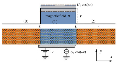
(a)

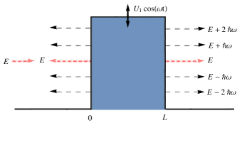
(b)

Figure 1: (color online) (a): Profile of a magnetic barrier driven by a periodic potential with frequency $\omega$, amplitude $U_{1}$, width $L$ and height $V$ applied to graphene composed of three regions. (b): Schematic of potential barrier oscillating in time.

Based on the results presented in Appendix A, we summarize our main solutions by writing the scattering states in different regions. Recall that, in regions 0 and 2 the potential height is $u_{j}=0$, then we proceed by replacing $J_{m-l}$ by $\delta_{ml}$. Consequently, we have in region 0 ($x<0$)

$$\psi_{\sf 0}(x,y,t)=e^{ik_{y}y}\sum^{+\infty}_{m,l=-\infty}\left[\delta_{l0}\left(\begin{array}[]{c}1\\ \alpha_{l}\end{array}\right)e^{ik_{l}x}+r_{l}\left(\begin{array}[]{c}1\\ -\frac{1}{\alpha_{l}}\end{array}\right)e^{-ik_{l}x}\right]\delta_{ml}\ e^{-iv_{F}(\epsilon+m\tilde{\omega})t}$$ (7)

and in region 2 $(x>L)$

$$\psi_{\sf 2}(x,y,t)=e^{ik_{y}y}\sum^{+\infty}_{m,l=-\infty}\left[t_{l}\left(\begin{array}[]{c}1\\ \beta_{l}\end{array}\right)e^{ik^{{}^{\prime}}_{l}x}+b_{l}\left(\begin{array}[]{c}1\\ -\frac{1}{\beta_{l}}\end{array}\right)e^{-ik^{{}^{\prime}}_{l}x}\right]\delta_{ml}\ e^{-iv_{F}(\epsilon+m\tilde{\omega})t}$$ (8)

where $\{b_{l}\}$ is a set of the null vectors, $\{r_{l}\}$ and $\{t_{l}\}$ are the reflection and transmission coefficients, respectively.

As far as region 1 ($0\leq x\leq L$) is concerned, where $H_{\sf II}$ is non zero, and according to [2] the eigenspinors $\psi_{\sf 1}(x,y,t)$ of the total Hamiltonian (1) can be expressed in terms of the eigenspinors $\psi_{1}(x,y)$ at energy $\epsilon$ of $H_{\sf I}$. Then, we have

$${\psi_{\sf 1}(x,y,t)=\psi_{1}(x,y)\sum^{+\infty}_{m=-\infty}J_{m}\left(\frac{u_{j}}{\tilde{\omega}}\right)\ e^{-iv_{F}(\epsilon+\tilde{\omega}m)t}}$$ (9)

where $J_{m}\left(\frac{u_{j}}{\tilde{\omega}}\right)$ are Bessel functions. We should emphasis that (9) is found by resolving the Schrödinger equation and requiring that the function $f=\sum_{m}J_{m}\left(\frac{u_{j}}{\tilde{\omega}}\right)e^{-im\omega t}$ must fulfill the condition $f^{\prime}=H_{\sf II}f$. To include all modes, a linear combination of spinors at energies $\epsilon+l\tilde{\omega}$ $(l=0,\pm 1,\cdots)$ has to be taken. Hence, one has to write (9) as

$$\psi_{\sf 1}(x,y,t)=\sum^{+\infty}_{l=-\infty}\psi_{l}(x,y)\sum^{+\infty}_{m=-\infty}J_{m}\left(\frac{u_{j}}{\tilde{\omega}}\right)\ e^{-iv_{F}(\epsilon+\tilde{\omega}(l+m))t}$$ (10)

such that the eigenspinors $\psi_{l}(x,y)$ are solution of the following equation

$$H\psi_{l}(x,y)={{v_{F}}}(\epsilon+l\tilde{\omega})\psi_{l}(x,y)$$ (11)

and the Hamiltonian is given by

$$H=v_{F}\left(\begin{array}[]{cc}m^{+}&-i\frac{\sqrt{2}}{l_{B}}a^{-}\\ i\frac{\sqrt{2}}{l_{B}}a^{+}&m^{-}\\ \end{array}\right)$$ (12)

where the shell operators for one mode

$$a^{\pm}=\frac{l_{B}}{\sqrt{2}}\left(\mp\partial_{x}+k_{y}+\frac{x}{l_{B}^{2}}\right)$$ (13)

are satisfying the canonical commutation relation $[a^{-},a^{+}]=\mathbb{I}$, where we have defined the parameters $m^{\pm}=v\pm\tilde{\Delta}$ by rescaling the potential $v=V/v_{F}$ and energy gap $\tilde{\Delta}=\Delta/v_{F}$, $l_{B}=\frac{1}{\sqrt{B_{0}}}$ is the magnetic length in the unit system $(\hbar=c=e=1)$. We determine the eigenvalues and eigenspinors of the Hamiltonian (12) by considering the time-independent equation for the spinor $\psi_{l}(x,y)=(\psi_{l}^{+},\psi_{l}^{-})^{T}$ using the fact that the transverse momentum $p_{y}$ is conserved to write $\psi_{l}(x,y)=e^{ip_{y}y}\varphi_{l}(x)$ with $\varphi_{l}(x)=(\varphi_{l}^{+},\varphi_{l}^{-})^{T}$. Then, the eigenvalue equation

$$H\left(\begin{array}[]{c}\varphi_{l}^{+}\\ \varphi_{l}^{-}\\ \end{array}\right)={{v_{F}}}(\epsilon+l\tilde{\omega})\left(\begin{array}[]{c}\varphi_{l}^{+}\\ \varphi_{l}^{-}\\ \end{array}\right)$$ (14)

gives the coupled equations

$$m^{+}\varphi_{l}^{+}-i\frac{\sqrt{2}}{l_{B}}a^{-}\varphi_{l}^{-}=(\epsilon+l\tilde{\omega})\varphi_{l}^{+}$$ (15)

$$i\frac{\sqrt{2}}{l_{B}}a^{+}\varphi_{l}^{+}+m^{-}\varphi_{l}^{-}=(\epsilon+l\tilde{\omega})\varphi_{l}^{-}.$$ (16)

Inserting (16) into (15) we end up with a differential equation of second order for $\varphi_{l}^{+}$

$$(\epsilon+l\tilde{\omega}-m^{+})(\epsilon+l\tilde{\omega}-m^{-})\varphi_{l}^{+}=\frac{2}{l_{B}^{2}}a^{-}a^{+}\varphi_{l}^{+}$$ (17)

which is in fact the equation of a harmonic oscillator and therefore we identify $\varphi_{l}^{+}$ with its eigenstates $|n_{l}-1\rangle$ corresponding to the eigenvalues

$$\tilde{\varepsilon}_{l}=\frac{1}{l_{B}}\sqrt{(\tilde{\Delta}l_{B})^{2}+2n_{l}}$$ (18)

where we have set $\tilde{\varepsilon}_{l}=s^{\prime}_{l}(\epsilon+l\tilde{\omega}-v)$, $s^{\prime}_{l}=\mbox{sign}(\epsilon+l\tilde{\omega}-v)$ correspond to positive and negative energy solutions. The second spinor component can be derived from (16) to obtain

$$\varphi_{l}^{-}=s^{\prime}_{l}i\sqrt{\frac{\tilde{\varepsilon}_{l}l_{B}-s^{\prime}_{l}\tilde{\Delta}l_{B}}{\tilde{\varepsilon}_{l}l_{B}+s^{\prime}_{l}\tilde{\Delta}l_{B}}}\mid n_{l}\rangle.$$ (19)

Introducing the parabolic cylinder functions $D_{n_{l}}(x)=2^{-\frac{n_{l}}{2}}e^{-\frac{x^{2}}{4}}H_{n_{l}}\left(\frac{x}{\sqrt{2}}\right)$ we express the solution in region 1 as

$$\psi_{\sf 1}(x,y,t) = e^{ik_{y}y}\sum^{+\infty}_{m,l=-\infty}\sum_{\pm}c^{\pm}_{l}\left(\begin{array}[]{c}f_{l}D_{\left(\left(\tilde{\varepsilon}_{l}l_{B}\right)^{2}-(\tilde{\Delta}l_{B})^{2}\right)/2-1}\left(\pm\sqrt{2}\left(\frac{x}{l_{B}}+k_{y}l_{B}\right)\right)\\ \pm i\tilde{f}_{l}D_{\left(\left(\tilde{\varepsilon}_{l}l_{B}\right)^{2}-\left(\tilde{\Delta}l_{B}\right)^{2}\right)/2}\left(\pm\sqrt{2}\left(\frac{x}{l_{B}}+k_{y}l_{B}\right)\right)\\ \end{array}\right)$$ (23)

$$J_{m-l}\left(\frac{u_{j}}{\tilde{\omega}}\right)e^{-iv_{F}(\epsilon+m\tilde{\omega})t}$$

where we have set

$$f_{l}=\sqrt{\frac{\tilde{\varepsilon}_{l}l_{B}+s^{\prime}_{l}\tilde{\Delta}l_{B}}{\tilde{\varepsilon}_{l}l_{B}}},\qquad\tilde{f}_{l}=\frac{s^{\prime}_{l}\sqrt{2}}{\sqrt{\tilde{\varepsilon}_{l}l_{B}\left(\tilde{\varepsilon}_{l}l_{B}+s^{\prime}_{l}\tilde{\Delta}l_{B}\right)}}.$$ (24)

The above solutions will be used to compute some physical quantities in our system such that the transmission probabilities and the associated GH shifts.

3 GH shifts for sidebands

Note that for our system, as Dirac particles pass through a region subject to time-harmonic potential, transitions from the central band to sidebands (channels) at energies $\epsilon\pm l\tilde{\omega}$ $(l=0,1,2,\cdots)$ occur as particles ex-change energy quanta with the oscillating field. Then to handle wave propagation, we need to evaluate the transmission and reflection amplitudes, which can be determined by matching different wave functions at interfaces $0$ and $L$. We write the continuity conditions

$$\psi_{\sf 0}(0,y,t)=\psi_{\sf 1}(0,y,t),\qquad\psi_{\sf 1}(L,y,t)=\psi_{\sf 2}(L,y,t).$$ (25)

To simplify the notation, we use the following shorthand expressions

$$\eta_{1,l}^{\pm}=D_{\frac{\left(\tilde{\varepsilon}_{l}l_{B}\right)^{2}-\left(\tilde{\Delta}l_{B}\right)^{2}}{2}-1}\left(\pm\sqrt{2}k_{y}l_{B}\right)$$ (26)

$$\xi_{1,l}^{\pm}=D_{\frac{\left(\tilde{\varepsilon}_{l}l_{B}\right)^{2}-\left(\tilde{\Delta}l_{B}\right)^{2}}{2}}\left(\pm\sqrt{2}k_{y}l_{B}\right)$$ (27)

$$\eta_{2,l}^{\pm}=D_{\frac{\left(\tilde{\varepsilon}_{l}l_{B}\right)^{2}-\left(\tilde{\Delta}l_{B}\right)^{2}}{2}-1}\left[\pm\sqrt{2}\left(\frac{L}{l_{B}}+k_{y}l_{B}\right)\right]$$ (28)

$$\xi_{2,l}^{\pm}=D_{\frac{\left(\tilde{\varepsilon}_{l}l_{B}\right)^{2}-\left(\tilde{\Delta}l_{B}\right)^{2}}{2}}\left[\pm\sqrt{2}\left(\frac{L}{l_{B}}+k_{y}l_{B}\right)\right].$$ (29)

To derive different physical quantities, one can explicitly write (25) making use the fact that the basis $\{e^{imv_{F}\tilde{\omega}t}\}$ is orthogonal. Thus at the interface $x=0$, one finds

$$\delta_{m0}+r_{m}=\sum^{+\infty}_{l=-\infty}\left(c^{+}_{l}f_{l}\eta_{1,l}^{+}+c^{-}_{l}f_{l}\eta_{1,l}^{-}\right)J_{m-l}\left(\frac{u_{j}}{\tilde{\omega}}\right)$$ (30)

$$\delta_{m0}\alpha_{m}-r_{m}\frac{1}{\alpha_{m}}=\sum^{+\infty}_{l=-\infty}\left(c^{+}_{l}i\tilde{f}_{l}\xi_{1,l}^{+}-c^{-}_{l}i\tilde{f}_{l}\xi_{1,l}^{-}\right)J_{m-l}\left(\frac{u_{j}}{\tilde{\omega}}\right)$$ (31)

and at $x=L$, we have

$$t_{m}e^{ik^{{}^{\prime}}_{m}d}+b_{m}e^{-ik^{{}^{\prime}}_{m}d}=\sum^{+\infty}_{l=-\infty}\left(c^{+}_{l}f_{l}\eta_{2,l}^{+}+c^{-}_{l}f_{l}\eta_{2,l}^{-}\right)J_{m-l}\left(\frac{u_{j}}{\tilde{\omega}}\right)$$ (32)

$$t_{m}\beta_{m}e^{ik^{{}^{\prime}}_{m}d}-b_{m}\frac{1}{\beta_{m}}e^{-ik^{{}^{\prime}}_{m}d}=\sum^{+\infty}_{l=-\infty}\left(c^{+}_{l}i\tilde{f}_{l}\xi_{2,l}^{+}-c^{-}_{l}i\tilde{f}_{l}\xi_{2,l}^{-}\right)J_{m-l}\left(\frac{u_{j}}{\tilde{\omega}}\right).$$ (33)

It is convenient to write (30-33) in matrix form

$$\left(\begin{array}[]{c}\Xi_{0}\\ \Xi_{0}^{{}^{\prime}}\\ \end{array}\right)=\left(\begin{array}[]{cc}{\mathbb{M}11}&{\mathbb{M}12}\\ {\mathbb{M}21}&{\mathbb{M}22}\\ \end{array}\right)\left(\begin{array}[]{c}\Xi_{2}\\ \Xi_{2}^{{}^{\prime}}\\ \end{array}\right)={\mathbb{M}}\left(\begin{array}[]{c}\Xi_{2}\\ \Xi_{2}^{{}^{\prime}}\\ \end{array}\right)$$ (42)

such that ${\mathbb{M}}={\mathbb{M}(0,1)}\cdot{\mathbb{M}(1,2)}$ and ${\mathbb{M}(j,j+1)}$ are transfer matrices that couple the wave function in the $j$-th region to the wave function in the $(j+1)$-th region, with

$${\mathbb{M}(0,1)}=\left(\begin{array}[]{cc}{\mathbb{I}}&{\mathbb{I}}\\ {\mathbb{N}_{1}^{+}}&{\mathbb{N}_{1}^{-}}\\ \end{array}\right)^{-1}\left(\begin{array}[]{cc}{\mathbb{C}_{1}^{+}}&{\mathbb{C}_{1}^{-}}\\ {\mathbb{G}_{1}^{+}}&{\mathbb{G}_{1}^{-}}\\ \end{array}\right)$$ (47)

$${\mathbb{M}(1,2)}=\left(\begin{array}[]{cc}{\mathbb{C}_{2}^{+}}&{\mathbb{C}_{2}^{-}}\\ {\mathbb{G}_{2}^{+}}&{\mathbb{G}_{2}^{-}}\\ \end{array}\right)^{-1}\left(\begin{array}[]{cc}{\mathbb{I}}&{\mathbb{I}}\\ {\mathbb{N}_{2}^{+}}&{\mathbb{N}_{2}^{-}}\\ \end{array}\right)\left(\begin{array}[]{cc}{\mathbb{K}^{+}}&{\mathbb{O}}\\ {\mathbb{O}}&{\mathbb{K}^{-}}\\ \end{array}\right)$$ (54)

where we have defined the quantities

$$\left({\mathbb{N}_{1}^{\pm}}\right)_{m,l}=\pm\left(\alpha_{m}\right)^{\pm 1}\delta_{ml}$$ (55)

$$\left({\mathbb{C}_{\tau}^{\pm}}\right)_{m,l}=f_{l}\eta_{\tau,l}^{\pm}J_{m-l}\left(\frac{u_{j}}{\tilde{\omega}}\right)$$ (56)

$$\left({\mathbb{G}_{\tau}^{\pm}}\right)_{m,l}=\pm i\tilde{f}_{l}\xi_{\tau,l}^{\pm}J_{m-l}\left(\frac{u_{j}}{\tilde{\omega}}\right)$$ (57)

$$\left({\mathbb{K}^{\pm}}\right)_{m,l}=\pm e^{\pm idk_{m}^{{}^{\prime}}}\delta_{ml}$$ (58)

$$\left({\mathbb{N}_{2}^{\pm}}\right)_{m,l}=\pm\left(\beta_{m}\right)^{\pm 1}\delta_{ml}$$ (59)

with the null matrix denoted by ${\mathbb{O}}$ and ${\mathbb{I}}$ is the unit matrix. We assume a particle propagating from left to right with energy $\epsilon$ then $\tau=(1,2)$, $\Xi_{0}=\{\delta_{0l}\}$ and $\Xi_{2}^{{}^{\prime}}=\{b_{m}\}$ is the null vector, whereas the vectors for wave transmission and reflection are $\Xi_{2}=\{t_{l}\}$, and $\Xi_{0}^{{}^{\prime}}=\{r_{l}\}$, respectively. From the above considerations, one can easily obtain the relation $\Xi_{2}=\left({\mathbb{M}11}\right)^{-1}\cdot\Xi_{0}$. The minimum number $N$ of sidebands that need to be considered is determined by the strength of the oscillation frequency, $N>\frac{u_{j}}{\tilde{\omega}}$, and the infinite series for $T$ can then be truncated to consider a finite number of terms starting from $-N$ up to $N$. Furthermore, analytical results are obtained if we take small values of $\frac{u_{j}}{\tilde{\omega}}$ and include only the first two sidebands at energies $\epsilon\pm\tilde{\omega}$ along with the central band at energy $\epsilon$, such as

$$t_{-N+k}={\mathbb{M}^{{}^{\prime}}}\left[k+1,N+1\right]$$ (60)

where $k=0,1,2,\cdots,2N$ and ${\mathbb{M}^{{}^{\prime}}}$ is a matrix element of $\left({\mathbb{M}11}\right)^{-1}$.

In the forthcoming analysis we truncate (60) retaining only the terms corresponding to the central and first two sidebands, namely $l=0,\pm 1$. This is justified for the driving amplitudes we consider because they are weak enough so that this approximation does not break. We can proceed as before to derive transmission amplitudes

$$t_{-1}={\mathbb{M}^{{}^{\prime}}}[1,2],\qquad t_{0}={\mathbb{M}^{{}^{\prime}}}[2,2],\qquad t_{1}={\mathbb{M}^{{}^{\prime}}}[3,2].$$ (61)

Now for a null amplitude of oscillating potential ($U_{j}=v_{F}u_{j}=0$), we get only the transmission amplitude $t_{0}$ for the central band. It can be calculated as

$$t_{0}=\rho_{0}e^{i\varphi^{t}_{0}}=\frac{i2f_{0}\tilde{f}_{0}\cos\phi_{0}}{e^{idk^{{}^{\prime}}_{0}}\left(\chi_{0}-if_{0}\tilde{f}_{0}\Omega_{0}\right)}\left(\eta^{+}_{2,0}\xi^{-}_{2,0}+\eta^{-}_{2,0}\xi^{+}_{2,0}\right)$$ (62)

where the phase shift $\varphi^{t}_{0}=\arctan\left(i\frac{t^{\ast}_{0}-t_{0}}{t^{\ast}_{0}+t_{0}}\right)$, $\rho_{0}=\sqrt{\mbox{Im}[t]^{2}+\mbox{Re}[t]^{2}}$ and different quantities are

$$\chi_{0}=f^{2}_{0}\left(\eta^{+}_{1,0}\eta^{-}_{2,0}-\eta^{-}_{1,0}\eta^{+}_{2,0}\right)e^{i\left(\theta_{0}-\phi_{0}\right)}-\tilde{f}^{2}_{0}\left(\xi^{+}_{1,0}\xi^{-}_{2,0}-\xi^{-}_{1,0}\xi^{+}_{2,0}\right)$$ (63)

$$\Omega_{0}=\left(\left(\eta^{+}_{2,0}\xi^{-}_{1,0}+\eta^{-}_{2,0}\xi^{+}_{1,0}\right)e^{i\theta_{0}}+\left(\eta^{+}_{1,0}\xi^{-}_{2,0}+\eta^{-}_{1,0}\xi^{+}_{2,0}\right)e^{-i\phi_{0}}\right).$$ (64)

As a result, the transmission probabilities are finally expressed as

$$T_{l}=\frac{k^{{}^{\prime}}_{l}}{k_{0}}\rho_{l}^{2},\qquad l=0,\pm 1.$$ (65)

The Goos-Hänchen (GH) shifts in graphene can be analyzed by considering the incident, reflected and transmitted beams around some transverse wave vector $k_{y}=k_{y_{0}}$ together with the angle of incidence $\phi_{l}(k_{y_{0}})\in[0,\frac{\pi}{2}]$, denoted by the subscript $0$. These can be expressed in integral forms for incident

$$\Psi_{in}(x,y) = \int_{-\infty}^{+\infty}dk_{y}\ f(k_{y}-k_{y_{0}})\ e^{i(k_{0}(k_{y})x+k_{y}y)}\begin{pmatrix}{1}\\ {e^{i\phi_{0}(k_{y})}}\end{pmatrix}$$ (66)

and reflected beams

$$\Psi_{re}(x,y) = \int_{-\infty}^{+\infty}dk_{y}\ r_{l}(k_{y})\ f(k_{y}-k_{y_{0}})\ e^{i(-k_{l}(k_{y})x+k_{y}y)}\begin{pmatrix}{1}\\ {-e^{-i\phi_{l}(k_{y})}}\\ \end{pmatrix}$$ (67)

where the reflection amplitude is defined by $r_{l}(k_{y})=|r_{l}|e^{i\varphi_{l}^{r}}$. This result is reached by writing the $x$-component of wave vector $k_{l}$ as well as $\phi_{l}$ in terms of $k_{y}$ such that each spinor plane wave is a solution of (1) and $f(k_{y}-k_{y_{0}})$ is the angular spectral distribution. We can approximate the $k_{y}$-dependent terms by a Taylor expansion around $k_{y}$, retaining only the first order term to get

$$\phi_{l}(k_{y})\approx\phi_{l}(k_{y_{0}})+\frac{\partial\phi_{l}}{\partial k_{y}}\Big{|}_{k_{y_{0}}}(k_{y}-k_{y_{0}})$$ (68)

$$k_{l}(k_{y})\approx k_{l}(k_{y_{0}})+\frac{\partial k_{l}}{\partial k_{y}}\Big{|}_{k_{y_{0}}}(k_{y}-k_{y_{0}}).$$ (69)

Finally, the transmitted beams are

$$\Psi_{tr}(x,y) = \int_{-\infty}^{+\infty}dk_{y}\ t_{l}(k_{y})\ f(k_{y}-k_{y_{0}})\ e^{i(k^{{}^{\prime}}_{l}(k_{y})x+k_{y}y)}\begin{pmatrix}{1}\\ {e^{i\theta_{l}(k_{y})}}\\ \end{pmatrix}$$ (70)

where the transmission coefficient is $t_{l}(k_{y})=|t_{l}|e^{i\varphi_{l}^{t}}$.

The stationary-phase approximation indicates that the GH shifts are equal to the negative gradient of transmission phase with respect to $k_{y}$. To calculate the GH shifts of the transmitted beams through our system, according to the stationary phase method [22], we adopt the definition [9, 23]

$$S_{l}^{t}=-\frac{\partial\varphi_{l}^{t}}{\partial k_{y}}\Big{|}_{k_{y_{0}}},\qquad S_{l}^{r}=-\frac{\partial\varphi_{l}^{r}}{\partial k_{y}}\Big{|}_{k_{y_{0}}}.$$ (71)

Assuming a finite-width beam with a Gaussian shape, $f(k_{y}-k_{y_{0}})=w_{y}\exp[-w_{y}^{2}(k_{y}-k_{y_{0}})^{2}]$ around $k_{y_{0}}$, where $w_{y}=w\sec\phi_{l}$, and $w$ is the half beam width at waist. We can now evaluate the Gaussian integral to obtain the spatial profile of the incident beam, by expanding $\phi_{l}$ and $k_{l}$ to first order around $k_{y_{0}}$ while satisfying the condition $\delta\phi_{l}=\lambda_{F}/(\pi w)\ll 1$ where $\lambda_{F}$ is the Fermi wavelength. Comparison of the incident and transmitted beams suggests that the displacements $\sigma_{\pm}$ of up and down spinor components are both equal to $\partial\varphi_{l}^{t}/\partial k_{y_{0}}$ and the average displacement is

$$S_{l}^{t}=\frac{1}{2}(\sigma^{+}+\sigma^{-})=-\frac{\partial\varphi_{l}^{t}}{\partial k_{y}}\Big{|}_{k_{y_{0}}}.$$ (72)

It should be noted that when the above-mentioned condition is satisfied, that is, the stationary phase method is valid [9], the definition (71) can be applied to any finite-width beam, the shape does not necessarily need to be Gaussian-shaped.

4 Results and Discussions

In this section, we study the effect of the magnetic field on the Goos-Hänchen (GH) shifts for Dirac fermions in gaped graphene that is subject to an additional time periodic oscillating potential in the region of space with the potential barrier. We numerically evaluate the GH shifts in transmission for the central band $S_{0}^{t}$ and two first sidebands $S_{\pm 1}^{t}$ as a function of the parameters of the graphene single barrier oscillation frequency $\tilde{\omega}l_{B}$ and amplitude $\frac{u_{j}}{\tilde{\omega}}$, in addition to the energy $\epsilon l_{B}$, the $y$-component of the wave vector $k_{y}l_{B}$, the energy gap $\tilde{\Delta}l_{B}$ and the strength of static potential barrier $vl_{B}$. To understand these effects, let us consider Figure 2 where we study the GH shifts in transmission versus the potential barrier $vl_{B}$ in the gapless graphene region where $\tilde{\Delta}l_{B}=0$, the frequency $\tilde{\omega}l_{B}=1$, and the energy $\epsilon l_{B}=10$, $k_{y}l_{B}=2$, $\frac{L}{l_{B}}=0.8$. Figure 2a shows the GH shifts in transmission for the central band $S_{0}^{t}$ (red line) and first two sidebands $S_{-1}^{t}$ (green line), $S_{1}^{t}$ (blue line) where the value $\frac{u_{j}}{\tilde{\omega}}=0.4$, the GH shifts in transmission changes sign at the Dirac points $vl_{B}=\epsilon l_{B}+l\tilde{\omega}$ ($l=0$ for band central and $l=\pm 1$ for first two sidebands). It is clearly seen that they are strongly dependent on the barrier heights and frequency $\tilde{\omega}l_{B}$. Figure 2b shows the GH shifts in transmission for the central band for different values of $\frac{u_{j}}{\tilde{\omega}}=\{0,0.45,0.85\}$. One can notice that, at the Dirac points $vl_{B}=\epsilon l_{B}$, the GH shifts change their sign. We observe that the GH shifts for central band $S_{0}^{t}$ in the oscillating barrier decreases if $\frac{u_{j}}{\tilde{\omega}}$ increases. We also notice that the GH shifts can have either sign, positive and negative in Figures 2a and 2b.

(a)

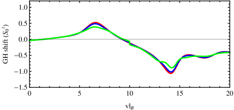
(b)

Figure 2: (color online) The GH shifts in transmission as a function of $vl_{B}$ with $k_{y}l_{B}=2$, $\frac{L}{l_{B}}=0.8$, $\tilde{\omega}l_{B}=1$ $\tilde{\Delta}l_{B}=0$ and $\epsilon l_{B}=10$. (a): Central band $S_{0}^{t}$ in red, the first two sidebands $S_{1}^{t}$ in blue and $S_{-1}^{t}$ in green with $\alpha=0.4$. (b): Central band $S_{0}^{t}$. For different values of $\frac{u_{j}}{\tilde{\omega}}$: 0 (red line), $0.45$ (blue line), $0.85$ (green line).

Now let us investigate what happens if we introduce a gap in the intermediate region $0\leq x\leq L$, which is also subjected to a magnetic field. Note that, the gap is introduced as shown in Figure 1 and therefore it affects the system energy according to the solution of the energy spectrum obtained in region $1$. From (18), we obtain the energy modulation due the oscillating potential as shown in Figure 3 as function of the magnetic field $B$ with $v=30$, $w=10$, $l=${-1: (color dot-dashed), 0: (color thick), 1: (color dashed)} and $n=${0: (blue line), 1: (red line), 2: (green line)} for gapless $\tilde{\Delta}=0$ in Figure 3a and gap $\tilde{\Delta}=10$ in Figure 3b. It is clearly seen that the difference of energy is $\epsilon(n+1;l)-\epsilon(n;l)=\tilde{\omega}$, which is independent of the quantum number $n$. For $n=0$, we have just a modulation of the energy with different quantum number $l\tilde{\omega}$ with $l=0,\pm 1$. However for $n=1,2$ the energy behavior is completely changed and for each $l$ value the energy is split into two values, which can be seen like a left of degeneracy of levels. It is clearly seen that absorbing energy quantum $\tilde{\omega}$ produces inter-level transitions. Because of Pauli principle a particle with energy $\epsilon$ can absorb an energy quantum $\tilde{\omega}$ if and only if the state with energy $\epsilon+\tilde{\omega}$ is empty. We observe that in Figure 3b the difference of energy $\epsilon^{+}$ and $\epsilon^{-}$ for quantum number $n=0$ and the value $l=0,\pm 1$ is $\epsilon^{+}(n=0;l=0,\pm 1)-\epsilon^{-}(n=0;l=0,\pm 1)=2\tilde{\Delta}$. The difference of energy $\epsilon^{+}$ and $\epsilon^{-}$ for quantum number $n=1,2$ and the value $l=0,\pm 1$ is $\epsilon^{+}(n=1,2;l=0,\pm 1)-\epsilon^{-}(n=1,2;l=0,\pm 1)=2(\tilde{\Delta}+\mu_{n})$ with $\mu_{n}=\epsilon^{+}(n=1,2;l=0,\pm 1)-\epsilon^{+}(n=0;l=0,\pm 1)$.

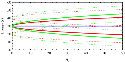
(a) $\tilde{\Delta}=0$

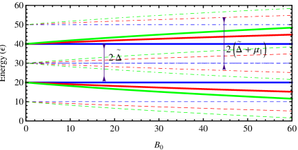
(b) $\tilde{\Delta}=10$

Figure 3: (color online) Graphs depicting the energy $\epsilon$ as a function of magnetic field $B$ with the energy gap (a): $\tilde{\Delta}=0$ and (a): $\tilde{\Delta}=10$. For the frequency $\tilde{\omega}=10$, potential $v=30$, quantum number $n=0$ (blue line), $n=1$ (red line), $n=2$ (green line) and the modes $l=0$ (color thick), $l=1$ (color dashed), $l=-1$ (color dot-dashed).

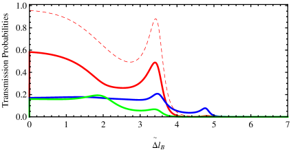
(a)

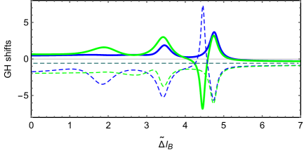
(b)

Figure 4: (color online) (a): The transmission probabilities $T_{l}$ for central band and first tow sidebands and (b): GH shifts in transmission $S_{\pm 1}^{t}$ for first tow sidebands as a function of energy gap $\tilde{\Delta}l_{B}$ with $\frac{u_{j}}{\tilde{\omega}}=0$ (not oscillating barrier), $\frac{u_{j}}{\tilde{\omega}}=0.65$ (oscillating barrier), $k_{y}l_{B}=2$, $\frac{L}{l_{B}}=1.4$, $\tilde{\omega}l_{B}=1$ and ($\{\epsilon l_{B}=12;vl_{B}=7\})/(\{\epsilon l_{B}=12;vl_{B}=7\},\{\epsilon l_{B}=7;vl_{B}=12\}$). For no oscillating barrier $T_{0}$ (red dashed) and for oscillating barrier $T_{0}$ (red line), $T_{-1}$ (green line), $T_{1}$ (blue line).

In Figure 4 we present the transmission probabilities $T_{l}$ for the central band and first two sidebands together with the GH shifts in transmission $S_{\pm 1}^{t}$ for first two sidebands as a function of the energy gap $\tilde{\Delta}l_{B}$ for $\frac{u_{j}}{\tilde{\omega}}=0.65$ (oscillating magnetic barrier) along with the results for a static barrier and specific values $k_{y}l_{B}=2$, $\frac{L}{l_{B}}=1.4$, $\tilde{\omega}l_{B}=1$. In Figure 4a for $\frac{u_{j}}{\tilde{\omega}}=0,65$, we observe that the maximum value of $T_{0}$ decreases at the expense of transmission sidebands $T_{\pm 1}$. We notice that the sum of the three transmissions $T_{0,-1,1}$ converges whenever towards transmission $T_{0}$ for $\frac{u_{j}}{\tilde{\omega}}=0$. In fact, under the condition $\tilde{\Delta}l_{B}>|\epsilon l_{B}+l\tilde{\omega}l_{B}-vl_{B}|$ every incoming state is fully reflected. In Figure 4b, the GH shifts $S_{\pm 1}^{t}$ in transmission for first two sidebands in the propagating case can be enhanced by opening a gap at the Dirac point. This computation has been performed keeping the parameters $\frac{u_{j}}{\tilde{\omega}}=0.65$, $k_{y}l_{B}=2$, $\frac{L}{l_{B}}=1.4$, $\tilde{\omega}l_{B}=1$ and making different choices for the energy $\epsilon l_{B}$ and potential $vl_{B}$. For the configuration $\{\epsilon l_{B}=12,vl_{B}=7\}$, we can still have positive shifts while for configuration $\{\epsilon l_{B}=7,vl_{B}=12\}$ the GH shifts are negative. The GH shifts in transmission for the first two sidebands $S_{1}^{t}$ (blue line) and $S_{-1}^{t}$ (green line) did not vanish and decrease with increasing $\tilde{\Delta}l_{B}$ for $s=\text{sign}(\epsilon l_{B}-vl_{B})=-1$ as well as increases with increasing $\tilde{\Delta}l_{B}$ for $s=\text{sign}(\epsilon l_{B}-vl_{B})=1$. It is clearly seen that the GH shifts can be enhanced by a certain gap opening. Indeed, by increasing the gap we observe that the gap of transmission becomes broader, changing the transmission resonances and the modulation of the GH shifts. Note that for a certain energy gap $\tilde{\Delta}l_{B}$, there is total reflection and therefore the GH shifts in transmission $S_{\pm 1}^{t}$ do not vanish.

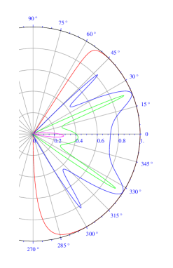
(a)

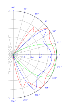
(b)

Figure 5: (color online) Polar graphs depicting the transmission probability $T_{0}(\phi_{0})$ for a magnetic barrier of $\frac{u_{j}}{\tilde{\omega}}=0$ with $\frac{L}{l_{B}}=1.2$, $vl_{B}=0$. (a): For various gap $\tilde{\Delta}l_{B}=\{0,4,6,7.1\}$ and $\epsilon l_{B}=7.5$. (b): For various energy $\epsilon l_{B}=\{1.8,3.5,5,7.5\}$ and $\tilde{\Delta}l_{B}=2$.

In Figure 5, we plot the transmission probabilities in central band $T_{0}$ for magnetic barrier $\frac{u_{j}}{\tilde{\omega}}=0$ as a function of the incidence angle $\phi_{0}$ for specific values of $\frac{L}{l_{B}}=1.2$, $vl_{B}=0$. We show that it is possible to confine massless Dirac fermions in graphene sheet by inhomogeneous magnetic field and the induced gap $\tilde{\Delta}$. The outermost circle corresponds to full transmission total $T_{0}=1$, while the origin of this plot represents zero transmission $T_{0}=0$. In Figure 5a we show how the transmission is affected by the effective mass term reflected by $\tilde{\Delta}l_{B}=\{0,4,6,7.1\}$ and the parameters $\epsilon l_{B}=7.5$, the transmission decreases sharply as we increase the energy gap $\tilde{\Delta}l_{B}$, there is no transmission possible. We notice that for certain incidence angles the transmission is not allowed, in fact for $\epsilon l_{B}\leq L/l_{B}-l\tilde{\omega}l_{B}$ all waves are completely reflected. It is worth mentioning that the transmission is uniquely defined by the incidence angle $\phi_{0}$. Each radial line represents a given incidence angle and intersects the transmission curve at one point. In Figure 5b for the energy gap $\tilde{\Delta}l_{B}=2$ and various energy $\epsilon l_{B}=\{1.8,3.5,5,7.5\}$, we see that the transmission vanishes for $\epsilon l_{B}\leq 1.2$.

It is well known that graphene has a zero band gap because the Dirac-Weyl Hamiltonian, that models graphene, describes massless quasiparticles [24, 25] and hence allows for Klein tunneling. However, electronic components such as electronic switches, diodes and transistors, require that the current can be cut off/on. It is necessary then to induce an energy gap in graphene in order to control the current flow. Therefore, we also investigated the influence of the energy gap on the GH shifts in Figure 6 where $S_{l}^{t}$ for the central band and first two sidebands is plotted as a function of the potential $\epsilon l_{B}$ for $\frac{u_{j}}{\tilde{\omega}}=0.4$ and specific values $k_{y}l_{B}=2$, $\epsilon l_{B}=10$, $d/l_{B}=1.5$, $\tilde{\omega}l_{B}=1$, $\tilde{\Delta}l_{B}=1$, different energy gaps such that $\tilde{\Delta}l_{B}=1$ in Figure 6a and $\tilde{\Delta}l_{B}=3$ in Figure 6b. From these, we see that the region of weak GH shifts becomes wider with increased energy gap. Then, we can control the positive and negative GH shifts by changing the $y$-directional wave vector $k_{y}/l_{B}$ or the energy gap $\tilde{\Delta}l_{B}$. In other words, we can control the directions of the carriers at the interface of the graphene barrier by adjusting $k_{y}/l_{B}$ or $\tilde{\Delta}l_{B}$. The GH shifts still change sign and the absolute value of the maximum of the shifts increased as well. It is clearly seen that $S_{l}^{t}$ are oscillating between negative and positive values around the critical point $\epsilon l_{B}=vl_{B}-l\tilde{\omega}l_{B}$ $(l=0,\pm 1)$.

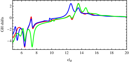
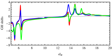
Figure 6: (color online) The GH shifts in transmission for central band and first tow sidebands as a function of the energy $\epsilon l_{B}$ for $\frac{u_{j}}{\tilde{\omega}}=0.4$, $k_{y}l_{B}=2$, $\epsilon l_{B}=10$, $\frac{L}{l_{B}}=1.5$, $\tilde{\omega}l_{B}=1$ with (a): $\tilde{\Delta}l_{B}=1$ and (b): $\tilde{\Delta}l_{B}=3$. $S_{0}^{t}$ (red line), $S_{-1}^{t}$ (green line), $S_{1}^{t}$ (blue line).

In Figure 7, we present the transmission probabilities $T_{l}$ and the GH shifts in transmission $S_{l}^{t}$ for the central band and first two sidebands as a function of the potential $vl_{B}$ for $\frac{u_{j}}{\tilde{\omega}}\neq 0$ (oscillating barrier) along with that for the static barrier $\frac{u_{j}}{\tilde{\omega}}=0$ and specific values $k_{y}l_{B}=2$, $\epsilon l_{B}=10$, $d/l_{B}=1.5$, $\tilde{\omega}l_{B}=1$, $\tilde{\Delta}l_{B}=1$, such that $\frac{u_{j}}{\tilde{\omega}}=0.4$ in Figure 7(a,c) and $\frac{u_{j}}{\tilde{\omega}}=0.85$ in Figure 7(b,d). Both quantities are showing a series of peaks and resonances where the resonances correspond to the bound states of the magnetic barrier for $\frac{u_{j}}{\tilde{\omega}}=0$ and the oscillating magnetic barrier for $\frac{u_{j}}{\tilde{\omega}}\neq 0$. We notice that the GH shifts in transmission peak at each bound state energy are clearly shown in the transmission curve underneath. The energies at which transmission vanishes correspond to energies at which the GH shifts in transmission change sign. Since these resonances are very sharp (true bound states with zero width) it is numerically very difficult to track all of them, if we do this then the alternation in sign of the GH shifts will be observed. We notice that around the Dirac point $vl_{B}=\epsilon l_{B}+l\tilde{\omega}l_{B}$ the number of peaks is equal to the number of transmission resonances. At such a point $T_{l}$ is showing transmission probabilities for the central band and the first two sidebands while it oscillates away from the critical point. We notice that for large values of $vl_{B}$, the GH shifts can be positive as well as negative. We deduce that there is a strong dependence of the GH shifts on the potential height $vl_{B}$, which can help to realize a controllable sign of the GH shifts. We also find that the quantity $\frac{u_{j}}{\tilde{\omega}}$ is very significant in determining the GH shifts and transmission probabilities for various sidebands as shown here. This is to be expected as the probabilities are now spread over the central band and sidebands. In addition, the maximum transmission through the oscillating barrier depends on the value of $\frac{u_{j}}{\tilde{\omega}}$.

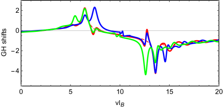
(a)

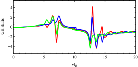
(b)

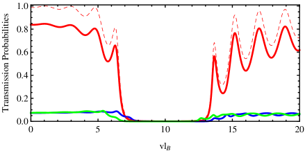
(c)

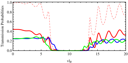
(d)

Figure 7: (color online) The GH shifts in transmission and transmission probabilities for central band and first tow sidebands as a function of the potential $vl_{B}$ for $\frac{u_{j}}{\tilde{\omega}}\neq 0$ (oscillating barrier) along with that for static barrier $\frac{u_{j}}{\tilde{\omega}}=0$, $k_{y}l_{B}=2$, $\epsilon l_{B}=10$, $\frac{L}{l_{B}}=1.5$, $\tilde{\omega}l_{B}=1$, $\tilde{\Delta}l_{B}=1$. (a)/(c): $\frac{u_{j}}{\tilde{\omega}}=0.4$ and (b)/(d): $\frac{u_{j}}{\tilde{\omega}}=0.85$. For no oscillating barrier $(T_{0},S_{0}^{t})$ (red dashed) and for oscillating barrier $(T_{0},S_{0}^{t})$ (red line), $(T_{-1},S_{-1}^{t})$ (green line), $(T_{1},S_{1}^{t})$ (blue line).

5 Conclusion

We have studied the effect of both time-oscillating scalar potential and magnetic field on the Goos-Hänchen (GH) shifts for the particle transport in gapped graphene. The solutions of energy spectrum are obtained in terms of the physical parameters. We have shown that the time-dependent oscillating barrier height generates additional sidebands at energies $\epsilon+l\tilde{\omega}$ in the transmission probability due to photon absorption or emission. We have observed that perfect transmission probability at normal incidence (Klein tunneling) persist for a harmonically driven single barrier.

We have also investigated how the GH shifts in transmission are affected by various parameters such that the incident angle of the particles, width and height of the barrier and oscillation frequency. Thus our numerical results support the assertion that quantum interference has an important effect on particle tunneling through a time-dependent graphene-based single barrier. The tunneling modes inside the gap and the corresponding positive and negative GH shifts are further analyzed. The GH shifts in transmission for central band and two first sidebands change sign at the Dirac points $vl_{B}=\epsilon l_{B}+l\tilde{\omega}{{l_{B}}}$. In particular, the GH shifts change sign at the transmission zero energies and peaks at each bound state associated with the single barrier. It is observed that the GH shifts can be enhanced by the presence of resonant energies in the system when the incident angle is less than the critical angle associated with total reflection.

Appendix A

To explicitly determine the energy spectrum in our theoretical model, we separately handle each part of the Hamiltonian (1). Thus, let us start from the time-independent Dirac equation in the absence of oscillating potential for the spinor $\psi(x,y)=(\psi_{+},\psi_{-})^{T}$ at energy $E$, such as

$$H_{\sf I}\psi(x,y,t)=E\psi(x,y,t)$$ (A.1)

where $\psi(x,y,t)=\psi(x,y)e^{-iEt/\hbar}$. In matrix form, we have

$$\left(\begin{array}[]{cc}0&-i\partial_{x}-\partial_{y}-\frac{ie}{\hbar c}A(x)\\ -i\partial_{x}+\partial_{y}+\frac{ie}{\hbar c}A(x)&0\\ \end{array}\right)\left(\begin{array}[]{c}\psi_{+}\\ \psi_{-}\\ \end{array}\right)=\frac{E}{\hbar\upsilon_{F}}\left(\begin{array}[]{c}\psi_{+}\\ \psi_{-}\\ \end{array}\right).$$ (A.2)

Since the transverse momentum $p_{y}$ is conserved, we can write the wave function in a separable form $\psi_{\pm}(x,y)=\varphi_{\pm}(x)e^{ik_{y}y}$. Thus after rescaling energy $\epsilon=E/v_{F}$ and using the unit system with $(\hbar=c=e=1)$, we obtain the two linear first order differential equations

$$\left(-i\partial_{x}-ik_{y}-iA(x)\right)\varphi_{-}=\epsilon\varphi_{+}$$ (A.3)

$$\left(-i\partial_{x}+ik_{y}+iA(x)\right)\varphi_{+}=\epsilon\varphi_{-}.$$ (A.4)

These can be combined to describe the solution of (A.2) and then consider the incoming particles to be in plane wave states $\psi_{inc}(x,y,t)$ at energy $\epsilon$ as

$$\psi_{inc}(x,y,t)=\begin{pmatrix}1\\ \alpha_{0}\end{pmatrix}e^{ik_{0}x}e^{ik_{y}y}e^{-iv_{F}\epsilon t}$$ (A.5)

such that $\alpha_{0}$ is given by

$$\alpha_{0}=s_{0}\frac{k_{0}+ik_{y}}{\sqrt{k_{0}^{2}+k_{y}^{2}}}=s_{0}e^{\textbf{\emph{i}}\phi_{0}}$$ (A.6)

where $s_{0}=\mbox{sgn}(\epsilon)$, $\phi_{0}$ is the angle that the incident particles make with the $x$-direction, $k_{0}$ and $k_{y}$ are the $x$ and $y$-components of the wave vector, respectively. After rescaling the potentials $V=v_{F}v$, $U_{j}=v_{F}u_{j}$ and frequency $\omega=v_{F}\tilde{\omega}$, we show that the transmitted and reflected waves have components at all energies $\epsilon+l\tilde{\omega}$ $(l=0,\pm 1,\cdots)$. Indeed the wave functions $\psi_{re}(x,y,t)$ for reflected electrons are

$$\psi_{re}(x,y,t)=\sum^{+\infty}_{m,l=-\infty}r_{l}\left(\begin{array}[]{c}1\\ -\frac{1}{\alpha_{l}}\end{array}\right)e^{-ik_{l}x+ik_{y}y}J_{m-l}\left(\frac{{{u_{j}}}}{\tilde{\omega}}\right)\ e^{-iv_{F}(\epsilon+m\tilde{\omega})t}$$ (A.7)

and the corresponding energy reads as

$$\epsilon+l\tilde{\omega}=s_{l}\sqrt{k^{2}_{l}+k^{2}_{y}}$$ (A.8)

where $r_{l}$ is the reflection amplitude and $J_{m}\left(\frac{u_{j}}{\tilde{\omega}}\right)$ is the Bessel function of the first kind. Note that for the modulation amplitude $u_{j}=0$ we have $J_{m-l}\left(0\right)=\delta_{ml}$. We will return to this point once we talk about the solution in different regions composing our system. The parameter $\alpha_{l}$ is the complex number

$$\alpha_{l}=s_{l}\frac{k_{l}+ik_{y}}{\sqrt{k^{2}_{l}+k_{y}^{2}}}=s_{l}\ e^{\textbf{\emph{i}}\phi_{l}}$$ (A.9)

where $\phi_{l}=\tan^{-1}(k_{y}/k_{l})$, $s_{l}=\mbox{sgn}(\epsilon+l\tilde{\omega})$, the sign again refers to conduction and valence bands regions. The (number) wavevector $k_{l}$ for mode $l$ can be obtained from (A.8) to end up with

$$k_{l}=s_{l}\sqrt{\left(\epsilon+l\tilde{\omega}\right)^{2}-k^{2}_{y}}.$$ (A.10)

While, the wave functions $\psi_{tr}(x,y,t)$ for transmitted electrons read as

$$\psi_{tr}(x,y,t)=\sum^{+\infty}_{m,l=-\infty}t_{l}\left(\begin{array}[]{c}1\\ \beta_{l}\end{array}\right)e^{ik^{{}^{\prime}}_{l}x+ik_{y}y}J_{m-l}\left(\frac{{{u_{j}}}}{\tilde{\omega}}\right)e^{-iv_{F}(\epsilon+m\tilde{\omega})t}$$ (A.11)

and the eigenvalues

$$\epsilon+l\tilde{\omega}=s_{l}\sqrt{k^{{}^{\prime}2}_{l}+\left(k_{y}+\frac{{{L}}}{l^{2}_{B}}\right)^{2}}$$ (A.12)

where the magnetic length $l_{B}=\sqrt{1/B_{0}}$, transmission amplitude $t_{l}$ and the next complex number

$$\beta_{l}=s_{l}\frac{k^{{}^{\prime}}_{l}+i\left(k_{y}+\frac{{{L}}}{l^{2}_{B}}\right)}{\sqrt{k^{{}^{\prime}2}_{l}+\left(k_{y}+\frac{{{L}}}{l^{2}_{B}}\right)^{2}}}=s_{l}\ e^{\textbf{\emph{i}}\theta_{l}}$$ (A.13)

$$k^{{}^{\prime}}_{l}=s_{l}\sqrt{\left(\epsilon+l\tilde{\omega}\right)^{2}-\left(k_{y}+\frac{{{L}}}{l^{2}_{B}}\right)^{2}}$$ (A.14)

$$\theta_{l}=\tan^{-1}\left[\left(k_{y}+\frac{{{L}}}{l^{2}_{B}}\right)/k^{{}^{\prime}}_{l}\right].$$ (A.15)

References

- [1] A. H. Dayem and R. J. Martin, Phys. Rev. Lett. 8, 246 (1962).
- [2] P. K. Tien and J. P. Gordon, Phys. Rev. 129, 647 (1963).
- [3] M. Moskalets and M. Buttiker, Phys. Rev. B 66, 035306 (2002).
- [4] A. Jellal, M. Mekkaoui, E. B. Choubabi, and H. Bahlouli, Eur. Phys. J. B 87, 123 (2014).
- [5] F. Grossmann, T. Dittrich, P. Jung, and P. Hanggi, Phys. Rev. Lett. 67, 516 (1991).
- [6] M. Wagner, Phys. Rev. B 49, 16544 (1994); Phys. Rev. A 51, 798 (1995).
- [7] F. Goos and H. Hänchen, Ann. Phys. 1, 333 (1947); ibid 5, 251 (1949).
- [8] K. Artmann, Ann. Physik 2, 87 (1949)
- [9] X. Chen, J.-W. Tao, and Y. Ban, Eur. Phys. J. B 79, 203 (2011).
- [10] Y. Song, H-C. Wu, and Y. Guo, Appl. Phys. Lett. 100, 253116 (2012).
- [11] X. Chen, P-L. Zhao, X-J. Lu, and L-G. Wang, Eur. Phys. J. B 86, 223 (2013).
- [12] A. Kamal and A. Jellal, Physica E 119, 114010 (2020).
- [13] M. Sharma and S. Ghosh, J. Phys.: Condens. Matter 23, 055501 (2011).
- [14] J.-H. Huang, Z.-L. Duan, H.-Y. Ling, and W.-P. Zhang, Phys. Rev. A 77, 063608 (2008).
- [15] C. W. J. Beenakker, R. A. Sepkhanov, A. R. Akhmerov, and J. Tworzydlo, Phys. Rev. Lett. 102, 146804 (2009).
- [16] L. Zhao and S. F. Yelin, Phys. Rev. B 81, 115441 (2010).
- [17] L. Jiang, J. Wu, X. Dai, and Y. Xiang, Optik 125, 7025 (2014).
- [18] L. Jiang, Q. Wang, Y. Xiang, X. Dai, and S. Wen, IEEE Photonics J. 5, (2013).
- [19] Q. You, L. Jiang, X. Dai, and Y. Xiang, Chinese Phys. B 27, 094211 (2018).
- [20] Q. You, Y. Shan, S. Gan, Y. Zhao, X. Dai, and Y. Xiang, Opt. Mater. Express 8, 3036 (2018).
- [21] B. Lemaalem, M. Mekkaoui, A. Jellal, and H. Bahlouli, Europhys. Lett. 129, 27001 (2020).
- [22] D. Bohm, Quantum Theory (Prentice-Hall, New York, 1951, pp. 257-261).
- [23] A. Jellal, Y. Wang, Y. Zahidi and M. Mekkaoui, Physica E 68, 53 (2015).
- [24] K. S. Novoselov, A. K. Geim, S. V. Morozov, D. Jiang, Y. Zhang, S. V. Dubonos, I. V. Grigorieva, and A. A. Firsov, Science 306, 666 (2004).
- [25] Y. Zhang, Y. W. Tan, H. L. Strömer, and P. Kim, Nature 438, 201 (2005).