Expectation and Price in Incomplete Markets

Abstract

Risk-neutral pricing dictates that the discounted derivative price is a martingale in a measure equivalent to the economic measure. The residual ambiguity for incomplete markets is here resolved by minimising the entropy of the price measure from the economic measure, subject to mark-to-market constraints, following arguments based on the optimisation of portfolio risk. The approach accounts for market and funding convexities and incorporates available price information, interpolating between methodologies based on expectation and replication.

The principal innovation of the financial derivatives industry is the ability to transform an arbitrary economic observable into a tradable financial instrument. Provided that this is measurable at or prior to settlement, the contractual terms dictate that the measurement of the observable becomes the terminal cash value of the corresponding derivative. Failure to deliver on the contract, and any other circumstances that alter the settlement amount, are absorbed in the definition of the reference observable, allowing default and external factors to be incorporated. This contractualisation of economic observables permits the future exchange of currencies in amounts that are undetermined at present.

The conceptual framework considered here assumes a universe of economic observables whose values are revealed progressively through time, which are then utilised as the cash settlement amounts for derivative securities in one or more idealised currencies. Liquidity constraints are not considered, and settlement is permitted in arbitrarily large positive or negative amounts. No other properties of the securities are investigated, and derivatives that match at settlement in all future scenarios are assumed to be fungible.

Figure 1: A sample term sheet for a ‘range accrual’ derivative. The term sheet describes the observations (Euribor EUR 6M fixing) and calculations (indicator function for a defined range) used to determine settlement amounts, together with the dates on which the payments will be made. Bilateral arrangements between the counterparties may prescribe further payments, such as margin and collateral exchanges. The trade is also subject to the terms of the legal jurisdiction, covering matters such as regulatory capital requirements and actions in the event of default. All these settlements related to the derivative potentially impact its valuation.

The price of the derivative must then account for discounting, the adjustment due to the funding of future settlements, and convexity, the cost or benefit extracted from dynamic hedging in volatile markets. Keeping these contributions in balance is the basis for the fair pricing of the derivative. The profit/loss that the hedged derivative position accrues over time is decomposed into two components:

$$\text{Hedged P\&L}=\text{Carry}+\text{Gamma P\&L}$$ (1)

where carry is the change in the value of the hedged derivative arising from funding costs and the decay in option value, and gamma p&l is the residual profit/loss due to unhedgeable convexity in the relationship between the derivative price and the prices of liquid underlying securities used for hedging. Efficient market dynamics reverts this net profit/loss toward zero, leading to a balancing equation for the equilibrium price of the derivative.

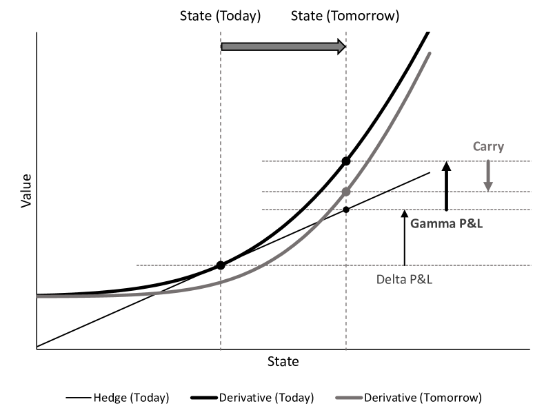
Figure 2: Over a time interval, the profit/loss that accrues on the derivative security is decomposed into the delta p&l, which is hedged using liquid underlying securities, the gamma p&l, the unhedgeable residual from the convexity of the price function, and carry, the appreciation over time. Fair pricing requires that accrual from gamma p&l is offset by carry.

Terms representing carry and gamma p&l are evident in the Black-Scholes equation for the price $\mathsf{c}[t,\mathsf{s}]$ of a derivative security contingent on the price $\mathsf{s}$ of an underlying security. In this model, the underlying price is assumed to diffuse lognormally. Dynamic hedging eliminates the market risk from the volatility of the underlying price; setting the funded return to zero then leads to the equation:

$$0=\frac{\partial\mathsf{c}}{\partial t}-r(\mathsf{c}-\mathsf{s}\frac{\partial\mathsf{c}}{\partial\mathsf{s}})+\frac{1}{2}\sigma^{2}\mathsf{s}^{2}\frac{\partial^{2}\mathsf{c}}{\partial\mathsf{s}^{2}}$$ (2)

for the derivative price, where $r$ is the funding rate and $\sigma$ is the lognormal volatility of the underlying price. The derivative is delta-hedged by an offsetting position in the underlying. Gamma p&l accrues for positive convexity when the underlying price is volatile, and the Black-Scholes equation balances this ‘volatility$\times$convexity’ accrual with the carry from time decay and the funding costs of the hedged position.

Generalisations of the Black-Scholes model have equivalent terms for these contributions, incorporating alternative volatility models for the underlying prices and other economic variables. The viability of this approach then depends on the effectiveness of the market risk transfer from derivative to underlying provided by dynamic hedging, and the accuracy of the model compared to realised market volatility over the lifetime of the derivative.

1 Economic principles for pricing

The elementary economic principles underpinning this argument are replicability and the absence of arbitrage, both essentially algebraic constraints on the valuation map from the observable that represents the settlement amount of the derivative to its price. As with all such principles, they are an approximation to the reality of financial markets, but their validity is assumed throughout the following.

The exposition rests on three founding economic principles:

The Principle of Replicability:

A security constructed as a linear combination of underlying securities has price equal to the same linear combination of underlying prices.

The Principle of No-Arbitrage:

A security that has positive settlement in all future scenarios has positive price.

The Principle of Economic Equivalence:

A security that has zero settlement in all possible future scenarios has zero price.

The first two principles are consistency conditions that disable the construction of arbitrages, and dictate that the valuation map is linear and positive. Prohibiting unattainable outcomes from impacting price, the final principle connects the valuation map with the forecasting model of the economy – expectations of future outcomes are not necessarily reflected in pricing, but this weaker requirement removes from consideration scenarios that have zero measure in the economic model, and so are deemed to be impossible. The connection between these economic principles and fundamental mathematical constructions is the main focus of this essay.

The principles of replicability and no-arbitrage connect price with the functional calculus of observables. Let $\mathsf{A}$ be the space of economic observables whose values can be ascertained at settlement. Following the opening comments, the payoff of the derivative in a nominated payment currency is represented as an observable in this space. The price model is then an operation:

$$\mathsf{z}:\mathsf{a}\in\mathsf{A}\mapsto\mathsf{z}\bullet\mathsf{a}\in\mathbb{R}$$ (3)

that maps the derivative payoff $\mathsf{a}$ to its price $\mathsf{z}\bullet\mathsf{a}$.

The principle of replicability imposes the homomorphic relationship with addition:

$$\mathsf{z}\bullet(\mathsf{a}+\mathsf{b})=(\mathsf{z}\bullet\mathsf{a})+(\mathsf{z}\bullet\mathsf{b})$$ (4)

thus ensuring that the price of a portfolio can be determined from the prices of its constituents. The principle of no-arbitrage does not impose the homomorphic relationship with multiplication, $\mathsf{z}\bullet(\mathsf{ab})=(\mathsf{z}\bullet\mathsf{a})(\mathsf{z}\bullet\mathsf{b})$, as this denies the possibility of extracting value from convexity, an essential property for a viable model of derivative prices. Instead, this principle imposes the weaker requirement that the price map is positive:

$$\mathsf{a}\geq 0\implies\mathsf{z}\bullet\mathsf{a}\geq 0$$ (5)

which in turn implies the sub-homomorphic relationship with multiplication:

$$(\mathsf{z}\bullet\mathsf{ab})^{2}\leq(\mathsf{z}\bullet\mathsf{a}^{2})(\mathsf{z}\bullet\mathsf{b}^{2})$$ (6)

This Cauchy-Schwarz inequality for the price model is satisfied by linear combinations of ring homomorphisms with positive weights.

The principle of economic equivalence connects price with the stochastic calculus of observables. The founding economic principles apply across any time interval $t_{i}\leq t_{j}$ with price model given by a linear and positive operation:

$$\mathsf{z}_{ij}:\mathsf{a}_{j}\in\mathsf{A}_{j}\mapsto\mathsf{z}_{ij}\bullet\mathsf{a}_{j}\in\mathsf{A}_{i}$$ (7)

that maps the derivative payoff $\mathsf{a}_{j}$ at time $t_{j}$ to its price $\mathsf{z}_{ij}\bullet\mathsf{a}_{j}$ at time $t_{i}$, where $\mathsf{A}_{i}\subset\mathsf{A}_{j}$ are the subspaces of observables whose values can be ascertained at the start and end of the interval.

The principle of economic equivalence relates these operations to the model of the economy:

$$\mathsf{z}_{ij}\bullet\mathsf{a}_{j}=\mathsf{\bar{z}}_{ij}\bullet\mathsf{w}_{ij}\mathsf{a}_{j}$$ (8)

where:

$$\mathsf{\bar{z}}_{ij}:\mathsf{a}_{j}\in\mathsf{A}_{j}\mapsto\mathsf{\bar{z}}_{ij}\bullet\mathsf{a}_{j}\in\mathsf{A}_{i}$$ (9)

is the expectation of observables at time $t_{j}$ conditional on observables at time $t_{i}$. The strictly-positive state-price deflator $\mathsf{w}_{ij}$ in this expression rescales the measure of an event in the economic model to the Arrow-Debreu price of the corresponding digital option. Consistency among the family of price operations requires that their compositions satisfy the tower law, a property that follows when the state-price deflators take the form $\mathsf{w}_{ij}=\mathsf{w}_{i}/\mathsf{w}_{j}$ for a strictly-positive numeraire process $\mathsf{w}$. The process $\mathsf{a}$ is then the price of a tradable security if it satisfies:

$$\frac{\mathsf{a}_{i}}{\mathsf{w}_{i}}=\mathsf{\bar{z}}_{ij}\bullet\frac{\mathsf{a}_{j}}{\mathsf{w}_{j}}$$ (10)

for each time interval $t_{i}\leq t_{j}$. The numeraire has the dimension of currency, so that the ratio of price over numeraire is dimensionless, and the price model states that this ratio is a martingale in the economic measure.

The price model decomposes into two components: the specification of an economic model that quantifies the conditional expectations of economic observables; and the identification of a numeraire process that adjusts these expectations to match underlying prices. The price model is not uniquely determined by the founding economic principles, and further principles are needed to explain the origin of the numeraire. Completion of the model requires an understanding of the roles that funding and hedging play in the optimisation of trading activity, leading to additional guidelines that crystallise the price of the derivative.

2 Funding

The economic principles govern pricing for all market participants, but do not fully determine price. Flexibility in the framework, exemplified by the unidentified numeraire $\mathsf{w}$, is only resolved by looking more closely at the activities within the financial institution.

Trading activity is funded by issuing bonds and shares, and the costs of this operation are charged to the desk via the strictly-positive unsecured funding price $\mathsf{u}$ representing the unit price of funding for the institution. Benchmarking against the cost of funding allows settlements at different times to be compared on a consistent basis, and this makes the unsecured funding price the natural candidate for numeraire in the price model. This hypothesis is overly restrictive, however, as there is no facility in the approach to mark the model to market. The contribution of funding to price is instead revealed by inspecting the funding settlements alongside those from the traded security in the context of the price model.

Consider the purchase at time $t$ for price $\mathsf{a}$ and the subsequent sale at time $t+dt$ for price $\mathsf{a}+d\mathsf{a}$ of a tradable security transacted over the finite time increment $dt$. The price model relates these initial and terminal prices via the local martingale condition:

$$0=\mathsf{\bar{z}}\bullet d\frac{\mathsf{a}}{\mathsf{w}}$$ (11)

for the conditional expectation from time $t+dt$ to time $t$ of the dimensionless ratio $\mathsf{a}/\mathsf{w}$. The purchase of the security is funded with the sale of $\mathsf{a}/\mathsf{u}$ units of unsecured funding, returning at time $t+dt$ the proceeds $\mathsf{a}+d\mathsf{a}$ from the resale of the security minus the costs $(\mathsf{a}/\mathsf{u})(\mathsf{u}+d\mathsf{u})$ from the repurchase of unsecured funding. Feeding these settlements into the price model leads to the alternative local martingale condition:

$$0=\mathsf{\bar{z}}\bullet\frac{d\mathsf{a}-(\mathsf{a}/\mathsf{u})\,d\mathsf{u}}{\mathsf{w}+d\mathsf{w}}=\mathsf{\bar{z}}\bullet\frac{\mathsf{u}+d\mathsf{u}}{\mathsf{w}+d\mathsf{w}}\,d\frac{\mathsf{a}}{\mathsf{u}}$$ (12)

From the perspective of the financial institution, there are now two representations of the local martingale condition for the same transaction. Fortunately, these conditions are aligned when the dimensionless ratio $\mathsf{u}/\mathsf{w}$ is a martingale:

$$0=\mathsf{\bar{z}}\bullet d\frac{\mathsf{u}}{\mathsf{w}}$$ (13)

The funding of trading activity thus imposes a normalisation constraint on the model: the numeraire does not necessarily equal the unsecured funding price, but their ratio is required to be driftless in the economic measure.

Recognising the elevated status of the unsecured funding price, the price measure $\mathsf{\hat{z}}$ is defined to be the measure equivalent to the economic measure $\mathsf{\bar{z}}$ with Radon-Nikodym kernel given by the martingale $\mathsf{u}/\mathsf{w}$. The price model is expressed in terms of this measure by the local martingale condition:

$$0=\mathsf{\hat{z}}\bullet\frac{d\mathsf{a}-(\mathsf{a}/\mathsf{u})\,d\mathsf{u}}{\mathsf{u}+d\mathsf{u}}=\mathsf{\hat{z}}\bullet d\frac{\mathsf{a}}{\mathsf{u}}$$ (14)

for the price $\mathsf{a}$ of a tradable security. In this form, the unsecured funding price $\mathsf{u}$ replaces the numeraire $\mathsf{w}$ as discounting for the security. Further principles are then needed to identify the price measure from the economic measure.

In addition to prescribing settlements, the derivative contract may also stipulate terms for its funding. Defining the price of the derivative as the discounted expectation in the price measure of its terminal settlements neglects these incremental funding settlements. More accurately, the derivative should be accounted for continuously, including any margin or collateral payments, or any other costs incurred by the use of financial resources.

The crucial consideration is the incremental settlement implied by the terms of the contract, and in this there is commonality across different derivative types. In each case, the derivative is associated with a market price $\mathsf{a}$ and a strictly-positive funding price $\mathsf{b}$ used to determine the net profit/loss over the time increment $dt$ for the self-funded position:

$$d\mathsf{a}-\frac{\mathsf{a}}{\mathsf{b}}d\mathsf{b}=(\mathsf{b}+d\mathsf{b})\,d\frac{\mathsf{a}}{\mathsf{b}}$$ (15)

This expression, which includes funding costs but neglects additional charges for reserves against potential unwind costs, comprises the profit/loss from derivative minus the profit/loss from funding, and the owner receives these net settlements for as long as they hold the derivative. Price is thus derived from the terminal settlements and binding provisions for funding as specified in the contract, varying according to the nature of the derivative.

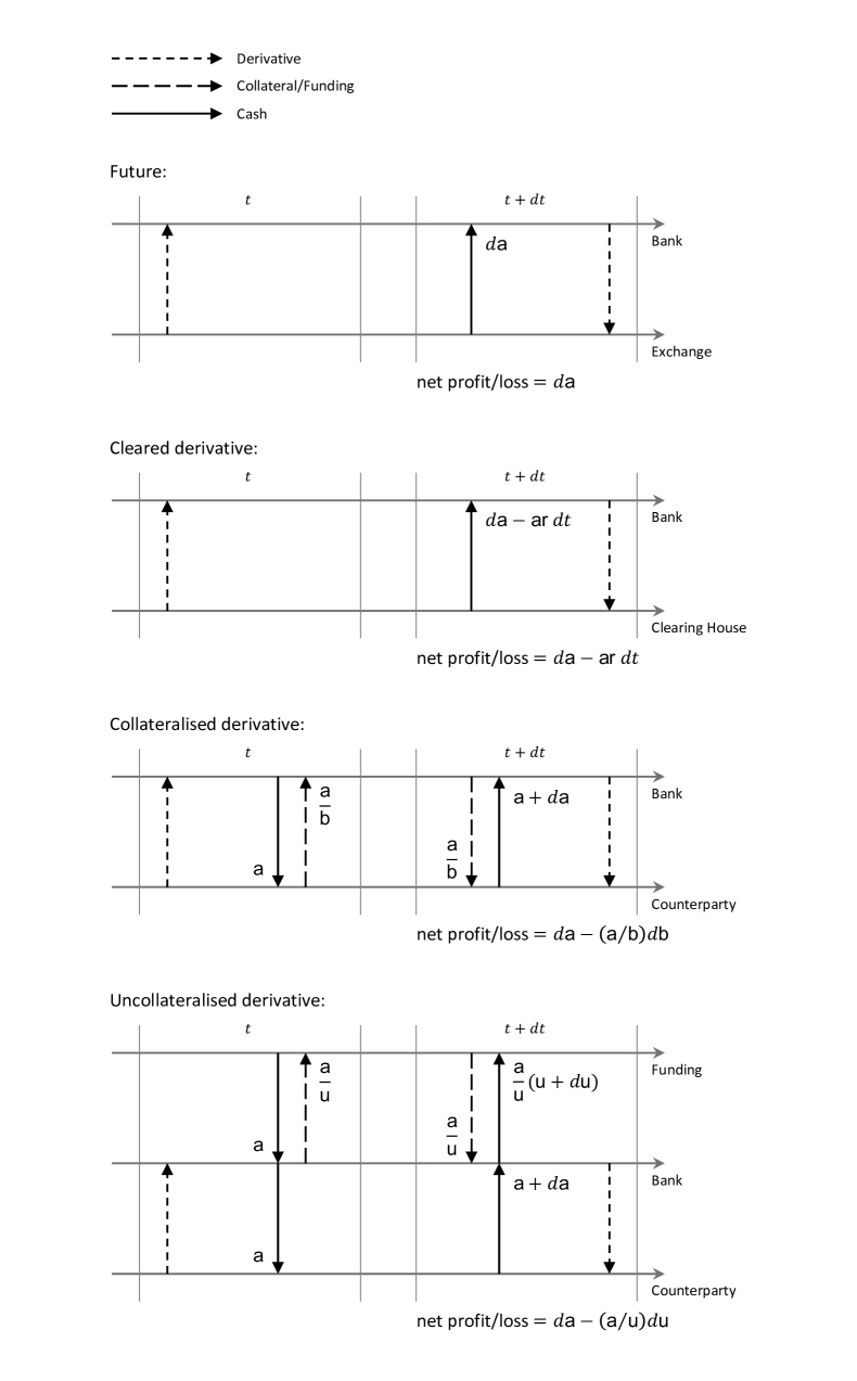
Figure 3: The execution and settlement exchanges associated with four types of derivative. Common to all these is the expression for the net profit/loss over the time interval, equal to the price change minus the cost of funding as prescribed by the derivative contract.

Futures

are standardised derivatives traded on exchanges, typically with high liquidity and low transaction costs. Participants use limit and market orders to submit prices and execute trades, thereafter committing the holder to the series of payments required to maintain the margin account. The net settlement over the time increment is the variation margin:

$$d\mathsf{a}$$ (16)

on the market price $\mathsf{a}$ of the future. In the general expression, this is equivalent to funding with the unit $\mathsf{b}=1$.

Cleared derivatives

extend the essential features of futures to a wider range of standardised derivatives. Market makers provide firm prices, and execution is intermediated by a clearing house whose exposure to default risk is mitigated through the maintenance of an interest-bearing margin account. The market price $\mathsf{a}$ serves as the reference for the variation margin settlement:

$$d\mathsf{a}-\mathsf{ar}\,dt$$ (17)

equivalent to funding with the cash account $\mathsf{b}=(1+\mathsf{r}\,dt)^{t/dt}$ that accrues interest at the rate $\mathsf{r}$ specified by the clearing house.

Collateralised derivatives

are bilateral transactions commonly used for more illiquid structures. Default risk is mitigated through the provision of collateral, whose terms are dictated by the legal relationship between the two parties. Collateral is continuously rebalanced to ensure it covers the derivative valuation. The net settlement over the time increment is then:

$$d\mathsf{a}-\frac{\mathsf{a}}{\mathsf{b}}d\mathsf{b}$$ (18)

being the variation of the derivative valuation $\mathsf{a}$ and the collateral valuation $\mathsf{b}$ in the collateral account.

Uncollateralised derivatives

offer bespoke derivative features to clients without requiring the exchange of collateral. The cost of unsecured funding, covering the anticipated closing price of the derivative, is charged back to the desk. The net settlement in the trading book is:

$$d\mathsf{a}-\frac{\mathsf{a}}{\mathsf{u}}d\mathsf{u}$$ (19)

netting the variation on the derivative valuation $\mathsf{a}$ and the incremental maintenance cost for unsecured funding with price $\mathsf{u}$.

For each of these types, holding the derivative becomes a commitment to a series of self-funded net settlements in the trading book, entered at zero cost and returning an amount that nets the variations on the market and funding valuations for the derivative. Inserting these initial and terminal prices into the price model leads to the local martingale condition:

$$0=\mathsf{\hat{z}}\bullet\frac{d\mathsf{a}-(\mathsf{a}/\mathsf{b})\,d\mathsf{b}}{\mathsf{u}+d\mathsf{u}}=\mathsf{\hat{z}}\bullet\frac{\mathsf{b}+d\mathsf{b}}{\mathsf{u}+d\mathsf{u}}\,d\frac{\mathsf{a}}{\mathsf{b}}$$ (20)

for the conditional expectation from time $t+dt$ to time $t$ of the dimensionless price ratio $\mathsf{a}/\mathsf{b}$. Margin settlements are made at the endpoints of each interval in a series $t_{0}<\cdots<t_{n}$ of times, and the local condition above is compounded to the martingale condition:

$$\frac{\mathsf{a}_{i}}{\mathsf{b}_{i}}=\mathsf{\hat{z}}_{ij}\bullet\prod_{k=i}^{j-1}\frac{\mathsf{b}_{k+1}/\mathsf{u}_{k+1}}{\mathsf{\hat{z}}_{k\,k+1}\bullet\mathsf{b}_{k+1}/\mathsf{u}_{k+1}}\frac{\mathsf{a}_{j}}{\mathsf{b}_{j}}$$ (21)

The role of numeraire in this expression is taken by the funding price, and the ratio of market price over funding price is a martingale in a measure associated with the funding that is equivalent to the price measure.

Utilising the funding price as numeraire resolves the discounting question for the settlements of the derivative. The correction to the price measure is required to ensure consistency across the models generated for different funding arrangements. In each case, the change of measure is driven by the convexity between the funding price $\mathsf{b}$ of the derivative and the unsecured funding price $\mathsf{u}$ of the financial institution, with Radon-Nikodym kernel given by the dimensionless funding ratio $\mathsf{b}/\mathsf{u}$ drift-adjusted to be a martingale in the price measure.

A natural hierarchy exists in the market, with futures and cleared derivatives providing the price transparency and liquidity to mark-to-market bilateral derivatives. This market information is absorbed in the price model through the mechanism of hedging, with the price measure emerging from a martingale condition derived from fair pricing principles.

3 Hedging

Bridging the gap between the subjective expectations encapsulated in the model for the economy and the market expectations expressed by the prices of liquid securities is not without ambiguity, but guidance can be found in traditional methods of portfolio optimisation. In the following, this ambiguity is resolved by removing bias in optimal strategies based on the mean and variance of portfolio returns, exploiting the market stratification into liquid underlying securities used for hedging and derivative securities marked-to-market following fair pricing principles.

The performance of the strategy is measured relative to the unsecured funding price $\mathsf{u}$ of the financial institution using the statistics from the economic model $\mathsf{\bar{z}}$. For the strategy with price $\mathsf{a}$, performance is quantified by the mean and variance of the increment $d(\mathsf{a}/\mathsf{u})$, delimiting the expected range for the return on the strategy in proportion to the reference price. Benchmarking against unsecured funding removes the dependency on the denominating currency and allows the consistent evaluation of settlements at different times.

While this is an effective method for combining economic and market expectations in the price model, it is not necessarily an accurate representation of risk management activities in a financial institution. Both the economic model and the unsecured funding price depend on the institution, and the resulting price model is sensitive to these components. Furthermore, using mean and variance as targets for optimisation may not be suited to the management of extreme events, and alternative statistics will lead to variations in the derivative price. For these reasons, the principle of portfolio optimisation that completes the price model is here held separate from the three core economic principles.

3.1 Portfolio optimisation

The market provides access to a set of liquid underlying securities whose vectors of market prices $\mathsf{p}$ and funding prices $\mathsf{q}$ are directly observed. Normalised using the unsecured funding price $\mathsf{u}$, the return from the underlying securities over the trading interval is:

$$\mathsf{R}_{\mathsf{p}}=\frac{d\mathsf{p}-(\mathsf{p}/\mathsf{q})\,d\mathsf{q}}{\mathsf{u}+d\mathsf{u}}=\frac{\mathsf{q}+d\mathsf{q}}{\mathsf{u}+d\mathsf{u}}\,d\frac{\mathsf{p}}{\mathsf{q}}$$ (22)

The return is adjusted to account for the convexity between underlying and unsecured funding, captured in the dimensionless funding ratio $\mathsf{q}/\mathsf{u}$. The anticipated range for the return vector $\mathsf{R}_{\mathsf{p}}$ is quantified in terms of the mean vector $\mathsf{M}_{\mathsf{p}}$ and covariance matrix $\mathsf{V}_{\mathsf{p}}$:

$$\mathsf{M}_{\mathsf{p}} =\mathsf{\bar{z}}\bullet\mathsf{R}_{\mathsf{p}}$$ (23)

$$\mathsf{V}_{\mathsf{p}} =\mathsf{\bar{z}}\bullet\mathsf{R}_{\mathsf{p}}^{2}-(\mathsf{\bar{z}}\bullet\mathsf{R}_{\mathsf{p}})^{2}$$

The effectiveness of the investment strategy then depends on its success in identifying portfolios that minimise risk for a target expected return.

The expected performance of the underlying portfolio is measured by the mean $\mathsf{m}=\alpha\cdot\mathsf{M}_{\mathsf{p}}$ and variance $\mathsf{v}=\alpha\cdot\mathsf{V}_{\mathsf{p}}\alpha$ of its return, where the composition of the portfolio is specified by the weights $\alpha$. The economic model considers the return on portfolios with zero variance to be guaranteed, and unless the mean is also zero this implies the existence of an arbitrage. The technical requirement for the economic model to avoid arbitrage is:

$$\ker[\mathsf{V}_{\mathsf{p}}]\cdot\mathsf{M}_{\mathsf{p}}=\{0\}$$ (24)

For convenience, the stronger condition $\ker[\mathsf{V}_{\mathsf{p}}]=\{0\}$ is assumed in the following. In the more general case, the optimal strategies developed here are valid only when the economic model satisfies the no-arbitrage constraint, and are then determined only up to the addition of a zero-variance portfolio.

Optimal portfolio weights, achieving the minimum possible variance for a target mean, satisfy the stationarity condition:

$$0 =\delta(\alpha\cdot\mathsf{V}_{\mathsf{p}}\alpha+\lambda(\alpha\cdot\mathsf{M}_{\mathsf{p}}-\mathsf{m}))$$ (25)

$$=\delta\alpha\cdot(2\mathsf{V}_{\mathsf{p}}\alpha+\lambda\mathsf{M}_{\mathsf{p}})$$

under variations $\delta\alpha$ of the portfolio $\alpha$, where the Lagrange multiplier $\lambda$ maps to the risk appetite of the investor. The optimal portfolio is thus:

$$\alpha\propto\mathsf{V}_{\mathsf{p}}^{-1}\mathsf{M}_{\mathsf{p}}$$ (26)

The mean and variance achieved by this strategy lie on the parabola specified by the relation:

$$\frac{\mathsf{m}}{\sqrt{\mathsf{v}}}=\sqrt{\mathsf{V}_{\mathsf{p}}^{-1}\mathsf{M}_{\mathsf{p}}\cdot\mathsf{M}_{\mathsf{p}}}$$ (27)

where the expression on the right quantifies market sentiment on the expected return that is acceptable for a unit of risk. The optimal investment strategy minimises variance by diversifying risks across the underlying securities, with the risk appetite determining the position of the strategy on the efficient frontier parabola in mean-variance space.

3.2 Derivative pricing

Now consider a stratified market comprising the underlying securities with market prices $\mathsf{p}$ and funding prices $\mathsf{q}$ and a derivative security with market price $\mathsf{a}$ and funding price $\mathsf{b}$. The underlying securities constitute the hedge market for the derivative security, with the observed prices of the former used to mark-to-market the latter via fair pricing principles.

The strategy is optimised against the joint moments of the underlying return $\mathsf{R}_{\mathsf{p}}$ and the normalised return $\mathsf{R}_{\mathsf{a}}$ on the derivative:

$$\mathsf{R}_{\mathsf{a}}=\frac{d\mathsf{a}-(\mathsf{a}/\mathsf{b})\,d\mathsf{b}}{\mathsf{u}+d\mathsf{u}}=\frac{\mathsf{b}+d\mathsf{b}}{\mathsf{u}+d\mathsf{u}}\,d\frac{\mathsf{a}}{\mathsf{b}}$$ (28)

In addition to the mean vector $\mathsf{M}_{\mathsf{p}}$ and covariance matrix $\mathsf{V}_{\mathsf{p}}$ for the underlyings, the performance of the combined portfolio is quantified in terms of the mean $\mathsf{M}_{\mathsf{a}}$ and variance $\mathsf{V}_{\mathsf{a}}$ for the derivative:

$$\mathsf{M}_{\mathsf{a}} =\mathsf{\bar{z}}\bullet\mathsf{R}_{\mathsf{a}}$$ (29)

$$\mathsf{V}_{\mathsf{a}} =\mathsf{\bar{z}}\bullet\mathsf{R}_{\mathsf{a}}^{2}-(\mathsf{\bar{z}}\bullet\mathsf{R}_{\mathsf{a}})^{2}$$

and the cross-covariance vector $\mathsf{C}_{\mathsf{pa}}$:

$$\mathsf{C}_{\mathsf{pa}}=\mathsf{\bar{z}}\bullet\mathsf{R}_{\mathsf{p}}\mathsf{R}_{\mathsf{a}}-(\mathsf{\bar{z}}\bullet\mathsf{R}_{\mathsf{p}})(\mathsf{\bar{z}}\bullet\mathsf{R}_{\mathsf{a}})$$ (30)

Strategies for optimising the hedged derivative portfolio are determined from these statistics.

The introduction of the derivative expands the opportunities for diversification, leading to an incremental improvement in the expected return for a unit of risk from the optimal strategy:

$$\begin{bmatrix}\mathsf{V}_{\mathsf{p}}&\mathsf{C}_{\mathsf{pa}}\\ \mathsf{C}_{\mathsf{pa}}^{t}&\mathsf{V}_{\mathsf{a}}\end{bmatrix}^{-1}\begin{bmatrix}\mathsf{M}_{\mathsf{p}}\\ \mathsf{M}_{\mathsf{a}}\end{bmatrix}\cdot\begin{bmatrix}\mathsf{M}_{\mathsf{p}}\\ \mathsf{M}_{\mathsf{a}}\end{bmatrix}=\mathsf{V}_{\mathsf{p}}^{-1}\mathsf{M}_{\mathsf{p}}\cdot\mathsf{M}_{\mathsf{p}}+\frac{(\mathsf{M}_{\mathsf{a}}-\mathsf{V}_{\mathsf{p}}^{-1}\mathsf{M}_{\mathsf{p}}\cdot\mathsf{C}_{\mathsf{pa}})^{2}}{\mathsf{V}_{\mathsf{a}}-\mathsf{V}_{\mathsf{p}}^{-1}\mathsf{C}_{\mathsf{pa}}\cdot\mathsf{C}_{\mathsf{pa}}}$$ (31)

Activity in the underlying market uncovers the performance target of participants, and this suggests a principle for marking-to-market the fair price of the derivative.

The Principle of Portfolio Optimisation:

The derivative security does not increase the expected return for a unit of risk.

As can be seen from the expression above, this principle leads to the following condition for the fair price of the derivative:

$$\mathsf{M}_{\mathsf{a}}=\mathsf{V}_{\mathsf{p}}^{-1}\mathsf{M}_{\mathsf{p}}\cdot\mathsf{C}_{\mathsf{pa}}$$ (32)

Any other price for the derivative could be exploited in a strategy that out-performs the underlying market, and so market efficiency drives the price toward this equilibrium.

An alternative approach looks directly at the optimal portfolio that hedges the derivative return. For hedge weights $\beta$, the return on the hedged derivative has mean $\mathsf{m}$ and variance $\mathsf{v}$ given by:

$$\mathsf{m} =\mathsf{M}_{\mathsf{a}}-\beta\cdot\mathsf{M}_{\mathsf{p}}$$ (33)

$$\mathsf{v} =\mathsf{V}_{\mathsf{a}}-2\beta\cdot\mathsf{C}_{\mathsf{pa}}+\beta\cdot\mathsf{V}_{\mathsf{p}}\beta$$

The optimal hedge weights, achieving the minimum possible variance, then satisfy the stationarity condition:

$$0 =\delta(\mathsf{V}_{\mathsf{a}}-2\beta\cdot\mathsf{C}_{\mathsf{pa}}+\beta\cdot\mathsf{V}_{\mathsf{p}}\beta)$$ (34)

$$=2\delta\beta\cdot(\mathsf{V}_{\mathsf{p}}\beta-\mathsf{C}_{\mathsf{pa}})$$

under variations $\delta\beta$ of the portfolio $\beta$. The hedge portfolio is thus:

$$\beta=\mathsf{V}_{\mathsf{p}}^{-1}\mathsf{C}_{\mathsf{pa}}$$ (35)

The mean and variance achieved by this strategy are:

$$\mathsf{m} =\mathsf{M}_{\mathsf{a}}-\mathsf{V}_{\mathsf{p}}^{-1}\mathsf{M}_{\mathsf{p}}\cdot\mathsf{C}_{\mathsf{pa}}$$ (36)

$$\mathsf{v} =\mathsf{V}_{\mathsf{a}}-\mathsf{V}_{\mathsf{p}}^{-1}\mathsf{C}_{\mathsf{pa}}\cdot\mathsf{C}_{\mathsf{pa}}$$

The hedge does not eliminate the market risk of the derivative, but this strategy reduces it to the minimum achievable. This suggests an alternative principle for determining the fair price of the derivative.

The Principle of Portfolio Optimisation:

The return on a hedged derivative security is unbiased.

The implied expression for the fair price of the derivative is then:

$$\mathsf{M}_{\mathsf{a}}=\mathsf{V}_{\mathsf{p}}^{-1}\mathsf{M}_{\mathsf{p}}\cdot\mathsf{C}_{\mathsf{pa}}$$ (37)

The efficient market equilibrates at the level that removes bias in the residual hedged return, thereby calibrating the derivative price to the market. Conveniently, both principles for marking-to-market the derivative lead to the same fair pricing expression.

Market completeness – the capacity of the market to replicate the sensitivities of the derivative price – impacts the residual variance of the hedged derivative. Consider the underlying market with two sectors whose returns are $\mathsf{R}_{\mathsf{p}}$ and $\mathsf{R}_{\mathsf{o}}$ respectively. The optimal hedge in this case comprises a portfolio $\beta_{\mathsf{p}}$ in the first sector and a portfolio $\beta_{\mathsf{o}}$ in the second sector:

$$\begin{bmatrix}\beta_{\mathsf{p}}\\ \beta_{\mathsf{o}}\end{bmatrix}=\, \begin{bmatrix}\mathsf{V}_{\mathsf{p}}^{-1}\mathsf{C}_{\mathsf{pa}}\\ 0\end{bmatrix}$$ (38)

$$+\begin{bmatrix}-\mathsf{V}_{\mathsf{p}}^{-1}\mathsf{C}_{\mathsf{po}}(\mathsf{V}_{\mathsf{o}}-\mathsf{C}_{\mathsf{po}}^{t}\mathsf{V}_{\mathsf{p}}^{-1}\mathsf{C}_{\mathsf{po}})^{-1}(\mathsf{C}_{\mathsf{oa}}-\mathsf{C}_{\mathsf{po}}^{t}\mathsf{V}_{\mathsf{p}}^{-1}\mathsf{C}_{\mathsf{pa}})\\ (\mathsf{V}_{\mathsf{o}}-\mathsf{C}_{\mathsf{po}}^{t}\mathsf{V}_{\mathsf{p}}^{-1}\mathsf{C}_{\mathsf{po}})^{-1}(\mathsf{C}_{\mathsf{oa}}-\mathsf{C}_{\mathsf{po}}^{t}\mathsf{V}_{\mathsf{p}}^{-1}\mathsf{C}_{\mathsf{pa}})\end{bmatrix}$$

The first term on the right is the optimal strategy when only the first sector is available for hedging. The second term improves hedge performance by substituting part of the first sector hedge with securities from the second sector that better replicate the return on the derivative. This leads to an incremental reduction in the variance of the hedged derivative:

$$\mathsf{v}=\, \mathsf{V}_{\mathsf{a}}-\mathsf{V}_{\mathsf{p}}^{-1}\mathsf{C}_{\mathsf{pa}}\cdot\mathsf{C}_{\mathsf{pa}}$$ (39)

$$-(\mathsf{V}_{\mathsf{o}}-\mathsf{C}_{\mathsf{po}}^{t}\mathsf{V}_{\mathsf{p}}^{-1}\mathsf{C}_{\mathsf{po}})^{-1}(\mathsf{C}_{\mathsf{oa}}-\mathsf{C}_{\mathsf{po}}^{t}\mathsf{V}_{\mathsf{p}}^{-1}\mathsf{C}_{\mathsf{pa}})\cdot(\mathsf{C}_{\mathsf{oa}}-\mathsf{C}_{\mathsf{po}}^{t}\mathsf{V}_{\mathsf{p}}^{-1}\mathsf{C}_{\mathsf{pa}})$$

Each expansion in the range of hedge securities enhances the opportunities for offsetting the risk of the derivative.

By setting the expected return on the hedged derivative to zero, the price model interpolates between two accounting methodologies. At one extreme, when the underlying market is empty price is identified with expectation. At the opposite extreme, when the underlying market is complete price is determined by replication. The extent to which the price model relies on expectation versus replication depends on market completeness: the sensitivity of price to the economic model is mitigated by the calibration to available market prices; conversely, the economic model plugs the gap in pricing when liquidity is limited.

3.3 Hedge performance

For the observables within a time interval, the economic model provides two measures: the forecast measure and the empirical measure.

Forecast measure:

The measure $\mathsf{\bar{z}}^{s}$ seen at the start of the time interval, capturing the predicted statistics for the observables.

Empirical measure:

The measure $\mathsf{\bar{z}}^{e}$ seen at the end of the time interval, capturing the observed statistics for the observables.

Construction of the economic model begins with a reduction to the macroscopic variables that describe the economy, and proceeds with the consistent assignment of probabilities for the values of these observables. Evidence refines these assignments: the measure starts as informed guess and ends as statistical analysis. Performance of the economic model is then quantified by the gap between its forecast and empirical measures.

These measures respectively generate the hedge strategies:

$$\beta^{s} =\mathsf{V}_{\mathsf{p}}^{s}{}^{-1}\mathsf{C}_{\mathsf{pa}}^{s}$$ (40)

$$\beta^{e} =\mathsf{V}_{\mathsf{p}}^{e}{}^{-1}\mathsf{C}_{\mathsf{pa}}^{e}$$

The first portfolio is the optimal strategy computed at the start of the interval, based on initial expectations for the future of the economy. The second portfolio is the optimal strategy computed at the end of the interval, hedging with the benefit of hindsight according to the realised market volatility over the interval.

The executed hedge strategy is necessarily derived from the forecast measure. Hedge performance is then quantified by the empirical mean $\mathsf{m}$ and variance $\mathsf{v}$ of the return on the hedged derivative:

$$\mathsf{m} =(\mathsf{M}_{\mathsf{a}}^{e}-\mathsf{V}_{\mathsf{p}}^{e}{}^{-1}\mathsf{M}_{\mathsf{p}}^{e}\cdot\mathsf{C}_{\mathsf{pa}}^{e})+(\beta^{e}-\beta^{s})\cdot\mathsf{M}_{\mathsf{p}}^{e}$$ (41)

$$\mathsf{v} =(\mathsf{V}_{\mathsf{a}}^{e}-\mathsf{V}_{\mathsf{p}}^{e}{}^{-1}\mathsf{C}_{\mathsf{pa}}^{e}\cdot\mathsf{C}_{\mathsf{pa}}^{e})+(\beta^{e}-\beta^{s})\cdot\mathsf{V}_{\mathsf{p}}^{e}(\beta^{e}-\beta^{s})$$

The empirical variance decomposes into two components. The market risk component is the minimum variance achievable in the empirical measure using the empirical hedge strategy. The model risk component is the additional variance due to the sub-optimality of the forecast hedge strategy.

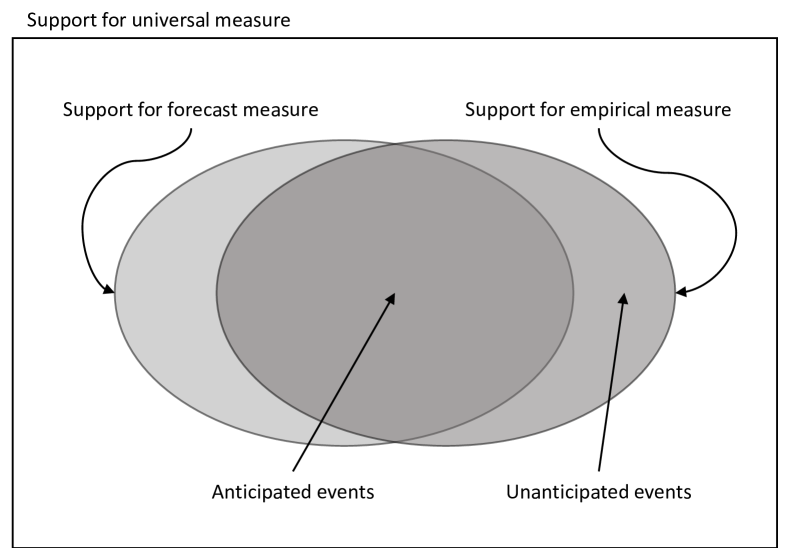
Figure 4: The support for the empirical measure divides into the anticipated events shared with the forecast measure and the unanticipated events with zero forecast measure.

The forecast and empirical measures are not necessarily equivalent: events that are anticipated may not materialise; conversely, and more dangerously, unanticipated ‘black swan’ events accounted in the empirical measure are neglected in the forecast measure. Introduce a universal measure $\mathsf{z}$ that supports the events for both measures, with Radon-Nikodym kernels expressed as:

$$\frac{d\mathsf{\bar{z}}^{s}}{d\mathsf{z}} =\mathsf{A}$$ (42)

$$\frac{d\mathsf{\bar{z}}^{e}}{d\mathsf{z}} =\mathsf{A}+\varepsilon\mathsf{D}$$

The empirical measure corrects the forecast measure via the term $\varepsilon\mathsf{D}$. Considering the case when $\varepsilon$ is small, the difference between the empirical and forecast hedges is expanded:

$$\beta^{e}-\beta^{s}=\mathsf{V}_{\mathsf{p}}^{s}{}^{-1}\Omega+O[\varepsilon^{2}]$$ (43)

where:

$$\Omega=\mathsf{z}\bullet\varepsilon\mathsf{D}(\mathsf{R}_{\mathsf{p}}-\mathsf{\bar{z}}^{s}\bullet\mathsf{R}_{\mathsf{p}})(\mathsf{R}_{\mathsf{a}}-\beta^{s}\cdot\mathsf{R}_{\mathsf{p}})$$ (44)

Sub-optimality of the forecast hedge is proportional to the deviation of the empirical measure from the forecast measure. It is also proportional to the residual return from the hedged derivative, confirming that market completeness is a determinant for the performance of the hedge.

Anticipated and unanticipated events are separated in the correction term:

$$\mathsf{D}=\mathsf{SA}+\mathsf{B}$$ (45)

where $\mathsf{B}$ satisfies $\mathsf{AB}=0$. Relative to the universal measure, the empirical measure deviates from the forecast measure by the kernel $\varepsilon(\mathsf{SA}+\mathsf{B})$ where $\varepsilon\mathsf{SA}$ corrects the measure for anticipated events and $\varepsilon\mathsf{B}$ appends the measure for unanticipated events. The expression for the hedge error decomposes as:

$$\Omega=\Omega_{a}+\Omega_{b}$$ (46)

The first term in the decomposition:

$$\Omega_{a}=\mathsf{\bar{z}}^{s}\bullet\varepsilon\mathsf{S}(\mathsf{R}_{\mathsf{p}}-\mathsf{\bar{z}}^{s}\bullet\mathsf{R}_{\mathsf{p}})(\mathsf{R}_{\mathsf{a}}-\beta^{s}\cdot\mathsf{R}_{\mathsf{p}})$$ (47)

is the hedge error arising from the adjustment $\mathsf{S}$ that rescales the probabilities of anticipated events following the assessment of actual market volatility over the interval. The second term in the decomposition:

$$\Omega_{b}=\mathsf{\bar{z}}^{e}\bullet(\mathsf{B}\neq 0)(\mathsf{R}_{\mathsf{p}}-\mathsf{\bar{z}}^{s}\bullet\mathsf{R}_{\mathsf{p}})(\mathsf{R}_{\mathsf{a}}-\beta^{s}\cdot\mathsf{R}_{\mathsf{p}})$$ (48)

is the hedge error arising from the unanticipated events indicated by the condition $\mathsf{B}\neq 0$. The first term, the ‘known-unknown’ contribution to model risk, is evaluated within the context of the forecast measure by estimating the error bounds for model parameters. The second term, the ‘unknown-unknown’ contribution to model risk, is harder to assess in advance as it is measured against events that are initially assumed to be impossible.

4 Expectation and price

The founding economic principles dictate that the incremental change in the price ratio of the derivative security satisfies the local martingale condition:

$$0=\mathsf{\hat{z}}\bullet\frac{\mathsf{b}+d\mathsf{b}}{\mathsf{u}+d\mathsf{u}}\,d\frac{\mathsf{a}}{\mathsf{b}}$$ (49)

where the price measure $\mathsf{\hat{z}}$ adjusts the economic measure $\mathsf{\bar{z}}$, calibrating to the underlying securities via the local martingale condition:

$$0=\mathsf{\hat{z}}\bullet\frac{\mathsf{q}+d\mathsf{q}}{\mathsf{u}+d\mathsf{u}}\,d\frac{\mathsf{p}}{\mathsf{q}}$$ (50)

for the incremental changes in the price ratios of the underlying securities. This price model satisfies the principles of replication and economic equivalence by construction; it satisfies the principle of no-arbitrage when the price measure is positive.

While the role of economic expectation in price determination is clear from these local martingale conditions, the economic principles and market calibrations do not uniquely determine the price measure. Taking its steer from portfolio optimisation, the previous section derives an additional condition for the fair price of the derivative by removing bias in the return from the hedged portfolio. This resolves the ambiguity in the price model.

Expanding the terms in the fair pricing condition that include the return on the derivative security leads to:

$$\mathsf{\bar{z}}\bullet\mathsf{R}_{\mathsf{a}}=\mathsf{\bar{z}}\bullet\mathsf{V}_{\mathsf{p}}^{-1}\mathsf{M}_{\mathsf{p}}\cdot(\mathsf{R}_{\mathsf{p}}-\mathsf{\bar{z}}\bullet\mathsf{R}_{\mathsf{p}})\mathsf{R}_{\mathsf{a}}$$ (51)

This is re-arranged to the following relation for the incremental change in the derivative price ratio:

$$0=\mathsf{\bar{z}}[\alpha]\bullet\frac{\mathsf{b}+d\mathsf{b}}{\mathsf{u}+d\mathsf{u}}\,d\frac{\mathsf{a}}{\mathsf{b}}$$ (52)

where the dimensionless parameters $\alpha$ are marked-to-market via the relation:

$$0=\mathsf{\bar{z}}[\alpha]\bullet\frac{\mathsf{q}+d\mathsf{q}}{\mathsf{u}+d\mathsf{u}}\,d\frac{\mathsf{p}}{\mathsf{q}}$$ (53)

for the incremental changes in the underlying price ratios. The price measure $\mathsf{\hat{z}}=\mathsf{\bar{z}}[\alpha]$ in these expressions is equivalent to the economic measure $\mathsf{\bar{z}}$, with Radon-Nikodym kernel adjusting for the returns on the underlying securities:

$$\frac{d\mathsf{\bar{z}}[\alpha]}{d\mathsf{\bar{z}}}=1-\alpha\cdot(\frac{\mathsf{q}+d\mathsf{q}}{\mathsf{u}+d\mathsf{u}}\,d\frac{\mathsf{p}}{\mathsf{q}}-\mathsf{\bar{z}}\bullet\frac{\mathsf{q}+d\mathsf{q}}{\mathsf{u}+d\mathsf{u}}\,d\frac{\mathsf{p}}{\mathsf{q}})$$ (54)

In this representation, the funding price assumes the mantle of numeraire, and the economic measure is tweaked to calibrate the price measure to market prices. Direct comparison with the general expression confirms that this price model satisfies the principles of replication and economic equivalence. It does not, however, satisfy the principle of no-arbitrage: if the underlying price changes deviate significantly from their expectations, the kernel could be negative. This highlights the inadequacies of mean-variance optimisation as a method of price determination. By under-estimating the impact of tail events, these performance metrics leave open the possibility of arbitrage.

The defect in the price model is resolved by substituting the linear kernel with the following exponential alternative:

$$\frac{d\mathsf{\bar{z}}[\alpha]}{d\mathsf{\bar{z}}}=\frac{\exp\!\left[-\alpha\cdot\dfrac{\mathsf{q}+d\mathsf{q}}{\mathsf{u}+d\mathsf{u}}\,d\dfrac{\mathsf{p}}{\mathsf{q}}\right]}{\mathsf{\bar{z}}\bullet\exp\!\left[-\alpha\cdot\dfrac{\mathsf{q}+d\mathsf{q}}{\mathsf{u}+d\mathsf{u}}\,d\dfrac{\mathsf{p}}{\mathsf{q}}\right]}$$ (55)

This variant of the price model is justified as it converges to the original when the underlying return is small and avoids arbitrage when the underlying return is large, reweighting the performance measure to avoid arbitrage from tail events. The market calibration is solved by iterating the Newton-Raphson scheme:

$$\alpha\mapsto\alpha+\mathsf{V}_{\mathsf{p}}[\alpha]^{-1}\mathsf{M}_{\mathsf{p}}[\alpha]$$ (56)

where the mean vector $\mathsf{M}_{\mathsf{p}}[\alpha]$ and covariance matrix $\mathsf{V}_{\mathsf{p}}[\alpha]$ are computed using the equivalent measure $\mathsf{\bar{z}}[\alpha]$ from the preceding iteration. Starting with $\alpha=0$, convergence of this scheme then relies on the invertibility of the covariance at each iteration. Calibration determines a portfolio of underlying securities whose return is exponentiated to generate the kernel for the price measure relative to the economic measure, with weights $\alpha$ that control the deviation of the underlying prices from their expectations.

The price expression is compounded on the margin settlement schedule to generate the martingale condition for the derivative price ratio:

$$\frac{\mathsf{a}_{i}}{\mathsf{b}_{i}}=\mathsf{\bar{z}}_{ij}\bullet\prod_{k=i}^{j-1}\frac{\exp[-\alpha_{k}\cdot(\mathsf{q}_{k+1}/\mathsf{u}_{k+1})\,d(\mathsf{p}_{k}/\mathsf{q}_{k})]\,\mathsf{b}_{k+1}/\mathsf{u}_{k+1}}{\mathsf{\bar{z}}_{k\,k+1}\bullet\exp[-\alpha_{k}\cdot(\mathsf{q}_{k+1}/\mathsf{u}_{k+1})\,d(\mathsf{p}_{k}/\mathsf{q}_{k})]\,\mathsf{b}_{k+1}/\mathsf{u}_{k+1}}\frac{\mathsf{a}_{j}}{\mathsf{b}_{j}}$$ (57)

This expression determines the price of the derivative as the expectation of its discounted terminal settlement, where discounting matches funding and the measure is adjusted to calibrate underlying prices and accommodate convexity between the funding ratio and the returns on underlying securities.

  MAXIMUM ENTROPY PRICE MODEL The ingredients of the maximum entropy price model are the economic measure $\mathsf{\bar{z}}$ quantifying the expectations of economic observables, the unsecured funding price $\mathsf{u}$ of the financial institution, and the observed market prices $\mathsf{p}$ and funding prices $\mathsf{q}$ of liquid underlying securities. For a derivative security with market price $\mathsf{a}$ and funding price $\mathsf{b}$, the price model is given by the local martingale condition: $$0=\mathsf{\bar{z}}\bullet\exp\!\left[-\alpha\cdot\frac{\mathsf{q}+d\mathsf{q}}{\mathsf{u}+d\mathsf{u}}\,d\dfrac{\mathsf{p}}{\mathsf{q}}\right]\frac{\mathsf{b}+d\mathsf{b}}{\mathsf{u}+d\mathsf{u}}\,d\dfrac{\mathsf{a}}{\mathsf{b}}$$ for the change in the derivative price ratio $\mathsf{a}/\mathsf{b}$ over the time step $dt$, where the coefficients $\alpha$ mark the model to the underlying prices via the local martingale condition: $$0=\mathsf{\bar{z}}\bullet\exp\!\left[-\alpha\cdot\frac{\mathsf{q}+d\mathsf{q}}{\mathsf{u}+d\mathsf{u}}\,d\dfrac{\mathsf{p}}{\mathsf{q}}\right]\frac{\mathsf{q}+d\mathsf{q}}{\mathsf{u}+d\mathsf{u}}\,d\dfrac{\mathsf{p}}{\mathsf{q}}$$ for the change in the underlying price ratios $\mathsf{p}/\mathsf{q}$ over the time step $dt$. The price model assumes the expected return on the funded derivative, normalised by the unsecured funding price, is zero in the price measure that calibrates the economic measure to underlying prices with minimum relative entropy.

In a Bayesian interpretation of the approach, the economic measure is considered to be the maximum entropy state representing the best assumptions on price in the absence of market information. Assessed relative to this state, the price measure with exponential form for the kernel is the measure that maximises entropy while calibrating to the available prices of underlying securities. The price model, originally derived from the principles of no-arbitrage and portfolio optimisation, is then equivalently derived on the assumption of maximum entropy.

The Maximum Entropy Principle:

The price measure minimises entropy relative to the economic measure subject to calibration to the prices of liquid underlying securities.

Market intelligence on price is incomplete, and this principle proposes that the information vacuum is filled by the expectations quantified in the economic model. This is achieved by minimising the relative entropy of the price measure from the economic measure, subject to the mark-to-market constraints. The stationarity condition, whose solution is the exponential kernel $d\mathsf{\bar{z}}[\alpha]/d\mathsf{\bar{z}}$ defined above, is:

$$0 =\delta(\mathsf{\bar{z}}\bullet\mathsf{W}\log[\mathsf{W}]+\lambda(\mathsf{\bar{z}}\bullet\mathsf{W}-1)+\alpha\cdot\mathsf{\bar{z}}\bullet\mathsf{W}\frac{\mathsf{q}+d\mathsf{q}}{\mathsf{u}+d\mathsf{u}}\,d\frac{\mathsf{p}}{\mathsf{q}})$$ (58)

$$=\mathsf{\bar{z}}\bullet\delta\mathsf{W}(\log[\mathsf{W}]+(1+\lambda)+\alpha\cdot\frac{\mathsf{q}+d\mathsf{q}}{\mathsf{u}+d\mathsf{u}}\,d\frac{\mathsf{p}}{\mathsf{q}})$$

for variations $\delta\mathsf{W}$ of the kernel $\mathsf{W}$. The Lagrange multipliers $\lambda$ and $\alpha$ are solved for the normalisation constraint $\mathsf{\bar{z}}\bullet\mathsf{W}=1$ and the market calibrations.

Maximum entropy states arise in thermodynamic applications for the macroscopic variables of a system whose microscopic variables evolve on a much shorter timescale. In this perspective, the portfolio weights $\alpha$ are the inverse-temperatures for the underlying securities – ‘hot’ securities discover the equilibrium of the economic model, while ‘cold’ securities have prices that deviate from expectations. This analogy between non-equilibrium thermodynamics and economic agents discovering price through trading activity suggests an alternative route to the price model which will not be pursued further here.

5 Continuous settlement

The incremental price condition is compounded on the margin settlement schedule, and the ratio of market price over funding price for the derivative is a martingale on this schedule in an equivalent measure that calibrates the economic measure to underlying returns in each settlement period. If margin is settled frequently, this can be approximated by a continuous-time model.

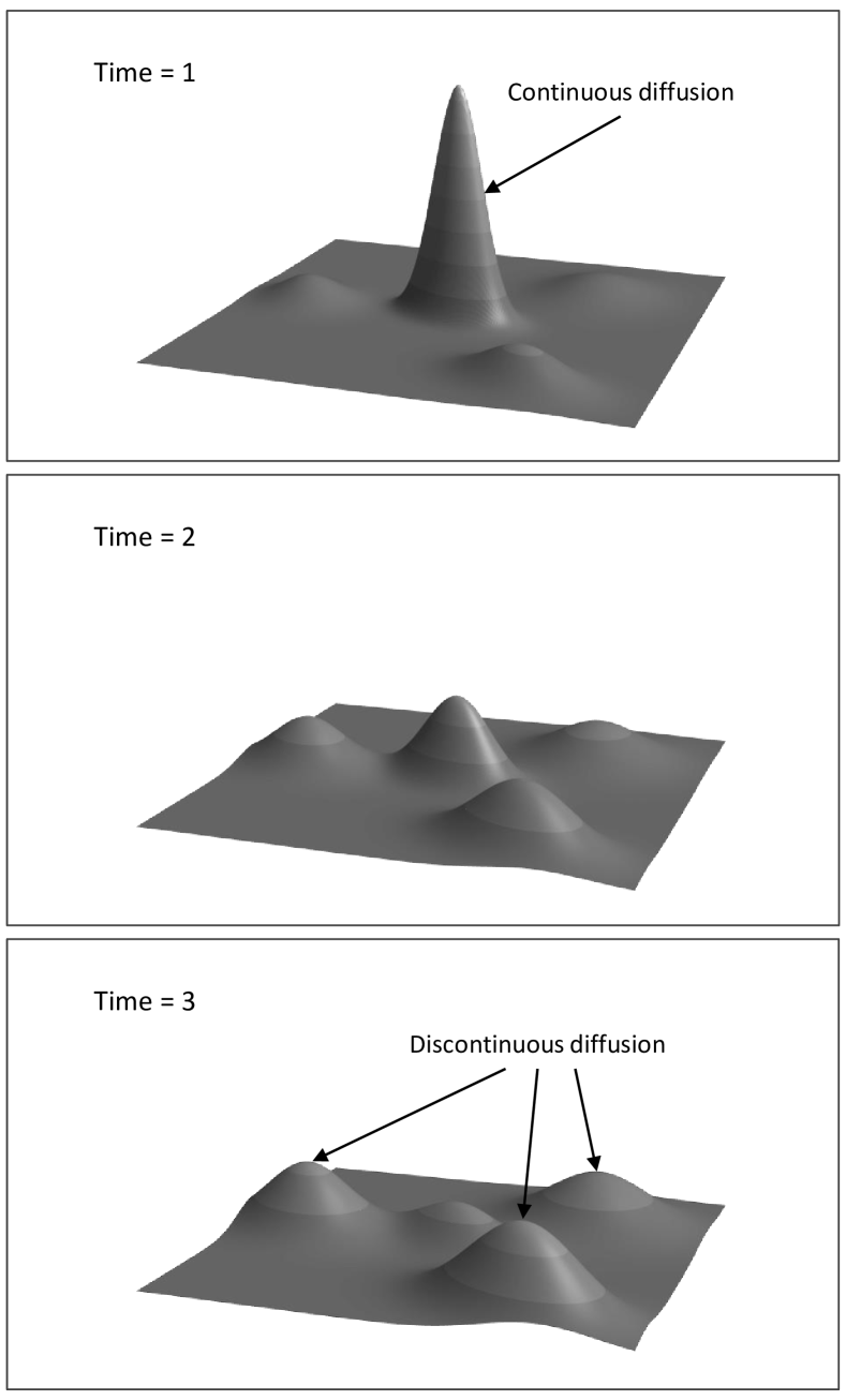
Figure 5: The evolution of the continuous-time process has a continuous component described by its mean and covariance rates and a discontinuous component described by the frequency of jumps of different sizes.

The technical conditions that enable the perpetual subdivision of a process are captured in the Lévy-Khintchine representation of its stochastic differential equation. The evolution of the continuous-time vector process $\mathsf{s}$ in the measure $\mathsf{z}$ is described by its volatility parameters $(\mu,\nu,\phi)$, where $\mu$ and $\nu$ are the rates of change for the mean and covariance in the continuous diffusion, and $\phi$ is the frequency density for jumps in the discontinuous diffusion. The Lévy-Khintchine representation of the stochastic differential equation is then:

$$\frac{\log\mathsf{z}\bullet\exp[k\cdot d\mathsf{s}]}{dt}=$$ (59)

$$\hskip 28.45274ptk\cdot\mu+\frac{1}{2}k\cdot\nu k+\int(\exp[k\cdot j]-1)\phi[j]\,dj+O[dt]$$

The continuous diffusion captures the normal conditions of the evolution, whose behaviour is accurately described over short intervals by the mean and covariance in a Gauss distribution for the increment. The discontinuous diffusion adjusts the skew and kurtosis and other higher moments of the incremental distribution, and enables the modelling of regime switches where the normal correlations between state variables are inverted.

Differentiating the stochastic differential equation repeatedly with respect to the conjugate variable $k$ brings down a power of the increment $d\mathsf{s}$ in the integrand. This observation is used to identify the stochastic differential equation for the derived process $f[t,\mathsf{s}]$ as a function of time and the state process:

$$\frac{\log\mathsf{z}\bullet\exp[k\,df[t,\mathsf{s}]]}{dt}=$$ (60)

$$\hskip 28.45274ptk(\dot{f}[t,\mathsf{s}]+f^{\prime}[t,\mathsf{s}]\cdot\mu+\frac{1}{2}\mathop{\mathrm{t}r}[f^{\prime\prime}[t,\mathsf{s}]\nu])+\frac{1}{2}k^{2}f^{\prime}[t,\mathsf{s}]\cdot\nu f^{\prime}[t,\mathsf{s}]$$

$$\hskip 28.45274pt+\int(\exp[k(f[t,\mathsf{s}+j]-f[t,\mathsf{s}])]-1)\phi[j]\,dj+O[dt]$$

This is the Itô lemma in the Lévy-Khintchine representation. Applications of the lemma transform the analysis of continuous-time processes into the realm of partial differential-integral equations, and are used in the following to derive hedge strategies and fair pricing conditions for continuously-settled derivatives.

5.1 Market and funding convexity

The price model is based on the increments $d(\mathsf{p}/\mathsf{q})$ and $d(\mathsf{a}/\mathsf{b})$ for the price ratios of underlying and derivative securities and the increments $d(\mathsf{q}/\mathsf{u})$ and $d(\mathsf{b}/\mathsf{u})$ for the ratios of the corresponding funding prices over the unsecured funding price. These increments are modelled in the economic measure $\mathsf{\bar{z}}$ by their combined stochastic differential equation in the Lévy-Khintchine representation, enabling the construction of optimal hedge strategies and the fair pricing condition from the volatility parameters. The model then captures the market convexity arising from nonlinearity in the relationships between market prices and the funding convexity resulting from differences in funding arrangements.

To reduce the dimensionality of the problem, in this section it is assumed that the underlying and derivative securities have the same funding price:

$$\mathsf{q}=\mathsf{b}=\mathsf{fu}$$ (61)

scaling the unsecured funding price by the strictly-positive funding ratio $\mathsf{f}$. This simplification puts the focus primarily on market convexity. The neglected convexities between underlying and derivative funding can be accommodated in the framework by extending the volatility parameters to allow decorrelation between the funding prices.

The joint evolution for the funding ratio $\mathsf{f}$ and the price ratios $\mathsf{s}=\mathsf{p}/\mathsf{q}$ and $\mathsf{c}=\mathsf{a}/\mathsf{b}$ of underlying and derivative securities is modelled in the economic measure $\mathsf{\bar{z}}$ by the stochastic differential equation:

$$\frac{\log\mathsf{\bar{z}}\bullet\exp[k_{\mathsf{f}}\,d\mathsf{f}/\mathsf{f}+k_{\mathsf{s}}\cdot d\mathsf{s}+k_{\mathsf{c}}\,d\mathsf{c}]}{dt}=$$ (62)

$$\hskip 28.45274pt\begin{bmatrix}k_{\mathsf{f}}\\ k_{\mathsf{s}}\\ k_{\mathsf{c}}\end{bmatrix}\cdot\begin{bmatrix}\mu_{\mathsf{f}}\\ \mu_{\mathsf{s}}\\ \mu_{\mathsf{c}}\end{bmatrix}+\frac{1}{2}\begin{bmatrix}k_{\mathsf{f}}\\ k_{\mathsf{s}}\\ k_{\mathsf{c}}\end{bmatrix}\cdot\begin{bmatrix}\nu_{\mathsf{f}}&\nu_{\mathsf{fs}}^{t}&\nu_{\mathsf{fc}}\\ \nu_{\mathsf{fs}}&\nu_{\mathsf{s}}&\nu_{\mathsf{sc}}\\ \nu_{\mathsf{fc}}&\nu_{\mathsf{sc}}^{t}&\nu_{\mathsf{c}}\end{bmatrix}\begin{bmatrix}k_{\mathsf{f}}\\ k_{\mathsf{s}}\\ k_{\mathsf{c}}\end{bmatrix}$$

$$\hskip 28.45274pt+\int(\exp[k_{\mathsf{f}}j_{\mathsf{f}}+k_{\mathsf{s}}\cdot j_{\mathsf{s}}+k_{\mathsf{c}}j_{\mathsf{c}}]-1)\phi[j_{\mathsf{f}},j_{\mathsf{s}},j_{\mathsf{c}}]\,dj_{\mathsf{f}}\,dj_{\mathsf{s}}\,dj_{\mathsf{c}}+O[dt]$$

The continuous diffusion is described by the mean rates $\mu_{\mathsf{f}}$, $\mu_{\mathsf{s}}$ and $\mu_{\mathsf{c}}$ and the covariance rates $\nu_{\mathsf{f}}$, $\nu_{\mathsf{s}}$ and $\nu_{\mathsf{c}}$ of the funding and price ratios, together with the cross-covariance rates $\nu_{\mathsf{fs}}$, $\nu_{\mathsf{fc}}$ and $\nu_{\mathsf{sc}}$ between them. The discontinuous diffusion is described by the frequency density $\phi[j_{\mathsf{f}},j_{\mathsf{s}},j_{\mathsf{c}}]$ for jumps $j_{\mathsf{f}}$, $j_{\mathsf{s}}$ and $j_{\mathsf{c}}$ in the funding and price ratios.

The model is used to generate statistics in the equivalent measure $\mathsf{\bar{z}}[\alpha]$, where the parameters $\alpha$ that adjust the economic measure will be used to mark the model to market. The returns $\mathsf{R}_{\mathsf{p}}$ and $\mathsf{R}_{\mathsf{a}}$ are expressed in terms of the increments $d\mathsf{f}/\mathsf{f}$, $d\mathsf{s}$ and $d\mathsf{c}$:

$$\mathsf{R}_{\mathsf{p}}=\mathsf{f}(1+\frac{d\mathsf{f}}{\mathsf{f}})\,d\mathsf{s\hskip 28.45274ptR}_{\mathsf{a}}=\mathsf{f}(1+\frac{d\mathsf{f}}{\mathsf{f}})\,d\mathsf{c}$$ (63)

The statistics for the underlying and derivative are encapsulated in the stochastic differential equation for the returns as the coefficients in its series expansion with respect to the conjugate variables. The Itô lemma derives the expression:

$$\frac{\log\mathsf{\bar{z}}[\alpha]\bullet\exp[k_{\mathsf{p}}\cdot\mathsf{R}_{\mathsf{p}}+k_{\mathsf{a}}\mathsf{R}_{\mathsf{a}}]}{dt}=$$ (64)

$$\hskip 28.45274pt\mathsf{f}(k_{\mathsf{p}}\cdot(\mu_{\mathsf{s}}[\alpha]+\nu_{\mathsf{fs}})+k_{\mathsf{a}}(\mu_{\mathsf{c}}[\alpha]+\nu_{\mathsf{fc}}))$$

$$\hskip 28.45274pt+\mathsf{f}^{2}(\frac{1}{2}k_{\mathsf{p}}\cdot\nu_{\mathsf{s}}k_{\mathsf{p}}+\frac{1}{2}k_{\mathsf{a}}^{2}\nu_{\mathsf{c}}+k_{\mathsf{a}}k_{\mathsf{p}}\cdot\nu_{\mathsf{sc}})$$

$$\hskip 28.45274pt+\int(\exp[\mathsf{f}(1+j_{\mathsf{f}})(k_{\mathsf{p}}\cdot j_{\mathsf{s}}+k_{\mathsf{a}}j_{\mathsf{c}})]-1)\phi[\alpha][j_{\mathsf{f}},j_{\mathsf{s}},j_{\mathsf{c}}]\,dj_{\mathsf{f}}\,dj_{\mathsf{s}}\,dj_{\mathsf{c}}+O[dt]$$

with adjusted volatility parameters:

$$\mu_{\mathsf{s}}[\alpha] =\mu_{\mathsf{s}}-\nu_{\mathsf{s}}\mathsf{f}\alpha$$ (65)

$$\mu_{\mathsf{c}}[\alpha] =\mu_{\mathsf{c}}-\mathsf{f}\alpha\cdot\nu_{\mathsf{sc}}$$

$$\phi[\alpha][j_{\mathsf{f}},j_{\mathsf{s}},j_{\mathsf{c}}] =\exp[-\mathsf{f}(1+j_{\mathsf{f}})\alpha\cdot j_{\mathsf{s}}]\phi[j_{\mathsf{f}},j_{\mathsf{s}},j_{\mathsf{c}}]$$

The performance of the hedge strategy and the fair price of the derivative are determined using the first and second moments extracted from this equation.

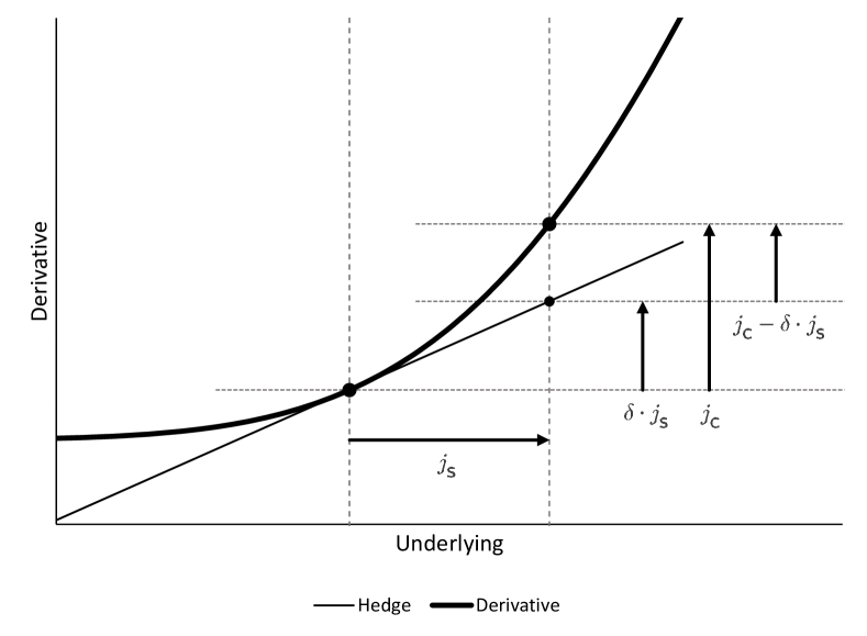
Figure 6: The delta hedge matches the continuous price movements for the derivative with an offsetting position in the underlying. Discontinuous price movements invalidate the hedge when there is convexity in the relationship between the underlying and derivative prices.

The covariances of the returns in the measure $\mathsf{\bar{z}}[\alpha]$ are:

$$\begin{bmatrix}\mathsf{V}_{\mathsf{p}}[\alpha]&\mathsf{C}_{\mathsf{pa}}[\alpha]\\ \mathsf{C}_{\mathsf{pa}}^{t}[\alpha]&\mathsf{V}_{\mathsf{a}}[\alpha]\end{bmatrix}=\mathsf{f}^{2}\begin{bmatrix}\mathsf{\dot{V}}_{\mathsf{s}}[\alpha]&\mathsf{\dot{C}}_{\mathsf{sc}}[\alpha]\\ \mathsf{\dot{C}}_{\mathsf{sc}}^{t}[\alpha]&\mathsf{\dot{V}}_{\mathsf{c}}[\alpha]\end{bmatrix}dt+O[dt^{2}]$$ (66)

where the variance rates are given by:

$$\mathsf{\dot{V}}_{\mathsf{s}}[\alpha] =\nu_{\mathsf{s}}+\int(1+j_{\mathsf{f}})^{2}j_{\mathsf{s}}^{2}\phi[\alpha][j_{\mathsf{f}},j_{\mathsf{s}},j_{\mathsf{c}}]\,dj_{\mathsf{f}}\,dj_{\mathsf{s}}\,dj_{\mathsf{c}}$$ (67)

$$\mathsf{\dot{V}}_{\mathsf{c}}[\alpha] =\nu_{\mathsf{c}}+\int(1+j_{\mathsf{f}})^{2}j_{\mathsf{c}}^{2}\phi[\alpha][j_{\mathsf{f}},j_{\mathsf{s}},j_{\mathsf{c}}]\,dj_{\mathsf{f}}\,dj_{\mathsf{s}}\,dj_{\mathsf{c}}$$

and the covariance rate is given by:

$$\mathsf{\dot{C}}_{\mathsf{sc}}[\alpha]=\nu_{\mathsf{sc}}+\int(1+j_{\mathsf{f}})^{2}j_{\mathsf{s}}j_{\mathsf{c}}\phi[\alpha][j_{\mathsf{f}},j_{\mathsf{s}},j_{\mathsf{c}}]\,dj_{\mathsf{f}}\,dj_{\mathsf{s}}\,dj_{\mathsf{c}}$$ (68)

The optimal hedge strategy minimises the variance for the return on the hedged derivative. Quantifying performance using the equivalent measure with parameters $\alpha$, the optimal hedge weights are:

$$\beta=\mathsf{\dot{V}}_{\mathsf{s}}[\alpha]^{-1}\mathsf{\dot{C}}_{\mathsf{sc}}[\alpha]+O[dt]$$ (69)

This strategy does not necessarily eliminate the market risk of the hedged derivative. The residual variance of the hedged portfolio is calculated as:

$$\mathsf{v}=\mathsf{f}^{2}(\mathsf{\dot{V}}_{\mathsf{c}}[\alpha]-\mathsf{\dot{V}}_{\mathsf{s}}[\alpha]^{-1}\mathsf{\dot{C}}_{\mathsf{sc}}[\alpha]\cdot\mathsf{\dot{C}}_{\mathsf{sc}}[\alpha])\,dt+O[dt]$$ (70)

including contributions from the continuous and discontinuous components of the price diffusion. The hedge strategy strikes a balance between these contributions, optimising against both the infinitesimal price moves of the continuous diffusion and the discrete price moves of the discontinuous diffusion according to their relative likelihoods.

The continuous contribution dominates when $J^{2}\Phi$ is small, where $J$ is the maximum size of jumps in the support of the frequency density and $\Phi$ is the total frequency. The optimal hedge expands as:

$$\beta=\delta+\gamma+O[dt]$$ (71)

The contribution $\delta$ from the continuous diffusion is the delta hedge against infinitesimal changes in the prices, and this is corrected by the adjustment $\gamma$ that accounts for the discontinuous diffusion:

$$\delta =\nu_{\mathsf{s}}^{-1}\nu_{\mathsf{sc}}$$ (72)

$$\gamma =\int(1+j_{\mathsf{f}})^{2}(j_{\mathsf{c}}-\delta\cdot j_{\mathsf{s}})(\nu_{\mathsf{s}}^{-1}j_{\mathsf{s}})\phi[\alpha][j_{\mathsf{f}},j_{\mathsf{s}},j_{\mathsf{c}}]\,dj_{\mathsf{f}}\,dj_{\mathsf{s}}\,dj_{\mathsf{c}}+O[(J^{2}\Phi)^{2}]$$

Price discontinuities corrupt the delta hedge strategy when there is convexity in the relationship between underlying and derivative, requiring a correction to the strategy in proportion to the deviation $(j_{\mathsf{c}}-\delta\cdot j_{\mathsf{s}})$ from the linear approximation. The delta hedge does not depend on the parameters $\alpha$ that adjust the economic measure, nor is it impacted by the volatility of the funding ratio. Sensitivities to these elements are only introduced when there is indeterminacy in the size and direction of the underlying and derivative price jumps.

The means of the returns in the measure $\mathsf{\bar{z}}[\alpha]$ are:

$$\begin{bmatrix}\mathsf{M}_{\mathsf{p}}[\alpha]\\ \mathsf{M}_{\mathsf{a}}[\alpha]\end{bmatrix}=\mathsf{f}\begin{bmatrix}\mathsf{\dot{M}}_{\mathsf{s}}[\alpha]\\ \mathsf{\dot{M}}_{\mathsf{c}}[\alpha]\end{bmatrix}dt+O[dt^{2}]$$ (73)

where the mean rates are given by:

$$\mathsf{\dot{M}}_{\mathsf{s}}[\alpha] =\mu_{\mathsf{s}}[\alpha]+\nu_{\mathsf{fs}}+\int(1+j_{\mathsf{f}})j_{\mathsf{s}}\phi[\alpha][j_{\mathsf{f}},j_{\mathsf{s}},j_{\mathsf{c}}]\,dj_{\mathsf{f}}\,dj_{\mathsf{s}}\,dj_{\mathsf{c}}$$ (74)

$$\mathsf{\dot{M}}_{\mathsf{c}}[\alpha] =\mu_{\mathsf{c}}[\alpha]+\nu_{\mathsf{fc}}+\int(1+j_{\mathsf{f}})j_{\mathsf{c}}\phi[\alpha][j_{\mathsf{f}},j_{\mathsf{s}},j_{\mathsf{c}}]\,dj_{\mathsf{f}}\,dj_{\mathsf{s}}\,dj_{\mathsf{c}}$$

The price model derived from the maximum entropy principle assumes the mean of the derivative return is zero in the price measure that calibrates the parameters $\alpha$ so that the means of the underlying returns are also zero:

$$\mathsf{\dot{M}}_{\mathsf{s}}[\alpha] =0$$ (75)

$$\mathsf{\dot{M}}_{\mathsf{c}}[\alpha] =0$$

The calibration constraint is solved for the parameters that are then used in the price equation for the derivative. These expressions simplify when the underlying price diffusion is continuous, so that the frequency density takes the form:

$$\phi[j_{\mathsf{f}},j_{\mathsf{s}},j_{\mathsf{c}}]=\delta[j_{\mathsf{s}}]\phi[j_{\mathsf{f}},j_{\mathsf{c}}]$$ (76)

In this case, the solution for the parameters is entered into the condition for the derivative return to generate the price equation:

$$\mu_{\mathsf{c}}+\nu_{\mathsf{fc}}+\int(1+j_{\mathsf{f}})j_{\mathsf{c}}\phi[j_{\mathsf{f}},j_{\mathsf{c}}]\,dj_{\mathsf{f}}\,dj_{\mathsf{c}}=\nu_{\mathsf{s}}^{-1}\nu_{\mathsf{sc}}\cdot(\mu_{\mathsf{s}}+\nu_{\mathsf{fs}})$$ (77)

identifying the drift of the derivative price.

The assumption of continuous diffusion for the underlying prices can be reasonable in benign market conditions. Liquidity is a desirable property of market hedge instruments, and the price transparency and trading volumes on exchanges facilitate continuous hedging. In stressed conditions, or for hedging with less liquid instruments, the economic model should reflect the potential difficulties with continuous hedging by incorporating a discontinuous component for the underlying price diffusion. The calibration parameters are then determined from the underlying drift condition via the Newton-Raphson scheme.

5.2 Stochastic volatility

In the previous section, the drift conditions for the underlying and derivative returns are derived from the maximum entropy principle on the assumption of continuous margin settlement. The approach is demonstrated in this section by considering in detail the economic model:

$$\frac{\log\mathsf{\bar{z}}\bullet\exp[k_{\mathsf{s}}\,d\mathsf{s}+k_{\boldsymbol{\sigma}}\cdot d\boldsymbol{\sigma}]}{dt}=$$ (78)

$$\hskip 28.45274ptk_{\mathsf{s}}\mu_{\mathsf{s}}+k_{\boldsymbol{\sigma}}\cdot\mu_{\boldsymbol{\sigma}}+\frac{1}{2}k_{\mathsf{s}}^{2}\nu_{\mathsf{s}}+\frac{1}{2}k_{\boldsymbol{\sigma}}\cdot\nu_{\boldsymbol{\sigma}}k_{\boldsymbol{\sigma}}+k_{\mathsf{s}}k_{\boldsymbol{\sigma}}\cdot\nu_{\mathsf{s}\boldsymbol{\sigma}}$$

$$\hskip 28.45274pt+\int(\exp[k_{\mathsf{s}}j_{\mathsf{s}}+k_{\boldsymbol{\sigma}}\cdot j_{\boldsymbol{\sigma}}]-1)\phi[j_{\mathsf{s}},j_{\boldsymbol{\sigma}}]\,dj_{\mathsf{s}}\,dj_{\boldsymbol{\sigma}}+O[dt]$$

describing the evolution in the economic measure of a single underlying price $\mathsf{s}$ and an additional state vector $\boldsymbol{\sigma}$ used to model its volatility. Funding convexity is neglected by setting $\mathsf{f}=1$, and the mean rates $\mu_{\mathsf{s}}$ and $\mu_{\boldsymbol{\sigma}}$, covariance rates $\nu_{\mathsf{s}}$, $\nu_{\boldsymbol{\sigma}}$ and $\nu_{\mathsf{s}\boldsymbol{\sigma}}$, and jump frequency $\phi[j_{\mathsf{s}},j_{\boldsymbol{\sigma}}]$ are all assumed to be functions of time $t$ and the state variables $\mathsf{s}$ and $\boldsymbol{\sigma}$. Many popular models for pricing derivatives are included in this setup.

Black-Scholes-Merton model:

This model assumes a stationary evolution for the underlying price with constant volatility:

$$\frac{\log\mathsf{\bar{z}}\bullet\exp[k_{\mathsf{s}}\,d\mathsf{s}/\mathsf{s}]}{dt}=$$ (79)

$$\hskip 28.45274ptk_{\mathsf{s}}\mu+\frac{1}{2}k_{\mathsf{s}}^{2}\sigma^{2}+\int_{j=-1}^{\infty}(\exp[k_{\mathsf{s}}j]-1)\psi[j]\,dj+O[dt]$$

The model parameters are the mean rate $\mu$, the volatility rate $\sigma$, and the frequency of jumps $\psi[j]$ for the underlying price.

Heston model:

This model assumes a stationary evolution for the underlying price with stochastic volatility following a correlated square-root process:

$$\frac{\log\mathsf{\bar{z}}\bullet\exp[k_{\mathsf{s}}\,d\mathsf{s}/\mathsf{s}+k_{\boldsymbol{\nu}}\,d\boldsymbol{\nu}]}{dt}=$$ (80)

$$\hskip 28.45274ptk_{\mathsf{s}}\mu+k_{\boldsymbol{\nu}}\kappa(\theta-\boldsymbol{\nu})+\frac{1}{2}k_{\mathsf{s}}^{2}\boldsymbol{\nu}+\frac{1}{2}k_{\boldsymbol{\nu}}^{2}\xi^{2}\boldsymbol{\nu}+k_{\mathsf{s}}k_{\boldsymbol{\nu}}\rho\xi\boldsymbol{\nu}+O[dt]$$

The additional state variable $\boldsymbol{\nu}$ is interpreted as the instantaneous variance of the underlying price. The model parameters are the mean rate $\mu$ of the underlying price, the mean reversion rate $\kappa$ and reversion level $\theta$ of the variance, the volatility of variance $\xi$, and the correlation $\rho$ between the price and its variance.

SABR model:

This model assumes the underlying price has constant elasticity of variance with stochastic volatility following a correlated lognormal process:

$$\frac{\log\mathsf{\bar{z}}\bullet\exp[k_{\mathsf{s}}\,d\mathsf{s}+k_{\boldsymbol{\sigma}}\,d\boldsymbol{\sigma}+k_{\boldsymbol{\alpha}}\,d\boldsymbol{\alpha}+k_{\boldsymbol{\beta}}\,d\boldsymbol{\beta}+k_{\boldsymbol{\rho}}\,d\boldsymbol{\rho}]}{dt}=$$ (81)

$$\hskip 28.45274pt\frac{1}{2}k_{\mathsf{s}}^{2}\boldsymbol{\sigma}^{2}\mathsf{s}^{2\boldsymbol{\beta}}+\frac{1}{2}k_{\boldsymbol{\sigma}}^{2}\boldsymbol{\alpha}^{2}\boldsymbol{\sigma}^{2}+k_{\mathsf{s}}k_{\boldsymbol{\sigma}}\boldsymbol{\rho\alpha\sigma}^{2}\mathsf{s}^{\boldsymbol{\beta}}+O[dt]$$

The additional state variables are the instantaneous volatility $\boldsymbol{\sigma}$ of the underlying price, the volatility of volatility $\boldsymbol{\alpha}$, the elasticity of variance $\boldsymbol{\beta}$, and the correlation $\boldsymbol{\rho}$ between the price and its volatility.

The maximum entropy principle locates the price measure $\mathsf{\hat{z}}$ among the equivalent measures $\mathsf{\bar{z}}[\alpha]$ parametrised by the weight $\alpha$ for the underlying return. The evolution of the state variables in this measure is modelled by:

$$\frac{\log\mathsf{\bar{z}}[\alpha]\bullet\exp[k_{\mathsf{s}}\,d\mathsf{s}+k_{\boldsymbol{\sigma}}\cdot d\boldsymbol{\sigma}]}{dt}=$$ (82)

$$\hskip 28.45274ptk_{\mathsf{s}}\mu_{\mathsf{s}}[\alpha]+k_{\boldsymbol{\sigma}}\cdot\mu_{\boldsymbol{\sigma}}[\alpha]+\frac{1}{2}k_{\mathsf{s}}^{2}\nu_{\mathsf{s}}+\frac{1}{2}k_{\boldsymbol{\sigma}}\cdot\nu_{\boldsymbol{\sigma}}k_{\boldsymbol{\sigma}}+k_{\mathsf{s}}k_{\boldsymbol{\sigma}}\cdot\nu_{\mathsf{s}\boldsymbol{\sigma}}$$

$$\hskip 28.45274pt+\int(\exp[k_{\mathsf{s}}j_{\mathsf{s}}+k_{\boldsymbol{\sigma}}\cdot j_{\boldsymbol{\sigma}}]-1)\phi[\alpha][j_{\mathsf{s}},j_{\boldsymbol{\sigma}}]\,dj_{\mathsf{s}}\,dj_{\boldsymbol{\sigma}}+O[dt]$$

with adjusted parameters:

$$\mu_{\mathsf{s}}[\alpha] =\mu_{\mathsf{s}}-\alpha\nu_{\mathsf{s}}$$ (83)

$$\mu_{\boldsymbol{\sigma}}[\alpha] =\mu_{\boldsymbol{\sigma}}-\alpha\nu_{\mathsf{s}\boldsymbol{\sigma}}$$

$$\phi[\alpha][j_{\mathsf{s}},j_{\boldsymbol{\sigma}}] =\exp[-\alpha j_{\mathsf{s}}]\phi[j_{\mathsf{s}},j_{\boldsymbol{\sigma}}]$$

These adjustments modify the mean rates and jump frequency of the price diffusion via the control variable $\alpha$, which is used to calibrate the price measure to the underlying returns.

Market completeness for the derivative depends on the availability of hedge securities and the nature of their joint price dynamics. In the following, hedge strategies are considered for the derivative with price $\mathsf{c}=c[t,\mathsf{s},\boldsymbol{\sigma}]$ expressed as a function of time and the state variables. Hedging with only the underlying neglects the contributions to volatility from the additional state variables, leaving residual risk in the portfolio. Hedge performance is improved if the market includes options on the underlying that mark the state variables.

In the incomplete hedging scenario, the returns on the hedge and derivative securities are:

$$\mathsf{R}_{\mathsf{p}}=d\mathsf{s\hskip 28.45274ptR}_{\mathsf{a}}=d\mathsf{c}$$ (84)

The means of the returns in the equivalent measure $\mathsf{\bar{z}}[\alpha]$ are:

$$\begin{bmatrix}\mathsf{M}_{\mathsf{p}}[\alpha]\\ \mathsf{M}_{\mathsf{a}}[\alpha]\end{bmatrix}=\begin{bmatrix}\mathsf{\dot{M}}_{\mathsf{s}}[\alpha]\\ \mathsf{\dot{M}}_{\mathsf{c}}[\alpha]\end{bmatrix}dt+O[dt^{2}]$$ (85)

where the mean rates are given by:

$$\mathsf{\dot{M}}_{\mathsf{s}}[\alpha]=\, \mu_{\mathsf{s}}[\alpha]+\int j_{\mathsf{s}}\phi[\alpha][j_{\mathsf{s}},j_{\boldsymbol{\sigma}}]\,dj_{\mathsf{s}}\,dj_{\boldsymbol{\sigma}}$$ (86)

$$\mathsf{\dot{M}}_{\mathsf{c}}[\alpha]=\, \frac{\partial c}{\partial t}+\frac{\partial c}{\partial\mathsf{s}}\mu_{\mathsf{s}}[\alpha]+\frac{\partial c}{\partial\boldsymbol{\sigma}}\cdot\mu_{\boldsymbol{\sigma}}[\alpha]+\frac{1}{2}\frac{\partial^{2}c}{\partial\mathsf{s}^{2}}\nu_{\mathsf{s}}+\frac{1}{2}\mathop{\mathrm{t}r}[\frac{\partial^{2}c}{\partial\boldsymbol{\sigma}^{2}}\nu_{\boldsymbol{\sigma}}]+\frac{\partial^{2}c}{\partial\mathsf{s}\partial\boldsymbol{\sigma}}\cdot\nu_{\mathsf{s}\boldsymbol{\sigma}}$$

$$+\int j_{\mathsf{c}}\phi[\alpha][j_{\mathsf{s}},j_{\boldsymbol{\sigma}}]\,dj_{\mathsf{s}}\,dj_{\boldsymbol{\sigma}}$$

The jump $j_{\mathsf{c}}$ for the derivative price, appearing in the integrand of the discontinuous contribution, is defined in terms of the jumps $j_{\mathsf{s}}$ and $j_{\boldsymbol{\sigma}}$ for the underlying price and state variables:

$$j_{\mathsf{c}}=c[t,\mathsf{s}+j_{\mathsf{s}},\boldsymbol{\sigma}+j_{\boldsymbol{\sigma}}]-c[t,\mathsf{s},\boldsymbol{\sigma}]$$ (87)

The equation for the fair price of the derivative is obtained by setting the means of the underlying and derivative returns to zero in the price measure $\mathsf{\hat{z}}=\mathsf{\bar{z}}[\alpha]$, with the first condition used to calibrate the weight $\alpha$ that is then applied in the second condition to determine the derivative price:

$$0=\, \mu_{\mathsf{s}}-\alpha\nu_{\mathsf{s}}+\int j_{\mathsf{s}}\exp[-\alpha j_{\mathsf{s}}]\phi[j_{\mathsf{s}},j_{\boldsymbol{\sigma}}]\,dj_{\mathsf{s}}\,dj_{\boldsymbol{\sigma}}$$ (88)

$$0=\, \frac{\partial c}{\partial t}+\frac{\partial c}{\partial\boldsymbol{\sigma}}\cdot(\mu_{\boldsymbol{\sigma}}-\alpha\nu_{\mathsf{s}\boldsymbol{\sigma}})+\frac{1}{2}\frac{\partial^{2}c}{\partial\mathsf{s}^{2}}\nu_{\mathsf{s}}+\frac{1}{2}\mathop{\mathrm{t}r}[\frac{\partial^{2}c}{\partial\boldsymbol{\sigma}^{2}}\nu_{\boldsymbol{\sigma}}]+\frac{\partial^{2}c}{\partial\mathsf{s}\partial\boldsymbol{\sigma}}\cdot\nu_{\mathsf{s}\boldsymbol{\sigma}}$$

$$+\int(j_{\mathsf{c}}-\frac{\partial c}{\partial\mathsf{s}}j_{\mathsf{s}})\exp[-\alpha j_{\mathsf{s}}]\phi[j_{\mathsf{s}},j_{\boldsymbol{\sigma}}]\,dj_{\mathsf{s}}\,dj_{\boldsymbol{\sigma}}$$

These expressions simplify when the underlying price diffusion is continuous, so that the frequency density takes the form:

$$\phi[j_{\mathsf{s}},j_{\boldsymbol{\sigma}}]=\delta[j_{\mathsf{s}}]\phi[j_{\boldsymbol{\sigma}}]$$ (89)

In this case, the calibration constraint is solved by $\alpha=\mu_{\mathsf{s}}/\nu_{\mathsf{s}}$, and the price equation becomes:

$$0=\, \frac{\partial c}{\partial t}+\frac{\partial c}{\partial\boldsymbol{\sigma}}\cdot(\mu_{\boldsymbol{\sigma}}-\frac{\mu_{\mathsf{s}}}{\nu_{\mathsf{s}}}\nu_{\mathsf{s}\boldsymbol{\sigma}})+\frac{1}{2}\frac{\partial^{2}c}{\partial\mathsf{s}^{2}}\nu_{\mathsf{s}}+\frac{1}{2}\mathop{\mathrm{t}r}[\frac{\partial^{2}c}{\partial\boldsymbol{\sigma}^{2}}\nu_{\boldsymbol{\sigma}}]+\frac{\partial^{2}c}{\partial\mathsf{s}\partial\boldsymbol{\sigma}}\cdot\nu_{\mathsf{s}\boldsymbol{\sigma}}$$ (90)

$$+\int j_{\mathsf{c}}\phi[j_{\boldsymbol{\sigma}}]\,dj_{\boldsymbol{\sigma}}$$

The partial differential-integral equation for the fair price of the derivative is solved against the boundary conditions provided by the terminal settlements, as specified in the derivative contract.

Now suppose that the hedge market includes options on the underlying, with prices $\mathsf{o}=o[t,\mathsf{s},\boldsymbol{\sigma}]$ expressed as functions of time and the state variables. Further assume that the options mark the additional state variables, with implied volatility function $\boldsymbol{\sigma}=\sigma[t,\mathsf{s},\mathsf{o}]$ satisfying:

$$\sigma[t,\mathsf{s},o[t,\mathsf{s},\boldsymbol{\sigma}]] =\boldsymbol{\sigma}$$ (91)

$$o[t,\mathsf{s},\sigma[t,\mathsf{s},\mathsf{o}]] =\mathsf{o}$$

These options enable the hedging of all the state variables, thereby reducing the residual risk of the hedged derivative.

In the complete hedging scenario, the returns on the hedge and derivative securities are:

$$\mathsf{R}_{\mathsf{p}}=\begin{bmatrix}d\mathsf{s}\\ d\mathsf{o}\end{bmatrix}\mathsf{\hskip 28.45274ptR}_{\mathsf{a}}=d\mathsf{c}$$ (92)

The covariances of the returns in the economic measure $\mathsf{\bar{z}}$ are:

$$\begin{bmatrix}\mathsf{V}_{\mathsf{p}}&\mathsf{C}_{\mathsf{pa}}\\ \mathsf{C}_{\mathsf{pa}}^{t}&\mathsf{V}_{\mathsf{a}}\end{bmatrix}=\begin{bmatrix}\mathsf{\dot{V}}_{\mathsf{s}}&\mathsf{\dot{C}}_{\mathsf{so}}^{t}&\mathsf{\dot{C}}_{\mathsf{sc}}\\ \mathsf{\dot{C}}_{\mathsf{so}}&\mathsf{\dot{V}}_{\mathsf{o}}&\mathsf{\dot{C}}_{\mathsf{oc}}\\ \mathsf{\dot{C}}_{\mathsf{sc}}&\mathsf{\dot{C}}_{\mathsf{oc}}^{t}&\mathsf{\dot{V}}_{\mathsf{c}}\end{bmatrix}dt+O[dt^{2}]$$ (93)

where the variance rates are given by:

$$\mathsf{\dot{V}}_{\mathsf{s}} =\nu_{\mathsf{s}}+\int j_{\mathsf{s}}^{2}\phi[j_{\mathsf{s}},j_{\boldsymbol{\sigma}}]\,dj_{\mathsf{s}}\,dj_{\boldsymbol{\sigma}}$$ (94)

$$\mathsf{\dot{V}}_{\mathsf{o}} =(\frac{\partial o}{\partial\mathsf{s}})^{2}\nu_{\mathsf{s}}+\frac{\partial o}{\partial\boldsymbol{\sigma}}\cdot\nu_{\boldsymbol{\sigma}}\frac{\partial o}{\partial\boldsymbol{\sigma}}+2\frac{\partial o}{\partial\mathsf{s}}\frac{\partial o}{\partial\boldsymbol{\sigma}}\cdot\nu_{\mathsf{s}\boldsymbol{\sigma}}+\int j_{\mathsf{o}}^{2}\phi[j_{\mathsf{s}},j_{\boldsymbol{\sigma}}]\,dj_{\mathsf{s}}\,dj_{\boldsymbol{\sigma}}$$

$$\mathsf{\dot{V}}_{\mathsf{c}} =(\frac{\partial c}{\partial\mathsf{s}})^{2}\nu_{\mathsf{s}}+\frac{\partial c}{\partial\boldsymbol{\sigma}}\cdot\nu_{\boldsymbol{\sigma}}\frac{\partial c}{\partial\boldsymbol{\sigma}}+2\frac{\partial c}{\partial\mathsf{s}}\frac{\partial c}{\partial\boldsymbol{\sigma}}\cdot\nu_{\mathsf{s}\boldsymbol{\sigma}}+\int j_{\mathsf{c}}^{2}\phi[j_{\mathsf{s}},j_{\boldsymbol{\sigma}}]\,dj_{\mathsf{s}}\,dj_{\boldsymbol{\sigma}}$$

and the covariance rates are given by:

$$\mathsf{\dot{C}}_{\mathsf{so}} =\frac{\partial o}{\partial\mathsf{s}}\nu_{\mathsf{s}}+\frac{\partial o}{\partial\boldsymbol{\sigma}}\cdot\nu_{\mathsf{s}\boldsymbol{\sigma}}+\int j_{\mathsf{s}}j_{\mathsf{o}}\phi[j_{\mathsf{s}},j_{\boldsymbol{\sigma}}]\,dj_{\mathsf{s}}\,dj_{\boldsymbol{\sigma}}$$ (95)

$$\mathsf{\dot{C}}_{\mathsf{sc}} =\frac{\partial c}{\partial\mathsf{s}}\nu_{\mathsf{s}}+\frac{\partial c}{\partial\boldsymbol{\sigma}}\cdot\nu_{\mathsf{s}\boldsymbol{\sigma}}+\int j_{\mathsf{s}}j_{\mathsf{c}}\phi[j_{\mathsf{s}},j_{\boldsymbol{\sigma}}]\,dj_{\mathsf{s}}\,dj_{\boldsymbol{\sigma}}$$

$$\mathsf{\dot{C}}_{\mathsf{oc}} =\frac{\partial o}{\partial\mathsf{s}}\frac{\partial c}{\partial\mathsf{s}}\nu_{\mathsf{s}}+\frac{\partial o}{\partial\boldsymbol{\sigma}}\cdot\nu_{\boldsymbol{\sigma}}\frac{\partial c}{\partial\boldsymbol{\sigma}}+(\frac{\partial o}{\partial\mathsf{s}}\frac{\partial c}{\partial\boldsymbol{\sigma}}+\frac{\partial o}{\partial\boldsymbol{\sigma}}\frac{\partial c}{\partial\mathsf{s}})\cdot\nu_{\mathsf{s}\boldsymbol{\sigma}}+\int j_{\mathsf{o}}j_{\mathsf{c}}\phi[j_{\mathsf{s}},j_{\boldsymbol{\sigma}}]\,dj_{\mathsf{s}}\,dj_{\boldsymbol{\sigma}}$$

The jumps $j_{\mathsf{o}}$ and $j_{\mathsf{c}}$ for the option and derivative prices, appearing in the integrand of the discontinuous contribution, are defined in terms of the jumps $j_{\mathsf{s}}$ and $j_{\boldsymbol{\sigma}}$ for the underlying price and state variables:

$$j_{\mathsf{o}} =o[t,\mathsf{s}+j_{\mathsf{s}},\boldsymbol{\sigma}+j_{\boldsymbol{\sigma}}]-o[t,\mathsf{s},\boldsymbol{\sigma}]$$ (96)

$$j_{\mathsf{c}} =c[t,\mathsf{s}+j_{\mathsf{s}},\boldsymbol{\sigma}+j_{\boldsymbol{\sigma}}]-c[t,\mathsf{s},\boldsymbol{\sigma}]$$

Hedging with the underlying portfolio $\beta_{\mathsf{s}}$ and the option portfolio $\beta_{\mathsf{o}}$, the residual variance for the hedged derivative is:

$$\mathsf{v}=\, ((\frac{\partial c}{\partial\mathsf{s}}-\beta_{\mathsf{s}}-\beta_{\mathsf{o}}\cdot\frac{\partial o}{\partial\mathsf{s}})^{2}\nu_{\mathsf{s}}$$ (97)

$$+(\frac{\partial c}{\partial\boldsymbol{\sigma}}-\frac{\partial o}{\partial\boldsymbol{\sigma}}\beta_{\mathsf{o}})\cdot\nu_{\boldsymbol{\sigma}}(\frac{\partial c}{\partial\boldsymbol{\sigma}}-\frac{\partial o}{\partial\boldsymbol{\sigma}}\beta_{\mathsf{o}})$$

$$+2(\frac{\partial c}{\partial\mathsf{s}}-\beta_{\mathsf{s}}-\beta_{\mathsf{o}}\cdot\frac{\partial o}{\partial\mathsf{s}})(\frac{\partial c}{\partial\boldsymbol{\sigma}}-\frac{\partial o}{\partial\boldsymbol{\sigma}}\beta_{\mathsf{o}})\cdot\nu_{\mathsf{s}\boldsymbol{\sigma}}$$

$$+\int(j_{\mathsf{c}}-\beta_{\mathsf{s}}j_{\mathsf{s}}-\beta_{\mathsf{o}}\cdot j_{\mathsf{o}})^{2}\phi[j_{\mathsf{s}},j_{\boldsymbol{\sigma}}]\,dj_{\mathsf{s}}\,dj_{\boldsymbol{\sigma}})\,dt+O[dt^{2}]$$

The choice of hedge portfolio then depends on the objectives of the investor and their level of access to the hedge market. Using only the underlying, the delta hedge is:

$$\beta_{\mathsf{s}}=\frac{\partial c}{\partial\mathsf{s}}\mathsf{\hskip 28.45274pt}\beta_{\mathsf{o}}=0$$ (98)

This strategy offsets the impact on the derivative price of continuous moves in the underlying price, but neglects the impact from the volatility of state variables. The residual variance achieved by the strategy is:

$$\mathsf{v}=(\frac{\partial c}{\partial\boldsymbol{\sigma}}\cdot\nu_{\boldsymbol{\sigma}}\frac{\partial c}{\partial\boldsymbol{\sigma}}+\int(j_{\mathsf{c}}-\beta_{\mathsf{s}}j_{\mathsf{s}})^{2}\phi[j_{\mathsf{s}},j_{\boldsymbol{\sigma}}]\,dj_{\mathsf{s}}\,dj_{\boldsymbol{\sigma}})\,dt+O[dt^{2}]$$ (99)

Performance of the delta hedge is improved by including options to offset the continuous moves in the state variables:

$$\beta_{\mathsf{s}}=\frac{\partial c}{\partial\mathsf{s}}-(\frac{\partial o}{\partial\boldsymbol{\sigma}})^{-1}\frac{\partial o}{\partial\mathsf{s}}\cdot\frac{\partial c}{\partial\boldsymbol{\sigma}}\mathsf{\hskip 28.45274pt}\beta_{\mathsf{o}}=(\frac{\partial o}{\partial\boldsymbol{\sigma}})^{-1}\frac{\partial c}{\partial\boldsymbol{\sigma}}$$ (100)

This strategy removes the contribution from the continuous covariance of the underlying and option prices, leaving only the discontinuous term:

$$\mathsf{v}=(\int(j_{\mathsf{c}}-\beta_{\mathsf{s}}j_{\mathsf{s}}-\beta_{\mathsf{o}}\cdot j_{\mathsf{o}})^{2}\phi[j_{\mathsf{s}},j_{\boldsymbol{\sigma}}]\,dj_{\mathsf{s}}\,dj_{\boldsymbol{\sigma}})\,dt+O[dt^{2}]$$ (101)

The prize-winning observation is that the continuous contribution to the residual variance can be completely eliminated when there are sufficient hedge securities available to match against the volatile state variables. Moreover, the discontinuous contribution is small if the price jumps broadly align with the linear approximation, so that the residual $(j_{\mathsf{c}}-\beta_{\mathsf{s}}j_{\mathsf{s}}-\beta_{\mathsf{o}}\cdot j_{\mathsf{o}})$ is negligible. Large market disruptions are commonly associated with the breakdown of normal relationships between prices, however, and the hedged derivative is exposed to the risk of discontinuities if these moves deviate from the tangent relationship. Variance reduction could be extended to account for such regime switches, adapting the hedge strategy to balance the impact from continuous and discontinuous market moves, but no strategy can be completely successful at eliminating the market risks if the direction of price moves is indeterminate.

The assumptions that validate the delta hedging strategy, namely that margin is settled continuously and the underlying price moves are themselves continuous, are at best an approximation to real hedging activity. The price model accommodates the impact of discrete market moves within the timescale of trading by admitting discontinuity in the underlying diffusion, substituting risk elimination with portfolio optimisation as the unifying principle for pricing.

It should be noted that none of the core economic principles that are the basis for the price model hold true even in the most elementary markets. The principle of replicability disregards consideration of trading volume that may impact price via illiquidity or economy of scale. The principle of no-arbitrage denies the existence of arbitrage, which is certainly possible over short horizons and has been observed to persist even on the scale of days or months in exceptional circumstances. Arguably the most pernicious of the three, the principle of economic equivalence has the potential to corrupt the price model through invalid economic suppositions, inviting technical assumptions whose mathematical attractiveness can mask the realities of market dynamics.

6 Literature review

Understanding the relationship between the economic measure and the price measure has been the fundamental question of mathematical finance ever since Bachelier first applied stochastic calculus in his pioneering thesis [2]. In this thesis, Bachelier develops a model for the logarithm of the security price as Brownian motion around its equilibrium, deriving expressions for options that would not look unfamiliar today. Methods of portfolio optimisation originated in the work of Markowitz [18] and Sharpe [25] using Gaussian statistics for the returns, generalised by later authors to allow more sophisticated distributional assumptions and measures of utility. These approaches are embedded in the economic measure, explaining the origin of price as the equilibrium of market activity uncovering the expectations of participants.

The impact of dynamic hedging on price was first recognised in the articles by Black and Scholes [3] and Merton [20]. Adopting the framework devised by Bachelier, these authors observe that the option return is replicated exactly by a strategy that continuously offsets the delta of the option price to the underlying price. The theory matured with the work of Harrison and Pliska [10, 11], providing a precise statement of the conditions for market completeness and the martingale property of price in a measure equivalent to the economic measure. The discipline has since expanded in numerous directions, with significant advances for term structure and default modelling and numerical methods for complex derivative structures.

While market evidence for discounting basis existed earlier, the basis widening that occurred as a result of the Global Financial Crisis of 2007-2008 motivated research into funding and its impact on discounting. Work by Johannes and Sundaresan [15], Fujii and Takahashi [6], Piterbarg and Antonov [23, 24, 1], Henrard [12], McCloud [19] and others established the theoretical justification and practical application of collateral discounting.

Entropy methods have found application across the range of mathematical finance, including portfolio optimisation [22] and derivative pricing [4, 8] – see also the review essay [26] which includes further references. The article [5] by Frittelli proposes the minimal relative entropy measure as a solution to the problem of pricing in incomplete markets, and links this solution with the maximisation of expected exponential utility. As a measure of disorder, entropy performs a role similar to variance but is better suited to the real distributions of market returns. Proponents of the use of entropy justify the approach by appeal to the modelling of information flows in dynamical systems and the analogy with thermodynamics.

Most approaches to derivative pricing begin with the assumption of continuous settlement, and stochastic calculus is an essential ingredient for these developments. The representation of the stochastic differential equation used in this article follows the discoveries of Lévy [17], Khintchine [16] and Itô [14]. The technical requirements of the Lévy-Khintchine representation can be found in these articles and other standard texts in probability theory. The change from economic measure to price measure implied by the maximum entropy principle extends the result from Girsanov [7] to include the scaling adjustment of the jump density in addition to the drift adjustment.

The example models referenced in the section on stochastic volatility are the Black-Scholes-Merton model [3, 21], the Heston model [13] and the SABR model [9], all commonly used models in quantitative finance.

References

- [1] Alexandre Antonov and Vladimir Piterbarg. Options for collateral options. Risk Magazine, page 66, 2014.
- [2] Louis Bachelier. Théorie de la spéculation. Annales scientifique de l’École Normale Supérieure, Sér. 3(17):21–86, 1900.
- [3] Fischer Black and Myron Scholes. The pricing of options and corporate liabilities. Journal of Political Economy, 81(3):637–654, 1973.
- [4] Peter W. Buchen and Michael Kelly. The maximum entropy distribution of an asset inferred from option prices. Journal of Financial and Quantitative Analysis, pages 143–159, 1996.
- [5] Marco Frittelli. The minimal entropy martingale measure and the valuation problem in incomplete markets. Mathematical Finance, 10(1):39–52, 2000.
- [6] Masaaki Fujii and Akihiko Takahashi. Choice of collateral currency. Risk Magazine, 24(1):120–125, 2011.
- [7] Igor Vladimirovich Girsanov. On transforming a certain class of stochastic processes by absolutely continuous substitution of measures. Theory of Probability & Its Applications, 5(3):285–301, 1960.
- [8] Les Gulko. The entropy theory of stock option pricing. International Journal of Theoretical and Applied Finance, 2(03):331–355, 1999.
- [9] Patrick S. Hagan, Deep Kumar, Andrew S. Lesniewski, and Diana E. Woodward. Managing smile risk. The Best of Wilmott, 1:249–296, 2002.
- [10] Michael J. Harrison and Stanley R. Pliska. Martingales and stochastic integrals in the theory of continuous trading. Stochastic Processes and their Applications, 11(3):215–260, 1981.
- [11] Michael J. Harrison and Stanley R. Pliska. A stochastic calculus model of continuous trading: complete markets. Stochastic Processes and their Applications, 15(3):313–316, 1983.
- [12] Marc Henrard. Interest rate modelling in the multi-curve framework: Foundations, evolution and implementation. Springer, 2014.
- [13] Steven L. Heston. A closed-form solution for options with stochastic volatility with applications to bond and currency options. The Review of Financial Studies, 6(2):327–343, 1993.
- [14] Kiyosi Itô. On stochastic processes (I). In Japanese journal of mathematics: transactions and abstracts, volume 18, pages 261–301. The Mathematical Society of Japan, 1941.
- [15] Michael Johannes and Suresh Sundaresan. The impact of collateralization on swap rates. The Journal of Finance, 62(1):383–410, 2007.
- [16] Alexandre Khintchine. A new derivation of one formula by Levy P. Bulletin of Moscow State University, 1(1):1, 1937.
- [17] Paul Lévy. Sur les intégrales dont les éléments sont des variables aléatoires indépendantes. Annali della Scuola Normale Superiore di Pisa-Classe di Scienze, 3(3-4):337–366, 1934.
- [18] Harry Markowitz. Portfolio selection. The Journal of Finance, 7(1):77–91, 1952.
- [19] Paul McCloud. Collateral convexity complexity. Risk Magazine, 26(5):60, 2013.
- [20] Robert C. Merton. Theory of rational option pricing. The Bell Journal of Economics and Management Science, pages 141–183, 1973.
- [21] Robert C. Merton. Option pricing when underlying stock returns are discontinuous. Journal of Financial Economics, 3(1):125 – 144, 1976.
- [22] George C. Philippatos and Charles J. Wilson. Entropy, market risk, and the selection of efficient portfolios. Applied Economics, 4(3):209–220, 1972.
- [23] Vladimir Piterbarg. Funding beyond discounting: collateral agreements and derivatives pricing. Risk Magazine, 23(2):97, 2010.
- [24] Vladimir Piterbarg. Cooking with collateral. Risk Magazine, 25(8):46, 2012.
- [25] William F. Sharpe. Capital asset prices: A theory of market equilibrium under conditions of risk. The Journal of Finance, 19(3):425–442, 1964.
- [26] Rongxi Zhou, Ru Cai, and Guanqun Tong. Applications of entropy in finance: A review. Entropy, 15(11):4909–4931, 2013.