Distribution of entanglement Hamiltonian spectrum in free fermion models

Abstract

We studied numerically the distribution of the entanglement Hamiltonian eigenvalues in two one-dimensional free fermion models and the typical three-dimensional Anderson model. We showed numerically that this distribution depends on the phase of the system: In the delocalized phase it is centered around very small values and in the localized phase, picks of the distribution goes to larger values. We therefore, based on the distribution of entanglement Hamiltonian eigenvalues, explain the behavior of the entanglement entropy in different phases. In addition we propose the smallest magnitude entanglement Hamiltonian eigenvalue as a characterization of phase and phase transition point (although it does not locate the phase transition point very sharply), and we verify it in the mentioned models.

I Introduction

Concept of Entanglement was firstly employed in the field of quantum information scienceBriegel et al. (1998); Ekert (1991); Gisin et al. (2002); Braunstein and Kimble (1998); Nielsen and Chuang (2002); Kane (1998) as a resource of information, now it is used in the condensed matter physicsHorodecki et al. (2009); Laflorencie (2016); Vidal et al. (2003). Since it measures indirectly the correlation among the system, people use it as a non-local phase characterization. In particular, this concept is useful in the Anderson phase transition between delocalized and localized phasesAnderson (1958). In the localized phase, where state of the system is localized, we expect lower correlation compare to the delocalized phase with extended states. In the same manner, we expect lower entanglement in the localized phase compare to the delocalized phaseLe Hur et al. (2007); Pouranvari and Yang (2014).

There are several measures of entanglement to quantify itVedral et al. (1997); Horodecki et al. (2009), among which the entanglement entropy (EE) attracted more attention. It has been used vastly before, specially when the system is in a pure ground state where EE is a reliable quantity to measure entanglement (there are other useful measures for a mixed highly excited stateAlba et al. (2009); Lu and Grover (2018)). EE is the von Neumann entropy of the reduced density matrix for a chosen subsystem in a bipartite system. This partitioning can also be made in the momentum spaceMondragon-Shem et al. (2013) rather than in real space, or it can be even a random partitionrosz2019entanglement; Vijay and Fu (2015). There are several examples of using EE for detecting phase transition point, we mention some of them below. In Ref. [Osterloh et al., 2002], connection between quantum information and a quantum critical point is explained and entanglement is used as a scaling quantity near phase transition point. Entanglement properties of an interaction spin-$1/2$ model is studied in Ref. [Vidal et al., 2004a] which shows a diverging behavior at the critical point. Relation between discontinuity of Hamiltonian energy and entanglement is studied in Ref. [Wu et al., 2004]. Beside the ground state application of the EE, we can also mention works that utilized the entanglement notion for a highly excited stateWei (2018); Bhattacharya et al. (2013); Ares et al. (2014); Alba et al. (2009); Caputa et al. (2015) and also out of equilibrium statesGullans and Huse (2019); Panda and Banerjee (2019), although there are many other applicationsGu et al. (2003); Vidal et al. (2003, 2004b).

Beside the EE, people also use the entanglement spectrum, which is spectrum of reduced density matrix, to distinguish different phases. Li and Haldane used the low lying entanglement spectrum to identify the topological orderLi and Haldane (2008). Also degeneracy of the entanglement spectrum was shown to be the property of the Haldane phase of $S=1$Pollmann et al. (2010). Moreover, distribution of the reduced density spectrum is obtained in the scaling regime of critical point which depends only on the central chargeCalabrese and Lefevre (2008). There are also other applicationsProdan et al. (2010); Qi et al. (2012); Yao and Qi (2010); Cirac et al. (2011); Thomale et al. (2010); De Chiara et al. (2012); Predin (2017); Cho et al. (2017); Fidkowski (2010). Furthermore, some attempts were made to use eigenstate of the entanglement Hamiltonian as a quantity that carries useful physical informationPouranvari and Yang (2014, 2013, 2015).

In this report, we focus on the entanglement Hamiltonian; we show that entanglement Hamiltonian spectrum (EHS), i.e. the eigenvalues of the entanglement Hamiltonian, have useful physics information regarding the delocalized-localized phase transition for a free fermion model in the ground-state. First, the probability distribution of the EHS is noticeably different in delocalized and localized phases. In localized phase, distribution is narrowed around large eigenvalues, and as we go toward delocalized phase, it becomes narrowed around smaller eigenvalues. Second, we derive a phase characterization from distribution of EHS: The smallest magnitude eigenvalue has distinct behavior in delocalized and localized phases. To verify our ideas, we use one-dimensional free fermion models and also the typical three-dimensional Anderson model, both have delocalized-localized phase transition as we change the disorder strength in the system.

Structure of the paper is as follows: In section II we briefly explain the models we use in this paper, and also methods of calculating the entanglement Hamiltonian eigenvalues. Distrubution of the EHS is studied in section III for delocalized and localized phases, to show their distinguishable behaviour. In section IV we introduce a new characterization for the delocalized-localized phase transition. A summary is given in the section V.

II Models and Method

We start by introducing the main concepts regarding the entanglement. We consider a system with a pure many-body eigenstate $|\Psi\rangle$ at zero temperature. Then, density matrix will be $\rho=|\Psi\rangle\langle\Psi|$. We the bipartite system into two subsystems $A$ and $B$. For each subsystem the reduced density matrix is obtained by tracing over degrees of freedom of the other subsystem: $\rho^{A}=tr_{B}(\rho)$. Block von Neumann entanglement entropy between the two subsystems is $EE=-tr(\rho^{A}\ln{\rho^{A}})=-tr(\rho^{B}\ln{\rho^{B}})$. For a single Slater-determinant ground state, the reduced density matrix of each subsystem can be written as:

$$\rho^{A}=\frac{1}{Z}e^{-H^{A}},$$ (1)

where $H^{A}$ is the free-fermion entanglement Hamiltonian ($Z$ is determined by $tr\rho^{A}=1$):

$$H^{A}=\sum_{ij}h_{ij}^{A}c_{i}^{\dagger}c_{j},$$ (2)

where $c^{\dagger}_{i}(c_{i})$ is the creation (annihilation) operator for the site $i$ in the second quantization representation.

To calculate entanglement energies $\epsilon$’s, i.e. the eigen-values of the $h^{A}$ matrix we use correlation functionKlich (2006). We diagonalize the correlation matrix of a subsystem, say $A$

$$C_{i,j}=\left<c_{i}^{\dagger}c_{j}\right>,$$ (3)

(where $i$ and $j$ go from $1$ to $N_{A}$) and find its eigen-values $\{\zeta\}$. Eigen-values of the correlation matrix and those of the entanglement Hamiltonian are related as:

$$\zeta_{i}=\frac{1}{1+e^{\epsilon_{i}}},$$ (4)

and EE will be given as:

$$\text{EE}=-\sum_{i=1}^{N_{A}}[\zeta_{i}\ln(\zeta_{i})+(1-\zeta_{i})\ln(1-\zeta_{i})],$$ (5)

We use three models to study our criteria of Anderson phase transition. First model we use, is power-law random banded matrix model (PRBM)Mirlin et al. (1996) which is a $1d$ long range hopping model with the following Hamiltonian:

$$H=\sum_{i,j=1}^{N}h_{ij}c^{\dagger}_{i}c_{j},$$ (6)

(where $N$ is the system size) matrix elements $h_{ij}$ are independent random numbers, distributed by a Gaussian distribution function that has with zero mean and the following variance (when we use periodic boundary condition):

$$\left<|h_{ij}|^{2}\right>=\left[{1+\left(\frac{\sin{\pi(i-j)/N}}{b\pi/N}\right)^{2a}}\right]^{-1},$$ (7)

To calculate the entanglement properties, we divide the $1d$ system into two equal subsystems. Subsystem $A$ is from site $1$ to site $N/2$, and the rest is the subsystem $B$. The system is delocalized for $a<1$; at the phase transition point $a=1$, it undergoes Anderson localization transition to localized states for $a>1$. This phase transition happens regardless of $b$, and in our calculation we set $b=1$.

Another model is power-law random bond Anderson model (PRBA)Lima et al. (2004) which is a $1d$ model with the following Hamiltonian:

$$H=\sum_{i,j=1}^{N}h_{ij}c^{\dagger}_{i}c_{j},$$ (8)

where on-site energies $h_{ii}$ are zero, and the hopping amplitudes are:

$$h_{ij}=w_{ij}/|i-j|^{a}$$ (9)

where $w$’s are independent uniformly random numbers distributed between $-1$ and $1$. To calculate the entanglement properties, we divide the $1d$ system into two equal subsystems. Subsystem $A$ is from site $1$ to site $N/2$, and the rest is the subsystem $B$. There is a phase transition at $a=1$ between delocalized state ($a<1$) and localized state ($a>1$).

Another model we use is the Anderson model in three-dimensional $3d$ space, with the following Hamiltonian:

$$H=t\sum_{<i,j>}(c_{i}^{\dagger}c_{j}+c_{j}^{\dagger}c_{i})+\sum_{i}\epsilon_{i}c_{i}^{\dagger}c_{i},$$ (10)

where $<>$ indicates nearest neighbor hopping only. Hopping amplitudes are constant $t=-1$, and on-site energy $\epsilon_{i}$ are independent random numbers distributed with Gaussian distribution with mean zero and variance $w$. Anderson phase transition happens at $w_{c}$, below which state are delocalized and above which states are localizes. $w_{c}\approx 6$Slevin and Ohtsuki (2014). To calculate the entanglement properties, we divide the $3d$ system into two equal subsystems. The entire system has $N\times N\times N$ sites. Subsystem $A$ is from site $1$ to site $N\times N\times N/2$, and the rest is the subsystem $B$. We use open boundary condition.

III Distribution of Entanglement Hamiltonian spectrum

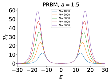
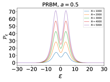
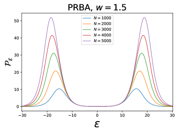
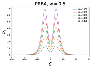
We already know the behaviour of the EE in a free fermion model with delocalized-localized phase transitionPouranvari and Yang (2014). In delocalized phase, eigenstate of the system is extended and we expect larger EE compare to the localized phase. Thus, by looking at the behavior of the EE as we change the disorder in the system, we can distinguish different phases. On the other hand, we can look at the behavior of the EE as we increase system size, $N$ with a fixed value of disorder. In delocalized phase EE increases with system size and violate the area lawEisert et al. (2010); Swingle and McGreevy (2016); Alba et al. (2019), while it saturates to a fixed value in localized phase. In addition, we can look at EE from EHS point of view. Eq. (5) tells us that among all eigenvalues of correlation function $\{\zeta\}$, those $\zeta$’s close to $1/2$ have bigger share in the EE; or in terms of EHS (see Eq. (4)), those $\epsilon$’s close to zero are the most effective spectrum in the EE, and as we move away from zero, $\epsilon$’s become less effective. So the distribution of EHS is informative.

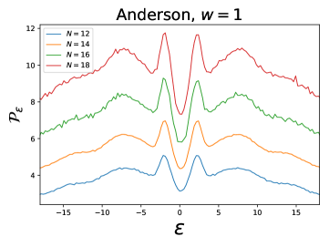
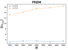
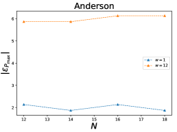
In Figs. 1, 2, and 3 we plot distribution of the EHS for PRBM, PRBA, and Anderson $3d$ models in delocalized and localized phases. We see that for each system size $N$ in the localized phase, probability distribution of $\epsilon$’s, $\mathcal{P}_{\epsilon}$, at small magnitude $\epsilon$’s is negligible and the big share comes from larger magnitude $\epsilon$’s, which according to Eq. (5) yields to low EE. In addition, as we increase system size, that $\epsilon$ corresponds to maximum probability, $\epsilon_{\mathcal{P}_{max}}$, shifts to larger magnitude (yielding to smaller EE), and the corresponding probability increases (yielding ro larger EE); i.e. two opposite factors causes EE to saturate. The behaviour of the $\epsilon$ with highest probability $\epsilon_{\mathcal{P}_{max}}$ in delocalized and localized phases as we increase system size $N$ is plotted in Fig. 4 for three mentioned models.

On the other hand, distribution of EHS for delocalized phase is noticeably different. Small values of $\epsilon$’s have big shares of probability compare to large $\epsilon$’s; which yields to a large EE. In addition, as we increase the system size, $\epsilon_{\mathcal{P}_{max}}$ stays fixed (see Fig. 4), but its probability increases. Thus, EE becomes larger as we increase system size.

Figure 1: (color online) probability distribution of the entanglement Hamiltonian spectrum for PRBM model in localized (upper panel) and delocalized (lower panel) phase. Distribution is plotted for different system sizes $N=1000,2000,3000,4000,5000$ from bottom to top. Number of samples ranges between $20000$ for small system sizes and $1000$ for large system sizes.

Figure 2: (color online) probability distribution of the entanglement Hamiltonian spectrum for PRBA model in localized (upper panel) and delocalized (lower panel) phase. Distribution is plotted for different system sizes $N=1000,2000,3000,4000,5000$ from bottom to top. Number of samples ranges between $20000$ for small system sizes and $1000$ for large system sizes.

Figure 3: (color online) probability distribution of the entanglement Hamiltonian spectrum for Anderson $3d$ model in localized (upper panel) and delocalized (lower panel) phase. Distribution is plotted for different linear system sizes $N=12,14,16,18$ from bottom to top, where system size is $N\times N\times N$. Number of samples ranges between $2000$ for small system sizes and $200$ for large system sizes.

Figure 4: (color online) behaviour of the smallest magnitude entanglement Hamiltonian eigenvalue with largest probability $\epsilon_{\mathcal{P}_{max}}$ for delocalized and localized phases in PRBM (left panel), PRBA (middle panel), and Anderson $3d$ models (right panel).

IV Smallest magnitude entanglement Hamiltonian eigenvalue

According to Figs. 1, 2 and 3, smallest magnitude $\epsilon$ has distinguishable features in delocalized and localized phases. To see it clearly, we plot the spectrum of EHS for one sample without taking disorder average in Fig. 5 for PRBM, PRBA, and Anderson $3d$ model (Since Hamiltonian of the system has randomness, we do not have particle-hole symmetry for eigenvalues of entanglement HamiltonianCheong and Henley (2004), so we do not expect a symmetric distribution of the EHS). In delocalized phase, we have a (close to) zero spectrum, while the smallest magnitude spectrum is a finite value in the localized phase.

Figure 5: (color online) spectrum of entanglement Hamiltonian for PRBM (left panel), PRBA (middle panel), and Anderson $3d$ (right panel) models in delocalized (red) and delocalized (blue) phase. For PRBM, and PRBA system size $N=100$ and for Anderson $N=6\times 6\times 6$. One sample is considered for each disorder strength without taking disorder average.

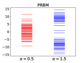
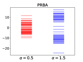
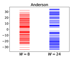
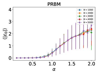
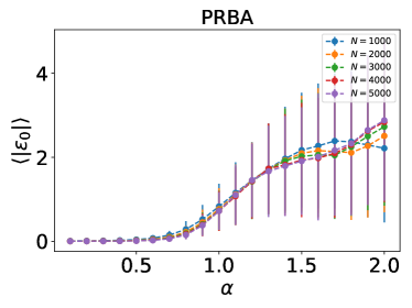
Accordingly, we propose smallest magnitude $\epsilon$ to be a characterization of the delocalized-localized phase transition. We plot disorder averaged smallest magnitude $\epsilon$ as we increase disorder strength in Fig. 6 for PRBM and PRBA models. In delocalized phase the smallest magnitude $\epsilon$ is zero, while it goes to larger $\epsilon$’s. We also note that standard deviation of disorder averaged smallest $\epsilon$ is considerably larger in the localized phase.

Figure 6: (color online) disorder averaged of smallest magnitude $\epsilon$ corresponding to non-zero probability distribution as we change disorder strength $a$ in PRBM model (upper panel), and PRBA model (lower model). In delocalized phase it is zero, and it moves toward larger values in localized phase. Vertical bar at each point shows the corresponding standard deviation.

V Conclusion

Entanglement in quantum system has been used vastly before for characterizing phases and phase transitions in condensed matter physics. EE diverges in delocalized phases and it saturates in localized phase, thus behavior of the EE as we change the disorder strength locates the phase transition point. In this report, by employing free fermion models we explained that eigenvalues of the entanglement Hamiltonian are also informative to characterize phases and the phase transition point. In addition, we explained the behavior of EE according to the distribution of the entanglement Hamiltonian eigenvalues based on which we propose a characterization for the delocalized-localized phase transition, namely the smallest magnitude entanglement Hamiltonian eigenvalue. We applied this characterization to our one dimensional models and found that its behavior is different in delocalized and localized phases, although the phase transition point is not sharply located by this characterization.