Eigenfunction asymptotics and spectral Rigidity of the ellipse

Abstract.

Microlocal defect measures for Cauchy data of Dirichlet, resp. Neumann, eigenfunctions of an ellipse $E$ are determined. We prove that, for any invariant curve for the billiard map on the boundary phase space $B^{*}E$ of an ellipse, there exists a sequence of eigenfunctions whose Cauchy data concentrates on the invariant curve. We use this result to give a new proof that ellipses are infinitesimally spectrally rigid among $C^{\infty}$ domains with the symmetries of the ellipse.

This note is part of a series [HeZe12, HeZe19] on the the inverse spectral problem for elliptical domains $E\subset{\mathbb{R}}^{2}$. In [HeZe12], it is shown, roughly speaking, that an isospectral deformation of an ellipse through smooth domains (but not necessarily real analytic) which preserves the ${\mathbb{Z}}_{2}\times{\mathbb{Z}}_{2}$ symmetry is trivial. In [HeZe19] it is shown that ellipses of small eccentricity are uniquely determined by their Dirichlet (or, Neumann) spectra among all $C^{\infty}$ domains, with no analyticity or symmetry assumptions imposed. In both [HeZe12, HeZe19], the main spectral tool is the wave trace singularity expansion and the special form it takes in the case of ellipses. In this article, we take the dual approach of studying the asymptotic concentration in the phase space $B^{*}\partial E$ of the Cauchy data $u^{b}_{j}$ of Dirichlet (or, Neumann) eigenfunctions $u_{j}$ of elliptical domains in the unit coball bundle of the boundary $\partial E$. In Theorem 1, we show that, for every regular rotation number of the billiard map in the ‘twist interval’, there exists a sequence of eigenfunctions whose Cauchy data concentrates on the invariant curve with that rotation number in $B^{*}\partial E$. The proof uses the classical separation of variables and one dimensional WKB analysis.

Before stating the results we introduce some notation and background. An orthonormal basis of Dirichlet (resp. Neumann) eigenfunctions in a bounded, smooth Euclidean plane domain $\Omega$ is denoted by

$$\left\{\begin{array}[]{l}(\Delta+\lambda_{j}^{2})\varphi_{j}=0,\;\;\langle\varphi_{j},\varphi_{k}\rangle:=\int_{\Omega}\varphi_{j}\bar{\varphi_{k}}dx,\\ \\ \varphi_{j}|_{\partial\Omega}=0,\;(\rm{resp.}\;\partial_{\nu}\varphi_{j}|_{\partial\Omega}=0),\end{array}\right.$$

where as usual $\partial_{\nu}$ denotes the inward unit normal. The semi-classcial Cauchy data is denoted by,

(1) $$u_{j}^{b}:=\left\{\begin{array}[]{ll}\varphi_{j}|_{\partial\Omega},&\mbox{Neumann}\\ &\\ \lambda_{j}^{-1}\partial_{\nu}\varphi_{j}|_{\partial\Omega},&\mbox{Dirichlet}.\end{array}\right.$$

The Cauchy data are eigenfunctions of the semi-classical eigenvalue problem, $N(\lambda_{j})u_{j}^{b}=u_{j}^{b}$, where $N(\lambda)$ is a semi-classical Fourier integral operator quantizing the billiard map $\beta:B^{*}\partial\Omega\to B^{*}\partial\Omega$ (see [HaZe04] for the precise statement).

We are interested here in the quantum limits of the Cauchy data (1) of an orthonormal basis of eigenfunctions of an ellipse, i.e. in the asymptotic limits of the matrix elements

(2) $$\rho_{j}^{b}(Op_{\hbar}(a)):=\frac{\langle Op_{\hbar}(a)u_{j}^{b},u_{j}^{b}\rangle}{\langle u_{j}^{b},u_{j}^{b}\rangle},\;\;(\hbar=\hbar_{j}=\lambda_{j}^{-1})$$

of zeroth order semi-classical pseudo-differential operators $Op_{\hbar}(a)$ on $\partial E$ with respect to the $L^{2}$-normalized Cauchy data of eigenfunctions. We note that $\rho_{j}^{b}$ is normalized so that $\rho_{j}^{b}(I)=1$ and is a positive linear functional, hence all possible weak* limits are probability measures on the unit coball bundle $B^{*}\partial\Omega$. Moreover, $\rho_{j}(N(\lambda)^{*}Op_{\hbar}(a)N(\lambda))=\rho_{j}(Op_{\hbar}(a))$, so that the quantum limits are quasi-invariant under the billiard map (see [HaZe04] for precise statements). In Theorem 1 we determine the quantum limits of sequences in (2) for an ellipse. The proof uses many of the prior results on WKB formulae for ellipse eigenfunctions, especially those of [KeRu60, WaWiDu97, Sie97].

In large part, our interest in matrix elements (2) owes to the fact that the Hadamard variational formulae for eigenvalues of the Laplacian with Dirichlet boundary condition expresses the eigenvalue variations as the special matrix elements (2) given by,

(3) $$\int_{\partial E}\dot{\rho}\;\;|u^{b}_{j}|^{2}ds$$

of the domain variation $\dot{\rho}$ (not to be confused with $\rho_{j}$) against squares of the Cauchy data (see Section 5.1). As stated in Corollary 2, the limits of such integrals over all possible subsequences of eigenfunctions determines the ‘Radon transform’ of $\dot{\rho}$ over all possible invariant curves for the billiard map. Under an infinitesimal isospectral deformation, all of the limits are zero. We use this result to give a new proof of the spectral rigidity result in [HeZe12]; see Theorem 4 and Corollary 5.

The principal motivation for studying the inverse Laplace spectral problems for ellipses stems from the Birkhoff conjecture that ellipses are the only bounded plane domains with completely integrable billiards. Strong recent results, due to A. Avila, J. de Simoi, V. Kaloshin, and A. Sorrentino [AvdSKa16, KaSo18] have proved local versions of the Birkhoff conjecture using a weaker notion of integrability known as ‘rational integrability’, i.e. that periodic orbits come in one-parameter families, namely invariant curves of the billiard map with rational rotation number. In this article, Bohr-Sommerfeld invariant curves play the principal role rather than curves of periodic orbits.

1.1. Statement of results

The first result pertains to concentration of Cauchy data of sequences $\varphi_{j}$ of Dirichlet (resp. Neumann) eigenfunctions on invariant curves of the billiard map of an ellipse. We denote $E$ by $\frac{x^{2}}{a^{2}}+\frac{y^{2}}{b^{2}}\leq 1$, $0\leq b<a$, and choose the elliptical coordinates $(\rho,\vartheta)$ by

$$(x,y)=(c\cosh\rho\cos\vartheta,c\sinh\rho\sin\vartheta).$$

Here,

$$c=\sqrt{a^{2}-b^{2}},\;\;0\leq\rho\leq\rho_{\max}=\cosh^{-1}(a/c),\;\;0\leq\vartheta\leq 2\pi.$$

We denote the angular Hamiltonian, which we will also call the action, by

$$I={p_{\vartheta}^{2}}/c^{2}+\cos^{2}\vartheta.$$

The invariant curves of $\beta$ are the level sets of $I$. The range of $I$ is called the action interval. There is a natural measure $d\mu_{\alpha}$ on each level set $I=\alpha$ called the Leray measure which is invariant under $\beta$ and the flow of $I$. We refer to Section 2 for detailed definitions and properties involving the billiard map of an ellipse, actions, invariant curves, and the Leray measure.

Theorem 1.

Let $E$ be an ellipse. For any $\alpha$ in the action interval of the billiard map of $E$, there exists a sequence of separable (in elliptical coordinates) eigenfunctions $\{\varphi_{j}\}$ of eigenvalue $\lambda_{j}^{2}$ whose Cauchy data concentrates on the level set $\{I=\alpha\}$, in the sense that, for any zeroth order semi-classical pseudo-differential operator $Op_{\hbar}(a)$ on $B^{*}\partial E$ with principal symbol $a_{0}$,

(4) $$\frac{\langle Op_{\hbar_{j}}(a)u_{j}^{b},u_{j}^{b}\rangle}{\langle u_{j}^{b},u_{j}^{b}\rangle}\to\frac{\int_{I=\alpha}a_{0}d\nu_{\alpha}}{\int_{I=\alpha}d\nu_{\alpha}},\quad(h_{j}=\lambda_{j}^{-1}\to 0)$$

where

(5) $$d\nu_{\alpha}=\left\{\begin{array}[]{ll}\frac{1}{\sqrt{c^{2}(\cosh^{2}\rho_{\max}-\cos^{2}\vartheta)}}d\mu_{\alpha},&\mbox{Dirichlet},\\ &\\ \small\sqrt{c^{2}(\cosh^{2}\rho_{\max}-\cos^{2}\vartheta)}\;d\mu_{\alpha},&\mbox{Neumann}.\end{array}\right.$$

In particular,

Corollary 2.

In the special case when the symbol $a(\vartheta,p_{\vartheta})=\dot{\rho}(\vartheta)$ is only a function of the base variable $\vartheta$,

$$\frac{\int_{\partial E}\dot{\rho}\;\;|u^{b}_{j}|^{2}ds}{\int_{\partial E}|u^{b}_{j}|^{2}ds}\to\frac{\int_{I=\alpha}\dot{\rho}\,d\nu_{\alpha}}{\int_{I=\alpha}d\nu_{\alpha}}\,,$$

where $ds=\small\sqrt{c^{2}(\cosh^{2}\rho_{\max}-\cos^{2}\vartheta)}\,d\vartheta$ is the arclength measure.

Remark 3.

If we denote $\eta$ to be the symplectic dual variable of the arclength $s$, then our quantum limit can be expressed as

$$d\nu_{\alpha}=\left\{\begin{array}[]{ll}\sqrt{1-|\eta|^{2}}\,d\mu_{\alpha},&\mbox{Dirichlet},\\ &\\ \small\frac{1}{\sqrt{1-|\eta|^{2}}}\;d\mu_{\alpha},&\mbox{Neumann}.\end{array}\right.$$

For the proof, see our computation of ${1-|\eta|^{2}}$ in the proof of Corollary 18.

The appearance of the (non-invariant) factors $\sqrt{1-|\eta|^{2}}$ and $1/\sqrt{1-|\eta|^{2}}$ is consistent with the result of [HaZe04], where the quantum limits of boundary traces of ergodic billiard tables are studied.

To our knowledge, Theorem 1 is the first result on microlocal defect measures of Cauchy data of eigenfunctions in non-ergodic cases. See Section 1.3 for related results. One of the difficulties in determining the limits of (2) is that the Cauchy data $u_{j}^{b}$ are not $L^{2}$ normalized. It is shown in [HaTa02, Theorem 1.1] that there exists $C,c>0$ so that

$$c\leq||\lambda_{j}^{-1}\partial_{\nu}\varphi_{j}||_{L^{2}(\partial\Omega)}\leq C$$

for Dirichlet eigenfunctions of Euclidean plane domains (and more general non-trapping cases). Hence the $L^{2}$ normalization in (2) is rather mild. On the other hand, the corresponding inequalities do not hold in general for Neumann eigenfunctions. As pointed out in [HaTa02, Example 7], there are simple counter-examples to any constant upper bound on the unit disc (whispering gallery modes). There do exist positive lower bounds for convex Euclidean domains. Hence, in the case of an ellipse, the $L^{2}$ normalization in (2) is necessary to obtain limits.

1.2. Spectral rigidity

Before stating the results, we review the main definitions. An isospectral deformation of a plane domain $\Omega_{0}$ is a one-parameter family $\Omega_{t}$ of plane domains for which the spectrum of the Euclidean Dirichlet (or Neumann, or Robin) Laplacian $\Delta_{t}$ is constant (including multiplicities). The deformation is said to be a $C^{1}$ deformation through $C^{\infty}$ domains if each $\Omega_{t}$ is a $C^{\infty}$ domain and the map $t\to\Omega_{t}$ is $C^{1}$. We parameterize the boundary $\partial\Omega_{t}$ as the image under the map

(6) $$x\in\partial\Omega_{0}\to x+\rho_{t}(x)\nu_{x},$$

where $\rho_{t}\in C^{1}([0,t_{0}],C^{\infty}(\partial\Omega))$. The first variation is defined to be $\dot{\rho}(x):=\frac{d}{dt}{|_{t=0}}\rho_{t}(x)$. An isospectral deformation is said to be trivial if $\Omega_{t}=\Omega_{0}$ (up to isometry) for sufficiently small $t$. A domain $\Omega_{0}$ is said to be spectrally rigid if all $C^{\infty}$ isospectral deformations are trivial.

In [HeZe12] the authors proved a somewhat weaker form of spectral rigidity for ellipses, with ‘flatness’ replacing ‘triviality’. Its main result is the infinitesimal spectral rigidity of ellipses among $C^{\infty}$ plane domains with the symmetries of an ellipse. We orient the domains so that the symmetry axes are the $x$-$y$ axes. The symmetry assumption is then that $\rho_{t}$ is invariant under $(x,y)\to(\pm x,\pm y)$. The variation is called infinitesimally spectrally rigid if $\dot{\rho}_{0}=0$.

The main result of [HeZe12] is:

Theorem 4.

Suppose that $\Omega_{0}$ is an ellipse, and that $\Omega_{t}$ is a $C^{1}$ Dirichlet (or Neumann) isospectral deformation of $\Omega_{0}$ through $C^{\infty}$ domains with ${\mathbb{Z}}_{2}\times{\mathbb{Z}}_{2}$ symmetry. Let $\rho_{t}$ be as in (6). Then $\dot{\rho}=0$.

Corollary 5.

Suppose that $\Omega_{0}$ is an ellipse, and that $t\to\Omega_{t}$ is a $C^{1}$ Dirichlet (or Neumann) isospectral deformation through ${\mathbb{Z}}_{2}\times{\mathbb{Z}}_{2}$ symmetric $C^{\infty}$ domains. Then $\rho_{t}$ must be flat at $t=0$.

The proof of Theorem 4 in [HeZe12] used the variation of the wave trace. In the original posting (arXiv:1007.1741) the authors used a more classical Hadamard variational formula for variations of individual eigenvalues $\lambda_{j}(t)$, which appears in Section 5.1. The authors rejected this approach in favor of the one appearing in [HeZe12] because it was thought that this argument was invalid when the eigenvalues were multiple. When a multiple eigenvalue of a 1-parameter family $L_{t}$ of operators is perturbed, it splits into a collection of branches which in general are not differentiable in $t$. Moreover, the authors assumed that the variational formula would express the variation in terms of special separable eigenfunctions (see Section 3). This created doubt that one could use the variational formula for individual eigenvalues. Instead, the authors used the variational formula for the trace of the wave group or equivalently for spectral projections, which are symmetric sums over all of the branches into which an eigenvalue splits.

However, as we show in this article, the original variational formulae were in fact correct even in the presence of multiplicities. The first point is that the non-differentiability issue does not arise for an isospectral deformation since no splitting occurs. Second, the vanishing of the variation of eigenvalues implies that the infinitesimal variation $\dot{\rho}$ is orthogonal to squares of all (Dirichlet) eigenfunctions in the eigenspace, and in particular the separable ones. More precisely, we prove that

$$\int_{\partial E}\dot{\rho}\;\;|u^{b}_{j}|^{2}ds=0.$$

Then by Corollary 5, we obtain that for every $\alpha$ in the action interval one has

(7) $$\int_{I=\alpha}\dot{\rho}\,d\nu_{\alpha}=0.$$

In the final step we calculate the measure $d\nu_{\alpha}$ and provide two proofs, one via inverting an Abel transform and another using the Stone-Weierstrass theorem, that (7) implies $\dot{\rho}=0$. The proof in the Neumann case is similar and will be provided.

1.3. Related results and open problems

Quantum limits of Cauchy data on manifolds with boundary have been studied in [HaZe04, ChToZe13] in the case where the billiard map $\beta$ is ergodic. To our knowledge, they have not been studied before in non-ergodic cases. Theorem 1 shows that, as expected, Cauchy data of eigenfunctions localize on invariant curves for the billiard map rather than delocalize as in ergodic cases.

$L^{2}$ norms of Cauchy data of eigenfunctions are studied in [HaTa02] in the Dirichlet case and in [BaHaTa18] in the Neumann case. Further results on the quasi-orthonormality properties of Cauchy are studied in [BFSS02, HHHZ15].

The study of eigenfunctions in ellipses has a long literature and we make substantial use of it. In particular, we quote several articles in the physics literature, in particular [WaWiDu97, Sie97], and several in mathematics [KeRu60, BaBu91], for detailed analyses of eigenfunctions of the quantum ellipse. There is also a series of articles of G. Popov and P. Topalov (see e.g. [PoTo03, PT16]) on the use of KAM quasi-modes to study Laplace inverse spectral problems. In particular, in [PT16], Popov-Topalov also give a new proof of the rigidity result of [HeZe12] and extend it to other settings. The approach in this article is closely related to theirs, although it does not seem that the authors directly studied Cauchy data of eigenfunctions of an ellipse.

The multiplicity of Laplace eigenvalues of an ellipse appears to be largely an open problem. It is a non-trivial result of C.L. Siegel that the multiplicities are either $1$ or $2$ in the case of circular billiards; multiplicity $1$ occurs for, and only for, rotationally invariant eigenfunctions. The Laplacians of the family of ellipses $\frac{x^{2}}{a^{2}}+\frac{y^{2}}{b^{2}}=1$ form an analytic family containing the disk Laplacian, and one might try to use analytic perturbation theory to prove the following,

Conjecture 6.

For a generic class of ellipses the multiplicity of each eigenvalue is $\leq 2$.

1.4. Quantum Birkhoff conjecture

As mentioned above, ellipses have completely integrable billiards, and the classical Birkhoff conjecture is that elliptical billiards are the only completely integrable Euclidean billiards with convex bounded smooth domains. Despite much recent progress, the Birkhoff conjecture remains open.

The eigenvalue problem on a Euclidean domain is often called ‘quantum billiards’ in the physics literature (see e.g. [WaWiDu97]). One could formulate quantum analogues of the Birkhoff conjecture in several related but different ways. The quantum analogue of the Birkhoff conjecture is presumably that ellipses are the only ‘quantum integrable’ billiard tables. A standard notion of quantum integrability is that the Laplacian commutes with a second, independent, (pseudo-differential) operator; we refer to [ToZe03] for background on quantum integrability. In Section 3, we explain that the ellipse is quantum integrable in that one may construct two commuting Schrödinger operators with the same eigenfunctions and eigenvalues. The symbol of the second operator then Poisson commutes with the symbol of the Laplacian, hence the billiard dynamics and billiard map are integrable. A related version is that one can separate variables in solving the Laplace eigenvalue problem. It is not obvious that these two notions are equivalent; in Section 3 we use both separation of variables and existence of commuting operators in studying the ellipse. Classical studies of separation of variables and its relation to integrability go back to C. Jacobi, P. Stäckel, L. Eisenhart and others, and E.K. Sklyanin has studied the problem more recently. We do not make use of their results here.

Quantum integrability is much stronger than classical integrability, and one might guess that it is simpler to prove the quantum Birkhoff conjecture than the classical one. Wave trace techniques as in [HeZe12, HeZe19] reduce Laplace spectral determination and rigidity problems to dynamical inverse or rigidity results. The wave trace only ‘sees’ periodic orbits and is therefore well-adapted to results on rational integrability. The dual approach through eigenfunctions studied in this article gives a different path to the quantum Birkhoff conjecture, in which rational integrability and periodic orbits play no role.

2. Classical billiard dynamics

In this, and the next, section, we review some background definitions and results on the classical and quantum elliptical billiard. We follow the notation of [Sie97]; see also [BaBu91, WaWiDu97].

An ellipse $E$ is a plane domain defined by,

$$\frac{x^{2}}{a^{2}}+\frac{y^{2}}{b^{2}}\leq 1,\;\;\;0\leq b<a.$$

Here, $a,$ resp. $b$, is the length of the semi-major (resp. semi-minor) axis. The ellipse has foci at $(\pm c,0)$ with $c=\sqrt{a^{2}-b^{2}}$ and its eccentricity is $e=\frac{c}{a}$. Its area is $\pi ab$, which is fixed under an isospectral deformation. We define elliptical coordinates $(\rho,\vartheta)$ by

$$(x,y)=(c\cosh\rho\cos\vartheta,c\sinh\rho\sin\vartheta).$$

Here,

$$0\leq\rho\leq\rho_{\max}=\cosh^{-1}(a/c),\;\;0\leq\vartheta\leq 2\pi.$$

The coordinates are orthogonal. The lines $\rho={constant}$ are confocal ellipses and the lines $\vartheta={constant}$ are confocal hyperbolas. In the special case of the disc, we have $c=0$, but we assume henceforth that $c\not=0$.

2.1. Action variables for the billiard flow

The billiard flow on the ellipse $E$ is the (broken) geodesic flow of the Hamiltonian $H={p_{x}^{2}+p_{y}^{2}}$ on $T^{*}E$, which follows straight lines inside $E$ and reflects on $\partial E$ according to equal angle law of reflection.

Action-angle variables on $T^{*}E$ are symplectic coordinates in which the billiard flow of the ellipse is given by Kronecker flows on the invariant Lagrangian submanifolds. We refer to [Ar89] for the general principles and to [Sie97] for the special case of the ellipse. Let $p_{\rho}$ and $p_{\vartheta}$ be the symplectic dual variables corresponding to the elliptic coordinates $\rho$ and $\vartheta$, respectively. The two conserved quantities of the system are the energy (the Hamiltonian) $H$ and the angular Hamiltonian $I$ (which we also call the action), given in the coordinates $(\rho,p_{\rho},\vartheta,p_{\vartheta})$, by

$$H=\frac{p_{\rho}^{2}+p_{\vartheta}^{2}}{c^{2}(\cosh^{2}\rho-\cos^{2}\vartheta)}\quad\text{and}\quad I=\frac{p_{\vartheta}^{2}\cosh^{2}\rho+p_{\rho}^{2}\cos^{2}\vartheta}{p_{\rho}^{2}+p_{\vartheta}^{2}}.$$

In the notation of [Tab97],

$$I=\cos^{2}\theta\cosh^{2}\rho+\sin^{2}\theta\cos^{2}\vartheta,$$

where $\theta$ is the angle between a trajectory of the billiard flow and a tangent vector to the confocal ellipse with parameter $\rho$. Note also that by the notation of [Sie97], $I=1+\frac{L_{1}L_{2}}{c^{2}H}$ where $L_{1}L_{2}$ is the product of two angular momenta about the two foci. The values of $I$ are restricted to

$$0\leq I\leq\frac{a^{2}}{c^{2}}=\cosh^{2}(\rho_{\text{max}}).$$

The upper limit $I=\cosh^{2}(\rho_{\text{max}})$ corresponds to the motion along the boundary and the lower limit $I=0$ corresponds to the motion along the minor axis. Moreover, there are two different kinds of motion in the ellipse depending on the sign of $I$. For $1<I<\cosh^{2}(\rho_{\text{max}})$ the trajectories have a caustic in the form of a confocal ellipse. For $0<I<1$ the caustic of the motion is a confocal hyperbola and the trajectories cross the $x$-axis between the two focal points. Both kinds of motions are separated by a separatrix which consists of orbits with $I=1$ that go through the focal points of the ellipse.

In terms of $H$ and $I$, the canonical momenta, are given by

(8) $$p_{\rho}^{2}=c^{2}(\cosh^{2}\rho-I)H\quad\text{and}\quad p_{\vartheta}^{2}=c^{2}(I-\cos^{2}\vartheta)H.$$

Therefore, the action variables are

(9) $$I_{\rho} =\frac{1}{2\pi}\int p_{\rho}\,d\rho=\frac{c\sqrt{H}}{\pi}\int_{\cosh^{2}\rho\geq I,\rho\geq 0}\sqrt{\cosh^{2}\rho-I}\,d\rho,$$

(10) $$I_{\vartheta} =\frac{1}{2\pi}\int p_{\vartheta}\,d\vartheta=\frac{c\sqrt{H}}{\pi}\int_{\cos^{2}\vartheta\leq I,0\leq\varphi\leq\pi}\sqrt{I-\cos^{2}\vartheta}\,d\vartheta.$$

In fact these are the actions for the half-ellipse $0\leq\varphi\leq\pi$. The integrals can be calculated in terms of $I$ using elliptic integrals of first and second kind (See [Sie97]). The actions will play a key role in Section 3.4 in the description of Bohr-Sommerfeld quantization conditions for the eigenvalues of the Laplacian.

(a)

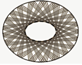
(b)

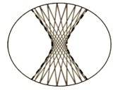
(c)

Figure 1. Invariant curves and caustics.

2.2. Billiard map, invariant curves, Leray measure, and action-angle variables

The billiard map of an ellipse $E$ (or in general any smooth domain) is a cross section to the the billiard flow on $S^{*}_{\partial E}E$, which we always identify with $B^{*}\partial E$ and call it the phase space of the boundary. To be precise, the billiard map $\beta$ is defined on $B^{*}\partial E$ as follows: given $(s,\eta)\in T^{*}\partial E$, with $s$ being the arc-length variable measured in the counter-clockwise direction from a fixed point say $s_{0}$, and $|\eta|\leq 1$, we let $(s,\zeta)\in S^{*}E$ be the unique inward-pointing unit covector at $s$ which projects to $(s,\eta)$ under the map $T^{*}_{\partial E}E\to T^{*}\partial E$. Then we follow the geodesic (straight line) determined by $(s,\zeta)$ to the first place it intersects the boundary again; let $s^{\prime}\in\partial E$ denote this first intersection. (If $|\eta|=1$, then we let $s^{\prime}=s$.) Denoting the inward unit normal vector at $s^{\prime}$ by $\nu_{s^{\prime}}$, we let $\zeta^{\prime}=\zeta+2(\zeta\cdot\nu_{s^{\prime}})\nu_{s^{\prime}}$ be the direction of the geodesic after elastic reflection at $s^{\prime}$, and let $\eta^{\prime}$ be the projection of $\zeta^{\prime}$ to $T^{*}_{s^{\prime}}Y$. Then we define

$$\beta(s,\eta)=(s^{\prime},\eta^{\prime}).$$

A theorem of Birkhoff asserts that billiard map preserves the natural symplectic form $ds\wedge d\eta$ on $B^{*}\partial E$, i.e.

$$\beta^{*}(ds\wedge d\eta)=ds\wedge d\eta.$$

In the literature, the coordinates $(s,\theta)$ are commonly used for phase space of the boundary, where $\theta\in[0,\pi]$ is the angle that $\zeta$ makes with the positive tangent direction at $s$. In these coordinates,

$$ds\wedge d\eta=\sin\theta\,d\theta\wedge ds$$

An invariant set in $B^{*}\partial E$ is a set $C$ such that $\beta(C)=C$. An invariant curve is a curve (connected or not) on the phase space that is invariant. The phase space $B^{*}\partial E$ of the ellipse $E$ is in fact foliated with invariant curves. More precisely,

Lemma 7.

The invariant curves of the billiard map $\beta:B^{*}\partial E\to B^{*}\partial E$ are level sets of $I:B^{*}\partial E\to{\mathbb{R}}$ defined by,

$$I=\frac{p_{\vartheta}^{2}}{c^{2}}+\cos^{2}\vartheta$$

Proof.

It follows quickly form the second equation of (8) and that $H=1$ on $S^{*}\partial E$. ∎

Although $I_{\vartheta}$ is the classical angular action on $B^{*}\partial E$, but we shall call $I$ the action as it is more convenient and is related to $I_{\vartheta}$ via the one-to-one correspondence (10). As is evident from the Figure 1, the separatrix curve $I=1$ divides the phase space into two types of open sets, the exterior corresponding to trajectories with confocal elliptical caustics ($1<I<\cosh^{2}\rho_{\text{max}}$) and the interior to trajectories with confocal hyperbolic caustics ($0<I<1$).

2.2.1. Leray measure

On each level set $I=\alpha$ of $I$, there is a natural measure $d\mu_{\alpha}$ called the Leray measure which in invariant under $\beta$ and the flow generated by $I$. In the symplectic coordinates $(\vartheta,p_{\vartheta})$, and on $I=\alpha$, it is given by

$$d\mu_{\alpha}=\frac{d\vartheta\wedge dp_{\vartheta}}{dI}.$$

Since $d\vartheta\wedge dI=\frac{\partial I}{\partial p_{\vartheta}}d\vartheta\wedge dp_{\vartheta}$, we obtain that

(11) $$d\mu_{\alpha}=\frac{c^{2}}{2p_{\vartheta}}\bigg{\rvert}_{I=\alpha}d\vartheta=\frac{c}{2}(\alpha-\cos^{2}\vartheta)_{+}^{-1/2}d\vartheta.$$

Here, $x_{+}=x$ if $x>0$ and is zero otherwise. Up to a scalar multiplication, $d\mu_{\alpha}$ is a unique measure that is invariant under $\beta$ and the flow of $I$.

2.2.2. Action-angle variables and rotation number

The billiard map has a Birkhoff normal form around each invariant curve in $B^{*}\partial E$. That is, in the symplectically dual angle variable $\iota$ to $I$, the billiard map has the form, $\beta(I,\iota)=(I,\iota+r(I))$, where $r$ is often called the rotation number of the invariant curve. An explicit formula is given for it in [Tab97] (3.5), [CaRa10] (section 4.3 (11)) and [Ko85]. Then, if $0<I<1$,

$$r(I)=\frac{\pi}{2F(\sqrt{I})}F\left(\arcsin\left(\frac{2\tanh(\rho_{\text{max}})\sqrt{\cosh^{2}\rho_{\text{max}}-I}}{\cosh^{2}\rho_{\text{max}}-I+I\tanh^{2}\rho_{\text{max}}}\right),\sqrt{I}\right),$$

where

$$F(z,k)=\int_{0}^{z}\frac{d\tau}{\sqrt{1-k^{2}\sin^{2}\tau}},\;\;F(k)=F\left(\frac{\pi}{2},k\right).$$

Also, if $1<I<\cosh^{2}(\rho_{\text{max}})$ then

$$r(I)=\frac{\pi}{2F(1/\sqrt{I})}F\left(\arcsin\left(\sqrt{I}\frac{2\tanh(\rho_{\text{max}})\sqrt{\cosh^{2}\rho_{\text{max}}-I}}{\cosh^{2}\rho_{\text{max}}-I+I\tanh^{2}\rho_{\text{max}}}\right),\frac{1}{\sqrt{I}}\right).$$

Definition: We define the range of the action variable $I$ as the action interval, i.e. the interval $[0,\cosh^{2}(\rho_{\text{max}})]$, and the range of $r(I)$ as the rotation interval.

3. Quantum elliptical billiard

The Helmholtz equation in elliptical coordinates takes the form,

(12) $$-\left(\frac{\partial^{2}}{\partial\rho^{2}}+\frac{\partial^{2}}{\partial\vartheta^{2}}\right)\varphi=\lambda^{2}c^{2}(\cosh^{2}\rho-\cos^{2}\vartheta)\varphi.$$

The quantum integrability of $\Delta$ owes to the fact that this equation is separable. We put

(13) $$\varphi(\rho,\vartheta)=F(\rho)G(\vartheta),$$

and separate variables to get the coupled Mathieu equations,

(14) $$\left\{\begin{array}[]{ll}\frac{{\hbar^{2}}}{c^{2}}\,F^{\prime\prime}(\rho)+\cosh^{2}\rho\,F(\rho)=\alpha F(\rho)&\rm{DBC}\;(\rm{resp.}\,NBC),\\ &\\ -\frac{\hbar^{2}}{c^{2}}\,G^{\prime\prime}(\vartheta)+\cos^{2}\vartheta\,G(\vartheta)=\alpha G(\vartheta)&\rm{PBC}.\end{array}\right.$$

where $\hbar=\lambda^{-1}$ and $\alpha$ is the separation constant. Here, ‘PBC’ stands for ‘periodic boundary conditions’; DBC (resp. NBC) stands for Dirichlet (resp. Neumann) boundary conditions. Thus, we consider pairs $(\hbar,\alpha)$ where there exists a smooth solution of the two boundary problems.

Each of the angular and radial equations above is an eigenvalue problem for a semiclassical Schrödinger operator with boundary conditions on a finite interval. These commuting operators are given by

(15) $$Op_{\hbar}(J);\quad J =-{p_{\rho}^{2}}/{c^{2}}+\cosh^{2}(\rho),$$

(16) $$Op_{\hbar}(I);\quad I ={p_{\vartheta}^{2}}/{c^{2}}+\cos^{2}(\vartheta).$$

The boundary conditions on $F$ take the form,

(17) $$\;\;F(\rho_{\max})=0\;\;\;\;(\mbox{Dirichlet}),\;\;\;F^{\prime}(\rho_{\max})=0\;\;\;(\mbox{Neumann}).$$

As $G(-\vartheta)$ is a solution whenever $G(\vartheta)$ is, we restrict our attention to $2\pi$-periodic solutions to the angular equation which are either even or odd. One can then see that:

Remark 8.

In order to obtain solutions well-defined on the line segment joining the foci, i.e. at $\rho=0$, solutions to the radial equation must satisfy the boundary condition $F^{\prime}(0)=0$ in case the solution $G$ is even and $F(0)=0$ in case $G$ is odd. In these cases the solutions $F$ are also respectively even and odd functions.

3.1. Mathieu and modified Mathieu characteristic numbers

For each fixed $\hbar$, the angular problem is a Sturm-Liouville problem and thus there exist real valued sequences $\{a^{\prime}_{n}(\hbar)\}_{n=0}^{\infty}$ and $\{b^{\prime}_{n}(\hbar)\}_{n=1}^{\infty}$ so that it has $2\pi$-periodic non-trivial solutions - even solutions if $\alpha=a_{n}(\hbar)$ and odd solutions if $\alpha=b_{n}(\hbar)$. Here even or odd is with respect to $\vartheta\to-\vartheta$, or equivalently $y\to-y$. We represent the corresponding solutions by $G_{n}^{\text{e}}(\vartheta,\hbar)$ and $G_{n}^{\text{o}}(\vartheta,\hbar)$, respectively. The even indices correspond to $\pi$-periodic solutions, thus they must be invariant under $\vartheta\to\pi-\vartheta$, or equivalently be even with respect to $x\to-x$. Solutions with odd indices have anti-period $\pi$ and correspond to odd solutions in the $x$ variable. The sequences $a^{\prime}_{n}(\hbar)$ and $b^{\prime}_{n}(\hbar)$ are related to the standard Mathieu characteristic numbers of integer orders $a_{n}(q)$ and $b_{n}(q)$ by

(18) $$a^{\prime}_{n}(\hbar)=\frac{1}{2}+\frac{a_{n}(q)}{4q},\quad b^{\prime}_{n}(\hbar)=\frac{1}{2}+\frac{b_{n}(q)}{4q},\quad q=\frac{c^{2}}{4\hbar^{2}}.$$

Thus using the wellknown properties of $a_{n}$ and $b_{n}$, for $\hbar>0$ we have

(19) $$a^{\prime}_{0}(\hbar)<b^{\prime}_{1}(\hbar)<a^{\prime}_{1}(\hbar)<b^{\prime}_{2}(\hbar)<a^{\prime}_{2}(\hbar)<b^{\prime}_{3}(\hbar)<\cdots,$$

(20) $$b^{\prime}_{n+1}(\hbar)-a^{\prime}_{n}(\hbar)={\mathcal{O}}_{n}(e^{-C/\hbar}),\quad C>0.$$

The sequence (19) is precisely the spectrum of the angular Schrödinger operator on the flat circle ${\mathbb{R}}/(2\pi{\mathbb{Z}})$.

Similarly for the radial problem (say with Dirichlet boundary condition $F(\rho_{\max})=0$), for each $\hbar$, there exist sequences $\{A^{\prime}_{m}(\hbar)\}_{m=0}^{\infty}$ and $\{B^{\prime}_{m}(\hbar)\}_{m=1}^{\infty}$ such that the radial problem has a non-trivial even solution $F_{m}^{\text{e}}(\rho,\hbar)$ if $\alpha=A^{\prime}_{m}(\hbar)$, and a odd solution $F_{m}^{\text{o}}(\rho,\hbar)$ if $\alpha=B^{\prime}_{m}(\hbar)$. The sequences of $A^{\prime}_{m}(\hbar)$ and $B^{\prime}_{m}(\hbar)$ are related to modified Mathieu characteristic numbers $A_{m}(q)$ and $B_{m}(q)$ (See [Ne10]) by the same relations as in (18). They form the spectrum of the radial semiclassical Schrödinger operator on the interval $[-\rho_{\text{max}},\rho_{\text{max}}]$ with Dirichlet boundary condition and satisfy

(21) $$A^{\prime}_{0}(\hbar)<B^{\prime}_{1}(\hbar)<A^{\prime}_{1}(\hbar)<B^{\prime}_{2}(\hbar)<A^{\prime}_{2}(\hbar)<B^{\prime}_{3}(\hbar)<\cdots.$$

3.2. Eigevalues of $E$: Intersection of Mathieu and modified Mathieu curves

In order to find eigenfunctions of the ellipse $E$ one has to search specific values of $\hbar$ such that both radial and angular Sturm-Liouville problems possess non-trivial solutions for the same value of $\alpha$. By Remark 8, we only consider the separable solutions

$$F_{m}^{\text{e}}(\rho,\hbar)G_{n}^{\text{e}}(\vartheta,\hbar)\quad\text{and}\quad F_{m}^{\text{o}}(\rho,\hbar)G_{n}^{\text{o}}(\vartheta,\hbar).$$

Thus the frequencies of $E$ with Dirichlet boundary condition are of the form

$$\lambda_{mn}^{\text{e}}=\frac{1}{\hbar_{mn}^{\text{e}}}\quad\text{and}\quad\lambda_{mn}^{\text{o}}=\frac{1}{\hbar_{mn}^{\text{o}}},$$

where $\hbar_{mn}^{\text{e}}$ and $\hbar_{mn}^{\text{o}}$ are, respectively, solutions to

(22) $$a^{\prime}_{n}(\hbar)=A^{\prime}_{m}(\hbar)\quad\text{and}\quad b^{\prime}_{n}(\hbar)=B^{\prime}_{m}(\hbar).$$

The existence of the point of intersection of the curves $a^{\prime}_{n}(\hbar)$ with $A^{\prime}_{m}(\hbar)$, and $b^{\prime}_{n}(\hbar)$ with $B^{\prime}_{m}(\hbar)$ are guaranteed by:

Theorem 9 (Neves [Ne10]).

For each $(m,n)$, there is a unique positive solution $q$ to each of the equations $a_{n}(q)=A_{m}(q)$ and $b_{n}(q)=B_{m}(q)$.

Hence the same statement holds for the equations (22) by the correspondence $\eqref{aa'relation}$. The frequencies $\lambda_{j}$ of $E$ are obtained by sorting $\{\lambda_{mn}^{\text{e}},\lambda_{mn}^{\text{o}};(m,n)\in\mathbb{N}^{2}\}$ in increasing order.

3.3. Symmetries classes

The irreducible representations of the ${\mathbb{Z}}_{2}\times{\mathbb{Z}}_{2}$ symmetry group are real one-dimensional spaces, so that there exists an orthonormal basis of eigenfunctions of the ellipse which are even or odd with respect to each ${\mathbb{Z}}_{2}$ symmetry, i.e. have one of the four symmetries

$$(\rm{even},\rm{even}),(\rm{even},\rm{odd}),(\rm{odd},\rm{even}),(\rm{odd},\rm{odd}),$$

where the first and the second entries correspond to symmetries with respect to $x\to-x$ and $y\to-y$, respectively. Given the above discussion the symmetric eigenfunctions are:

(23) $$\left\{\begin{array}[]{llll}(\rm{even},\rm{even}):&\varphi_{m,2k}^{\text{e}}&=F^{\text{e}}_{m}(\rho,\hbar)G^{\text{e}}_{2k}(\vartheta,\hbar);&\hbar=\hbar_{m,2k}^{\text{e}},\\ \\ (\rm{even},\rm{odd}):&\varphi_{m,2k}^{\text{o}}&=F^{\text{o}}_{m}(\rho,\hbar)G^{\text{o}}_{2k}(\vartheta,\hbar);&\hbar=\hbar_{m,2k}^{\text{o}},\\ \\ (\rm{odd},\rm{even}):&\varphi_{m,2k+1}^{\text{e}}&=F^{\text{e}}_{m}(\rho,\hbar)G^{\text{e}}_{2k+1}(\vartheta,\hbar);&\hbar=\hbar_{m,2k+1}^{\text{e}},\\ \\ (\rm{odd},\rm{odd}):&\varphi_{m,2k+1}^{\text{o}}&=F^{\text{o}}_{m}(\rho,\hbar)G^{\text{o}}_{2k+1}(\vartheta,\hbar);&\hbar=\hbar_{m,2k+1}^{\text{o}}.\end{array}\right.$$

\begin{overpic}[width=234.87749pt,tics=10]{EllipseSymmetries.jpg} \put(5.0,40.0){\small even in $x$, even in $y$} \put(60.0,40.0){\small odd in $x$, even in $y$} \put(5.0,-2.0){\small even in $x$, odd in $y$} \put(60.0,-2.0){\small odd in $x$, odd in $y$} \end{overpic}

Figure 2. Symmetries classes of Dirichlet eigenfunctions corresponding to the first four eigenvalues, shown by their probability densities.

Figure 2 shows the symmetries classes of eigenfunctions distinguished by their probability densities. It is possible that two symmetric eigenfunctions correspond to the same eigenvalue, or it is possible that they correspond to different eigenvalues.

3.4. Semiclassical actions and Bohr-Sommerfeld quantization conditions for the ellipse

Graphs of the one-dimensional classical potentials are given in [WaWiDu97, Figure 1]. The potential $-\cosh^{2}\rho$ for $Op_{\hbar}(J)$ in (15) is a potential barrier with a single local maximim which is symmetric around the vertical line through the local maximum. The classical potential $\cos^{2}\vartheta$ underlying $Op_{\hbar}(I)$ in (16) is a double-well potential on the circle. Thus, there exists a separatrix curve corresponding to the two local maxima of the potential, which divides the two-dimensional phase space into two regions. Inside the phase space curve, the level sets of the potential are ‘circles’ paired by the left right symmetry across the vertical line through the local maximum at $\pi$. Outside the separatrix, the level sets have non-singular projections to the base, i.e. are roughly horizontal.

As will be seen below, the Bohr-Sommerfeld levels inside the separatrix are invariant under the up-down symmetry and have two components exchanged by the left-right symmetry. The levels outside the separatrix are invariant under the left-right symmetry and are exchanged under the up-down symmetry.

It is more important for our purposes to determine the lattice of semi-classical eigenvalues in terms of classical and quantum action variables. The WKB (or EKB) quantization for the actions are given in [Sie97, (33)] (see also [KeRu60] for the original reference). Up to $\mathcal{O}(\hbar^{2})$ terms they have the form:

$$\text{Odd in $y$}\,\begin{cases}\begin{array}[]{lllll}I>1:&I_{\rho}=(m+\frac{3}{4})\hbar,&I_{\vartheta}=(n+1)\hbar,&m,n=0,1,2,\dots,\\ &&&&\\ I<1:&I_{\rho}=(m+1)\hbar,&I_{\vartheta}=(n+{\frac{1}{2}})\hbar,&m,n=0,1,2,\dots,\end{array}\end{cases}$$

$$\text{Even in $y$}\,\begin{cases}\begin{array}[]{lllll}I>1:&I_{\rho}=(m+\frac{3}{4})\hbar,&I_{\vartheta}=n\hbar,&m,n=0,1,2,\dots,\\ &&&&\\ I<1:&I_{\rho}=(m+{\frac{1}{2}})\hbar,&I_{\vartheta}=(n+{\frac{1}{2}})\hbar,&m,n=0,1,2,\dots.\end{array}\end{cases}$$

There is a discontinuity at $I=1$ due to the separatrix curve, but it is not important for our problem and we ignore it.

3.4.1. Semiclassical action

In fact for each of the eight Bohr-Sommerfeld quantization condition above there is a version which is valid to all orders in $\hbar$ which are essentially given by the quantum Birkhoff normal form around each orbit under consideration. To be precise, there exist eight so called semiclassical actions

$$S_{\hbar}^{e/o,1^{\pm},\rho/\vartheta}(\alpha),$$

where the choices of $e/o$ corresponds to even or odd in the $y$ (equivalently in the $\vartheta$) variable, of $1^{+}$ or $1^{-}$ to $I>1$ or $I<1$, and $\rho$ or $\vartheta$ to actions in the $\rho$ or $\vartheta$ variable, respectively. Each of the eight semiclassical actions has an $\hbar$ asymptotic expansion of the form

$$S_{\hbar}(\alpha)=S_{0}(\alpha)+\hbar S_{1}(\alpha)+\hbar^{2}S_{2}(\alpha)+\cdots,$$

where $S_{0}(\alpha)$ is the corresponding classical action which is $I_{\rho}|_{I=\alpha}$ for $S^{e/o,1^{\pm},\rho}_{\hbar}$ and $I_{\vartheta}|_{I=\alpha}$ for $S_{\hbar}^{e/o,1^{\pm},\vartheta}$. See equations (10) and (9) for formulas for the classical actions in terms of $I=\alpha$. Then the Bohr-Sommerfeld Quantization Conditions (BSQC) to all orders are given by

(24) $$S_{\hbar}^{e/o,1^{+},\rho}(\alpha^{e/o,1^{+},\rho}_{m}(\hbar)) =m\hbar,\quad \text{valid uniformly for $\alpha\in[1+\epsilon,\cosh^{2}{\rho_{\max}}-\epsilon]$},$$

(25) $$S_{\hbar}^{e/o,1^{+},\vartheta}(\alpha^{e/o,1^{+},\vartheta}_{n}(\hbar)) =n\hbar,\quad \alpha\in[1+\epsilon,\cosh^{2}{\rho_{\max}}-\epsilon]$$ valid uniformly for

(26) $$S_{\hbar}^{e/o,1^{-},\rho}(\alpha^{e/o,1^{-},\rho}_{m}(\hbar)) =m\hbar,\quad \text{valid uniformly for $\alpha\in[\epsilon,1-\epsilon]$},$$

(27) $$S_{\hbar}^{e/o,1^{-},\vartheta}(\alpha^{e/o,1^{-},\vartheta}_{n}(\hbar)) =n\hbar,\quad \text{valid uniformly for $\alpha\in[\epsilon,1-\epsilon]$},$$

where $\epsilon>0$ is arbitrary, however the remainder estimates in the asymptotic expansions depend on $\epsilon$. There are versions of BSQC in the literature that are valid uniformly near the separatrix but we do not need it here. We also point out that the Maslov indices are not ignored but absorbed in the corresponding subleading terms $S_{1}(\alpha)$.

Remark 10.

By our notations of Section 3.1 on the Mathieu and modified Mathieu characteristic values, away from the separatrix level we have,

$$\{\alpha^{e,1^{\pm},\rho}_{m}(\hbar);\;m=0,1,2,\cdots\}=\{A_{m}^{\prime}(\hbar):\;m=0,1,\cdots\},$$

$$\{\alpha^{o,1^{\pm},\rho}_{m}(\hbar);\;m=0,1,2,\cdots\}=\{B^{\prime}_{m}(\hbar):\;m=1,2,\cdots\},$$

$$\{\alpha^{e,1^{\pm},\vartheta}_{n}(\hbar);\;n=0,1,2,\cdots\}=\{a^{\prime}_{n}(\hbar):\;n=0,1,\cdots\},$$

$$\{\alpha^{o,1^{\pm},\vartheta}_{n}(\hbar);\;n=0,1,2,\cdots\}=\{b^{\prime}_{n}(\hbar):\;n=1,2,\cdots\}.$$

The eigenvalues of $E$ are determined by intersecting the above analytic curves as follows:

(28) $$\alpha^{e,1^{\pm},\rho}_{m}(\hbar)=\alpha^{e,1^{\pm},\vartheta}_{n}(\hbar),$$

$$\alpha^{o,1^{\pm},\rho}_{m}(\hbar)=\alpha^{o,1^{\pm},\vartheta}_{n}(\hbar),$$

the solutions of which are precisely $\hbar^{e}_{mn}$ and $\hbar^{o}_{mn}$, respectively, that we introduced in Section 3.2.

3.5. Keller-Rubinow algorithm

In this section we explore the procedure of finding $\hbar^{e}_{mn}$ corresponding to eigenvalues associated to invariant curves outside the separatrix (i.e. $1^{+}$ case) whose eigenfunctions are even in the $\vartheta$ variable. All other cases follow a similar procedure and we shall drop the superscripts for convenience.

We are in search of solutions to equation (28) which, in our convenient notation, are given by

(29) $$\alpha^{\rho}_{m}(\hbar)=\alpha^{\vartheta}_{n}(\hbar),$$

where the left and the right hand sides satisfy the BSQC (24) and (25),

(30) $$S_{\hbar}^{\rho}(\alpha^{\rho}_{m}(\hbar))=m\hbar,\quad S_{\hbar}^{\vartheta}(\alpha^{\vartheta}_{n}(\hbar))=n\hbar,$$

respectively. Following [KeRu60], we divide these two equations to obtain,

(31) $$A_{\hbar}(\alpha):=\frac{S_{\hbar}^{\rho}(\alpha)}{S_{\hbar}^{\vartheta}(\alpha)}=\frac{I_{\rho}(\alpha)-\frac{3}{4}\hbar+\sum_{k=2}^{\infty}S^{\rho}_{k}(\alpha)\hbar^{k}}{I_{\vartheta}(\alpha)+\sum_{k=2}^{\infty}S^{\vartheta}_{k}(\alpha)\hbar^{k}}=\frac{m}{n}.$$

The expression $A_{\hbar}(\alpha)$ has a classical $\hbar$ expansion with principal term

(32) $$A_{0}(\alpha):=\frac{I_{\rho}(\alpha)}{I_{\vartheta}(\alpha)},$$

which is a positive monotonic function on the interval $[1,\cosh^{2}\rho_{\max}]$ (See [KeRu60], page 41). Hence, if we choose $r$ in the range of $A_{0}(\alpha)$ on the domain $[1+2\epsilon,\cosh^{2}\rho_{\max}-2\epsilon]$, then for $\hbar$ sufficiently small there is a unique solution $\alpha$ to the equation $A_{\hbar}(\alpha)=r$ in the slightly larger interval $[1+\epsilon,\cosh^{2}\rho_{\max}-\epsilon]$, accepting an $\hbar$ expansion of the form:

(33) $$\alpha\left(\hbar,r\right)=\sum_{k=0}^{\infty}\alpha_{(k)}(r)\hbar^{k}.$$

It is manifestly the the inverse function of $A_{h}(\alpha)$ and its formal power series coefficients $\alpha_{(k)}(r)$ are smooth functions of $r$. The principal term $\alpha_{(0)}$ is the inverse function of $A_{0}(\alpha)$. By this definition, the solution to (31) is $\alpha(\hbar,m/n)$ whenever $m/n$ belongs to $A_{0}[1+2\epsilon,\cosh^{2}\rho_{\max}-2\epsilon]$, which is a bounded closed interval in $(0,\infty)$. In particular $m/n$ is bounded above and below by positive constants $K_{1}$ and $K_{2}$:

(34) $$(m,n)\in\mathbb{N}^{2}:\quad K_{1}\leq\frac{m}{n}\leq K_{2}.$$

This is the eligible sector of lattice points for our eigenvalue problem outside the separatrix. Plugging $\alpha(\hbar,m/n)$ into the angular BSQC, i.e. the second equation of (30), (the radial one follows immediately from the angular one and (31)), we arrive at the quantization condition for the eigenvalues of $E$:

(35) $$Q(\hbar,m,n):=\frac{1}{n}S^{\vartheta}_{\hbar}(\alpha(\hbar,m/n))=\hbar.$$

We claim that for $m$ and $n$ sufficiently large, this equation has a unique solution $\hbar_{mn}$ in a sufficiently small interval $[0,\hbar_{0}]$, or equivalently the function $Q(\cdot,m,n)$ has a unique fixed point. Now, since

$$Q(0,m,n)=\frac{I_{\vartheta}(\alpha_{(0)}(m/n))}{n},\quad\frac{\partial Q}{\partial\hbar}(0,m,n)=0,$$

for $\hbar_{0}$ sufficiently small, and $n$ sufficiently large $Q(\cdot,m,n)$ maps $[0,\hbar_{0}]$ into itself and $\frac{\partial Q}{\partial\hbar}(\hbar,m,n)<\frac{1}{2}$ in this interval. The claim follows by the Banach contraction principle.

Remark 11.

Since there are many functions $\alpha$ used, it is important to highlight their relations and differences. If we evaluate $\alpha\left(\hbar,r\right)$ defined in (33), at $\hbar=\hbar_{m,n}$ and $r=\frac{m}{n}$, we get the common value of (29). In short,

$$\alpha\left(\hbar_{mn},\frac{m}{n}\right)=\alpha^{\rho}_{m}(\hbar_{mn})=\alpha^{\vartheta}_{n}(\hbar_{mn}).$$

We also note that the function $\alpha_{(0)}(r)$, with parentheses around $0$, is the principal term of $\alpha(\hbar,r)$ and should not be confused with $\alpha^{\rho}_{0}(\hbar)$ or $\alpha_{0}^{\vartheta}(\hbar)$.

In fact, the above procedure provides an asymptotic for $\lambda_{mn}=1/\hbar_{mn}$ and gives a sharper result than previously known:

Proposition 12.

The frequencies $\lambda^{e/o}_{mn}$ of $E$ associated to invariant curves outside the separatrix curve, and $\epsilon$ away from it, correspond to lattice points $(m,n)\in\mathbb{N}^{2}$ in the sector

$$\min\left\{\frac{I_{\rho}(\alpha)}{I_{\vartheta}(\alpha)};\;\alpha\in[1+\epsilon,\cosh^{2}\rho_{\max}-\epsilon]\right\}\leq\frac{m}{n}\leq\max\left\{\frac{I_{\rho}(\alpha)}{I_{\vartheta}(\alpha)};\;\alpha\in[1+\epsilon,\cosh^{2}\rho_{\max}-\epsilon]\right\},$$

and satisfy the asymptotic property,

$$\lambda^{e/o}_{mn}=\frac{n}{I_{\vartheta}(\alpha_{(0)}(m/n))}+\mathcal{O}\left(\frac{1}{n}\right).$$

The same asymptotic formula holds for the frequencies $\lambda^{e/o}_{mn}$ associated to invariant curves inside the separatrix curve, except in this case the sector of lattice points is:

$$\min\left\{\frac{I_{\rho}(\alpha)}{I_{\vartheta}(\alpha)};\;\alpha\in[\epsilon,1-\epsilon]\right\}\leq\frac{m}{n}\leq\max\left\{\frac{I_{\rho}(\alpha)}{I_{\vartheta}(\alpha)};\;\alpha\in[\epsilon,1-\epsilon]\right\},$$

The effects of even/odd are only reflected in the remainder term $\mathcal{O}(1/n)$, which in addition depends on the distance $\epsilon$ from the separatix. Note that the explicit formulas for $I_{\vartheta}$ and $I_{\rho}$ (hence for $\alpha_{(0)}$) in terms of elliptic integrals are different for the inside and outside the separatrix curve (See for example [Sie97]).

4. Localization of boundary values of separable eigenfunctions on invariant curves. Proof of Theorem 1

In this section, we relate semi-classical asymptotics of eigenfrequencies $\lambda^{\text{e/o}}_{m,n}=1/\hbar^{\text{e/o}}_{m,n}$ and of the associated separated eigenfunctions $\varphi^{\text{e/o}}_{m,n}$ defined by (23) along ‘ladders’ or ‘rays’ in the action lattice $(m,n)\in\mathbb{N}^{2}$. In particular, different rays correspond to different invariant Lagrangrian submanifolds for the billiard flow. It is simpler to use the billiard map and then to relate rays in the joint spectrum to invariant curves for the billiard map. Given an invariant curve, inside or outside the separatrix, we wish to find a ray in the joint spectrum for which the associated eigenfunctions concentrate on the curve. Since the WKB method is highly developed in dimension one, it suffices for our purposes to locate the ray in $\mathbb{N}^{2}$ which corresponds to the invariant curve. The corresponding eigenfunctions will then concentrate on the corresponding Lagrangian submanifolds.

Proposition 13.

Let $\varphi^{e/o}_{m,n}(\rho,\vartheta)$ be a separable Dirichlet (resp. Neumann) eigenfunction defined in (23). Then the ‘modified boundary trace’

$${u_{m,n}^{e/o}}(\vartheta)=\left\{\begin{array}[]{ll}\varphi^{e/o}_{m,n}(\rho,\vartheta)|_{\rho=\rho_{\max}},&\mbox{Neumann},\\ &\\ \frac{1}{\lambda_{mn}^{e/o}}\frac{\partial\varphi^{e/o}_{m,n}(\rho,\vartheta)}{\partial\rho}|_{\rho=\rho_{\max}},&\mbox{Dirichlet}.\end{array}\right.$$

is an eigenfunction of the angular Schrödinger operator $\{Op_{\hbar}(I)\}_{\hbar=\hbar^{\text{e/o}}_{m,n}}$, whose eigenvalue $\alpha$ is determined by

(36) $$\frac{\langle Op_{\hbar}(I)u_{m,n}^{e/o},u_{m,n}^{e/o}\rangle_{L^{2}(\partial E)}}{\langle u_{m,n}^{e/o},u_{m,n}^{e/o}\rangle_{L^{2}(\partial E)}},$$

which is $\alpha^{e/o,1^{+},\vartheta}_{n}(\hbar)$ if it is $>1$ and $\alpha^{e/o,1^{-},\vartheta}_{n}(\hbar)$ if it is $<1$.

Proof.

The proof is obvious by equations (23), (14), and (16). ∎

Remark 14.

It is important to note that although in the Neumann case our modified boundary trace ${u_{m,n}^{e/o}}$ is the same as the boundary trace $\left({u_{m,n}^{e/o}}\right)^{b}$ defined by (1), but they are slightly different in the Dirichlet case as in this case

$$\left({u_{m,n}^{e/o}}\right)^{b}=-\frac{1}{\sqrt{c^{2}(\cosh^{2}\rho_{\max}-\cos^{2}\vartheta)}}{u_{m,n}^{e/o}},$$

which is due to the relation

$$\frac{\partial}{\partial\nu}=-\frac{1}{\sqrt{c^{2}(\cosh^{2}\rho_{\max}-\cos^{2}\vartheta)}}\frac{\partial}{\partial\rho}\bigg{\rvert}_{\rho=\rho_{\max}}.$$

Our goal is to show that, for any invariant curve $I=\alpha$, of the billiard map lying inside or outside the separatrix curve, there exists a ladder of separable eigenfunctions $\varphi^{e/o}_{m,n}$ whose Cauchy data $\left({u_{m,n}^{e/o}}\right)^{b}$ concentrates on the invariant curve in $B^{*}\partial E$. In order to prove this we first need the following lemma.

Lemma 15.

For any $\alpha\in[0,\cosh^{2}\rho_{\max}]$, there exists a subsequence of $\{\hbar^{e/o}_{mn}:\;(m,n)\in\mathbb{N}^{2}\}$ (for either Dirichlet or Neumann boundary conditions) along which the eigenvalues of the semiclassical angular operator $\{Op_{\hbar}(I)\}|_{\hbar=\hbar^{e/o}_{mn}}$ converges to $\alpha$. Here, $e/o$ means that any choice of even or odd can be selected.

Proof.

It suffices to prove that

• For any $\alpha\in(1,\cosh^{2}\rho_{\max})$ corresponding to invariant curves outside the separatrix, there exists a subsequence of $\{\hbar^{e/o}_{mn}:\;(m,n)\in\mathbb{N}^{2}\}$ (for either Dirichlet or Neumann boundary conditions) along which

  $$\alpha^{e/o,1^{+},\vartheta}_{n}(\hbar^{e/o}_{mn})\to\alpha.$$

• For any $\alpha\in(0,1)$ corresponding to invariant curves inside the separatrix, there exists a subsequence along which

  $$\alpha^{e/o,1^{-},\vartheta}_{n}(\hbar^{e/o}_{mn})\to\alpha.$$

A density argument would take care of the levels $\alpha=0$, $1$ and $\cosh^{2}\rho_{\max}$.

We shall only prove (1), as the proof of (2) is similar. Furthermore, we shall only focus on the even case because the proof for the odd case is identical. Fix $\alpha\in(1,\cosh^{2}\rho_{\max})$. We choose $\epsilon>0$ so that $\alpha\in[1+2\epsilon,\cosh^{2}\rho_{\max}-2\epsilon]$. Let $\hbar_{mn}$ be the sequence we found in Section 3.5 associated to the level curves outside the separatrix and to even eigenfunctions (even in the $y$ variable). By Remark 11, it suffices to show that there is a subsequence $(m_{j},n_{j})$ along which

$$\alpha\left(\hbar_{m_{j},n_{j}},\frac{m_{j}}{n_{j}}\right)\to\alpha,\quad(j\to\infty).$$

We choose $r_{0}$ by $\alpha_{(0)}(r_{0})=\alpha$ (recall that $\alpha_{(0)}$ is monotonic) and choose a sequence of lattice points $(m_{j},n_{j})\in\mathbb{N}^{2}$ in the eligible sector (34) such that $\frac{m_{j}}{n_{j}}\to r_{0}$ and $|(m_{j},n_{j})|\to\infty$. Since,

$$\left|\alpha\left(\hbar_{m_{j},n_{j}},\frac{m_{j}}{n_{j}}\right)-\alpha_{(0)}\left(\frac{m_{j}}{n_{j}}\right)\right|=\mathcal{O}\left(\hbar_{m_{j}n_{j}}\right)=\mathcal{O}\left({n_{j}^{-1}}\right),$$

the lemma follows by letting $j\to\infty$ and using the continuity of $\alpha_{(0)}$.

∎

4.1. Quantum limits of Cauchy data and the proof of Theorem 1

By Proposition 13, the modified boundary traces ${u_{m,n}^{e/o}}(\vartheta)$ of the separable eigenfunctions $\varphi^{e/o}_{m,n}(\rho,\vartheta)$ of $\Delta$, are eigenfunctions of the semiclassical angular Schrödinger operator $\{Op_{\hbar}(I)\}_{\hbar=\hbar^{e/o}_{mn}}$. It is well-known that eigenfunctions of $1D$ semi-classical Schrödinger operators localize on level sets of the symbol. Thus if we fix $\alpha$ in the action interval and choose a sequence of $\{\hbar^{e/o}_{mn}\}$ provided by Lemma 15, then we know that along this sequence the quantum limit of $|{u_{m,n}^{e/o}}|^{2}d\vartheta$ is a measure on $B^{*}\partial E$ that is supported on $I=\alpha$. We also know, by Egorov’s theorem, that this measure must be invariant under the flow of $I$, therefore the quantum limit must be the Leray measure $d\mu_{\alpha}$. Since, by Remark 14, in the Dirichlet case the boundary traces $\left(u_{m,n}^{e/o}\right)^{b}$ differ from $u_{m,n}^{e/o}$ by a factor $\left(c^{2}(\cosh^{2}\rho_{\max}-\cos^{2}\vartheta)\right)^{-1/2}$ caused by the conformal transformation from Cartesian to elliptical coordinates, and since

$$ds=\sqrt{c^{2}(\cosh^{2}\rho_{\max}-\cos^{2}\vartheta)}d\vartheta,$$

we get

$$\left|\left(u_{m,n}^{e/o}\right)^{b}\right|^{2}ds=\frac{1}{\sqrt{c^{2}(\cosh^{2}\rho_{\max}-\cos^{2}\vartheta)}}\left|u_{m,n}^{e/o}\right|^{2}d\vartheta\rightarrow\frac{d\mu_{\alpha}}{\sqrt{c^{2}(\cosh^{2}\rho_{\max}-\cos^{2}\vartheta)}},$$

which proves Theorem 1 in the Dirichlet case. The Neumann case is essentially the same; we omit the details.

5. Hadamard variational formulae for isospectral deformations

We consider the Dirichlet (resp. Neumann) eigenvalue problems for a one parameter family of Euclidean plane domain $\Omega_{t}$, where $\Omega_{0}=E$ is an ellipse:

(37) $$\left\{\begin{array}[]{ll}-\Delta\varphi_{j}(t)=\lambda_{j}^{2}(t)\varphi_{j}(t)\;\;\mbox{in}\;\;\Omega_{t},&\\ \\ \varphi_{j}(t)=0\;\;(\mbox{resp.}\;\partial_{\nu_{t}}\varphi_{j}(t)=0)\;\mbox{on}\;\;\partial\Omega_{t}.\end{array}\right.$$

Here, $\partial_{\nu_{t}}$ is the interior unit normal to $\partial\Omega_{t}$. When $\lambda_{j}^{2}(0)$ is a simple eigenvalue, then under a $C^{1}$ deformation the eigenvalue moves in a $C^{1}$ curve $\lambda^{2}_{j}(t)$. When $\lambda^{2}_{j}(0)$ is a multiple eigenvalue, then in general the eigenvalue may split into branches. Examples in [Ka95] show that eigenfunctions do not necessarily deform nicely if the deformation is not analytic. Hence we cannot even assume that eigenfunctions are $C^{1}$ if the deformation is only $C^{1}$. However, we assume in this section that the deformation is isospectral. In this case, a multiple eigenvalue does not change multiplicity under the deformation, and therefore there is no splitting into branches.

When an eigenvalue has multiplicity $>1$, there exists an orthonormal basis (known as the Kato-Rellich basis) of the eigenspace which moves smoothly under the deformation. The multiple eigenvalue splits under a generic perturbation and one can only expect a perturbation formula along each path. When we assume that the deformation is isospectral, hence that the eigenvalue does not split (or even change) along the deformation, then there exists a Kato-Rellich basis for the eigenspace.

5.1. Hadamard variational formulae

As in the introduction, we parameterize the deformation by a function $\rho_{t}$ on $\partial E$ so that $\partial\Omega_{t}$ is the graph of $\rho_{t}$ over $\partial\Omega_{0}=\partial E$ in the sense that $\partial\Omega_{t}=\{x+\rho_{t}(x)\nu_{x}:x\in\partial\Omega_{0}\}$. If $\dot{\rho}:=\frac{d}{dt}\rho_{t}|_{t=0}\not=0$, then the first order variation of eigenvalues is the same as for the deformation by $x+t\dot{\rho}(x)\nu_{x}$. In this section we review the Hadamard variational formula in the case of simple eigenvalues. We refer to [HeZe12, Section 1] for background on the Hadamard variational formula.

When $\lambda_{j}^{2}(0)$ is a simple eigenvalue (i.e. of multiplicity one) with $L^{2}$-normalized eigenfunction $\varphi_{j}$, then Hadamard’s variational formula for plane domains is that

(38) $$\mbox{Dirichlet:}\;\;\;\;{(\lambda_{j}^{2})}^{\cdot}=\int_{\partial\Omega_{0}}(\partial_{\nu}\varphi_{j})^{2}\dot{\rho}\,ds,$$

where $ds$ is the induced arc-length measure. Hence, under an infinitesimal isospectral deformation we have, for every simple eigenvalue,

(39) $$\mbox{Dirichlet:}\;\;\;\;\int_{\partial\Omega_{0}}(\partial_{\nu}\varphi_{j})^{2}\dot{\rho}\,ds=0.$$

Hadamard’s variational formula is actually a variational formula for the variation of the Green’s functions $G(\lambda,x,y)$ with the given boundary conditions. In the Dirichlet case it states that

$$\dot{G}(\lambda,x,y)=-\int_{\partial\Omega_{0}}\frac{\partial}{\partial\nu_{1}}G(\lambda,q,x)\frac{\partial}{\partial\nu_{1}}G(\lambda,q,y)\dot{\rho}ds.$$

The formula (39) follows if we compare the poles of order two on each side. The same comparison shows that if the eigenvalue $\lambda^{2}_{j}(0)$ is repeated with multiplicity $m(\lambda_{j}(0))$ and if $\{\lambda_{jk}(t)\}_{j=1}^{m(\lambda_{j}(0))}$ is the perturbed set of eigenvalues, then

$$\frac{d}{dt}\bigg{\rvert}_{t=0}\sum_{k=1}^{m(\lambda_{j}(0))}\lambda_{jk}^{2}(t)=\sum_{k=1}^{m(\lambda_{j}(0))}\int_{\partial\Omega_{0}}(\partial_{\nu}\varphi_{j,k})^{2}\dot{\rho}\,ds.$$

Here $\{\varphi_{j,k}\}_{j=1}^{m(\lambda_{j}(0))}$ is any ONB of the repeated eigenvalue $\lambda^{2}_{j}(0)$.

There exist similar Hadamard variational formulae in the Neumann case. When the eigenvalue is simple, we have

$$\left({\lambda}_{j}^{2}\right)^{\cdot}=\int_{\partial\Omega_{0}}\left(|\nabla_{\partial\Omega_{0}}(\varphi_{j})|^{2}-\lambda_{j}^{2}\varphi_{j}^{2}\right)\dot{\rho}\,ds,$$

hence

(40) $$\mbox{Neumann:}\;\;\;\int_{\partial\Omega_{0}}\left(|\nabla_{\partial\Omega_{0}}(\varphi_{j})|^{2}-\lambda_{j}^{2}\varphi_{j}^{2}\right)\dot{\rho}\,ds=0.$$

5.2. Hadamard variational formula for an isospectral deformation

We now assume that the deformation is isospectral. As mentioned above, there exists a Kato-Rellich basis which moves smoothly under the deformation. In fact, we show that for an isospectral deformation every eigenfunction has a smooth deformation along the path. In the following $-\Delta_{t}$ denotes the Dirichlet (resp. Neumann) Laplacian on $\Omega_{t}$.

Lemma 16.

Suppose that $\Omega_{t}$ is a $C^{1}$ Dirichlet (resp. Neumann) isospectral deformation. Then any eigenfunction $\varphi_{j}(0)$ of $-\Delta_{0}$ on $\Omega_{0}$, has a $C^{1}$ deformation $\varphi_{j}(t)$ of eigenfunctions of $-\Delta_{t}$ on $\Omega_{t}$.

Proof.

Let $\lambda_{j}^{2}(0)$ be the eigenvalue of $\varphi_{j}(0)$, of multiplicity $m_{j}\geq 1$, and $\gamma$ be a circle in ${\mathbb{C}}$ centered at $\lambda_{j}^{2}(0)$ such that no other eigenvalues of $-\Delta_{0}$ are in the interior of $\gamma$ or on $\gamma$. We define

$$P_{t}=-\frac{1}{2\pi i}\int_{\gamma}z{R}_{t}(z)\,dz,$$

where ${R}_{t}(z)=(-\Delta_{t}-z)^{-1}$ is the resolvent of $-\Delta_{t}$. By the Cauchy integral formula, it is clear that $P_{0}$ is the orthogonal projector onto the eigenspace of $\lambda_{j}^{2}(0)$. Since the eigenvalues $\{\lambda_{j,k}^{2}(t)\}_{k=1}^{m_{j}}$ vary continuously in $t$, for $t$ small these are the only eigenvalues of $-\Delta_{t}$ in $\gamma$. Therefore, in general, $P_{t}$ is the total projector (the direct sum of projectors) associated with $\{\lambda_{j,k}^{2}(t)\}_{k=1}^{m}$. The operator $P_{t}$ is $C^{1}$ in $t$, since the resolvent (hence, Green’s function) is $C^{1}$ in $t$ (see [Ka95, Theorem II.5.4]). Now assume $\Omega_{t}$ is an isospectral deformation. Since the spectrum is constant along the deformation, $P_{t}$ projects every function on $\Omega_{t}$ onto an eigenfunction of $\Omega_{t}$ of eigenvalue $\lambda^{2}_{j}(0)$. Let $f_{t}$ be a $C^{1}$ family of smooth diffeomorphisms from $\Omega_{t}$ to $\Omega_{0}$ with $f_{0}=\text{Id}$. Then

$$\varphi_{j}(t):=P_{t}(f_{t}^{*}\left(\varphi_{j}(0)\right)),\quad\left(\text{here},\;f_{t}^{*}\left(\varphi_{j}(0)\right)=\varphi_{j}(0)\circ f_{t}\;\right)$$

must be an eigenfunction of $-\Delta_{t}$ of eigenvalue $\lambda^{2}_{j}(0)$. ∎

We are now in position to prove:

Lemma 17.

Suppose that $\Omega_{t}$ is a $C^{1}$ isospectral deformation. Then for any eigenfunction $\varphi_{j}$ of $\Omega_{0}$,

(41) $$\left\{\begin{array}[]{ll}\int_{\partial\Omega_{0}}\dot{\rho}|\partial_{\nu}\varphi_{j}|^{2}=0,&\rm{Dirichet}\\ &\\ \int_{\partial\Omega_{0}}\left(|\nabla_{\partial\Omega_{0}}(\varphi_{j})|^{2}-\lambda_{j}^{2}\varphi_{j}^{2}\right)\dot{\rho}\,ds=0,&{\rm Neumann}\end{array}\right.$$

Proof.

Let $\varphi_{j}(0)$ be any eigenfunction of $\Omega_{0}$ and $\varphi_{j}(t)$ be the $C^{1}$ deformation of eigenfunction of $\Omega_{t}$ provided by Lemma 16. For $t>0$, the eigenvalue problem for the isospectral deformation is pulled back to $\Omega_{0}$ by a $C^{1}$ family diffeomorphisms $f_{t}$, with $f_{0}=\text{Id}$, and has the form,

$$(\widetilde{\Delta}_{t}+\lambda^{2}_{j})\widetilde{\varphi}_{j}(t)=0,$$

where $\widetilde{\Delta}_{t}$ and $\widetilde{\varphi}_{j}(t)$ are the pullbacks of ${\Delta}_{t}$ and ${\varphi}_{j}(t)$ to $\Omega_{0}$, respectively. Taking the variation gives

$$\dot{\widetilde{\Delta}}\varphi_{j}(0)+(\Delta_{0}+\lambda^{2}_{j})\dot{\widetilde{\varphi}_{j}}(0)=0.$$

Take the inner product with $\varphi_{k}(0)$ in the same eigenspace. Integration by parts in the second term kills the second term. Thus we get

$$\langle\dot{\Delta}\varphi_{j}(0),\varphi_{k}(0)\rangle=0.$$

The variation $\dot{\Delta}$ can be calculated (see for example [HeZe12]) to obtain:

$$\int_{\partial\Omega_{0}}\dot{\rho}(\partial_{\nu}\varphi_{j})(\partial_{\nu}\varphi_{k})ds=0,$$

for all $\varphi_{j},\varphi_{k}$ in the $\lambda_{j}$-eigenspace of the Dirichlet problem. A similar proof works for the relevant quadratic form for the Neumann problem.

∎

6. Proof of Theorem 4

Before we prove our main theorem, we need to study the limits of the equations (41) along sequences of eigenvalues introduced in Theorem 1.

Corollary 18.

Let $\dot{\rho}$ be the first variation of a Dirichlet (or Neumann) isospectral deformation of an ellipse $E$. Then for all $0\leq\alpha\leq\cosh^{2}(\rho_{\text{max}})$,

$$\int_{I=\alpha}\frac{\dot{\rho}}{\sqrt{\cosh^{2}\rho_{\max}-\cos^{2}\vartheta}}d\mu_{\alpha}=0.$$

Proof.

The Dirichlet case follows immediately from Theorem 1 and Lemma 17. For the Neumann case, we observe that by Theorem 1 the quantum limit of

$$\lambda_{j}^{-2}|\nabla_{\partial\Omega_{0}}(\varphi_{j})|^{2}-\varphi_{j}^{2},$$

along a sequence of eigenfunctions that concentrates on the invariant curve $I=\alpha$ is

$$(|\eta|^{2}-1)d\mu_{\alpha}.$$

Therefore, in the Neumann case we get

(42) $$\int_{I=\alpha}(|\eta|^{2}-1)\,\sqrt{c^{2}(\cosh^{2}\rho_{\max}-\cos^{2}\vartheta)}\,\dot{\rho}\,d\mu_{\alpha}=0.$$

We recall that $\eta$ is the symplectic dual of the arclength variable $s$. From the equation $\eta ds=p_{\vartheta}d\vartheta$, we find that in the $(\vartheta,p_{\vartheta})$ coordinates, $\eta$ is given by

$$\eta=\frac{p_{\vartheta}}{\sqrt{c^{2}(\cosh^{2}\rho_{\max}-\cos^{2}\vartheta)}}.$$

Since on $I=\alpha$, $p_{\vartheta}^{2}=c^{2}(\alpha-\cos^{2}\vartheta)$,

$$|\eta|^{2}-1=\frac{\alpha-\cosh^{2}\rho_{\max}}{\cosh^{2}\rho_{\max}-\cos^{2}\vartheta}.$$

The corollary follows in the Neumann case by taking out the constant $\alpha-\cosh^{2}\rho_{\max}$ from the integral (42). ∎

Theorem 4, now reduces to:

Proposition 19.

The only ${\mathbb{Z}}_{2}\times{\mathbb{Z}}_{2}$ invariant function $\dot{\rho}$ satisfying the equations of Corollary 18 is $\dot{\rho}=0$ for $\alpha\in(0,1)$, i.e. for levels inside the separatrix. Similarly, the same statement holds if we only know equations of Corollary 18 for $\alpha\in(1,\cosh^{2}\rho_{\max})$, i.e. levels outside the separatrix.

Proof.

Since $\dot{\rho}(\vartheta)$ is $\mathbb{Z}_{2}\times\mathbb{Z}_{2}$ invariant we can put

$$P(\cos^{2}\vartheta):=\frac{\dot{\rho}(\vartheta)}{\sqrt{\cosh^{2}\rho_{\max}-\cos^{2}\vartheta}}.$$

By our explicit formula (11) for the Leray measure $d\mu_{\alpha}$, and by the $\mathbb{Z}_{2}\times\mathbb{Z}_{2}$ symmetry, we have

$$\int_{0}^{\frac{\pi}{2}}\frac{P(\cos^{2}\vartheta)}{\sqrt{(\alpha-\cos^{2}\vartheta)_{+}}}d\vartheta=0,\;\;\forall\,\,0\leq\alpha\leq\cosh^{2}\rho_{\max}.$$

Splitting this equation into $\alpha\leq 1$ and $\alpha\geq 1$ cases, we obtain:

(43) $$\int_{0}^{\cos^{-1}(\sqrt{\alpha})}\frac{P(\cos^{2}\vartheta)}{\sqrt{\alpha-\cos^{2}\vartheta}}\;\;d\vartheta=0,\;\;\forall\,\,0\leq\alpha\leq 1.$$

(44) $$\int_{0}^{\frac{\pi}{2}}\frac{P(\cos^{2}\vartheta)}{\sqrt{\alpha-\cos^{2}\vartheta}}\;\;d\vartheta=0,\;\;\forall\,\,1\leq\alpha\leq\cosh^{2}\rho_{\max}.$$

It is sufficient to show that $P\equiv 0$, given (43) or (44).

Proof using invariant curves inside the separatrix. We change variables to $u=\cos\vartheta$ and also set $x=\sqrt{\alpha}$. Then the integral (43) becomes

(45) $$\int_{0}^{x}\frac{P(u^{2})}{\sqrt{x^{2}-u^{2}}}\;\;\frac{du}{\sqrt{1-u^{2}}}=0,\;\;\forall\,\,0\leq x\leq 1.$$

Writing $f(u)=\frac{P(u^{2})}{\sqrt{1-u^{2}}},$ this becomes

(46) $$\int_{0}^{x}\frac{f(u)}{\sqrt{x^{2}-u^{2}}}\;du=0,\;\;\forall\,\,0\leq x\leq 1.$$

The transform

$$\mathcal{A}f(x)=\int_{0}^{x}\frac{f(u)}{\sqrt{x^{2}-u^{2}}}\ du$$

is closely related to the Abel transform. We claim that the left inverse Abel transform is given by,

$$\mathcal{A}^{-1}g(u)=\frac{2}{\pi}\frac{d}{du}\int_{0}^{u}\frac{xg(x)}{\sqrt{u^{2}-x^{2}}}\;dx.$$

The key point is the integral identity,

$$I(u,v):=\int_{v}^{u}\frac{xdx}{\sqrt{u^{2}-x^{2}}\sqrt{x^{2}-v^{2}}}=\frac{\pi}{2},\qquad(v\leq u).$$

It follows that if $\mathcal{B}g(u)$ is the integral in the purported inversion formula,

$$\begin{array}[]{lll}\mathcal{B}\mathcal{A}f(u)&=&\frac{2}{\pi}\frac{d}{du}\int_{0}^{u}\frac{x\mathcal{A}f(x)}{\sqrt{u^{2}-x^{2}}}\;dx\\ &&\\ &=&\frac{2}{\pi}\frac{d}{du}\int_{0}^{u}\int_{0}^{x}\frac{x}{\sqrt{u^{2}-x^{2}}}\frac{f(v)}{\sqrt{x^{2}-v^{2}}}\;dvdx\\ &&\\ &=&\frac{2}{\pi}\frac{d}{du}\int_{0}^{u}I(u,v)f(v)dv\\ &&\\ &=&\frac{d}{du}\int_{0}^{u}f(v)dv=f(u).\end{array}$$

Since $\mathcal{A}$ is left invertible, it follows that $\ker\mathcal{A}=\{0\}$. Since $f(u)=\frac{P(u^{2})}{\sqrt{1-u^{2}}}$ lies in its kernel, we have $P=0$ and hence $\dot{\rho}=0$.

Proof using invariant curves outside the separatrix. The proof of the second assertion of Proposition 19 is similar to the final steps in the proofs of spectral rigidity results of [GuMe79], [HeZe12], and [Vi20], for the ellipse in various settings. We need to show that (44) implies $P=0$. We change variables by $u=\cos^{2}\vartheta$ and this time we set $f(u)=\frac{P(u)}{\sqrt{u(1-u)}}$. Then

$$\int_{0}^{1}\frac{f(u)}{\sqrt{\alpha-u}}\;du=0,\;\;\forall\,\,1<\alpha\leq\cosh^{2}\rho_{\max}.$$

Since the left hand side as a function of $\alpha$ is smooth at $\cosh^{2}\rho_{\max}$, all its Taylor coefficients at this point must vanish. Thus

$$\int_{0}^{1}f(u)\left(\cosh^{2}\rho_{\max}-u\right)^{-n-\frac{1}{2}}\;du=0,\quad\forall n\in\mathbb{N}.$$

By the Stone-Weierstrass theorem, $f=0$, hence $P=0$. ∎

6.1. Infinitesimal rigidity and flatness

In Section 3.2 of our earlier paper [HeZe12], we proved that infinitesimal rigidity implies flatness, which completes the proof of Corollary 5:

References

- [Ar89] V.I. Arnol’d, Mathematical methods of classical mechanics. Graduate Texts in Mathematics, 60. Springer-Verlag, New York, 1989.
- [AvdSKa16] A. Avila, J. De Simoi and V. Kaloshin, An integrable deformation of an ellipse of small eccentricity is an ellipse. Ann. of Math. (2) 184 (2016), no. 2, 527–558.
- [BaBu91] V. M. Babich and V. S. Buldyrev, Short wavelength Diffraction Theory. Springer Series Wave Phenomena 4 (1991), Springer Verlag.
- [BFSS02] A. Bäcker, S. Fürstberger, R. Schubert, and F. Steiner, Behaviour of boundary functions for quantum billiards. J. Phys. A 35 (2002), no. 48, 10293–10310.
- [BaHaTa18] A. H. Barnett, A. Hassell, and M. Tacy, Comparable upper and lower bounds for boundary values of Neumann eigenfunctions and tight inclusion of eigenvalues. Duke Math. J. 167 (2018), no. 16, 3059–3114.
- [CaRa10] P. S. Casas and R. Ramirez-Ros, The frequency map for billiards inside ellipsoids (arXiv:1004.5499, 2010).
- [ChToZe13] H. Christianson, J. A. Toth, and S. Zelditch, Quantum ergodic restriction for Cauchy data: interior QUE and restricted QUE. Math. Res. Lett. 20 (2013), no. 3, 465–475.
- [dSKaWe17] J. de Simoi, V. Kaloshin and Q. Wei, Dynamical spectral rigidity among Z2-symmetric strictly convex domains close to a circle. Appendix B coauthored with H. Hezari. Ann. of Math. (2) 186 (2017), no. 1, 277–314.
- [Fo78] D. Fujiwara and S. Ozawa, The Hadamard variational formula for the Green functions of some normal elliptic boundary value problems. Proc. Japan Acad. Ser. A Math. Sci. 54 (1978), no. 8, 215–220.
- [Ga98] P. R. Garabedian, Partial differential equations. AMS Chelsea Publishing, Providence, RI, 1998.
- [GuMe79] V. Guillemin and R. Melrose, An inverse spectral result for elliptical regions in . Adv. Math. 32 (1979), 128–148.
- [HHHZ15] X. Han, A. Hassell, H. Hezari, and S. Zelditch, Completeness of boundary traces of eigenfunctions. Proc. Lond. Math. Soc. (3) 111 (2015), no. 3, 749–773.
- [HaTa02] A. Hassell and T. Tao, Upper and lower bounds for normal derivatives of Dirichlet eigenfunctions. Math. Res. Lett. 9 (2002), no. 2-3, 289–305; Erratum for ”Upper and lower bounds for normal derivatives of Dirichlet eigenfunctions” [MR1909646]. Math. Res. Lett. 17 (2010), no. 4, 793–794.
- [HaZe04] A. Hassell and S. Zelditch, Quantum ergodicity of boundary values of eigenfunctions. Comm. Math. Phys. 248 (2004), no. 1, 119–168.
- [HeZe12] H. Hezari and S. Zelditch, spectral rigidity of the ellipse. Anal. PDE 5 (2012), no. 5, 1105–1132. (arXiv:1007.1741 ).
- [HeZe19] H. Hezari and S. Zelditch, One can hear the shape of ellipses of small eccentricity, arXiv:1907.03882.
- [KaSo18] V. Kaloshin and A. Sorrentino, On the local Birkhoff conjecture for convex billiards. Ann. of Math. (2) 188 (2018), no. 1, 315–380.
- [KeRu60] J. B. Keller and S. I. Rubinow, Asymptotic Solution of Eigenvalue Problems, Annals of Physics 9 (1960), 24–73.
- [Ka95] T. Kato, Perturbation theory for linear operators. Reprint of the 1980 edition. Classics in Mathematics. Springer-Verlag, Berlin, 1995
- [Ko85] R. Kolodziej, The rotation number of some transformations related to billiards in an ellipse, Studia Math 81 (1985), 293–302.
- [Ma1868] E. Mathieu, Mémoire sur le mouvement vibratoire d’une membrane de forme elliptique. J. Math. Pures Appl. 13 (1868), 137–203.
- [Ne10] A. Neves, Eigenmodes and eigenfrequencies of vibrating elliptic membranes: a Klein oscillation theorem and numerical calculations, Communications on Pure and Applied Analysis 9 (2010), no 3., 611–624.
- [Pee80] J. Peetre, On Hadamard’s variational formula. J. Differential Equations 36 (1980), no. 3, 335–346.
- [PoTo03] G. Popov and P. Topalov, Liouville billiard tables and an inverse spectral result. Ergodic Theory Dynam. Systems 23 (2003), no. 1, 225–248.
- [PoTo12] G. Popov and P. Topalov, Invariants of isospectral deformations and spectral rigidity, Comm. Partial Differential Equations 37 (2012), no. 3, 369–446 (arXiv:0906.0449).
- [PT16] G. Popov and P. Topalov, From K.A.M. Tori to Isospectral Invariants and Spectral Rigidity of Billiard Tables, arXiv:1602.03155.
- [Sie97] M. Sieber, Semiclassical transition from an elliptical to an oval billiard. J. Phys. A 30 (1997), no. 13, 4563–4596.
- [Tab97] M. B. Tabanov, Separatrices splitting for Birkhoff’s billiard in symmetric convex domain close to an ellipse. Chaos 4 (1994), no. 4, 595–606.
- [ToZe02] J. A. Toth and S. Zelditch, Riemannian manifolds with uniformly bounded eigenfunctions. Duke Math. J. 111 (2002), no. 1, 97–132.
- [ToZe03] J. A. Toth and S. Zelditch, norms of eigenfunctions in the completely integrable case. Ann. Henri Poincaré 4 (2003), no. 2, 343–368
- [Vi20] A. Vig, Robin spectral rigidity of the ellipse, to appear in J. Geom. Analysis, 2020 (arXiv:1812.09649).
- [WaWiDu97] H. Waalkens, J. Wiersig, and H. R. Dullin, Elliptic quantum billiard. Ann. Physics 260 (1997), no. 1, 50–90.