Polynomial stabilization of non-smooth direct/indirect elastic/viscoelastic damping problem involving Bresse system

Abstract.

We consider an elastic/viscoelastic problem for the Bresse system with fully Dirichlet or Dirichlet-Neumann-Neumann boundary conditions. The physical model consists of three wave equations coupled in certain pattern. The system is damped directly or indirectly by global or local Kelvin-Voigt damping. Actually, the number of the dampings, their nature of distribution (locally or globally) and the smoothness of the damping coefficient at the interface play a crucial role in the type of the stabilization of the corresponding semigroup. Indeed, using frequency domain approach combined with multiplier techniques and the construction of a new multiplier function, we establish different types of energy decay rate (see the table of stability results at the end). Our results generalize and improve many earlier ones in the literature (see [7]) and in particular some studies done on the Timoshenko system with Kelvin-Voigt damping (see for instance [9], [23] and [25]).

1. Introduction

1.1. The Bresse system with Kelvin-Voigt damping

Viscoelasticity is the property of materials that exhibit both viscous and elastic characteristics when undergoing deformation. There are several mathematical models representing physical damping. The most often encountered type of damping in vibration studies are linear viscous damping and Kelvin-Voigt damping which are special cases of proportional damping. Viscous damping usually models external friction forces such as air resistance acting on the vibrating structures and is thus called “external damping”, while Kelvin-Voigt damping originates from the internal friction of the material of the vibrating structures and thus called “internal damping”. The stabilization of conservative evolution systems (wave equation, coupled wave equations, Timoshenko system …) by viscoelastic Kelvin-Voigt type damping has attracted the attention of many authors. In particular, it was proved that the stabilization of wave equation with local Kelvin-Voigt damping is greatly influenced by the smoothness of the damping coefficient and the region where the damping is localized (near or faraway from the boundary) even in the one-dimensional case, see [6, 16]. This surprising result initiated the study of an elastic system with local Kelvin-Voigt damping There are a few number of publications concerning the stabilization of Bresse or Timoshenko systems with viscoelastic Kelvin-Voigt damping. (see Subsection 1.2 below).

In this paper, we study the stability of Bresse system with localized non-smooth Kelvin-Voigt damping coefficient at the interface and we briefly state results when the Kelvin-Voigt damping coefficients are either global or localized but smooth at the interface since the tools used for the study of non-smooth coefficient are used in the same, but much simpler, way when the coefficients act on the totality of the domain or are smooth enough at the interface. These results generalize and improve many earlier ones in the literature.

The Bresse system is usually considered in studying elastic structures of the arcs type (see [14]). It can be expressed by the equations of motion:

$$\begin{array}[]{rcl}\rho_{1}\varphi_{tt}&=&Q_{x}+\ell N\\ \rho_{2}\psi_{tt}&=&M_{x}-Q\\ \rho_{1}w_{tt}&=&N_{x}-\ell Q\end{array}$$

where

$$N=\displaystyle{k_{3}\left(w_{x}-\ell\varphi\right)}+F_{3},\quad Q=\displaystyle{k_{1}\left(\varphi_{x}+\psi+\ell w\right)}+F_{1},\quad M=\displaystyle{k_{2}\psi_{x}}+F_{2}$$

$$F_{1}=D_{1}\left(\varphi_{xt}+\psi_{t}+\ell w_{t}\right),\quad F_{2}=D_{2}\psi_{xt},\quad F_{3}=D_{3}\left(w_{xt}-\ell\varphi_{t}\right)$$

and where $F_{1}$, $F_{2}$ and $F_{3}$ are the Kelvin-Voigt dampings. When $F_{1}=F_{2}=F_{3}=0$, $N$, $Q$ and $M$ denote the axial force, the shear force and the bending moment. The functions $\varphi,\ \psi,$ and $w$ model the vertical, shear angle, and longitudinal displacements of the filament. Here $\rho_{1}=\rho A,\ \rho_{2}=\rho I,\ k_{1}=k^{\prime}GA,\ k_{3}=EA,\ k_{2}=EI,\ \ell=R^{-1}$ where $\rho$ is the density of the material, $E$ is the modulus of elasticity, $G$ is the shear modulus, $k^{\prime}$ is the shear factor, $A$ is the cross-sectional area, $I$ is the second moment of area of the cross-section, and $R$ is the radius of curvature. see figure 1 reproduces from [7]. The damping coefficients $D_{1}$, $D_{2}$ and $D_{3}$ are bounded non negative functions over $(0,L)$.

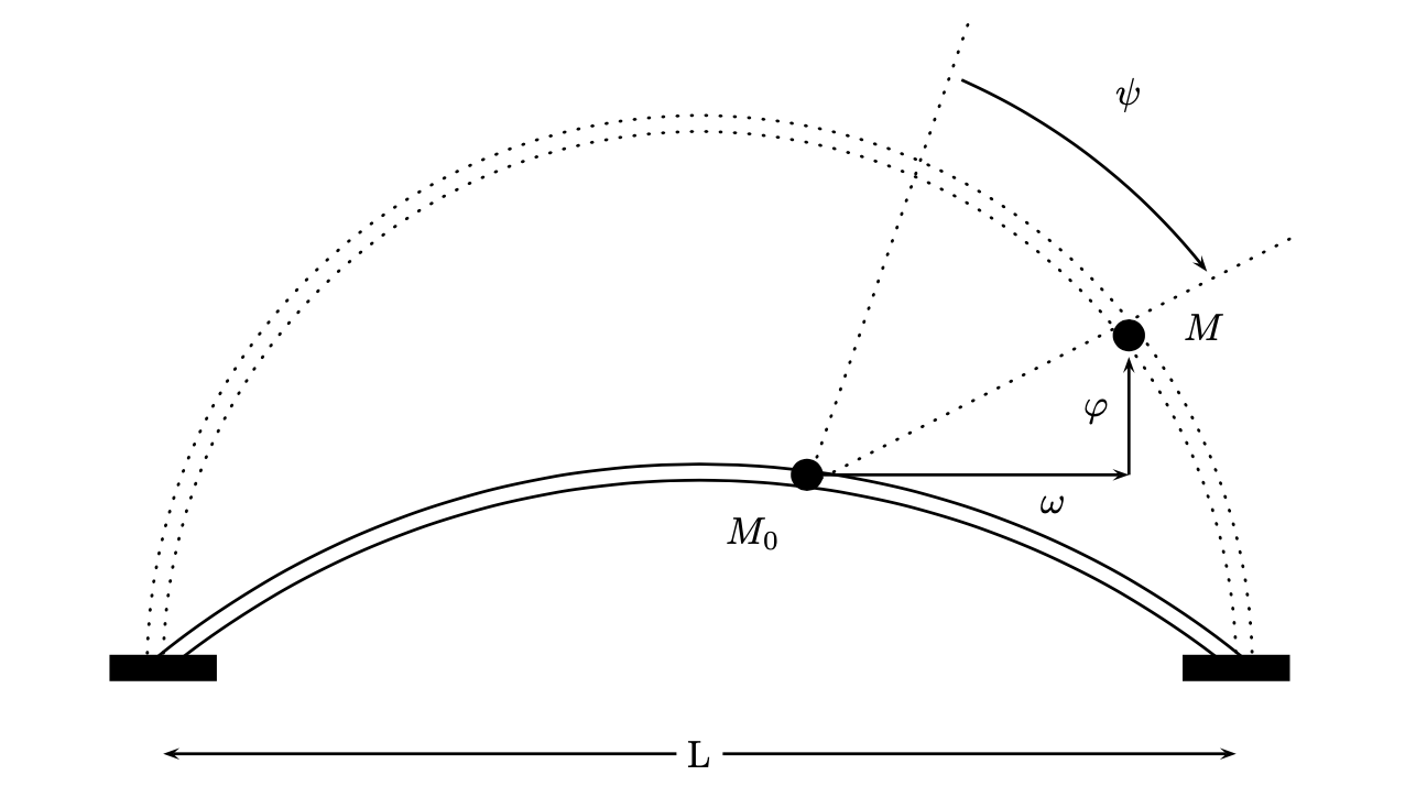
Figure 1. After deformation the particle $M_{0}$ of the beam is at the position $M$.

So we will consider the system of partial differential equations given on $\left(0,L\right)\times\left(0,+\infty\right)$ by the following form:

(1.1) $$\left\{\begin{array}[]{lll}\displaystyle{\rho_{1}\varphi_{tt}-[k_{1}\left(\varphi_{x}+\psi+\ell w\right)+D_{1}\left(\varphi_{xt}+\psi_{t}+\ell w_{t}\right)]_{x}-\ell k_{3}\left(w_{x}-\ell\varphi\right)-\ell D_{3}\left(w_{xt}-\ell\varphi_{t}\right)=0,}\\ \\ \displaystyle{\rho_{2}\psi_{tt}-[k_{2}\psi_{x}+D_{2}\psi_{xt}]_{x}+k_{1}\left(\varphi_{x}+\psi+\ell w\right)+D_{1}\left(\varphi_{xt}+\psi_{t}+\ell w_{t}\right)=0,}\\ \\ \displaystyle{\rho_{1}w_{tt}-[k_{3}\left(w_{x}-\ell\varphi\right)+D_{3}\left(w_{xt}-\ell\varphi_{t}\right)]_{x}+\ell k_{1}\left(\varphi_{x}+\psi+\ell w\right)+\ell D_{1}\left(\varphi_{xt}+\psi_{t}+\ell w_{t}\right)=0,}\end{array}\right.$$

with fully Dirichlet boundary conditions:

(1.2) $$\begin{array}[]{lll}\varphi\left(0,\cdot\right)=\varphi\left(L,\cdot\right)=\psi\left(0,\cdot\right)=\psi\left(L,\cdot\right)=w\left(0,\cdot\right)=w\left(L,\cdot\right)=0&\text{in }\mathbb{R}_{+},\end{array}$$

or with Dirichlet-Neumann-Neumann boundary conditions:

(1.3) $$\begin{array}[]{lll}\varphi\left(0,\cdot\right)=\varphi\left(L,\cdot\right)=\psi_{x}\left(0,\cdot\right)=\psi_{x}\left(L,\cdot\right)=w_{x}\left(0,\cdot\right)=w_{x}\left(L,\cdot\right)=0&\text{in }\mathbb{R}_{+},\end{array}$$

in addition to the following initial conditions:

(1.4) $$\begin{array}[]{lll}\varphi\left(\cdot,0\right)=\varphi_{0}\left(\cdot\right),\ {\psi\left(\cdot,0\right)=\psi_{0}\left(\cdot\right)},\ \par w\left(\cdot,0\right)=w_{0}\left(\cdot\right),\\ \vskip 6.0pt plus 2.0pt minus 2.0pt\cr\varphi_{t}\left(\cdot,0\right)=\varphi_{1}\left(\cdot\right),\ \psi_{t}\left(\cdot,0\right)=\psi_{1}\left(\cdot\right),\ w_{t}\left(\cdot,0\right)=w_{1}\left(\cdot\right),\ \ \ \text{in}\ (0,L).\\ \end{array}$$

We define the three wave speeds as:

$$c_{1}=\sqrt{\dfrac{k_{1}}{\rho_{1}}}\quad,\quad c_{2}=\sqrt{\dfrac{k_{2}}{\rho_{2}}}\quad,\quad c_{3}=\sqrt{\dfrac{k_{3}}{\rho_{1}}}\quad.$$

In the absence of the three Kelvin-Voigt damping terms, the system (1.1) is a system of three coupled wave equations. This system is conservative whereas when at least one of the three Kelvin-Voigt damping is present, the system is dissipative. The combination of direct damping, that is damping that acts in the equation involving the unknown itself and indirect damping that acts on another unknown than the one concerns by the equation, makes this study much delicate.

We note that when $R\rightarrow\infty$, then $\ell\rightarrow 0$ and the Bresse model reduces, by neglecting $w$, to the well-known Timoshenko beam equations:

(1.5) $$\left\{\begin{array}[]{lll}\displaystyle{\rho_{1}\varphi_{tt}-[k_{1}\left(\varphi_{x}+\psi\right)+D_{1}\left(\varphi_{xt}+\psi_{t}\right)]_{x}=0,}\\ \\ \displaystyle{\rho_{2}\psi_{tt}-[k_{2}\psi_{x}+D_{2}\psi_{xt}]_{x}+k_{1}\left(\varphi_{x}+\psi\right)+D_{1}\left(\varphi_{xt}+\psi_{t}\right)=0}\end{array}\right.$$

with different types of boundary conditions and with initial data.

1.2. Motivation, aims and main results

The stability of elastic Bresse system with different types of damping (frictional, thermoelastic, Cattaneo, …) has been intensively studied (see Subsection 1.3), but there are a few number of papers concerning the stability of Bresse or Timoshenko systems with local viscoelastic Kelvin-Voigt damping. In fact, in [7], El Arwadi and Youssef studied the theoretical and numerical stability on a Bresse system with Kelvin-Voigt damping under fully Dirichlet boundary conditions. Using multiplier techniques, they established an exponential energy decay rate provided that the system is subject to three global Kelvin-Voigt damping. Later, a numerical scheme based on the finite element method was introduced to approximate the solution. Zhao et al. in [25], considered a Timoshenko system with Dirichlet-Neumann boundary conditions. They obtained the exponential stability under certain hypotheses of the smoothness and structural condition of the coefficients of the system, and obtain the strong asymptotic stability under weaker hypotheses of the coefficients. Tian and Zhang in [23] considered a Timoshenko system under fully Dirichlet boundary conditions and with two locally or globally Kelvin-Voigt dampings. First, in the case when the two Kelvin-Voigt dampings are globally distributed, they showed that the corresponding semigroup is analytic. On the contrary, they proved that the energy of the system decays exponentially or polynomially and the decay rate depends on properties of material coefficient function. In [9], Ghader and Wehbe generalized the results of [25] and [23]. Indeed, they considered the Timoshenko system with only one locally or globally distributed Kelvin-Voigt damping and subject to fully Dirichlet or to Dirichlet-Neumann boundary conditions. They established a polynomial energy decay rate of type $t^{-1}$ for smooth initial data. Moreover, they proved that the obtained energy decay rate is in some sense optimal. In [19], Maryati et al. considered the transmission problem of a Timoshenko beam composed by $N$ components, each of them being either purely elastic, or a Kelvin-Voigt viscoelastic material, or an elastic material inserted with a frictional damping mechanism. They proved that the energy decay rate depends on the position of each component. In particular, they proved that the model is exponentially stable if and only if all the elastic components are connected with one component with frictional damping. Otherwise, only a polynomial energy decay rate is established. So, the stability of the Bresse system with local viscoelastic Kelvin-Voigt damping is still an open problem.

The purpose of this paper is to study the Bresse system in the presence of local non-smooth dampings coefficient at interface and under fully Dirichlet or Dirichlet-Neumann-Neumann boundary conditions. The system is given by (1.1)-(1.2) or (1.1)-(1.3) with initial data (1.4).

When $D_{1}$, $D_{2}$, $D_{3}\in L^{\infty}(0,L)$, using frequency domain approach combined with multiplier techniques and the construction of new multiplier functions, we establish a polynomial stability of type $\dfrac{1}{t}$ (see Theorem 4.2). Moreover, in the presence of only one local damping $D_{2}$ acting on the shear angle displacement ($D_{1}=D_{3}=0$), we establish a polynomial energy decay estimate of type $\dfrac{1}{\sqrt{t}}$ (see Theorem 5.1).

Finally, in the absence of at least one damping, we prove the lack of uniform stability for the system (1.1)-(1.3) even with smoothness of damping coefficients. In these cases, we conjecture the optimality of the obtained decay rate. For clarity, let

$$\emptyset\not=\omega=(\alpha,\beta)\subset(0,L).$$

Here and thereafter, $\alpha$ and $\beta$ will be considered as interfaces.

1.3. Literature concerning the Bresse system

In [17], Liu and Rao considered the Bresse system with two thermal dissipation laws. They proved an exponential decay rate when the wave speed of the vertical displacement coincides with the wave speed of longitudinal displacement or of the shear angle displacement. Otherwise, they showed polynomial decays depending on the boundary conditions. These results are improved by Fatori and Rivera in [8] where they considered the case of one thermal dissipation law globally distributed on the displacement equation. Wehbe and Najdi in [20] extended and improved the results of [8], when the thermal dissipation is locally distributed. Wehbe and Youssef in [24] considered an elastic Bresse system subject to two locally internal dissipation laws. They proved that the system is exponentially stable if and only if the waves propagate at the same speed. Otherwise, a polynomial decay holds. Alabau et al. in [2] considered the same system with one globally distributed dissipation law. The authors proved the existence of polynomial decays with rates that depend on some particular relation between the coefficients. In [10], Guesmia et al. considered Bresse system with infinite memories acting in the three equations of the system. They established asymptotic stability results under some conditions on the relaxation functions regardless the speeds of propagation. These results are improved by Abdallah et al. in [1] where they considered the Bresse system with infinite memory type control and/or with heat conduction given by Cattaneo’s law acting in the shear angle displacement. The authors established an exponential energy decay rate when the waves propagate at same speed. Otherwise, they showed polynomial decays. In [4], Benaissa and Kasmi, considered the Bresse system with three control of fractional derivative type acting on the boundary conditions. They established a polynomial decay estimate.

1.4. Organization of the paper

This paper is organized as follows: In Section 2, we prove the well-posedness of system (1.1) with either the boundary conditions (1.2) or (1.3). Next, in Section 3, we prove the strong stability of the system in the lack of the compactness of the resolvent of the generator.

In Section 4 when the coefficient functions $D_{1}$, $D_{2}$, and $D_{3}$ are not smooth, we prove the polynomial stability of type $\frac{1}{t}$. In section 5, we prove the polynomial energy decay rate of type $\frac{1}{\sqrt{t}}$ for the system in the case of only one local non-smooth damping $D_{2}$ acting on the shear angle displacement. In Section 6, under boundary conditions (1.3), we prove the lack of uniform (exponential) stability of the system in the absence of at least one damping. Finally in Section 7, we will briefly state the analytic stabilization of the system (1.1) when the three damping coefficient act on the whole spatial domain $(0,L)$ and the exponential stability when the three damping coefficient are localized on $(\alpha,\beta)$ and are smooth at the interfaces.

2. Well-posedness of the problem

In this part, using a semigroup approach, we establish the well-posedness result for the systems (1.1)-(1.2) and (1.1)-(1.3). Let $(\varphi,\psi,w)$ be a regular solution of system (1.1)-(1.2), its associated energy is given by:

(2.1) $$\begin{array}[]{ll}\displaystyle{E\left(t\right)}=\displaystyle{\frac{1}{2}\bigg{\{}\int_{0}^{L}\left(\rho_{1}\left|\varphi_{t}\right|^{2}+\rho_{2}\left|\psi_{t}\right|^{2}+\rho_{1}\left|w_{t}\right|^{2}+k_{1}\left|\varphi_{x}+\psi+\ell w\right|^{2}\right)dx}\\ \vskip 6.0pt plus 2.0pt minus 2.0pt\cr\hskip 45.52458pt\displaystyle{+\int_{0}^{L}\left({k}_{2}\left|\psi_{x}\right|^{2}+k_{3}\left|w_{x}-\ell\varphi\right|^{2}\right)dx}\bigg{\}},\end{array}$$

and it is dissipated according to the following law:

(2.2) $$E^{\prime}\left(t\right)=-\int_{0}^{L}\left(D_{1}|\varphi_{xt}+\psi_{t}+\ell w_{t}|^{2}+D_{2}|\psi_{xt}|^{2}+D_{3}|w_{xt}-\ell\varphi_{t}|^{2}\right)dx\leq 0.$$

Now, we define the following energy spaces:

$$\mathcal{H}_{1}=\left(H_{0}^{1}(0,L)\times L^{2}(0,L)\right)^{3}\ \ \mathrm{and}\ \ \mathcal{H}_{2}=H_{0}^{1}(0,L)\times L^{2}(0,L)\times\left(H_{*}^{1}(0,L)\times L^{2}_{*}(0,L)\right)^{2},$$

where

$$L_{*}^{2}(0,L)=\{f\in L^{2}(0,L):\int_{0}^{L}f(x)dx=0\}\,\,{\rm and}\,\,H_{*}^{1}(0,L)=\{f\in H^{1}(0,L):\int_{0}^{L}f(x)dx=0\}.$$

Both spaces $\mathcal{H}_{1}$ and $\mathcal{H}_{2}$ are equipped with the inner product which induces the energy norm:

(2.3) $$\begin{array}[]{ll}\displaystyle{\|U\|_{\mathcal{H}_{j}}^{2}}&=\displaystyle{\|(v^{1},v^{2},v^{3},v^{4},v^{5},v^{6})\|_{\mathcal{H}_{j}}^{2}}\\ &=\rho_{1}\left\|v^{2}\right\|^{2}+\rho_{2}\left\|v^{4}\right\|^{2}+\rho_{1}\left\|v^{6}\right\|^{2}+k_{1}\left\|v^{1}_{x}+v^{3}+\ell v^{5}\right\|^{2}\\ \vskip 6.0pt plus 2.0pt minus 2.0pt\cr&+{k}_{2}\left\|v^{3}_{x}\right\|^{2}+k_{3}\left\|v^{5}_{x}-\ell v^{1}\right\|^{2},\ \ j=1,2\end{array}$$

here and after $\|\cdot\|$ denotes the norm of $L^{2}\left(0,L\right)$ .

Remark 2.1.

In the case of boundary condition (1.2), it is easy to see that expression (2.3) defines a norm on the energy space $\mathcal{H}_{1}$. But in the case of boundary condition (1.3) the expression (2.3) define a norm on the energy space $\mathcal{H}_{2}$ if $L\neq\dfrac{n\pi}{\ell}$ for all positive integer $n$. Then, here and after, we assume that there does not exist any $n\in\mathbb{N}$ such that $L=\dfrac{n\pi}{\ell}$ when $j=2$.

Next, we define the linear operator $\mathcal{A}_{j}$ in $\mathcal{H}_{j}$ by:

$$\begin{array}[]{l}D\left(\mathcal{A}_{1}\right)=\bigg{\{}\ U\in\mathcal{H}_{1}\ |\ v^{2},v^{4},v^{6}\in H_{0}^{1}\left(0,L\right),\ \left[k_{1}\left(v_{x}^{1}+v^{3}+\ell v^{5}\right)+D_{1}\left(v_{x}^{2}+v^{4}+\ell v^{6}\right)\right]_{x}\in L^{2}(0,L)\,,\\ \hskip 85.35826pt\ \left[k_{2}v_{x}^{3}+D_{2}v_{x}^{4}\right]_{x}\in L^{2}(0,L),\,\left[k_{3}(v_{x}^{5}-\ell v^{1})+D_{3}(v_{x}^{6}-\ell v^{2})\right]_{x}\in L^{2}(0,L)\bigg{\}},\end{array}$$

$$\begin{array}[]{l}D\left(\mathcal{A}_{2}\right)=\bigg{\{}\ U\in\mathcal{H}_{2}\ |\ v^{2}\in H_{0}^{1}\left(0,L\right),v^{4},v^{6}\in H_{*}^{1}\left(0,L\right),v^{3}_{x}|_{0,L}=v^{5}_{x}|_{0,L}=0,\\ \hskip 85.35826pt\ \left[k_{1}\left(v_{x}^{1}+v^{3}+\ell v^{5}\right)+D_{1}\left(v_{x}^{2}+v^{4}+\ell v^{6}\right)\right]_{x}\in L^{2}(0,L)\,,\\ \hskip 85.35826pt\ \left[k_{2}v_{x}^{3}+D_{2}v_{x}^{4}\right]_{x}\in L_{*}^{2}(0,L),\,\left[k_{3}(v_{x}^{5}-\ell v^{1})+D_{3}(v_{x}^{6}-\ell v^{2})\right]_{x}\in L_{*}^{2}(0,L)\bigg{\}}\end{array}$$

and

(2.4) $$\mathcal{A}_{j}\left(\begin{array}[]{l}v^{1}\\ \vskip 6.0pt plus 2.0pt minus 2.0pt\cr v^{2}\\ \vskip 6.0pt plus 2.0pt minus 2.0pt\cr v^{3}\\ v^{4}\\ \vskip 6.0pt plus 2.0pt minus 2.0pt\cr v^{5}\\ \vskip 6.0pt plus 2.0pt minus 2.0pt\cr v^{6}\end{array}\right)=\left(\begin{array}[]{c}v^{2}\\ \vskip 6.0pt plus 2.0pt minus 2.0pt\cr\rho_{1}^{-1}\left(\left[k_{1}(v_{x}^{1}+v^{3}+\ell v^{5})+D_{1}(v_{x}^{2}+v^{4}+\ell v^{6})\right]_{x}+\ell k_{3}(v_{x}^{5}-\ell v^{1})+\ell D_{3}(v_{x}^{6}-\ell v^{2})\right)\\ \vskip 6.0pt plus 2.0pt minus 2.0pt\cr v^{4}\\ \vskip 6.0pt plus 2.0pt minus 2.0pt\cr\rho_{2}^{-1}\left((k_{2}v_{x}^{3}+D_{2}v_{x}^{4})_{x}-k_{1}\left(v^{1}_{x}+v^{3}+\ell v^{5}\right)-D_{1}(v_{x}^{2}+v^{4}+\ell v^{6})\right)\\ \vskip 6.0pt plus 2.0pt minus 2.0pt\cr v^{6}\\ \vskip 6.0pt plus 2.0pt minus 2.0pt\cr\rho_{1}^{-1}\left(\left[k_{3}(v^{5}_{x}-\ell v^{1})+D_{3}(v_{x}^{6}-\ell v^{2})\right]_{x}-\ell k_{1}\left(v^{1}_{x}+v^{3}+\ell v^{5}\right)-\ell D_{1}(v_{x}^{2}+v^{4}+\ell v^{6})\right)\end{array}\right)$$

for all $U=\left(v^{1},v^{2},v^{3},v^{4},v^{5},v^{6}\right)^{\mathsf{T}}\in D\left(\mathcal{A}_{j}\right)$. So, if $U=\left(\varphi,\varphi_{t},\psi,\psi_{t},w,w_{t}\right)^{\mathsf{T}}$ is the state of (1.1)-(1.2) or (1.1)-(1.3), then the Bresse beam system is transformed into a first order evolution equation on the Hilbert space $\mathcal{H}_{j}$:

(2.5) $$\left\{\begin{array}[]{c}U_{t}=\mathcal{A}_{j}U,\,\,j=1,2\\ \vskip 6.0pt plus 2.0pt minus 2.0pt\cr U\left(0\right)=U_{0}(x),\end{array}\right.$$

where

$$U_{0}\left(x\right)=\left(\varphi_{0}\left(x\right),\varphi_{1}\left(x\right),{\psi_{0}\left(x\right)},\psi_{1}\left(x\right),w_{0}\left(x\right),w_{1}\left(x\right)\right)^{\mathsf{T}}.$$

Remark 2.2.

It is easy to see that there exists a positive constant $c_{0}$ such that for any $\left(\varphi,\psi,w\right)\in\left(H_{0}^{1}\left(0,L\right)\right)^{3}$ for $j=1$ and for any $\left(\varphi,\psi,w\right)\in H_{0}^{1}\left(0,L\right)\times\left(H_{*}^{1}\left(0,L\right)\right)^{2}$ for $j=2$,

(2.6) $$k_{1}\left\|\varphi_{x}+\psi+\ell w\right\|^{2}+{k}_{2}\left\|\psi_{x}\right\|^{2}+k_{3}\left\|w_{x}-\ell\varphi\right\|^{2}\leq c_{0}\left(\left\|\varphi_{x}\right\|^{2}+\left\|\psi_{x}\right\|^{2}+\left\|w_{x}\right\|^{2}\right).$$

On the other hand, we can show by a contradiction argument the existence of a positive constant $c_{1}$ such that, for any $\left(\varphi,\psi,w\right)\in\left(H_{0}^{1}\left(0,L\right)\right)^{3}$ for $j=1$ and for any $\left(\varphi,\psi,w\right)\in H_{0}^{1}\left(0,L\right)\times\left(H_{*}^{1}\left(0,L\right)\right)^{2}$ for $j=2$,

(2.7) $$c_{1}\left(\left\|\varphi_{x}\right\|^{2}+\left\|\psi_{x}\right\|^{2}+\left\|w_{x}\right\|^{2}\right)\leq k_{1}\left\|\varphi_{x}+\psi+\ell w\right\|^{2}+{k}_{2}\left\|\psi_{x}\right\|^{2}+k_{3}\left\|w_{x}-\ell\varphi\right\|^{2}.$$

Therefore the norm on the energy space $\mathcal{H}_{j}$ given in (2.3) is equivalent to the usual norm on $\mathcal{H}_{j}$.

Proposition 2.3.

Assume that coefficients functions $D_{1}$, $D_{2}$ and $D_{3}$ are non negative. Then, the operator $\mathcal{A}_{j}$ is m-dissipative in the energy space $\mathcal{H}_{j}$, for $j=1,2$.

Proof.

Let $U=\left(v^{1},v^{2},v^{3},v^{4},v^{5},v^{6}\right)^{\mathsf{T}}\in D\left(\mathcal{A}_{j}\right)$. By a straightforward calculation, we have:

(2.8) $$\mathrm{Re}\left(\mathcal{A}_{j}U,U\right)_{\mathcal{H}_{j}}=-\int_{0}^{L}\left(D_{1}\left|v_{x}^{2}+v^{4}+\ell v^{6}\right|^{2}+D_{2}\left|v_{x}^{4}\right|^{2}+D_{3}\left|v_{x}^{6}-\ell v^{2}\right|^{2}\right)dx.$$

As $D_{1}\geq 0,\,D_{2}\geq 0\,\,\mathrm{and}\,D_{3}\geq 0$ , we get that $\mathcal{A}_{j}$ is dissipative.

Now, we will check the maximality of $\mathcal{A}_{j}$. For this purpose, let $F=\left(f^{1},f^{2},f^{3},f^{4},f^{5},f^{6}\right)^{\mathsf{T}}\in\mathcal{H}_{j},$ we have to prove the existence of $U=\left(v^{1},v^{2},v^{3},v^{4},v^{5},v^{6}\right)^{\mathsf{T}}\in D\left(\mathcal{A}_{j}\right)$ unique solution of the equation $-\mathcal{A}_{j}U=F$.

Let $\left(\varphi^{1},\varphi^{3},\varphi^{5}\right)\in\left(H_{0}^{1}(0,L)\right)^{3}$ for $j=1$ and $\left(\varphi^{1},\varphi^{3},\varphi^{5}\right)\in\left(H_{0}^{1}(0,L)\times(H_{*}^{1}(0,L))^{2}\right)$ for $j=2$ be a test function. Writing $-\mathcal{A}_{j}U$ and replacing the first, third and fith component of $U$ by $-f^{1}\,,\,-f^{3}\,,\,-f^{5}$ and now multiplying the second, the fourth and the sixth equation by respectively $\varphi^{1},\varphi^{3},\varphi^{5}$, after integrating by parts, we obtain the following form:

(2.9) $$\left\{\begin{array}[]{ll}\displaystyle{k_{1}\left(v^{1}_{x}+v^{3}+\ell v^{5}\right)\varphi^{1}_{x}-\ell k_{3}\left(v^{5}_{x}-\ell v^{1}\right)\varphi^{1}=h^{1},}\\ \vskip 6.0pt plus 2.0pt minus 2.0pt\cr\displaystyle{k_{2}v^{3}_{x}\varphi_{x}^{3}+k_{1}\left(v^{1}_{x}+v^{3}+\ell v^{5}\right)\varphi^{3}=h^{3}},\\ \vskip 6.0pt plus 2.0pt minus 2.0pt\cr\displaystyle{k_{3}\left(v^{5}_{x}-\ell v^{1}\right)\varphi_{x}^{5}+\ell k_{1}\left(v^{1}_{x}+v^{3}+\ell v^{5}\right)\varphi^{5}=h^{5},}\end{array}\right.$$

where

$$h^{1} =\rho_{1}f^{2}\varphi^{1}+D_{1}\left(f_{x}^{1}+f^{3}+\ell f^{5}\right)\varphi_{x}^{1}-\ell D_{3}(f_{x}^{5}-\ell f^{1})\varphi^{1},$$

$$h^{3} =\rho_{2}f^{4}\varphi^{3}+D_{2}f_{x}^{3}\varphi_{x}^{3}+D_{1}\left(f_{x}^{1}+f^{3}+\ell f^{5}\right)\varphi^{3},\mbox{ and}$$

$$h^{5} =\rho_{1}f^{6}\varphi^{5}+D_{3}\left(f^{5}-\ell f^{1}\right)\varphi_{x}^{5}+\ell D_{1}\left(f_{x}^{1}+f^{3}+\ell f^{5}\right)\varphi^{5}.$$

Using Lax-Milgram Theorem (see [21]), we deduce that (2.9) admits a unique solution in $\left(H^{1}_{0}\left(0,L\right)\right)^{3}$ for $j=1$ and in $\left(H_{0}^{1}(0,L)\times(H_{*}^{1}(0,L))^{2}\right)$ for $j=2$. Thus, $-\mathcal{A}_{j}U=F$ admits an unique solution $U\in D\left(\mathcal{A}_{j}\right)$ and consequently $0\in\rho(\mathcal{A}_{j})$. Then, $\mathcal{A}_{j}$ is closed and consequently $\rho\left(\mathcal{A}_{j}\right)$ is open set of $\mathbb{C}$ (see Theorem 6.7 in [13]). Hence, we easily get $R(\lambda I-\mathcal{A}_{j})=\mathcal{H}_{j}$ for sufficiently small $\lambda>0$. This, together with the dissipativeness of $\mathcal{A}_{j}$, imply that $D\left(\mathcal{A}_{j}\right)$ is dense in $\mathcal{H}_{j}$ and that $\mathcal{A}_{j}$ is m-dissipative in $\mathcal{H}_{j}$ (see Theorems 4.5, 4.6 in [21]). The proof is thus complete.

∎

Thanks to Lumer-Phillips Theorem (see [18, 21]), we deduce that $\mathcal{A}_{j}$ generates a $C_{0}$-semigroup of contraction $e^{t\mathcal{A}_{j}}$ in $\mathcal{H}_{j}$ and therefore problem (2.5) is well-posed. We have thus the following result.

Theorem 2.4.

For any $U_{0}\in\mathcal{H}_{j}$, problem (2.5) admits a unique weak solution

$$U\in C\left(\mathbb{R}_{+};\mathcal{H}_{j}\right).$$

Moreover, if $U_{0}\in D\left(\mathcal{A}_{j}\right),$ then

$$U\in C\left(\mathbb{R}_{+};D\left(\mathcal{A}_{j}\right)\right)\cap C^{1}\left(\mathbb{R}_{+};\mathcal{H}_{j}\right).$$

3. Strong stability of the system

In this part, we use a general criteria of Arendt-Batty in [3] to show the strong stability of the $C_{0}$-semigroup $e^{t\mathcal{A}_{j}}$ associated to the Bresse system (1.1) in the absence of the compactness of the resolvent of $\mathcal{A}_{j}$. Before, we state our main result, we need the following stability condition:

$$\mbox{(SSC)}\quad\quad\mbox{There exist}\,i\in\{1,2,3\},\,d_{0}>0\,\,\mathrm{and}\,\,\alpha<\beta\in[0,L]\,\mbox{such that}\,\,D_{i}\geq d_{0}>0\,\,\mathrm{on}\,\,(\alpha,\beta).$$

Theorem 3.1.

Assume that condition (SSC) holds. Then the $C_{0}-$semigroup $e^{t\mathcal{A}_{j}}$ is strongly stable in $\mathcal{H}_{j}$, $j=1,2$, i.e., for all $U_{0}\in\mathcal{H}_{j}$, the solution of (2.5) satisfies

$$\lim_{t\to+\infty}\left\|e^{t\mathcal{A}_{j}}U_{0}\right\|_{\mathcal{H}_{j}}=0.$$

For the proof of Theorem 3.1, we need the following two lemmas.

Lemma 3.2.

Under the same condition of Theorem 3.1, we have

(3.1) $$\ker\left(\ i\lambda-\mathcal{A}_{j}\right)=\{0\},\,\,j=1,2,\,\,\,{\rm for\,all}\,\,\lambda\in\mathbb{R}.$$

Proof.

We will prove Lemma 3.2 in the case $D_{1}=D_{3}=0$ on $(0,L)$ and $D_{2}\geq d_{0}>0$ on $(\alpha,\beta)\subset(0,L)$. The other cases are similar to prove.
First, from Proposition 2.3, we claim that $0\in\rho\left(\mathcal{A}_{j}\right).$ We still have to show the result for $\lambda\in\mathbb{R^{*}}$. Suppose that there exist a real number $\lambda\neq 0$ and $0\neq U=\left(v^{1},v^{2},v^{3},v^{4},v^{5},v^{6}\right)^{\mathsf{T}}\in D\left(\mathcal{A}_{j}\right)$ such that:

(3.2) $$\mathcal{A}_{j}U=\ i\lambda U.$$

Our goal is to find a contradiction by proving that $U=0$. Taking the real part of the inner product in $\mathcal{H}_{j}$ of $\mathcal{A}_{j}U$ and $U$, we get:

(3.3) $$\mathrm{Re}\left(\mathcal{A}_{j}U,U\right)_{\mathcal{H}_{j}}=-\int_{0}^{L}D_{2}\left|v_{x}^{4}\right|^{2}dx=0.$$

Since by assumption $D_{2}\geq d_{0}>0$ on $(\alpha,\beta)$, it follows from equality (3.3) that:

(3.4) $$D_{2}v^{4}_{x}=0\quad\mathrm{in}\quad(0,L)\,\,\mathrm{and}\,\,v^{4}_{x}=0\quad\mathrm{in}\quad(\alpha,\beta).$$

Detailing (3.2) we get:

(3.5) $$v^{2} = \ i\lambda v^{1},$$

(3.6) $$k_{1}\left(v^{1}_{x}+v^{3}+\ell v^{5}\right)_{x}+\ell k_{3}\left(v^{5}_{x}-\ell v^{1}\right) = \ i\rho_{1}\lambda v^{2},$$

(3.7) $$v^{4} = \ i\lambda v^{3},$$

(3.8) $$\left(k_{2}v^{3}_{x}+D_{2}v^{4}_{x}\right)_{x}-k_{1}\left(v^{1}_{x}+v^{3}+\ell v^{5}\right) = \ i\rho_{2}\lambda v^{4},$$

(3.9) $$v^{6} = \ i\lambda v^{5},$$

(3.10) $$k_{3}\left(v^{5}_{x}-\ell v^{1}\right)_{x}-\ell k_{1}\left(v^{1}_{x}+v^{3}+\ell v^{5}\right) = \ i\rho_{1}\lambda v^{6}.$$

Next, inserting (3.4) in (3.7) and using the fact that $\lambda\neq 0$, we get:

(3.11) $$v^{3}_{x}=0\quad\mathrm{in}\quad(\alpha,\beta).$$

Moreover, substituting equations (3.5), (3.7) and (3.9) into equations (3.6), (3.8) and (3.10), we get:

(3.12) $$\left\{\begin{array}[]{ll}\rho_{1}\lambda^{2}v^{1}+k_{1}\left(v^{1}_{x}+v^{3}+\ell v^{5}\right)_{x}+\ell k_{3}\left(v^{5}_{x}-\ell v^{1}\right)=0,\\ \vskip 6.0pt plus 2.0pt minus 2.0pt\cr\rho_{2}\lambda^{2}v^{3}+\left(k_{2}v^{3}_{x}+iD_{2}\lambda v^{3}_{x}\right)_{x}-k_{1}\left(v^{1}_{x}+v^{3}+\ell v^{5}\right)=0,\\ \vskip 6.0pt plus 2.0pt minus 2.0pt\cr\rho_{1}\lambda^{2}v^{5}+k_{3}\left(v^{5}_{x}-\ell v^{1}\right)_{x}-\ell k_{1}\left(v^{1}_{x}+v^{3}+\ell v^{5}\right)=0.\end{array}\right.$$

Now, we introduce the functions $\widehat{v}^{i}$, for $i=1,..,6$ by $\widehat{v}^{i}=v_{x}^{i}\ .$ It is easy to see that $\widehat{v}^{i}\in H^{1}(0,L)$.
It follows from equations (3.4) and (3.11) that:

(3.13) $$\widehat{v}^{3}=\widehat{v}^{4}=0\quad\mathrm{in}\quad(\alpha,\beta)$$

and consequently system (3.12) will be, after differentiating it with respect to $x$, given by:

(3.14) $$\rho_{1}\lambda^{2}\widehat{v}^{1}+k_{1}\left(\widehat{v}^{1}_{x}+\ell\widehat{v}^{5}\right)_{x}+\ell k_{3}\left(\widehat{v}^{5}_{x}-\ell\widehat{v}^{1}\right) = 0\quad\mathrm{in}\quad(\alpha,\beta),$$

(3.15) $$\widehat{v}^{1}_{x}+\ell\widehat{v}^{5} = 0\quad\mathrm{in}\quad(\alpha,\beta),$$

(3.16) $$\rho_{1}\lambda^{2}\widehat{v}^{5}+k_{3}\left(\widehat{v}^{5}_{x}-\ell\widehat{v}^{1}\right)_{x}-\ell k_{1}\left(\widehat{v}^{1}_{x}+\ell\widehat{v}^{5}\right) = 0\quad\mathrm{in}\quad(\alpha,\beta).$$

Furthermore, substituting equation (3.15) into (3.14) and (3.16), we get:

(3.17) $$\rho_{1}\lambda^{2}\widehat{v}^{1}+\ell k_{3}\left(\widehat{v}^{5}_{x}-\ell\widehat{v}^{1}\right) = 0\quad\mathrm{in}\quad(\alpha,\beta),$$

(3.18) $$\widehat{v}^{1}_{x}+\ell\widehat{v}^{5} = 0\quad\mathrm{in}\quad(\alpha,\beta),$$

(3.19) $$\rho_{1}\lambda^{2}\widehat{v}^{5}+k_{3}\left(\widehat{v}^{5}_{x}-\ell\widehat{v}^{1}\right)_{x} = 0\quad\mathrm{in}\quad(\alpha,\beta).$$

Differentiating equation (3.17) with respect to $x$, a straightforward computation with equation (3.19) yields:

$$\rho_{1}\lambda^{2}\left(\widehat{v}_{x}^{1}-\ell\widehat{v}^{5}\right)=0\quad\mathrm{in}\quad(\alpha,\beta).$$

Equivalently

(3.20) $$\widehat{v}_{x}^{1}-\ell\widehat{v}^{5}=0\quad\mathrm{in}\quad(\alpha,\beta).$$

Hence, from equations (3.18) and (3.20), we get:

(3.21) $$\widehat{v}^{5}=0\quad\mathrm{and}\quad\widehat{v}^{1}_{x}=0\quad\mathrm{in}\quad(\alpha,\beta).$$

Plugging $\widehat{v}^{5}=0$ in (3.17), we get:

(3.22) $$\left(\rho_{1}\lambda^{2}-\ell^{2}k_{3}\right)\widehat{v}^{1}=0.$$

In order to finish our proof, we have to distinguish two cases:
Case 1: $\lambda\neq\ell\ \sqrt{\dfrac{k_{3}}{\rho_{1}}}$.
Using equation (3.22) , we deduce that:

$$\widehat{v}^{1}=0\quad\mathrm{in}\quad(\alpha,\beta).$$

Setting $V=\left(\widehat{v}^{1},\widehat{v}^{1}_{x},\widehat{v}^{3},\widehat{v}^{3}_{x},\widehat{v}^{5},\widehat{v}^{5}_{x}\right)^{\mathsf{T}}$. By continuity of $\widehat{v}^{i}$ on $(0,L)$, we deduce that $V(\alpha)=0$. Then system (3.12) could be given as:

(3.23) $$\left\{\begin{matrix}V_{x}&=&BV,\ \ \ {\rm{in}}\ \ (0,\alpha)\\ V(\alpha)&=&0,\end{matrix}\right.$$

where

(3.24) $$B=\begin{pmatrix}0&1&0&0&0&0\\ \dfrac{-\lambda^{2}\rho_{1}+\ell^{2}k_{3}}{k_{1}}&0&0&-1&\dfrac{-\ell(k_{1}+k_{3})}{k_{1}}&0\\ 0&0&0&1&0&0\\ 0&\dfrac{k_{1}}{k_{2}+i\lambda D_{2}}&\dfrac{k_{1}-\lambda^{2}\rho_{2}}{k_{2}+i\lambda D_{2}}&0&\dfrac{\ell k_{1}}{k_{2}+i\lambda D_{2}}&0\\ 0&0&0&0&0&1\\ 0&\dfrac{\ell(k_{3}+k_{1})}{k_{3}}&\dfrac{\ell k_{1}}{k_{3}}&0&\dfrac{\ell^{2}k_{1}-\lambda^{2}\rho_{1}}{k_{3}}&0\end{pmatrix}.$$

Using ordinary differential equation theory, we deduce that system (3.23) has the unique trivial solution $V=0$ in $(0,\alpha)$. The same argument as above leads us to prove that $V=0$ on $(\beta,L)$. Consequently, we obtain $\widehat{v}^{1}=\widehat{v}^{3}=\widehat{v}^{5}=0$ on $(0,L)$. It follows that $\widehat{v}^{2}=\widehat{v}^{4}=\widehat{v}^{6}=0$ on $(0,L)$, thus $\widehat{U}=0$. This gives that $U=C$, where $C$ is a constant. Finally, from the boundary condition (1.2) or (1.3), we deduce that $U=0$.
Case 2: $\lambda=\ell\ \sqrt{\dfrac{k_{3}}{\rho_{1}}}$.
The fact that $\widehat{v}^{1}_{x}=0$ on $(\alpha,\beta)$, we get $\widehat{v}^{1}=c$ on $(\alpha,\beta)$, where $c$ is a constant. By continuity of $\widehat{v}^{1}$ on $(0,L)$, we deduce that $\widehat{v}^{1}(\alpha)=c$. We know also that $\widehat{v}^{3}=\widehat{v}^{5}=0$ on $(\alpha,\beta)$ from (3.13) and (3.21). Hence, setting $V(\alpha)=(c,0,0,0,0,0)^{\mathsf{T}}=V_{0}$, we can rewrite system (3.12) on $(0,\alpha)$ under the form:

$$\left\{\begin{matrix}V_{x}&=&\widehat{B}V,\\ V(\alpha)&=&V_{0},\end{matrix}\right.$$

where

$$\widehat{B}=\begin{pmatrix}0&1&0&0&0&0\\ 0&0&0&-1&\dfrac{-\ell(k_{1}+k_{3})}{k_{1}}&0\\ 0&0&0&1&0&0\\ 0&\dfrac{k_{1}}{k_{2}+i\ell\sqrt{\frac{k_{3}}{\rho_{1}}}D_{2}}&\dfrac{k_{1}-\lambda^{2}\rho_{2}}{k_{2}+i\ell\sqrt{\frac{k_{3}}{\rho_{1}}}\lambda D_{2}}&0&\dfrac{\ell k_{1}}{k_{2}+i\ell\sqrt{\frac{k_{3}}{\rho_{1}}}D_{2}}&0\\ 0&0&0&0&0&1\\ 0&\dfrac{\ell(k_{3}+k_{1})}{k_{3}}&\dfrac{\ell k_{1}}{k_{3}}&0&\dfrac{\ell^{2}(k_{1}-k_{3})}{k_{3}}&0\end{pmatrix}.$$

Introducing $\widetilde{V}=\left(\widehat{v}^{1}_{x},\widehat{v}^{3},\widehat{v}^{3}_{x},\widehat{v}^{5},\widehat{v}^{5}_{x}\right)^{\mathsf{T}}$ and

$$\widetilde{B}=\begin{pmatrix}0&0&-1&\dfrac{-\ell(k_{1}+k_{3})}{k_{1}}&0\\ 0&0&1&0&0\\ \dfrac{k_{1}}{k_{2}+i\ell\sqrt{\frac{k_{3}}{\rho_{1}}}D_{2}}&\dfrac{k_{1}-\lambda^{2}\rho_{2}}{k_{2}+i\ell\sqrt{\frac{k_{3}}{\rho_{1}}}\lambda D_{2}}&0&\dfrac{\ell k_{1}}{k_{2}+i\ell\sqrt{\frac{k_{3}}{\rho_{1}}}D_{2}}&0\\ 0&0&0&0&1\\ \dfrac{\ell(k_{3}+k_{1})}{k_{3}}&\dfrac{\ell k_{1}}{k_{3}}&0&\dfrac{\ell^{2}(k_{1}-k_{3})}{k_{3}}&0\end{pmatrix}.$$

Then system (3.12) could be given as:

(3.25) $$\left\{\begin{matrix}\widetilde{V}_{x}&=&\widetilde{B}\widetilde{V},\ \ \mathrm{in}\ \ (0,\alpha),\\ \widetilde{V}(\alpha)&=&0.\end{matrix}\right.$$

Using ordinary differential equation theory, we deduce that system (3.25) has the unique trivial solution $\widetilde{V}=0$ in $(0,\alpha)$. This implies that on $(0,\alpha)$, we have $\widehat{v}^{3}=\widehat{v}^{5}=0$. Consequently, $v^{3}=c_{3}$ and $v^{5}=c_{5}$ where $c_{3}$ and $c_{5}$ are constants. But using the fact that $v^{3}(0)=v^{5}(0)=0$, we deduce that $v^{3}=v^{5}=0$ on $(0,\alpha)$.
Substituting $v^{3}$ and $v^{5}$ by their values in the second equation of system (3.12), we get that $v^{1}_{x}=0$. This yields $v^{1}=c_{1}$, where $c_{1}$ is a constant. But as $v^{1}(0)=0$, we get: $v^{1}=0$ on $(0,\alpha)$. Thus $U=0$ on $(0,\alpha)$. The same argument as above leads us to prove that $U=0$ on $(\beta,L)$ and therefore $U=0$ on $(0,L)$. Thus the proof is complete. ∎

Lemma 3.3.

Under the same condition of Theorem 3.1, $(\ i\lambda I-\mathcal{A}_{j}),j=1,2$ is surjective for all $\lambda\in\mathbb{R}$.

Proof.

We will prove Lemma 3.3 in the case $D_{1}=D_{3}=0$ on $(0,L)$ and $D_{2}\geq d_{0}>0$ on $(\alpha,\beta)\subset(0,L)$ and the other cases are similar to prove.
Since $0\in\rho\left(\mathcal{A}_{j}\right)$, we still need to show the result for $\lambda\in\mathbb{R^{*}}$. For any

$$F=\left(f^{1},f^{2},f^{3},f^{4},f^{5},f^{6}\right)^{\mathsf{T}}\in\mathcal{H}_{j},\ \lambda\in\mathbb{R}^{*},$$

we prove the existence of

$$U=\left(v^{1},v^{2},v^{3},v^{4},v^{5},v^{6}\right)^{\mathsf{T}}\in D\left(\mathcal{A}_{j}\right)$$

solution of the following equation:

(3.26) $$\left(\ i\lambda I-\mathcal{A}_{j}\right)U=F.$$

Equivalently, we have the following system:

(3.27) $$\ i\lambda v^{1}-v^{2} = f^{1},$$

(3.28) $$\ \rho_{1}\ i\lambda v^{2}-k_{1}\left(v^{1}_{x}+v^{3}+\ell v^{5}\right)_{x}-\ell k_{3}\left(v^{5}_{x}-\ell v^{1}\right) = \rho_{1}f^{2},$$

(3.29) $$\ i\lambda v^{3}-v^{4} = f^{3},$$

(3.30) $$\rho_{2}\ i\lambda v^{4}-(k_{2}v^{3}_{x}+D_{2}v^{4}_{x})_{x}+k_{1}\left(v^{1}_{x}+v^{3}+\ell v^{5}\right) = \rho_{2}f^{4},$$

(3.31) $$\ i\lambda v^{5}-v^{6} = f^{5},$$

(3.32) $$\rho_{1}\ i\lambda v^{6}-k_{3}\left(v^{5}_{x}-\ell v^{1}\right)_{x}+\ell k_{1}\left(v^{1}_{x}+v^{3}+\ell v^{5}\right) = \rho_{1}f^{6}.$$

From (3.27),(3.29) and (3.31), we have:

(3.33) $$v^{2}=\ i\lambda v^{1}-f^{1},\quad v^{3}=\ i\lambda v^{3}-f^{3},\quad v^{6}=\ i\lambda v^{5}-f^{5}.$$

Inserting (3.33) in (3.28), (3.30) and (3.32), we get:

(3.34) $$\left\{\begin{array}[]{ll}\displaystyle{-\lambda^{2}v^{1}-k_{1}\rho_{1}^{-1}\left(v^{1}_{x}+v^{3}+\ell v^{5}\right)_{x}-\ell k_{3}\rho_{1}^{-1}\left(v^{5}_{x}-\ell v^{1}\right)=h^{1},}\\ \vskip 6.0pt plus 2.0pt minus 2.0pt\cr\displaystyle{-\lambda^{2}v^{3}-\rho_{2}^{-1}\left(k_{2}+i\lambda D_{2}\right)v^{3}_{xx}+k_{1}\rho_{2}^{-1}\left(v^{1}_{x}+v^{3}+\ell v^{5}\right)=h^{3},}\\ \vskip 6.0pt plus 2.0pt minus 2.0pt\cr\displaystyle{-\lambda^{2}v^{5}-k_{3}\rho_{1}^{-1}\left(v^{5}_{x}-\ell v^{1}\right)_{x}+\ell k_{1}\rho_{1}^{-1}\left(v^{1}_{x}+v^{3}+\ell v^{5}\right)=h^{5},}\end{array}\right.$$

where

$${h^{1}=f^{2}+\ i\lambda f^{1},\quad h^{3}=f^{4}+\ i\lambda f^{3}-\rho_{2}^{-1}D_{2}f^{3}_{xx},\quad h^{5}=f^{6}+i\lambda f^{5}.}$$

For all $v=\left(v^{1},v^{3},v^{5}\right)^{\mathsf{T}}\in\left(H^{1}_{0}(0,L)\right)^{3}$ for $j=1$ and $v=\left(v^{1},v^{3},v^{5}\right)^{\mathsf{T}}\in H^{1}_{0}(0,L)\times H_{*}^{1}\left(0,L\right)^{2}$ for $j=2$, we define the linear operator $\mathcal{L}$ by:

$$\mathcal{L}v=\left(\begin{array}[]{c}\displaystyle{-k_{1}\rho_{1}^{-1}\left(v^{1}_{x}+v^{3}+\ell v^{5}\right)_{x}-\ell k_{3}\rho_{1}^{-1}\left(v^{5}_{x}-\ell v^{1}\right)}\\ \vskip 6.0pt plus 2.0pt minus 2.0pt\cr\displaystyle{-\rho_{2}^{-1}(k_{2}+i\lambda D_{2})v^{3}_{xx}+k_{1}\rho_{2}^{-1}\left(v^{1}_{x}+v^{3}+\ell v^{5}\right)}\\ \vskip 6.0pt plus 2.0pt minus 2.0pt\cr\displaystyle{-k_{3}\rho_{1}^{-1}\left(v^{5}_{x}-\ell v^{1}\right)_{x}+\ell k_{1}\rho_{1}^{-1}\left(v^{1}_{x}+v^{3}+\ell v^{5}\right)}\end{array}\right).$$

For clarity, we consider the case $j=1$. The proof in the case $j=2$ is very similar. Using Lax-Milgram theorem, it is easy to show that $\mathcal{L}$ is an isomorphism from $(H^{1}_{0}(0,L))^{3}$ onto $(H^{-1}\left(0,L\right))^{3}$. Let $v=\left(v^{1},v^{3},v^{5}\right)^{\mathsf{T}}$ and $h=\left(-h^{1},-h^{3},-h^{5}\right)^{\mathsf{T}}$, then we transform system (3.34) into the following form:

(3.35) $$(\lambda^{2}\mathcal{I}-\mathcal{L})v=h.$$

Since the operator $\mathcal{L}$ is an isomorphism from $(H^{1}_{0}(0,L))^{3}$ onto $(H^{-1}\left(0,L\right))^{3}$ and $\mathcal{I}$ is a compact operator from $(H^{1}_{0}(0,L))^{3}$ onto $(H^{-1}\left(0,L\right))^{3}$, then using Fredholm’s Alternative theorem, problem (3.35) admits a unique solution in $(H^{1}_{0}(0,L))^{3}$ if and only if $\lambda^{2}\mathcal{I}-\mathcal{L}$ is injective. For that purpose, let $\tilde{v}=\left(\tilde{v}^{1},\tilde{v}^{3},\tilde{v}^{5}\right)^{\mathsf{T}}$ in ${\rm ker}(\lambda^{2}\mathcal{I}-\mathcal{L})$. Then, if we set $\tilde{v}^{2}=i\lambda\tilde{v}^{1}$, $\tilde{v}^{4}=i\lambda\tilde{v}^{3}$ and $\tilde{v}^{6}=i\lambda\tilde{v}^{5}$, we deduce that $\tilde{V}=(\tilde{v}^{1},\tilde{v}^{2},\tilde{v}^{3},\tilde{v}^{5},\tilde{v}^{6})$ belongs to $D(\mathcal{A}_{1})$ and it is solution of:

$$(i\lambda\mathcal{I}-\mathcal{A}_{1})\tilde{V}=0.$$

Using Lemma 3.2, we deduce that $\tilde{v}^{1}=\tilde{v}^{3}=\tilde{v}^{5}=0$. This implies that equation (3.35) admits a unique solution in $v=(v^{1},v^{3},v^{5})\in(H^{1}_{0}(0,L))^{3}$ and

$${-k_{1}\rho_{1}^{-1}\left(v^{1}_{x}+v^{3}+\ell v^{5}\right)_{x}-\ell k_{3}\rho_{1}^{-1}\left(v^{5}_{x}-\ell v^{1}\right)}\in L^{2}(0,L),$$

$${-\rho_{2}^{-1}(k_{2}v^{3}_{x}+i\lambda D_{2}v^{3}_{x}-D_{2}f^{3}_{x})_{x}+k_{1}\rho_{2}^{-1}\left(v^{1}_{x}+v^{3}+\ell v^{5}\right)}\in L^{2}(0,L),$$

$${-k_{3}\rho_{1}^{-1}\left(v^{5}_{x}-\ell v^{1}\right)_{x}+\ell k_{1}\rho_{1}^{-1}\left(v^{1}_{x}+v^{3}+\ell v^{5}\right)}\in L^{2}(0,L).$$

By setting $v^{2}=\ i\lambda v^{1}-f^{1}$, $v^{3}=\ i\lambda v^{3}-f^{3}$ and $v^{6}=\ i\lambda v^{5}-f^{5}$, we deduce that $V=(v^{1},v^{2},v^{3},v^{4},v^{5},v^{6})$ belongs to $D(\mathcal{A}_{1})$ and it is the unique solution of equation (3.26) and the proof is thus complete. ∎

Proof of Theorem 3.1..

Following a general criteria of Arendt-Batty in [3], the $C_{0}-$semigroup $e^{t\mathcal{A}_{j}}$ of contractions is strongly stable if $\mathcal{A}_{j}$ has no pure imaginary eigenvalues and $\sigma(\mathcal{A}_{j})\cap i\mathbb{R}$ is countable. By Lemma 3.2, the operator $\mathcal{A}_{j}$ has no pure imaginary eigenvalues and by Lemma 3.3, ${\rm R}(\ i\lambda-\mathcal{A}_{j})=\mathcal{H}_{j}$ for all $\lambda\in\mathbb{R}$. Therefore the closed graph theorem of Banach implies that $\sigma(\mathcal{A}_{j})\cap i\mathbb{R}=\emptyset$. Thus, the proof is complete. ∎

4. Polynomial stability for non smooth damping coefficients at the interface

Before we state our main result, we recall the following results (see [11], [22] for part i), [5] for ii) and [21] for iii).

Theorem 4.1.

Let $\mathcal{A}:D(\mathcal{A})\subset\mathcal{H}\rightarrow\mathcal{H}$ be an unbounded operator generating a $C_{0}$-semigroup of contractions $e^{t\mathcal{A}}$ on $\mathcal{H}$. Assume that $i\lambda\in\rho(\mathcal{A})$, for all $\lambda\in\mathbb{R}$. Then, the $C_{0}$-semigroup $e^{t\mathcal{A}}$ is:
i) Exponentially stable if and only if

$$\lim_{|\lambda|\rightarrow+\infty}\bigg{\{}\sup_{\lambda\in\mathbb{R}}\lVert\left(i\lambda I-\mathcal{A}\right)^{-1}\rVert_{\mathcal{L}{(\mathcal{H})}}\bigg{\}}<+\infty.$$

ii) Polynomially stable of order $\frac{1}{l}$ $(l>0)$ if and only if

$$\lim_{|\lambda|\rightarrow+\infty}\bigg{\{}\sup_{\lambda\in\mathbb{R}}|\lambda|^{-l}\lVert\left(i\lambda I-\mathcal{A}\right)^{-1}\rVert_{\mathcal{L}{(\mathcal{H})}}\bigg{\}}<+\infty.$$

iii) Analytically stable if and only if

$$\lim_{|\lambda|\rightarrow+\infty}\bigg{\{}\sup_{\lambda\in\mathbb{R}}|\lambda|\lVert\left(i\lambda I-\mathcal{A}\right)^{-1}\rVert_{\mathcal{L}{(\mathcal{H})}}\bigg{\}}<+\infty.$$

It was proved that, see [6, 16], the stabilization of wave equation with local Kelvin-Voigt damping is greatly influenced by the smoothness of the damping coefficient and the region where the damping is localized (near or faraway from the boundary) even in the one-dimensional case. So, in this section, we consider the Bresse systems (1.1)-(1.2) and (1.1)-(1.3) subject to three local viscoelastic Kelvin-Voigt dampings with non smooth coefficients at the interface. Using frequency domain approach combined with multiplier techniques and the construction of a new multiplier function, we establish the polynomial stability of the $C_{0}$-semigroup $e^{t\mathcal{A}_{j}}$, $j=1,2$. For this purpose, let $\emptyset\not=(\alpha_{i},\beta_{i})\subset(0,L)$, $i=1,2,3,$ be an arbitrary nonempty open subsets of $(0,L)$. We consider the following stability condition:

(4.1) $$\exists\,\,d_{0}^{i}>0\,\,\,\mbox{such that}\,\,D_{i}\geq d_{0}^{i}>0\,\,{\rm in}\,\,(\alpha_{i},\beta_{i}),\,\,i=1,2,3,\,\,{\rm and}\,\,\bigcap_{i=1}^{3}(\alpha_{i},\beta_{i})=(\alpha,\beta)\not=\emptyset.$$

Our main result in this section can be given by the following theorem:

Theorem 4.2.

Assume that condition (4.1) holds. Then, there exists a positive constant $c>0$ such that for all $U_{0}\in D{(\mathcal{A}_{j})}$, $j=1,2,$ the energy of the system satisfies the following decay rate:

(4.2) $$E(t)\leq\frac{c}{t}\lVert U_{0}\rVert^{2}_{D{(\mathcal{A}_{j})}}.$$

Referring to [5], (4.2) is verified if the following conditions

(H1) $$\ i\mathbb{R}\subseteq\rho\left(\mathcal{A}_{j}\right)$$

and

(H3) $$\lim_{\lambda\rightarrow+\infty}\sup_{\lambda\in\mathbb{R}}\bigg{\{}\frac{1}{\lambda^{2}}\left\|\left(i\lambda Id-\mathcal{A}_{j}\right)^{-1}\right\|_{\mathcal{L}\left(\mathcal{H}_{j}\right)}\bigg{\}}=O\left(1\right)$$

hold.
Condition $\ i\mathbb{R}\subseteq\rho\left(\mathcal{A}_{j}\right)$ is already proved in Lemma 3.2 and Lemma 3.3.

We will establish (H3) by contradiction. Suppose that there exist a sequence of real numbers $\left(\lambda_{n}\right)_{n}$, with $|\lambda_{n}|\to+\infty$ and a sequence of vectors

(4.3) $$U_{n}=\left(v^{1}_{n},v^{2}_{n},v_{n}^{3},v^{4}_{n},v^{5}_{n},v^{6}_{n}\right)^{\mathsf{T}}\in D\left(\mathcal{A}_{j}\right)\ \text{ with }\ \|U_{n}\|_{\mathcal{H}_{j}}=1$$

such that

(4.4) $$\lambda_{n}^{2}\left(\ i\lambda_{n}U_{n}-\mathcal{A}_{j}U_{n}\right)=\left(f^{1}_{n},f^{2}_{n},f_{n}^{3},f^{4}_{n},f^{5}_{n},f^{6}_{n}\right)^{\mathsf{T}}\to 0\ \text{ in }\mathcal{H}_{j},\quad j=1,2.$$

We will check the condition (H3) by finding a contradiction with (4.3)-(4.4) such as $\left\|U_{n}\right\|_{\mathcal{H}_{j}}=o(1)$.

Equation (4.4) is detailed as:

(4.5) $$\ i\lambda_{n}v^{1}_{n}-v^{2}_{n} = \frac{f^{1}_{n}}{\lambda_{n}^{2}},$$

$$i\rho_{1}\lambda_{n}v^{2}_{n}-\left[k_{1}\left(\left(v^{1}_{n}\right)_{x}+v^{3}_{n}+\ell v^{5}_{n}\right)+D_{1}\left(\left(v^{2}_{n}\right)_{x}+v_{n}^{4}+\ell v^{6}_{n}\right)\right]_{x}$$

(4.6) $$-\ell k_{3}\left[\left(v^{5}_{n}\right)_{x}-\ell v^{1}_{n}\right]-\ell D_{3}\left[\left(v_{n}^{6}\right)_{x}-\ell v_{n}^{2}\right] = \rho_{1}\frac{f^{2}_{n}}{\lambda_{n}^{2}},$$

(4.7) $$\ i\lambda_{n}v^{3}_{n}-v^{4}_{n} = \frac{f^{3}_{n}}{\lambda_{n}^{2}},$$

(4.8) $$\ i\rho_{2}\lambda_{n}v^{4}_{n}-\left[k_{2}\left(v^{3}_{n}\right)_{x}+D_{2}\left(v^{4}_{n}\right)_{x}\right]_{x}+k_{1}\left[\left(v^{1}_{n}\right)_{x}+v^{3}_{n}+\ell v^{5}_{n}\right]+D_{1}\left[\left(v^{2}_{n}\right)_{x}+v^{4}_{n}+\ell v^{6}_{n}\right] = \rho_{2}\frac{f^{4}_{n}}{\lambda_{n}^{2}},$$

(4.9) $$i\lambda_{n}v^{5}_{n}-v^{6}_{n} = \frac{f^{5}_{n}}{\lambda_{n}^{2}},$$

$$\ i\rho_{1}\lambda_{n}v^{6}_{n}-\left[k_{3}\left(\left(v^{5}_{n}\right)_{x}-\ell v^{1}_{n}\right)+D_{3}\left(\left(v^{6}_{n}\right)_{x}-\ell v^{2}_{n}\right)\right]_{x}+\ell k_{1}\left[\left(v^{1}_{n}\right)_{x}+v^{3}_{n}+\ell v^{5}_{n}\right]$$

(4.10) $$+\ell D_{1}\left[\left(v^{2}_{n}\right)_{x}+v^{4}_{n}+\ell v_{n}^{6}\right] = \rho_{1}\frac{f^{6}_{n}}{\lambda_{n}^{2}}.$$

From (4.3), (4.5), (4.7) and (4.9), we deduce that:

(4.11) $$\lVert v^{1}_{n}\rVert=O(\frac{1}{\lambda_{n}}),\ \ \lVert v^{3}_{n}\rVert=O(\frac{1}{\lambda_{n}}),\ \ \lVert v^{5}_{n}\rVert=O(\frac{1}{\lambda_{n}}).$$

For clarity, we divide the proof into several lemmas. From now on, for simplicity, we drop the index $n$.

Lemma 4.3.

Under all the above assumptions, we have:

(4.12) $$\lVert D_{1}^{1/2}\left(v^{2}_{x}+v^{4}+\ell v^{6}\right)\rVert=\frac{o\left(1\right)}{\lambda},\ \ \lVert D_{2}^{1/2}v^{4}_{x}\rVert=\frac{o\left(1\right)}{\lambda},\ \ \lVert D_{3}^{1/2}\left(v^{6}_{x}-\ell v^{2}\right)\rVert=\frac{o\left(1\right)}{\lambda}$$

and

(4.13) $$\lVert v^{2}_{x}+v^{4}+\ell v^{6}\rVert=\frac{o\left(1\right)}{\lambda},\ \ \lVert v^{4}_{x}\rVert=\frac{o\left(1\right)}{\lambda},\ \ \lVert v^{6}_{x}-\ell v^{2}\rVert=\frac{o\left(1\right)}{\lambda}\quad\mathrm{in}\quad\left(\alpha,\beta\right).$$

Proof.

Taking the inner product of (4.4) with $U$ in $\mathcal{H}_{j}$, we get:

$$\mathrm{Re}\left(\ i\lambda^{3}\lVert U\rVert^{2}-\lambda^{2}\left(\mathcal{A}_{j}U,U\right)\right)_{\mathcal{H}_{j}} =-\lambda^{2}\mathrm{Re}\left(\mathcal{A}_{j}U,U\right)_{\mathcal{H}_{j}}$$

(4.14) $$=\lambda^{2}\int_{0}^{L}\left(D_{1}|v^{2}_{x}+v^{4}+\ell v^{6}|^{2}+D_{2}|v^{4}_{x}|^{2}+D_{3}|v^{6}_{x}-\ell v^{2}|^{2}\right)dx=o\left(1\right).$$

Thanks to (4.1), we obtain the desired asymptotic equations (4.12) and (4.13). Thus the proof is complete. ∎

Remark 4.4.

These estimates are crucial for the rest of the prooof and they will be used to prove each point of the global proof divided in several lemmas.

Lemma 4.5.

Under all the above assumptions, we have:

(4.15) $$\lVert v^{1}_{x}+v^{3}+\ell v^{5}\rVert=\frac{o\left(1\right)}{\lambda^{2}},\ \ \lVert v^{3}_{x}\rVert=\frac{o\left(1\right)}{\lambda^{2}},\ \ \lVert v^{5}_{x}-\ell v^{1}\rVert=\frac{o\left(1\right)}{\lambda^{2}}\quad\mathrm{in}\quad\left(\alpha,\beta\right).$$

Proof.

First, using equations (4.5), (4.7) and (4.9), we obtain:

(4.16) $$\lambda\left(v^{1}_{x}+v^{3}+\ell v^{5}\right)=-i(v_{x}^{2}+\frac{f_{x}^{1}}{\lambda^{2}}+v^{4}+\frac{f^{3}}{\lambda^{2}}+\ell v^{6}+\ell\frac{f^{5}}{\lambda^{2}}).$$

Consequently,

(4.17) $$\int_{\alpha}^{\beta}\lambda^{2}|v^{1}_{x}+v^{3}+\ell v^{5}|^{2}dx\leq 2\int_{\alpha}^{\beta}|v_{x}^{2}+v^{4}+\ell v^{6}|^{2}dx+2\int_{\alpha}^{\beta}\frac{|f_{x}^{1}+f^{3}+\ell f^{5}|^{2}}{\lambda^{4}}dx.$$

Using the first estimate of (4.13) and the fact that $f^{1}$, $f^{3}$, $f^{5}$ converge to zero in $H_{0}^{1}(0,L)$ (or in $H_{\star}^{1}(0,L)$) in (4.17), we deduce:

(4.18) $$\int_{\alpha}^{\beta}\lambda^{2}|v^{1}_{x}+v^{3}+\ell v^{5}|^{2}dx=\frac{o(1)}{\lambda^{2}}.$$

In a similar way, one can prove:

(4.19) $$\int_{\alpha}^{\beta}\lambda^{2}|v^{3}_{x}|^{2}dx=\frac{o(1)}{\lambda^{2}}\quad\mathrm{and}\quad\int_{\alpha}^{\beta}\lambda^{2}|v^{5}_{x}-\ell v^{1}|^{2}dx=\frac{o(1)}{\lambda^{2}}.$$

The proof is thus complete. ∎

Here and after $\epsilon$ designates a fixed positive real number such that $0<\alpha+\epsilon<\beta-\epsilon<L$. Then, we define the cut-off function $\eta\in C_{c}^{\infty}{\left(\mathbb{R}\right)}$ by:

$$\eta=1\ \ \mathrm{on}\ \ \left[\alpha+\epsilon,\beta-\epsilon\right],\ \ 0\leq\eta\leq 1,\ \ \eta=0\ \ \mathrm{on}\ \ \left(0,L\right)\setminus\left(\alpha,\beta\right).$$

Lemma 4.6.

Under all the above assumptions, we have:

(4.20) $$\int_{\alpha+\epsilon}^{\beta-\epsilon}\left|\lambda v^{1}\right|^{2}dx=\frac{o\left(1\right)}{\lambda},\ \ \int_{\alpha+\epsilon}^{\beta-\epsilon}\left|\lambda v^{3}\right|^{2}dx=\frac{o\left(1\right)}{\lambda},\ \ \int_{\alpha+\epsilon}^{\beta-\epsilon}\left|\lambda v^{5}\right|^{2}dx=\frac{o\left(1\right)}{\lambda}.$$

Proof.

First, multiplying equation (4.5) by $i\lambda\eta\overline{v^{1}}$ in $L^{2}(0,L)$ and integrating by parts, we get:

(4.21) $$-\int_{0}^{L}\eta\left|\lambda v^{1}\right|^{2}dx-i\int_{0}^{L}\lambda\eta v^{2}\overline{v^{1}}dx=i\int_{0}^{L}\frac{f^{1}}{\lambda^{2}}\eta\lambda\overline{v^{1}}dx.$$

As $\lambda v^{1}$ is uniformly bounded in $L^{2}(0,L)$ and $f^{1}$ converges to zero in $H_{0}^{1}(0,L)$, we get that the term on the right hand side of (4.21) converges to zero and consequently

(4.22) $$-\int_{0}^{L}\eta\left|\lambda v^{1}\right|^{2}dx-i\int_{0}^{L}\lambda\eta v^{2}\overline{v^{1}}dx=\frac{o(1)}{\lambda^{2}}.$$

Moreover, multiplying (4.6) by $\rho_{1}^{-1}\eta\overline{v^{1}}$ in $L^{2}(0,L)$, then integrating by parts we obtain:

$$i\int_{0}^{L}\lambda\eta v^{2}\overline{v^{1}}dx+\rho_{1}^{-1}\int_{0}^{L}\left(k_{1}\left(v^{1}_{x}+v^{3}+\ell v^{5}\right)+D_{1}\left(v^{2}_{x}+v^{4}+\ell v^{6}\right)\right)\left(\eta\overline{v^{1}}\right)_{x}dx$$

(4.23) $$-\ell k_{3}\rho_{1}^{-1}\int_{0}^{L}\left(v^{5}_{x}-\ell v^{1}\right)\eta\overline{v^{1}}dx-\ell\rho_{1}^{-1}\int_{0}^{L}D_{3}\left(v^{6}_{x}-\ell v^{2}\right)\eta\overline{v^{1}}dx=\int_{0}^{L}\frac{f^{2}}{\lambda^{2}}\eta\overline{v^{1}}dx.$$

Using (4.12), (4.15), the fact that $f^{2}$ converges to zero in $L^{2}(0,L)$ and $\lambda v^{1}$, $v^{1}_{x}$ are uniformly bounded in $L^{2}(0,L)$ in (4), we get:

(4.24) $$i\int_{0}^{L}\lambda\eta v^{2}\overline{v}^{1}dx=\frac{o\left(1\right)}{\lambda}.$$

Finally, using (4.24) in (4.22) and the definiton of $\eta$, we get:

$$\int_{0}^{L}\eta\left|\lambda v^{1}\right|^{2}dx=\frac{o\left(1\right)}{\lambda},\quad\int_{\alpha+\epsilon}^{\beta-\epsilon}\left|\lambda v^{1}\right|^{2}dx=\frac{o\left(1\right)}{\lambda}.$$

In a same way, we show:

$$\int_{\alpha+\epsilon}^{\beta-\epsilon}\left|\lambda v^{3}\right|^{2}dx=\frac{o\left(1\right)}{\lambda},\ \ \int_{\alpha+\epsilon}^{\beta-\epsilon}\left|\lambda v^{5}\right|^{2}dx=\frac{o\left(1\right)}{\lambda}.$$

The proof is thus complete. ∎

Now, we introduce new multiplier functions. For this purpose, let $\emptyset\not=\omega_{\epsilon}=(\alpha+\epsilon,\beta-\epsilon).$

Lemma 4.7.

The solution $(u,y,z)$ of the following system

(4.25) $$\left\{\begin{matrix}\rho_{1}\lambda^{2}u+k_{1}\left(u_{x}+y+\ell z\right)_{x}+\ell k_{3}\left(z_{x}-\ell u\right)-i\lambda\mathds{1}_{\omega_{\epsilon}}u&=&v^{1},\\ \rho_{2}\lambda^{2}y+k_{2}y_{xx}-k_{1}\left(u_{x}+y+\ell z\right)-i\lambda\mathds{1}_{\omega_{\epsilon}}y&=&v^{3},\\ \rho_{1}\lambda^{2}z+k_{3}\left(z_{x}-\ell u\right)_{x}-\ell k_{1}\left(u_{x}+y+\ell z\right)-i\lambda\mathds{1}_{\omega_{\epsilon}}z&=&v^{5}\end{matrix}\right.$$

with fully Dirichlet boundary conditions:

(4.26) $$u\left(0\right)=u\left(L\right)=y\left(0\right)=y\left(L\right)=z\left(0\right)=z\left(L\right)=0$$

or with Dirichlet-Neumann-Neumann boundary conditions:

(4.27) $$u\left(0\right)=u\left(L\right)=y_{x}\left(0\right)=y_{x}\left(L\right)=z_{x}\left(0\right)=z_{x}\left(L\right)=0$$

verifies the following inequality:

$$\int_{0}^{L}\bigg{(} \rho_{1}|\lambda u|^{2}+\rho_{2}|\lambda y|^{2}+\rho_{1}|\lambda z|^{2}+k_{2}|y_{x}|^{2}$$

(4.28) $$\ \ +k_{1}|u_{x}+y+\ell z|^{2}+k_{3}|z_{x}-\ell u|^{2}\bigg{)}dx{\ \leq\ }C\int_{0}^{L}\left(|v^{1}|^{2}+|v^{3}|^{2}+|v^{5}|^{2}\right)dx,$$

where $C$ is a constant independent of $n$.

Proof.

We consider the following Bresse system subject to three local viscous dampings:

(4.29) $$\left\{\begin{matrix}\rho_{1}u_{tt}-k_{1}\left(u_{x}+y+\ell z\right)_{x}-lk_{3}\left(z_{x}-\ell u\right)+\mathds{1}_{\omega_{\epsilon}}u_{t}&=&0,\\ \\ \rho_{2}y_{tt}-k_{2}y_{xx}+k_{1}\left(u_{x}+y+\ell z\right)+\mathds{1}_{\omega_{\epsilon}}y_{t}&=&0,\\ \\ \rho_{1}z_{tt}-k_{3}\left(z_{x}-\ell u\right)_{x}+\ell k_{1}\left(u_{x}+y+\ell z\right)+\mathds{1}_{\omega_{\epsilon}}z_{t}&=&0\end{matrix}\right.$$

with fully Dirichlet or Dirichlet-Neumann-Neumann boundary conditions. Systems (4.29)-(4.26) and (4.29)-(4.27) are well posed in the space $H_{1}=\left(H_{0}^{1}(0,L)\times L^{2}(0,L)\right)^{3}$ and in the space $H_{2}=\left(H_{0}^{1}(0,L)\times L^{2}(0,L)\right)\times\left(H_{*}^{1}(0,L)\times L_{*}^{2}(0,L)\right)^{2}$ respectively. In addition, both are exponentially stable (see [24]). Therefore, following Huang [11] and Pruss [22], we deduce that the resolvent of the associated operator:

$$\mathcal{A}_{aux_{j}}:D(\mathcal{A}_{aux_{j}})\subset H_{j}\rightarrow H_{j}$$

defined by

$$D\left(\mathcal{A}_{aux_{1}}\right)=\big{(}H_{0}^{1}(\Omega)\cap H^{2}(\Omega)\big{)}^{3}\times\big{(}H_{0}^{1}(\Omega)\big{)}^{3},$$

$$D\left(\mathcal{A}_{aux_{2}}\right)=\big{\{}U\in H_{2}:u\in H_{0}^{1}\cap H^{2},y,z\in H^{1}_{\star}\cap H^{2},\tilde{u},y_{x},z_{x}\in H^{1}_{0},\tilde{y},\tilde{z}\in H^{1}_{\star}\big{\}}$$

and

$$\mathcal{A}_{aux_{j}}\left(\begin{array}[]{l}u\\ \vskip 6.0pt plus 2.0pt minus 2.0pt\cr\tilde{u}\\ \vskip 6.0pt plus 2.0pt minus 2.0pt\cr y\\ \tilde{y}\\ \vskip 6.0pt plus 2.0pt minus 2.0pt\cr z\\ \vskip 6.0pt plus 2.0pt minus 2.0pt\cr\tilde{z}\end{array}\right)=\left(\begin{array}[]{c}\tilde{u}\\ \vskip 6.0pt plus 2.0pt minus 2.0pt\cr\rho_{1}^{-1}\left[k_{1}(u_{x}+y+\ell z)_{x}+\ell k_{3}(z_{x}-\ell u)-\mathds{1}_{\omega_{\epsilon}}\tilde{u}\right]\\ \vskip 6.0pt plus 2.0pt minus 2.0pt\cr\tilde{y}\\ \vskip 6.0pt plus 2.0pt minus 2.0pt\cr\rho_{2}^{-1}\left[k_{2}y_{xx}-k_{1}\left(u_{x}+y+\ell z\right)-\mathds{1}_{\omega_{\epsilon}}\tilde{y}\right]\\ \vskip 6.0pt plus 2.0pt minus 2.0pt\cr\tilde{z}\\ \vskip 6.0pt plus 2.0pt minus 2.0pt\cr\rho_{1}^{-1}\left[k_{3}(z_{x}-\ell u)_{x}-\ell k_{1}\left(u_{x}+z+\ell z\right)-\mathds{1}_{\omega_{\epsilon}}\tilde{z}\right]\end{array}\right)$$

is uniformly bounded on the imaginary axis. So, by setting $\tilde{u}=i\lambda u$, $\tilde{y}=i\lambda y$ and $\tilde{z}=i\lambda z$, we deduce that:

$$\left(\begin{array}[]{l}u\\ \vskip 6.0pt plus 2.0pt minus 2.0pt\cr\tilde{u}\\ \vskip 6.0pt plus 2.0pt minus 2.0pt\cr y\\ \tilde{y}\\ \vskip 6.0pt plus 2.0pt minus 2.0pt\cr z\\ \vskip 6.0pt plus 2.0pt minus 2.0pt\cr\tilde{z}\end{array}\right)=\left(i\lambda-\mathcal{A}_{aux_{j}}\right)^{-1}\left(\begin{array}[]{c}0\\ \vskip 6.0pt plus 2.0pt minus 2.0pt\cr\frac{-1}{\rho_{1}}v^{1}\\ \vskip 6.0pt plus 2.0pt minus 2.0pt\cr 0\\ \frac{-1}{\rho_{2}}v^{3}\\ \vskip 6.0pt plus 2.0pt minus 2.0pt\cr 0\\ \vskip 6.0pt plus 2.0pt minus 2.0pt\cr\frac{-1}{\rho_{1}}v^{1}\end{array}\right).$$

This yields:

$$\left\|\left(u,\tilde{u},y,\tilde{y},z,\tilde{z}\right)\right\|^{2}_{H_{j}} \leq\lVert\left(i\lambda-\mathcal{A}_{aux_{j}}\right)^{-1}\rVert_{\mathcal{L}(H_{j})}\lVert(0,\frac{-1}{\rho_{1}}v^{1},0,\frac{-1}{\rho_{2}}v^{3},0,\frac{-1}{\rho_{1}}v^{5})\rVert_{H_{j}}$$

(4.30) $$\leq C\int_{0}^{L}\left(|v^{1}|^{2}+|v^{3}|^{2}+|v^{5}|^{2}\right)dx,$$

where $C$ is a constant independent of $n$. Consequently, (4.7) holds. The proof is thus complete. ∎

Lemma 4.8.

Under all the above assumptions, we have:

(4.31) $$\int_{0}^{L}|\lambda v^{1}|^{2}dx=o(1),\ \ \int_{0}^{L}|\lambda v^{3}|^{2}dx=o(1),\ \ \int_{0}^{L}|\lambda v^{5}|^{2}dx=o(1).$$

Proof.

For clarity of the proof, we divide the proof into several steps.
Step 1. First, multiplying (4.5) by $i\rho_{1}\lambda\overline{u}$, where $u$ is a solution of system (4.25), we get:

(4.32) $$-\int_{0}^{L}\rho_{1}\lambda^{2}\overline{u}v^{1}dx-i\int_{0}^{L}\rho_{1}\lambda\overline{u}v^{2}dx=\rho_{1}\int_{0}^{L}\frac{if^{1}}{\lambda}\overline{u}dx.$$

Moreover, multiplying (4.6) by $\overline{u}$ and integrating by parts, we obtain:

$$i\int_{0}^{L}\rho_{1}\lambda\overline{u}v^{2}dx-\int_{0}^{L}k_{1}\overline{u}_{xx}v^{1}dx-\int_{0}^{L}\ell k_{3}(-\ell\overline{u})v^{1}dx+\int_{0}^{L}k_{1}\overline{u}_{x}v^{3}dx+\int_{0}^{L}\ell k_{1}\overline{u}_{x}v^{5}dx$$

(4.33) $$+\int_{0}^{L}\ell k_{3}\overline{u}_{x}v^{5}dx+\int_{0}^{L}D_{1}(v^{2}_{x}+v^{4}+\ell v^{6})\overline{u}_{x}dx-\int_{0}^{L}\ell D_{3}(v^{6}_{x}-\ell v^{2})\overline{u}dx=\rho_{1}\int_{0}^{L}\frac{f^{2}}{\lambda^{2}}\overline{u}dx.$$

Now, combining (4.32) and (4), we get:

$$\int_{0}^{L}\left[\rho_{1}\lambda^{2}\overline{u}+k_{1}\overline{u}_{xx}+\ell k_{3}(-\ell\overline{u})\right]v^{1}dx-\int_{0}^{L}k_{1}\overline{u}_{x}v^{3}dx-\int_{0}^{L}\ell k_{1}\overline{u}_{x}v^{5}dx-\int_{0}^{L}\ell k_{3}\overline{u}_{x}v^{5}dx$$

(4.34) $$-\int_{0}^{L}D_{1}(v^{2}_{x}+v^{4}+\ell v^{6})\overline{u}_{x}dx+\int_{0}^{L}\ell D_{3}(v^{6}_{x}-\ell v^{2})\overline{u}dx=-\rho_{1}\int_{0}^{L}\left(\frac{if^{1}}{\lambda}+\frac{f^{2}}{\lambda^{2}}\right)\overline{u}dx.$$

Step 2. Similarly to Step 1, multiplying (4.7) by $i\rho_{2}\lambda\overline{y}$ and (4.8) by $\overline{y}$, where $y$ is a solution of system (4.25), we get:

$$\int_{0}^{L}\left[\rho_{2}\lambda^{2}\overline{y}+k_{2}\overline{y}_{xx}-k_{1}\overline{y}\right]v^{3}dx+\int_{0}^{L}k_{1}\overline{y}_{x}v^{1}dx-\int_{0}^{L}\ell k_{1}\overline{y}v^{5}dx$$

(4.35) $$-\int_{0}^{L}D_{2}v^{4}_{x}\overline{y}_{x}dx-\int_{0}^{L}D_{1}(v^{2}_{x}+v^{4}+\ell v^{6})\overline{y}dx=-\rho_{2}\int_{0}^{L}\left(\frac{if^{3}}{\lambda}+\frac{f^{4}}{\lambda^{2}}\right)\overline{y}dx.$$

Step 3. As in Step 1 and Step 2, by multiplying (4.9) by $i\rho_{1}\lambda\overline{z}$ and (4.10) by $\overline{z}$, where $z$ is a solution of system (4.25), we get:

$$\int_{0}^{L}\left[\rho_{1}\lambda^{2}\overline{z}+k_{3}\overline{z}_{xx}-\ell k_{1}\left(\ell\overline{z}\right)\right]v^{5}dx+\int_{0}^{L}\ell k_{3}\overline{z}_{x}v^{1}dx+\int_{0}^{L}\ell k_{1}\overline{z}_{x}v^{1}dx$$

(4.36) $$-\int_{0}^{L}\ell k_{1}\overline{z}v^{3}dx-\int_{0}^{L}D_{3}\left(v^{6}_{x}-\ell v^{2}\right)\overline{z}_{x}dx-\ell\int_{0}^{L}D_{1}(v^{2}_{x}+v^{4}+\ell v^{6})\overline{z}dx=-\rho_{1}\int_{0}^{L}\left(\frac{if^{5}}{\lambda}+\frac{f^{6}}{\lambda^{2}}\right)\overline{z}dx.$$

Step 4. First, combining (4), (4) and (4), we obtain:

$$\int_{0}^{L}\left[\rho_{1}\lambda^{2}\overline{u}+k_{1}\left(\overline{u}_{x}+\overline{y}+\ell\overline{z}\right)_{x}+\ell k_{3}(\overline{z}_{x}-\ell\overline{u})\right]v^{1}dx+\int_{0}^{L}\left[\rho_{2}\lambda^{2}\overline{y}+k_{2}\overline{y}_{xx}-k_{1}\left(\overline{u}_{x}+\overline{y}+\ell\overline{z}\right)\right]v^{3}dx$$

$$+\int_{0}^{L}\left[\rho_{1}\lambda^{2}\overline{z}+k_{3}\left(\overline{z}_{x}-\ell\overline{u}\right)_{x}-\ell k_{1}\left(\overline{u}_{x}+\overline{y}+\ell\overline{z}\right)\right]v^{5}dx-\int_{0}^{L}D_{1}(v^{2}_{x}+v^{4}+\ell v^{6})\overline{u}_{x}dx$$

(4.37) $$+\int_{0}^{L}\ell D_{3}(v^{6}_{x}-\ell v^{2})\overline{u}dx-\int_{0}^{L}D_{2}v^{4}_{x}\overline{y}_{x}dx-\int_{0}^{L}D_{1}(v^{2}_{x}+v^{4}+\ell v^{6})\overline{y}dx-\int_{0}^{L}D_{3}\left(v^{6}_{x}-\ell v^{2}\right)\overline{z}_{x}dx$$

$$-\ell\int_{0}^{L}D_{1}(v^{2}_{x}+v^{4}+\ell v^{6})\overline{z}dx=-\rho_{1}\int_{0}^{L}\left(\frac{if^{1}}{\lambda}+\frac{f^{2}}{\lambda^{2}}\right)\overline{u}dx-\rho_{2}\int_{0}^{L}\left(\frac{if^{3}}{\lambda}+\frac{f^{4}}{\lambda^{2}}\right)\overline{y}dx$$

$$-\rho_{1}\int_{0}^{L}\left(\frac{if^{5}}{\lambda}+\frac{f^{6}}{\lambda^{2}}\right)\overline{z}dx.$$

Combining equation (4.25) and (4), multiplying by $\lambda^{2}$, we get:

$$\int_{0}^{L}|\lambda v^{1}|^{2}dx+\int_{0}^{L}|\lambda v^{3}|^{2}dx+\int_{0}^{L}|\lambda v^{5}|^{2}dx=i\int_{\alpha+\epsilon}^{\beta-\epsilon}(\lambda^{2}\overline{u}\lambda v^{1}dx+\lambda^{2}\overline{y}\lambda v^{3}+\lambda^{2}\overline{z}\lambda v^{5})dx$$

$$+\int_{0}^{L}\lambda D_{1}(v^{2}_{x}+v^{4}+\ell v^{6})\lambda\overline{u}_{x}dx-\int_{0}^{L}\ell D_{3}(v^{6}_{x}-\ell v^{2})\lambda^{2}\overline{u}dx+\int_{0}^{L}\lambda D_{2}v^{4}_{x}\lambda\overline{y}_{x}dx$$

(4.38) $$+\int_{0}^{L}D_{1}(v^{2}_{x}+v^{4}+\ell v^{6})\lambda^{2}\overline{y}dx+\int_{0}^{L}\lambda D_{3}\left(v^{6}_{x}-\ell v^{2}\right)\lambda\overline{z}_{x}dx+\ell\int_{0}^{L}D_{1}(v^{2}_{x}+v^{4}+\ell v^{6})\lambda^{2}\overline{z}dx$$

$$-\rho_{1}\int_{0}^{L}\left(if^{1}\lambda+f^{2}\right)\overline{u}dx-\rho_{2}\int_{0}^{L}\left(if^{3}\lambda+f^{4}\right)\overline{y}dx-\rho_{1}\int_{0}^{L}\left(if^{5}\lambda+f^{6}\right)\overline{z}dx.$$

Using estimates (4.20) and the fact that $\lambda^{2}u$, $\lambda^{2}y$ and $\lambda^{2}z$ are uniformly bounded in $L^{2}(0,L)$ due to (4.7), we get:

(4.39) $$i\int_{\alpha+\epsilon}^{\beta-\epsilon}(\lambda^{2}\overline{u}\lambda v^{1}dx+\lambda^{2}\overline{y}\lambda v^{3}+\lambda^{2}\overline{z}\lambda v^{5})dx=\frac{o(1)}{\lambda^{1/2}}.$$

In addition, using (4.12) and the fact that $\lambda u_{x}$, $\lambda y_{x}$ and $\lambda z_{x}$ are uniformly bounded in $L^{2}(0,L)$ due to (4.7). we get:

(4.40) $$\int_{0}^{L}\lambda D_{1}(v^{2}_{x}+v^{4}+\ell v^{6})\lambda\overline{u}_{x}dx+\int_{0}^{L}\lambda D_{2}v^{4}_{x}\lambda\overline{y}_{x}dx\int_{0}^{L}\lambda D_{3}\left(v^{6}_{x}-\ell v^{2}\right)\lambda\overline{z}_{x}dx=o(1).$$

Also, by using (4.12) and the fact that $\lambda^{2}u$, $\lambda^{2}y$ and $\lambda^{2}z$ are uniformly bounded in $L^{2}(0,L)$ due to (4.7), we obtain:

(4.41) $$\int_{0}^{L}\ell D_{3}(v^{6}_{x}-\ell v^{2})\lambda^{2}\overline{u}dx+\int_{0}^{L}D_{1}(v^{2}_{x}+v^{4}+\ell v^{6})\lambda^{2}\overline{y}dx+\ell\int_{0}^{L}D_{1}(v^{2}_{x}+v^{4}+\ell v^{6})\lambda^{2}\overline{z}dx=\frac{o(1)}{\lambda}.$$

Moreover, we have:

(4.42) $$-\rho_{1}\int_{0}^{L}\left(if^{1}\lambda+f^{2}\right)\overline{u}dx-\rho_{2}\int_{0}^{L}\left(if^{3}\lambda+f^{4}\right)\overline{y}dx-\rho_{1}\int_{0}^{L}\left(if^{5}\lambda+f^{6}\right)\overline{z}dx=o(1),$$

since $f^{1}$, $f^{3}$, $f^{5}$ converge to zero in $H_{0}^{1}(0,L)$ (or in $H_{\star}^{1}(0,L)$), $f^{2}$, $f^{4}$, $f^{6}$ converge to zero in $L^{2}(0,L)$, and $\lambda^{2}u$, $\lambda^{2}y$, $\lambda^{2}z$ are uniformly bounded in $L^{2}(0,L)$.
Finally, inserting (4.39) - (4.42) into (4), we get the desired estimates in (4.31). Thus the proof is complete. ∎

Lemma 4.9.

Under all the above assumptions, we have:

(4.43) $$\int_{0}^{L}|v^{1}_{x}|^{2}dx=o(1),\ \ \int_{0}^{L}|v^{3}_{x}|^{2}dx=o(1),\ \ \int_{0}^{L}|v^{5}_{x}|^{2}dx=o(1).$$

Proof.

First, multiplying (4.6) by $\overline{v^{1}}$ and then integrating by parts, we get:

$$i\int_{0}^{L}\rho_{1}\lambda v^{2}\overline{v^{1}}dx+k_{1}\int_{0}^{L}|v^{1}_{x}|^{2}dx+k_{1}\int_{0}^{L}\left(v^{3}+\ell v^{5}\right)\overline{v^{1}_{x}}dx+\int_{0}^{L}D_{1}\left(v^{2}_{x}+v^{4}+\ell v^{6}\right)\overline{v_{x}^{1}}dx$$

(4.44) $$-\ell k_{3}\int_{0}^{L}\left(v^{5}_{x}-\ell v^{1}\right)\overline{v^{1}}dx-\ell\int_{0}^{L}D_{3}\left(v^{6}_{x}-\ell v^{2}\right)\overline{v^{1}}dx=\rho_{1}\int_{0}^{L}\frac{f^{2}}{\lambda^{2}}\overline{v^{1}}dx.$$

Then, using (4.11), (4.12) and the fact that $v_{x}^{1}$, $\left(v^{5}_{x}-\ell v^{1}\right)$ are uniformly bounded in $L^{2}(0,L)$ due to (4.3), we obtain:

$$k_{1}\int_{0}^{L}\left(v^{3}+\ell v^{5}\right)\overline{v^{1}_{x}}dx+\int_{0}^{L}D_{1}\left(v^{2}_{x}+v^{4}+\ell v^{6}\right)\overline{v_{x}^{1}}dx$$

(4.45) $$-\ell k_{3}\int_{0}^{L}\left(v^{5}_{x}-\ell v^{1}\right)\overline{v^{1}}dx-\ell\int_{0}^{L}D_{3}\left(v^{6}_{x}-\ell v^{2}\right)\overline{v^{1}}dx=o(1).$$

As $f^{2}$ converges to zero in $L^{2}(0,L)$ and $\lambda v^{1}$ is uniformly bounded in $L^{2}(0,L)$, we have:

(4.46) $$\rho_{1}\int_{0}^{L}\frac{f^{2}}{\lambda^{2}}\overline{v^{1}}dx=o(1).$$

Next, inserting (4) and (4.46) into (4), we get:

(4.47) $$i\int_{0}^{L}\rho_{1}\lambda v^{2}\overline{v^{1}}dx+k_{1}\int_{0}^{L}|v^{1}_{x}|^{2}dx=o(1).$$

Using Lemma 4.8 and the fact that $v^{2}$ is uniformly bounded in $L^{2}(0,L)$ due to (4.47), we deduce:

$$\int_{0}^{L}|v^{1}_{x}|^{2}dx=o(1).$$

Similarly, one can prove that:

$$\int_{0}^{L}|v^{3}_{x}|^{2}dx=o(1),\ \ \int_{0}^{L}|v^{5}_{x}|^{2}dx=o(1).$$

Thus, the proof is complete. ∎

Proof of Theorem 4.2.

Using Lemma 4.8 and Lemma 4.9, we get that $\lVert U\rVert_{\mathcal{H}_{j}}=o(1)$. Therefore, we get a contradiction with (4.3) and consequently (H3) holds. Thus the proof is complete ∎

Remark 4.10.

It is known that for a single one-dimensional wave equation with damping coefficient $D_{1}=d_{0}>0$ on $\omega$, the optimal solution decay rate is $1/t^{2}$. The new multipliers (one for each equation) we have used here, defined by system (4.25), do not permit to obtain a decay rate of $1/t^{2}$ but only $1/t$. This may be due to the coupling effects and we do not know if this decay rate of $1/t$ is optimal.

5. The case of only one local viscoelastic damping with non smooth coefficient at the interface

In control theory, it is important to reduce the number of control such as damping terms. So, this section is devoted to show the polynomial stability of systems (1.1)-(1.2) and (1.1)-(1.3) subject to only one viscoelastic Kelvin-Voigt damping with non smooth coefficient at the interface. For this purpose, we consider the following condition:

(5.1) $$D_{1}=D_{3}=0\,\,\mathrm{in}\,\,(0,L)\quad\mathrm{and}\quad\quad\exists\,\,d_{0}>0\,\,\mbox{such that}\,\,D_{2}\geq d_{0}>0\,\,\mathrm{in}\,\,\emptyset\not=(\alpha,\beta)\subset(0,L).$$

The main result of this section is given by the following theorem:

Theorem 5.1.

Assume that condition (5.1) is satisfied. Then, there exists a positive constant $c>0$ such that for all $U_{0}\in D{(\mathcal{A}_{j})}$, $j=1,2,$ the energy of system (1.1) satisfies the following decay rate:

(5.2) $$E(t)\leq\frac{c}{\sqrt{t}}\lVert U_{0}\rVert^{2}_{D{(\mathcal{A}_{j})}}.$$

Referring to [5], (5.2) is verified if the following conditions

(H1) $$\ i\mathbb{R}\subseteq\rho\left(\mathcal{A}_{j}\right)$$

and

(H4) $$\lim_{|\lambda|\rightarrow+\infty}\sup_{\lambda\in\mathbb{R}}\bigg{\{}\frac{1}{\lambda^{4}}\left\|\left(i\lambda I-\mathcal{A}_{j}\right)^{-1}\right\|_{\mathcal{L}\left(\mathcal{H}_{j}\right)}\bigg{\}}=O\left(1\right)$$

hold.
Condition $\ i\mathbb{R}\subseteq\rho\left(\mathcal{A}_{j}\right)$ is already proved in Lemma 3.2 and Lemma 3.3.

We will establish (H4) by contradiction. Suppose that there exist a sequence of real numbers $\left(\lambda_{n}\right)_{n}$, with $|\lambda_{n}|\to+\infty$ and a sequence of vectors

(5.3) $$U_{n}=\left(v^{1}_{n},v^{2}_{n},v_{n}^{3},v^{4}_{n},v^{5}_{n},v^{6}_{n}\right)^{\mathsf{T}}\in D\left(\mathcal{A}_{j}\right)\ \text{ with }\ \|U_{n}\|_{\mathcal{H}_{j}}=1$$

such that

(5.4) $$\lambda_{n}^{4}\left(\ i\lambda_{n}U_{n}-\mathcal{A}_{j}U_{n}\right)=\left(f^{1}_{n},f^{2}_{n},f_{n}^{3},f^{4}_{n},f^{5}_{n},f^{6}_{n}\right)^{\mathsf{T}}\to 0\ \text{ in }\mathcal{H}_{j},\quad j=1,2.$$

We will check the condition (H4) by finding a contradiction with (5.3)-(5.4) such as $\left\|U_{n}\right\|_{\mathcal{H}_{j}}=o(1)$.

Equation (5.4) is detailed as:

(5.5) $$\ i\lambda_{n}v^{1}_{n}-v^{2}_{n} = \frac{f^{1}_{n}}{\lambda_{n}^{4}},$$

(5.6) $$i\rho_{1}\lambda_{n}v^{2}_{n}-k_{1}\left[\left(v^{1}_{n}\right)_{x}+v^{3}_{n}+\ell v^{5}_{n}\right]_{x}-\ell k_{3}\left[\left(v^{5}_{n}\right)_{x}-\ell v^{1}_{n}\right] = \rho_{1}\frac{f^{2}_{n}}{\lambda_{n}^{4}},$$

(5.7) $$\ i\lambda_{n}v^{3}_{n}-v^{4}_{n} = \frac{f^{3}_{n}}{\lambda_{n}^{4}},$$

(5.8) $$\ i\rho_{2}\lambda_{n}v^{4}_{n}-\left[k_{2}\left(v^{3}_{n}\right)_{x}+D_{2}\left(v^{4}_{n}\right)_{x}\right]_{x}+k_{1}\left[\left(v^{1}_{n}\right)_{x}+v^{3}_{n}+\ell v^{5}_{n}\right] = \rho_{2}\frac{f^{4}_{n}}{\lambda_{n}^{4}},$$

(5.9) $$i\lambda_{n}v^{5}_{n}-v^{6}_{n} = \frac{f^{5}_{n}}{\lambda_{n}^{4}},$$

(5.10) $$\ i\rho_{1}\lambda_{n}v^{6}_{n}-\left[k_{3}\left(\left(v^{5}_{n}\right)_{x}-\ell v^{1}_{n}\right)\right]_{x}+\ell k_{1}\left[\left(v^{1}_{n}\right)_{x}+v^{3}_{n}+\ell v^{5}_{n}\right] = \rho_{1}\frac{f^{6}_{n}}{\lambda_{n}^{4}}.$$

Inserting (5.5), (5.7), and (5.9) into (5.6),(5.8) and (5.10) respectively, we get

(5.11) $$\rho_{1}\lambda^{2}_{n}v^{1}_{n}+k_{1}\left[\left(v^{1}_{n}\right)_{x}+v^{3}_{n}+\ell v^{5}_{n}\right]_{x}+\ell k_{3}\left[\left(v^{5}_{n}\right)_{x}-\ell v^{1}_{n}\right] = -i\rho_{1}\frac{f_{n}^{1}}{\lambda_{n}^{3}}-\rho_{1}\frac{f^{2}_{n}}{\lambda_{n}^{4}},$$

(5.12) $$\rho_{2}\lambda_{n}^{2}v^{3}_{n}+\left[k_{2}\left(v^{3}_{n}\right)_{x}+D_{2}\left(v^{4}_{n}\right)_{x}\right]_{x}-k_{1}\left[\left(v^{1}_{n}\right)_{x}+v^{3}_{n}+\ell v^{5}_{n}\right] = -i\rho_{2}\frac{f_{n}^{3}}{\lambda_{n}^{3}}-\rho_{2}\frac{f^{4}_{n}}{\lambda_{n}^{4}},$$

(5.13) $$\rho_{1}\lambda^{2}_{n}v^{5}_{n}+\left[k_{3}\left(\left(v^{5}_{n}\right)_{x}-\ell v^{1}_{n}\right)\right]_{x}-\ell k_{1}\left[\left(v^{1}_{n}\right)_{x}+v^{3}_{n}+\ell v^{5}_{n}\right] = -i\rho_{1}\frac{f_{n}^{5}}{\lambda_{n}^{3}}-\rho_{1}\frac{f^{6}_{n}}{\lambda_{n}^{4}}.$$

From (5.5), (5.7), (5.9) and (5.3), we deduce that:

(5.14) $$\lVert v^{1}_{n}\rVert=O(\frac{1}{\lambda_{n}}),\ \ \lVert v^{3}_{n}\rVert=O(\frac{1}{\lambda_{n}}),\ \ \lVert v^{5}_{n}\rVert=O(\frac{1}{\lambda_{n}}).$$

For clarity, we divide the proof into several lemmas. From now on, for simplicity, we drop the index $n$.

Lemma 5.2.

Under all the above assumptions, we have:

(5.15) $$\int_{0}^{L}D_{2}|v^{4}_{x}|^{2}dx=\frac{o\left(1\right)}{\lambda^{4}},\quad\int_{\alpha}^{\beta}{|v^{4}_{x}|^{2}}dx=\frac{o\left(1\right)}{\lambda^{4}}$$

and

(5.16) $$\int_{0}^{L}\eta|v^{3}_{x}|^{2}dx=\frac{o\left(1\right)}{\lambda^{6}},\quad\int_{\alpha}^{\beta}|v^{3}_{x}|^{2}dx=\frac{o\left(1\right)}{\lambda^{6}}.$$

Proof.

Taking the inner product of (5.4) with $U$ in $\mathcal{H}_{j}$, we get:

(5.17) $$\mathrm{Re}\left(\ i\lambda^{5}\lVert U\rVert^{2}-\lambda^{4}\left(\mathcal{A}_{j}U,U\right)\right)_{\mathcal{H}_{j}} =-\lambda^{4}\mathrm{Re}\left(\mathcal{A}_{j}U,U\right)_{\mathcal{H}_{j}}=\lambda^{4}\int_{0}^{L}D_{2}|v^{4}_{x}|^{2}dx=o\left(1\right).$$

Thanks to (5.1), we obtain the desired asymptotic equation (5.15).
Next, differentiating equation (5.7), we get:

$$i\lambda v^{3}_{x}=v^{4}_{x}+\frac{f_{x}^{3}}{\lambda^{4}},$$

and consequently

$$\int_{\alpha}^{\beta}|\lambda v^{3}_{x}|^{2}dx\leq 2\int_{\alpha}^{\beta}|v^{4}_{x}|^{2}dx+2\int_{\alpha}^{\beta}\frac{|f^{3}_{x}|^{2}}{\lambda^{8}}dx.$$

Using (5.15) and the fact that $f^{3}$ converges to zero in $H_{0}^{1}(0,L)$ (or in $H_{*}^{1}(0,L)$ ) in the above equation, we get the desired estimate (5.16). Thus the proof is complete. ∎

Remark 5.3.

Again, these estimates are crucial for the rest of the proof and they will be used to prove each point of the global proof divided in several lemmas.

Lemma 5.4.

Under all the above assumptions, we have:

(5.18) $$\int_{0}^{L}\eta|\lambda v^{3}|^{2}dx=\frac{O\left(1\right)}{\lambda^{2}}\quad\mathrm{and}\quad\int_{\alpha+\epsilon}^{\beta-\epsilon}|\lambda v^{3}|^{2}dx=\frac{O\left(1\right)}{\lambda^{2}}.$$

Proof.

First, multiplying (5.12) by $\rho_{2}^{-1}\eta\overline{v^{3}}$ and integrating by parts, we get:

$$\int_{0}^{L}\eta|\lambda v^{3}|^{2}dx= \,\rho_{2}^{-1}\int_{0}^{L}\left(k_{2}v_{x}^{3}+D_{2}v_{x}^{4}\right)\left(\eta^{\prime}\overline{v^{3}}+\eta\overline{v^{3}_{x}}\right)dx+\rho_{2}^{-1}\int_{0}^{L}k_{1}\left(v_{x}^{1}+v^{3}+\ell v^{5}\right)\eta\overline{v^{3}}dx$$

(5.19) $$-\int_{0}^{L}i\eta\frac{f^{3}}{\lambda^{3}}\overline{v^{3}}dx-\int_{0}^{L}\frac{f^{4}}{\lambda^{4}}\eta\overline{v^{3}}dx.$$

Then, using (5.15), (5.16), $\lVert v^{3}\rVert=O(\frac{1}{\lambda})$ and the fact that $f^{3}$, $f^{4}$ converge to zero in $H_{0}^{1}(0,L)$ (or in $H_{\star}^{1}(0,L)$), $L^{2}(0,L)$ respectively, we deduce that:

(5.20) $$\rho_{2}^{-1}\int_{0}^{L}\left(k_{2}v_{x}^{3}+D_{2}v_{x}^{4}\right)\left(\eta^{\prime}\overline{v^{3}}+\eta\overline{v^{3}_{x}}\right)dx-\int_{0}^{L}i\eta\frac{f^{3}}{\lambda^{3}}\overline{v^{3}}dx-\int_{0}^{L}\frac{f^{4}}{\lambda^{4}}\eta\overline{v^{3}}dx=\dfrac{o(1)}{\lambda^{3}}.$$

Next, inserting (5.20) into (5), we obtain:

$$\int_{0}^{L}\eta|\lambda v^{3}|^{2}dx=\rho_{2}^{-1}\int_{0}^{L}k_{1}\frac{\left(v_{x}^{1}+v^{3}+\ell v^{5}\right)}{\lambda}\eta\lambda\overline{v^{3}}dx+\dfrac{o(1)}{\lambda^{3}}.$$

Using Cauchy-Shwartz and Young’s inequalities in the above equation, we get:

$$\int_{0}^{L}\eta|\lambda v^{3}|^{2}dx\leq 2|\rho_{2}^{-1}|^{2}\int_{0}^{L}k_{1}^{2}\eta\frac{\left|v_{x}^{1}+v^{3}+\ell v^{5}\right|^{2}}{\lambda^{2}}dx+\frac{1}{2}\int_{0}^{L}\eta|\lambda v^{3}|^{2}dx+\dfrac{o(1)}{\lambda^{3}},$$

Consequently,

$$\frac{1}{2}\int_{0}^{L}\eta|\lambda v^{3}|^{2}dx\leq 2|\rho_{2}^{-1}|^{2}\int_{0}^{L}k_{1}^{2}\eta\frac{\left|v_{x}^{1}+v^{3}+\ell v^{5}\right|^{2}}{\lambda^{2}}dx+\dfrac{o(1)}{\lambda^{3}}.$$

Finally, using the fact that $\left(v_{x}^{1}+v^{3}+\ell v^{5}\right)$ is uniformly bounded in $L^{2}(0,L)$ and the definition of $\eta$, we get the desired estimates in (5.18) and the proof is thus complete. ∎

Lemma 5.5.

Under all the above assumptions, we have:

(5.21) $$\int_{0}^{L}\eta|v_{x}^{1}|^{2}dx=o(1),\quad\int_{\alpha+\epsilon}^{\beta-\epsilon}|v_{x}^{1}|^{2}dx=o(1)$$

and

(5.22) $$\int_{0}^{L}\eta|\lambda v^{1}|^{2}dx=o(1),\quad\int_{\alpha+\epsilon}^{\beta-\epsilon}|\lambda v^{1}|^{2}dx=o(1).$$

Proof.

Our first aim here is to prove

$$\int_{0}^{L}\eta|v^{1}_{x}|^{2}dx=o(1).$$

For this sake, multiplying (5.8) by $\eta\overline{v_{x}^{1}}$ and integrating by parts, we get:

$$-i\int_{0}^{L}\lambda\rho_{2}v^{4}\eta^{\prime}\overline{v^{1}}dx-i\int_{0}^{L}\lambda\rho_{2}v_{x}^{4}\eta\overline{v^{1}}dx+\int_{0}^{L}(k_{2}v^{3}_{x}+D_{2}v_{x}^{4})(\eta\overline{v^{1}_{xx}})dx+\int_{0}^{L}(k_{2}v_{x}^{3}+D_{2}v_{x}^{4})(\eta^{\prime}\overline{v_{x}^{1}})dx$$

(5.23) $$+\int_{0}^{L}\eta k_{1}|v_{x}^{1}|^{2}dx+\int_{0}^{L}\eta k_{1}v^{3}\overline{v^{1}_{x}}dx+\int_{0}^{L}\ell k_{1}\eta v^{5}\overline{v_{x}^{1}}dx=\int_{0}^{L}\rho_{2}\frac{f^{4}}{\lambda^{4}}\eta\overline{v_{x}^{1}}dx.$$

Now, we need to estimate each term of (5):
$\bullet$ Using (5.14), (5.18) and the fact that $f^{3}$ converges to zero in $H_{0}^{1}(0,L)$ (or $H_{*}^{1}(0,L)$), we get:

(5.24) $$-i\int_{0}^{L}\lambda\rho_{2}v^{4}\eta^{\prime}\overline{v^{1}}dx=-i\int_{0}^{L}\lambda\rho_{2}(i\lambda v^{3}-\dfrac{f^{3}}{\lambda^{4}})\eta^{\prime}\overline{v^{1}}=\int_{0}^{L}\rho_{2}\lambda^{2}v^{3}\eta^{\prime}\overline{v^{1}}+i\int_{0}^{L}\dfrac{f^{3}}{\lambda^{3}}\eta^{\prime}\overline{v^{1}}=o(1).$$

$\bullet$ Using (5.15) and the fact that $\lambda v^{1}$ is uniformly bounded in $L^{2}(0,L)$, we obtain:

(5.25) $$-i\int_{0}^{L}\lambda\rho_{2}v_{x}^{4}\eta\overline{v^{1}}dx=\frac{o(1)}{\lambda^{2}}.$$

$\bullet$ From (5.6), we remark that $\dfrac{1}{\lambda}v^{1}_{xx}$ is uniformly bounded in $L^{2}(0,L)$. This fact combined with (5.15) and (5.16) yields

(5.26) $$\int_{0}^{L}(k_{2}\lambda v^{3}_{x}+D_{2}\lambda v_{x}^{4})(\eta\dfrac{\overline{v^{1}_{xx}}}{\lambda})dx=\frac{o(1)}{\lambda}.$$

$\bullet$ Using (5.15), (5.16) and the fact that $v_{x}^{1}$ is uniformly bounded in $L^{2}(0,L)$, we get:

(5.27) $$\int_{0}^{L}(k_{2}v_{x}^{3}+D_{2}v_{x}^{4})(\eta^{\prime}\overline{v_{x}^{1}})dx=\frac{o(1)}{\lambda^{2}}.$$

$\bullet$ Using (5.14) and the fact that $v_{x}^{1}$ is uniformly bounded in $L^{2}(0,L)$, we obtain:

(5.28) $$\int_{0}^{L}\eta k_{1}v^{3}\overline{v^{1}_{x}}dx+\int_{0}^{L}\ell k_{1}\eta v^{5}\overline{v_{x}^{1}}dx=o(1).$$

$\bullet$ Using the fact that $f^{4}$ converges to zero in $L^{2}(0,L)$ and $v_{x}^{1}$ is uniformly bounded in $L^{2}(0,L)$, we get:

(5.29) $$\int_{0}^{L}\rho_{2}\frac{f^{4}}{\lambda^{4}}\eta\overline{v_{x}^{1}}dx=\frac{o(1)}{\lambda^{4}}.$$

Finally, inserting equations (5.24)-(5.29) into (5) and using the definition of $\eta$, we get the desired estimates in (5.21).
Next, our second aim is to prove

$$\int_{0}^{L}\eta|\lambda v^{1}|^{2}dx=o(1).$$

For this, multiplying (5.11) by $\rho_{1}^{-1}\eta\overline{v^{1}}$ and integrating by parts, we get:

(5.30) $$\int_{0}^{L}\eta|\lambda v^{1}|^{2}dx= \rho_{1}^{-1}\int_{0}^{L}k_{1}(v^{1}_{x}+v^{3}+\ell v^{5})(\eta^{\prime}\overline{v^{1}}+\eta\overline{v_{x}^{1}})dx-\rho_{1}^{-1}\int_{0}^{L}\ell k_{3}(v^{5}_{x}-\ell v^{1})\eta\overline{v^{1}}$$

$$-\int_{0}^{L}\left(\frac{f^{2}}{\lambda^{4}}+i\frac{f^{1}}{\lambda^{3}}\right)\eta\overline{v^{1}}dx.$$

So, using (5.14), (5.21), the fact that $(v_{x}^{1}+v^{3}+\ell v^{5})$, $(v_{x}^{5}-\ell v^{1})$ are uniformly bounded in $L^{2}(0,L)$ and $f^{1}$, $f^{2}$ converge respectively to zero in $H_{0}^{1}(0,L)$, $L^{2}(0,L)$ in the right hand side of the above equation and using the definition of $\eta$, we get the desird estimates in (5.22). ∎

Lemma 5.6.

Under all the above assumptions, we have:

(5.31) $$\int_{0}^{L}\eta|v_{x}^{1}|^{2}dx=\frac{o(1)}{\lambda^{2}},\quad\int_{\alpha+\epsilon}^{\beta-\epsilon}|v_{x}^{1}|^{2}dx=\frac{o(1)}{\lambda^{2}}$$

and

(5.32) $$\int_{0}^{L}\eta|\lambda v^{1}|^{2}dx=\frac{o(1)}{\lambda^{2}}\quad\int_{\alpha+\epsilon}^{\beta-\epsilon}|\lambda v^{1}|^{2}dx=\frac{o(1)}{\lambda^{2}}.$$

Proof.

For the clarity of the proof, we divide the proof into several steps:
Step 1. In this step, we will prove

(5.33) $$\rho_{1}\int_{0}^{L}\eta|\lambda v^{1}|^{2}dx-k_{1}\int_{0}^{L}\eta|v_{x}^{1}|^{2}dx+\ell(k_{1}+k_{3})\mathrm{Re}\left\{\int_{0}^{L}\eta v_{x}^{5}\overline{v_{1}}dx\right\}=\dfrac{o(1)}{\lambda^{2}}.$$

For this sake, multiplying (5.11) by $\eta\overline{v^{1}}$ and integrating by parts, we get:

$$\rho_{1}\int_{0}^{L}\eta|\lambda v^{1}|^{2}dx-k_{1}\int_{0}^{L}\eta|v_{x}^{1}|^{2}dx-k_{1}\mathrm{Re}\bigg{\{}\int_{0}^{L}\eta^{\prime}v_{x}^{1}\overline{v^{1}}dx\bigg{\}}+k_{1}\mathrm{Re}\left\{\int_{0}^{L}\eta v_{x}^{3}\overline{v^{1}}dx\right\}$$

(5.34) $$+\ell(k_{1}+k_{3})\mathrm{Re}\left\{\int_{0}^{L}\eta v_{x}^{5}\overline{v_{1}}dx\right\}-\ell^{2}k_{3}\int_{0}^{L}\eta|v^{1}|^{2}dx=\frac{o(1)}{\lambda^{4}}.$$

Now, we need to estimate some terms of (5) as follows:
$\bullet$ We get after integrating by parts

$$-k_{1}\mathrm{Re}\bigg{\{}\int_{0}^{L}\eta^{\prime}v_{x}^{1}\overline{v^{1}}dx\bigg{\}}=-\dfrac{k_{1}}{2}\int_{0}^{L}\eta^{\prime}(|v^{1}|^{2})_{x}dx=\dfrac{k_{1}}{2}\int_{0}^{L}\eta^{{}^{\prime\prime}}|v^{1}|^{2}dx.$$

Using (5.22) in the previous equation, we obtain:

(5.35) $$-k_{1}\mathrm{Re}\bigg{\{}\int_{0}^{L}\eta^{\prime}v_{x}^{1}\overline{v^{1}}dx\bigg{\}}=\frac{o(1)}{\lambda^{2}}.$$

$\bullet$ Using (5.16) and (5.22), we deduce that

(5.36) $$k_{1}\mathrm{Re}\left\{\int_{0}^{L}\eta v_{x}^{3}\overline{v^{1}}dx\right\}-\ell^{2}k_{3}\int_{0}^{L}\eta|v^{1}|^{2}dx=\frac{o(1)}{\lambda^{2}}.$$

Finally, inserting (5.35) and (5.36) in (5), we get the desired estimate (5.33).
Step 2. In this step, we will prove

$$\left(\dfrac{k_{1}+k_{3}}{k_{1}}\right)\mathrm{Re}\bigg{\{}\int_{0}^{L}(k_{2}v_{x}^{3}+D_{2}v_{x}^{4})\eta\overline{v^{1}_{xx}})dx\bigg{\}}+(k_{1}+k_{3})\int_{0}^{L}\eta|v_{x}^{1}|^{2}dx$$

(5.37) $$-\ell(k_{1}+k_{3})\mathrm{Re}\bigg{\{}\int_{0}^{L}\eta v_{x}^{5}\overline{v^{1}}dx\bigg{\}}=\dfrac{o(1)}{\lambda^{2}}.$$

In order to prove (5), multiplying (5.12) by the multiplier $-\bigg{(}\dfrac{k_{1}+k_{3}}{k_{1}}\bigg{)}\eta\overline{v_{x}^{1}}$ and integrating by parts, we get:

$$\underbrace{-\rho_{2}\bigg{(}\dfrac{k_{1}+k_{3}}{k_{1}}\bigg{)}\mathrm{Re}\bigg{\{}\int_{0}^{L}\eta\lambda^{2}v^{3}\overline{v_{x}^{1}}dx\bigg{\}}}_{I_{1}}\underbrace{-\bigg{(}\dfrac{k_{1}+k_{3}}{k_{1}}\bigg{)}\mathrm{Re}\bigg{\{}\int_{0}^{L}(k_{2}v_{x}^{3}+D_{2}v_{x}^{4})_{x}\eta\overline{v_{x}^{1}}dx\bigg{\}}}_{I_{2}}$$

(5.38) $$+(k_{1}+k_{3})\int_{0}^{L}\eta|v_{x}^{1}|^{2}dx+\underbrace{(k_{1}+k_{3})\mathrm{Re}\bigg{\{}\int_{0}^{L}\eta v^{3}\overline{v_{x}^{1}}dx\bigg{\}}}_{I_{3}}-\ell(k_{1}+k_{3})\mathrm{Re}\bigg{\{}\int_{0}^{L}\eta v_{x}^{5}\overline{v^{1}}dx\bigg{\}}=\dfrac{o(1)}{\lambda^{2}}.$$

Next, we need to estimate $I_{1},I_{2}$ and $I_{3}$.
$\bullet$ Integrating by parts $I_{1}$ and then using (5.16), (5.18) and (5.22), we deduce that:

(5.39) $$I_{1}=\rho_{2}\bigg{(}\dfrac{k_{1}+k_{3}}{k_{1}}\bigg{)}\mathrm{Re}\bigg{\{}\int_{0}^{L}\left(\eta^{\prime}\lambda v^{3}\lambda\overline{v^{1}}+\eta\lambda v_{x}^{3}\lambda\overline{v}^{1}\right)dx\bigg{\}}=\dfrac{o(1)}{\lambda^{2}}.$$

$\bullet$ Integrating by parts $I_{2}$ and then using (5.15), (5.16) and (5.21), we get:

$$I_{2} =\bigg{(}\dfrac{k_{1}+k_{3}}{k_{1}}\bigg{)}\mathrm{Re}\bigg{\{}\int_{0}^{L}\left(k_{2}v_{x}^{3}+D_{2}v_{x}^{4}\right)\eta^{\prime}\overline{v_{x}^{1}}dx\bigg{\}}dx+\bigg{(}\dfrac{k_{1}+k_{3}}{k_{1}}\bigg{)}\mathrm{Re}\bigg{\{}\int_{0}^{L}(k_{2}v_{x}^{3}+D_{2}v_{x}^{4})\eta\overline{v_{xx}^{1}}dx\bigg{\}}dx$$

(5.40) $$=\bigg{(}\dfrac{k_{1}+k_{3}}{k_{1}}\bigg{)}\mathrm{Re}\bigg{\{}\int_{0}^{L}(k_{2}v_{x}^{3}+D_{2}v_{x}^{4})\eta\overline{v_{xx}^{1}}dx\bigg{\}}dx+\dfrac{o(1)}{\lambda^{2}}.$$

$\bullet$ By using (5.18) and (5.21), we deduce that

(5.41) $$I_{3}=(k_{1}+k_{3})\mathrm{Re}\bigg{\{}\int_{0}^{L}\eta v^{3}\overline{v_{x}^{1}}dx\bigg{\}}=\dfrac{o(1)}{\lambda^{2}}.$$

Finally, inserting (5.39), (5), and (5.41) into (5), we get the desired estimate (5).

Step3. Combining (5.33) and (5), we get

(5.42) $$\rho_{1}\int_{0}^{L}\eta|\lambda v^{1}|^{2}dx+k_{3}\int_{0}^{L}\eta|v_{x}^{1}|^{2}dx+\bigg{(}\dfrac{k_{1}+k_{3}}{k_{1}}\bigg{)}\mathrm{Re}\bigg{\{}\int_{0}^{L}\left(k_{2}v_{x}^{3}+D_{2}v_{x}^{4}\right)\eta\overline{v_{xx}^{1}}dx\bigg{\}}=\dfrac{o(1)}{\lambda^{2}}.$$

Step 4. In this step, we conclude the proof of the main estimates (5.31) and (5.32). For this aim, multiplying (5.11) by $\eta\left(k_{2}\overline{v_{x}^{3}}+D_{2}\overline{v_{x}^{4}}\right)$, we get:

$$\mathrm{Re}\left\{\int_{0}^{L}\rho_{1}\eta\lambda v^{1}\lambda\left(k_{2}\overline{v_{x}^{3}}+D_{2}\overline{v_{x}^{4}}\right)dx\right\}+k_{1}\mathrm{Re}\left\{\int_{0}^{L}\eta\left(k_{2}\overline{v_{x}^{3}}+D_{2}\overline{v_{x}^{4}}\right)v_{xx}^{1}dx\right\}$$

(5.43) $$\underbrace{+k_{1}\mathrm{Re}\left\{\int_{0}^{L}\eta\left(v_{x}^{3}+\ell v_{x}^{5}\right)\left(k_{2}\overline{v_{x}^{3}}+D_{2}\overline{v_{x}^{4}}\right)dx\right\}+\ell k_{3}\mathrm{Re}\left\{\int_{0}^{L}\left(v_{x}^{5}-\ell v^{1}\right)\eta\left(k_{2}\overline{v_{x}^{3}}+D_{2}\overline{v_{x}^{4}}\right)dx\right\}}_{I}=\frac{o(1)}{\lambda^{2}}.$$

Using the fact that $v_{x}^{3}$ and $(v_{x}^{5}-\ell v^{1})$ are uniformly bounded in $L^{2}(0,L)$, (5.15) and (5.16), we get:

$$I =k_{1}\mathrm{Re}\left\{\int_{0}^{L}\eta\left(v_{x}^{3}+\ell v_{x}^{5}\right)\left(k_{2}\overline{v_{x}^{3}}+D_{2}\overline{v_{x}^{4}}\right)dx\right\}+\ell k_{3}\mathrm{Re}\left\{\int_{0}^{L}\left(v_{x}^{5}-\ell v^{1}\right)\eta\left(k_{2}\overline{v_{x}^{3}}+D_{2}\overline{v_{x}^{4}}\right)dx\right\}$$

(5.44) $$=\frac{o(1)}{\lambda^{2}}.$$

Substitute (5) in (5), we get:

(5.45) $$k_{1}\mathrm{Re}\left\{\int_{0}^{L}\eta\left(k_{2}\overline{v_{x}^{3}}+D_{2}\overline{v_{x}^{4}}\right)v_{xx}^{1}dx\right\}=-\mathrm{Re}\left\{\int_{0}^{L}\rho_{1}\eta\lambda v^{1}\lambda\left(k_{2}\overline{v_{x}^{3}}+D_{2}\overline{v_{x}^{4}}\right)dx\right\}+\frac{o(1)}{\lambda^{2}}.$$

Now, substitute (5.45) in (5.42), we obtain:

(5.46) $$\rho_{1}\int_{0}^{L}\eta|\lambda v^{1}|^{2}dx+k_{3}\int_{0}^{L}\eta|v_{x}^{1}|^{2}dx=-\bigg{(}\dfrac{k_{1}+k_{3}}{k_{1}^{2}}\bigg{)}\mathrm{Re}\left\{\int_{0}^{L}\rho_{1}\eta\lambda v^{1}\lambda\left(k_{2}\overline{v_{x}^{3}}+D_{2}\overline{v_{x}^{4}}\right)dx\right\}+\frac{o(1)}{\lambda^{2}}.$$

We will now apply Young’s inequality in (5.46). For this sake , let $\epsilon>0$ be given. We get:

$$\rho_{1}\int_{0}^{L}\eta|\lambda v^{1}|^{2}dx+k_{3}\int_{0}^{L}\eta|v_{x}^{1}|^{2}dx \leq\underbrace{\dfrac{1}{\epsilon}\bigg{(}\dfrac{k_{1}+k_{3}}{k_{1}^{2}}\bigg{)}^{2}\int_{0}^{L}\rho_{1}\eta\lambda^{2}\left|k_{2}\overline{v_{x}^{3}}+D_{2}\overline{v_{x}^{4}}\right|^{2}dx}_{=\frac{o(1)}{\lambda^{2}}}+\epsilon\int_{0}^{L}\rho_{1}\eta|\lambda v^{1}|^{2}dx+\frac{o(1)}{\lambda^{2}}$$

$$\leq\epsilon\int_{0}^{L}\rho_{1}\eta|\lambda v^{1}|^{2}dx+\frac{o(1)}{\lambda^{2}}.$$

Consequently, we have:

$$(1-\epsilon)\rho_{1}\int_{0}^{L}\eta|\lambda v^{1}|^{2}dx+k_{3}\int_{0}^{L}\eta|v_{x}^{1}|^{2}dx=\frac{o(1)}{\lambda^{2}}.$$

Finally, it is sufficient to take $\epsilon=\dfrac{1}{2}$ in the previous equation to get the desired estimates in (5.31) and (5.32). The proof is thus complete. ∎

Lemma 5.7.

Under all the above assumptions, we have:

(5.47) $$\int_{\alpha+\epsilon}^{\beta-\epsilon}|v^{5}_{x}|^{2}dx=o(1)$$

Proof.

Multiplying (5.11) by $\eta\overline{v_{x}^{5}}$ and integrating over $(0,L)$, we get:

(5.48) $$(\ell k_{1}+\ell k_{3})\int_{0}^{L}\eta|v^{5}_{x}|^{2}= -\rho_{1}\int_{0}^{L}\eta\lambda^{2}v^{1}\overline{v_{x}^{5}}dx+k_{1}\int_{0}^{L}v_{x}^{1}\eta^{\prime}\overline{v^{5}_{x}}dx+k_{1}\int_{0}^{L}\eta\lambda v_{x}^{1}\frac{\overline{v_{xx}^{5}}}{\lambda}dx$$

$$-k_{1}\int_{0}^{L}\eta v_{x}^{3}\overline{v_{x}^{5}}dx+\ell^{2}k_{3}\int_{0}^{L}\eta v^{1}\overline{v_{x}^{5}}dx+\frac{o(1)}{\lambda^{3}}.$$

Finally, using (5.16), (5.31), (5.32), the fact that $v_{x}^{5}$ is uniformly bounded in $L^{2}(0,L)$ and $\dfrac{1}{\lambda}v^{5}_{xx}$ is uniformly bounded in $L^{2}(0,L)$ due to (5.10) in the right hand side of the previous equation, we get the desired estimate (5.47). The proof is thus complete. ∎

Lemma 5.8.

Under all the above assumptions, we have:

(5.49) $$\int_{\alpha+\epsilon}^{\beta-\epsilon}|\lambda v^{5}|^{2}dx=o\left(1\right).$$

Proof.

Multiplying (5.13) by $\eta\rho_{1}^{-1}\overline{v^{5}}$, we get:

(5.50) $$\int_{0}^{L}\eta|\lambda v^{5}|^{2}dx= \rho_{1}^{-1}\int_{0}^{L}k_{3}(v^{5}_{x}-\ell v^{1})(\eta^{\prime}\overline{v^{5}}+\eta\overline{v_{x}^{5}})dx+\rho_{1}^{-1}\int_{0}^{L}\ell k_{1}(v^{1}_{x}+v^{3}+\ell v^{5})\eta\overline{v^{1}}dx$$

$$-\int_{0}^{L}\left(\frac{f^{6}}{\lambda^{4}}+i\frac{f^{5}}{\lambda^{3}}\right)\eta\overline{v^{5}}dx.$$

Using (5.14), (5.47), the fact that $(v^{1}_{x}+v^{3}+\ell v^{5})$, $(v^{5}_{x}-\ell v^{1})$ are uniformly bounded in $L^{2}(0,L)$, $f^{5}$, $f^{6}$ converge to zero respectively in $H_{0}^{1}(0,L)$ (or in $H_{*}^{1}(0,L)$), $L^{2}(0,L)$ in the right hand side of the above equation, we deduce:

$$\int_{0}^{L}\eta|\lambda v^{5}|^{2}dx=o(1).$$

Finally, using the definition of $\eta$, we get the desired estimate (5.49). The proof is thus complete. ∎

Proof of Theorem 5.1 It follows from Lemmas 5.2, 5.4, 5.5, 5.7 and 5.8 that $\lVert U_{n}\rVert_{\mathcal{\mathcal{H}}_{j}}=o(1)$ on $(\alpha+\epsilon,\beta-\epsilon).$ So one can use estimate (4) with $D_{1}=D_{3}=0$ and Lemma 4.9 to conclude that $\lVert U_{n}\rVert_{\mathcal{\mathcal{H}}_{j}}=o(1)$ on $(0,L)$ which is a contradiction with (5.3). Consequently, condition (H4) holds and the energy of smooth solutions of system (1.1) decays polynomially as $t$ goes to infinity. $\square$

6. Lack of exponential stability

It was proved that the Bresse system subject to one or two viscous dampings is exponentially stable if and only if the wave propagate at the same speed (see [24] and [1]). In the case of viscoelastic damping, the situation is more delicate. In this section, we prove that the Bresse system (1.1)-(1.3) subject to two global viscoelastic dampings is not exponentially stable even if the waves propagate at same speed. So, we assume that:

(6.1) $$D_{1}=0\quad\mathrm{and}\quad D_{2}=D_{3}=1\quad\mathrm{in}\quad(0,L).$$

Theorem 6.1.

Under hypothesis (6.1), the Bresse system (1.1)-(1.3), is not exponentially stable in the energy space $\mathcal{H}_{2}$.

Proof.

For the proof of Theorem 6.1, it suffices to show that there exists

• a sequence $(\lambda_{n})\subset\mathbb{R}$ with $\displaystyle\lim_{n\to+\infty}\lvert\lambda_{n}\rvert=+\infty$, and

• a sequence $(V_{n})\subset D(\mathcal{A}_{2})$,

such that $(i\lambda_{n}I-\mathcal{A}_{2})V_{n}$ is bounded in $\mathcal{H}_{2}$ and $\displaystyle\lim_{n\to+\infty}\lVert V_{n}\rVert=+\infty$. For the sake of clarity, we skip the index $n$. Let $F=(0,0,0,f_{4},0,0)\in\mathcal{H}_{2}$ with

$$f_{4}(x)=\cos\left(\frac{n\pi x}{L}\right),\ \ \lambda=\frac{n\pi\sqrt{\rho_{2}k_{2}}}{L\rho_{2}},\ \,n\in\mathbb{N}.$$

We solve the following equations:

(6.2) $$i\lambda v^{1}-v^{2}=0,$$

(6.3) $$i\lambda\rho_{1}v^{2}-k_{1}\left(v_{xx}^{1}+v^{3}_{x}+\ell v^{5}_{x}\right)-\ell k_{3}\left(v_{x}^{5}-\ell v^{1}\right)-\ell\left(v_{x}^{6}-\ell v^{2}\right)=0,$$

(6.4) $$i\lambda v^{3}-v^{4}=0,$$

(6.5) $$i\lambda\rho_{2}v^{4}-k_{2}v_{xx}^{3}+k_{1}\left(v^{1}_{x}+v^{3}+\ell v^{5}\right)=\rho_{2}f_{4},$$

(6.6) $$i\lambda v^{5}-v^{6}=0,$$

(6.7) $$i\lambda\rho_{1}v^{6}-k_{3}\left(v^{5}_{xx}-\ell v^{1}_{x}\right)+\ell v^{2}_{x}+\ell k_{1}\left(v^{1}_{x}+v^{3}+\ell v^{5}\right)=0.$$

Eliminating $v^{2}$, $v^{4}$ and $v^{6}$ in (6.3), (6.5) and (6.7) by (6.2), (6.4) and (6.6), we get:

(6.8) $$\lambda^{2}\rho_{1}v^{1}+k_{1}\left(v_{xx}^{1}+v^{3}_{x}+\ell v^{5}_{x}\right)+\ell\left(k_{3}+i\lambda\right)\left(v_{x}^{5}-\ell v^{1}\right)=0,$$

(6.9) $$\lambda^{2}\rho_{2}v^{3}+k_{2}v^{3}_{xx}-k_{1}\left(v^{1}_{x}+v^{3}+\ell v^{5}\right)=-\rho_{2}f^{4},$$

(6.10) $$\lambda^{2}\rho_{1}v^{5}+k_{3}\left(v^{5}_{xx}-\ell v^{1}_{x}\right)-i\lambda\ell v^{1}_{x}-\ell k_{1}\left(v^{1}_{x}+v^{3}+\ell v^{5}\right)=0.$$

This can be solved by the ansatz:

(6.11) $$v^{1}=A\sin\left(\frac{n\pi x}{L}\right),\ \ \ v^{3}=B\cos\left(\frac{n\pi x}{L}\right),\ \ \ v^{5}=C\cos\left(\frac{n\pi x}{L}\right)$$

where $A$, $B$ and $C$ depend on $\lambda$ are constants to be determined. Notice that $k_{2}\left(\frac{n\pi}{L}\right)^{2}-\rho_{2}\lambda^{2}=0$, and inserting (6.11) in (6.8)-(6.10) we obtain that:

(6.12) $$\left(\left(\frac{n\pi}{L}\right)^{2}k_{1}-\lambda^{2}\rho_{1}+\left(k_{3}+i\lambda\right)\ell^{2}\right)A+k_{1}\left(\frac{n\pi}{L}\right)B+\left(k_{1}+k_{3}+i\lambda\right)\ell\left(\frac{n\pi}{L}\right)C=0,$$

(6.13) $$k_{1}\left(\frac{n\pi}{L}\right)A+k_{1}B+\ell k_{1}C=\rho_{2},$$

(6.14) $$\left(k_{1}+k_{3}+i\lambda\right)\ell\left(\frac{n\pi}{L}\right)A+\ell k_{1}B+\left[k_{3}\left(\frac{n\pi}{L}\right)^{2}-\lambda^{2}\rho_{1}+\ell^{2}k_{1}\right]C=0.$$

Equivalently,

(6.15) $$\begin{pmatrix}\left(\frac{n\pi}{L}\right)^{2}k_{1}-\lambda^{2}\rho_{1}+\left(k_{3}+i\lambda\right)\ell^{2}&k_{1}\left(\frac{n\pi}{L}\right)&\left(k_{1}+k_{3}+i\lambda\right)\ell\left(\frac{n\pi}{L}\right)\\ k_{1}\left(\frac{n\pi}{L}\right)&k_{1}&\ell k_{1}\\ \left(k_{1}+k_{3}+i\lambda\right)\ell\left(\frac{n\pi}{L}\right)&\ell k_{1}&k_{3}\left(\frac{n\pi}{L}\right)^{2}-\lambda^{2}\rho_{1}+\ell^{2}k_{1}\end{pmatrix}\begin{pmatrix}A\\ B\\ C\end{pmatrix}=\begin{pmatrix}0\\ \rho_{2}\\ 0\end{pmatrix}.$$

This implies that:

(6.16) $$A=\dfrac{\left(k_{2}\rho_{1}-\rho_{2}k_{3}\right)\rho_{2}^{2}L}{\pi\left(k_{2}\rho_{1}^{2}-k_{3}\rho_{1}\rho_{2}+\rho_{2}\ell^{2}\right)k_{2}n}+O(n^{-2}),$$

(6.17) $$B=\dfrac{\rho_{2}\left(k_{1}k_{3}\rho_{2}^{2}+\left(\left(-k_{1}-k_{3}\right)\rho_{1}+\ell^{2}\right)k_{2}\rho_{2}+k_{2}^{2}\rho_{1}^{2}\right)}{k_{1}\left(\left(-k_{3}\rho_{1}+\ell^{2}\right)\rho_{2}+k_{2}\rho_{1}^{2}\right)k_{2}}+O(n^{-1}),$$

(6.18) $$C=\dfrac{i\ell\rho_{2}^{2}L\sqrt{\rho_{2}k_{2}}}{\pi\left(\left(-k_{3}\rho_{1}+\ell^{2}\right)\rho_{2}+k_{2}\rho_{1}^{2}\right)k_{2}n}+O(n^{-2}).$$

Now, let $V_{n}=\left(v^{1},\ i\lambda v^{1},v^{3},\ i\lambda v^{3},v^{5},\ i\lambda v^{5}\right)$, where $v^{1},v^{3}$ and $v^{5}$ are given by (6.11) and (6.16)-(6.18). It is easy to check that

$$\lVert V_{n}\rVert_{\mathcal{H}_{2}}\geq\sqrt{\rho_{2}}\lVert\lambda v^{3}\rVert\sim|B\lambda|\sim|n|\rightarrow+\infty\ \ \mathrm{as}\ \ n\rightarrow+\infty.$$

On the other hand, using (6.2)-(6.7), we deduce that

$$\lVert(i\lambda I-\mathcal{A}_{2})V_{n}\rVert_{\mathcal{H}_{2}}^{2}=\lVert(0,0,0,\rho^{2}f^{4}-i\lambda D_{2}v^{3}_{xx},0,i\lambda D_{3}v^{5}_{xx})\rVert_{\mathcal{H}_{2}}^{2}\leq c.$$

Consequently, $\lVert(i\lambda I-\mathcal{A}_{2})V_{n}\rVert_{\mathcal{H}_{2}}^{2}$ is bounded as $n$ tends to $+\infty$. Thus the proof is complete. ∎

Remark 6.2.

By a similar way, we can prove that the Bresse system (1.1)-(1.3) subject to only one viscoelastic damping is also not exponentially stable even if the waves propagate at same speed. $\square$

7. Additional results and summary

Global Kelvin–Voigt damping : analytic stability

In [12], Huang considered a one-dimensional wave equation with global Kelvin-Voigt damping and he proved that the semigroup associated to the equation is not only exponentially stable, but also is analytic. So, it is logic that in the case of three waves equations with three global dampings, the decay will be also analytic.

In this part, we state the analytic stability of the Bresse systems (1.1)-(1.2) and (1.1)-(1.3) provided that there exists a positive constant $d_{0}$ such that:

(7.1) $$D_{1},\,D_{2}\,\,D_{3}\geq d_{0}>0\ \ {\rm{for\,every}}\ x\in(0,L).$$

Theorem 7.1.

Assume that condition (7.1) holds. Then, the $C_{0}$-semigroup $e^{t\mathcal{A}_{j}}$, for $j=1,2,$ is analytically stable.

The proof relies on the characterization of the analytic stability stated in theorem 4.1 and on the same kind of proof used for the preceding results : we use a contradiction argument and much simpler estimation to obtain the result. This much simpler proof is left to the reader.

Localized smooth damping : exponential stability

In [15], K. Liu and Z. Liu considered a one-dimensional wave equation with Kelvin-Voigt damping distributed locally on any subinterval of the region occupied by the beam. They proved that the semigroup associated with the equation for the transversal motion of the beam is exponentially stable, although the semigroup associated with the equation for the longitudinal motion of the beam is not exponentially stable.

And in [16], K. Liu and Z. Liu reconsidered the one-dimensional linear wave equation with the Kelvin-Voigt damping presented on a subinterval but with smooth transition at the end of the interval. They proved that the smoothness of the damping coefficient at the interface leads to an exponential stability. They were the first researchers to suggest that discontinuity of material properties at the interface and the “type” of the damping can affect the qualitative behavior of the energy decay. The smoothness of the coefficient at the interface plays a crucial role in the stabilization of the wave equation. In this part, we generalize these results on Bresse system.

So we consider the Bresse systems (1.1)-(1.2) and (1.1)-(1.3) subject to three local viscoelastic Kelvin-Voigt dampings with smooth coefficients at the interface. We establish uniform (exponential) stability of the $C_{0}$-semigroup $e^{t\mathcal{A}_{j}}$, $j=1,2$. For this purpose, let $\emptyset\not=\omega=(\alpha,\beta)\subset(0,L)$ be the biggest nonempty open subset of $(0,L)$ satisfiying:

(7.2) $$\exists\,d_{0}>0\,\,\,\mbox{such that}\,\,D_{i}\geq d_{0},\ \ {\rm{for\,almost\,\ every}}\ \ x\in\omega,\,\,i=1,2,3.$$

Theorem 7.2.

Assume that condition (7.2) holds. Assume also that $D_{1}$, $D_{2}$, $D_{3}\in W^{1,\infty}(0,L)$. Then, the $C_{0}$-semigroup $e^{t\mathcal{A}_{j}}$ is exponentially stable in $\mathcal{H}_{j}$, $j=1,2$, i.e., for all $U_{0}\in\mathcal{H}_{j}$, there exist constants $M\geq 1$ and $\delta>0$ independent of $U_{0}$ such that:

$$\left\|e^{t\mathcal{A}_{j}}U_{0}\right\|_{\mathcal{H}_{j}}\leq Me^{-\delta t}\left\|U_{0}\right\|_{\mathcal{H}_{j}},\quad t\geq 0,\,\,j=1,2.$$

Again, the proof relies on the characterization of the exponential stability stated in theorem 4.1 and on the same kind of arguments used for the proof of the preceding results : we use a contradiction argument and simpler estimation to obtain the result. This proof is left to the reader.

The following table summarizes the results of this study:

Regularity of $D_{1}$	Regularity of $D_{2}$	Regularity of $D_{3}$	Localization	Energy decay rate
$L^{\infty}{(0,L)}$	$L^{\infty}{(0,L)}$	$L^{\infty}{(0,L)}$	$\begin{array}[]{c}D_{i}\geq d_{0}>0\ \ \mathrm{in}\ (0,L)\\ i=1,2,3\end{array}$	Analytic stability
$W^{1,\infty}(0,L)$	$W^{1,\infty}(0,L)$	$W^{1,\infty}(0,L)$	$\begin{array}[]{c}D_{i}\geq d_{0}>0\ \ \mathrm{in}\ \omega\\ i=1,2,3\end{array}$	Exponential stability
$L^{\infty}{(0,L)}$	$L^{\infty}{(0,L)}$	$L^{\infty}{(0,L)}$	$\displaystyle{\bigcap_{i=1}^{3}}$   supp$D_{i}=\overline{\omega}$	Polynomial of type $\dfrac{1}{t}$
0	$L^{\infty}{(0,L)}$	0	$\ D_{2}\geq d_{0}>0\ \ \mathrm{in}\ \omega$	Polynomial of type $\dfrac{1}{\sqrt{t}}$

References

- [1] F. Abdallah, M. Ghader, and A. Wehbe, Stability results of a distributed problem involving Bresse system with history and/or Cattaneo law under fully Dirichlet or mixed boundary conditions, Math. Methods Appl. Sci., 41 (2018), pp. 1876–1907.
- [2] F. Alabau Boussouira, J. E. Muñoz Rivera, and D. d. S. Almeida Júnior, Stability to weak dissipative Bresse system, J. Math. Anal. Appl., 374 (2011), pp. 481–498.
- [3] W. Arendt and C. J. K. Batty, Tauberian theorems and stability of one-parameter semigroups, Trans. Amer. Math. Soc., 306 (1988), pp. 837–852.
- [4] A. Benaissa and A. Kasmi, Well-posedness and energy decay of solutions to a Bresse system with a boundary dissipation of fractional derivative type, Discrete Contin. Dyn. Syst. Ser. B, 23 (2018), pp. 4361–4395.
- [5] A. Borichev and Y. Tomilov, Optimal polynomial decay of functions and operator semigroups, Math. Ann., 347 (2010), pp. 455–478.
- [6] S. Chen, K. Liu, and Z. Liu, Spectrum and stability for elastic systems with global or local Kelvin-Voigt damping, SIAM J. Appl. Math., 59 (1999), pp. 651–668.
- [7] T. El Arwadi and W. Youssef, On the stabilization of the Bresse beam with Kelvin–Voigt damping, Applied Mathematics & Optimization, (2019), pp. 1–27.
- [8] L. H. Fatori and J. E. M. n. Rivera, Rates of decay to weak thermoelastic Bresse system, IMA J. Appl. Math., 75 (2010), pp. 881–904.
- [9] M. Ghader and A. Wehbe., A transmission problem for the Timoshenko system with one local Kelvin–Voigt damping and non-smooth coefficient at the interface. arXiv: 2005.12756, 2020.
- [10] A. Guesmia and M. Kafini, Bresse system with infinite memories, Math. Methods Appl. Sci., 38 (2015), pp. 2389–2402.
- [11] F. L. Huang, Characteristic conditions for exponential stability of linear dynamical systems in Hilbert spaces, Ann. Differential Equations, 1 (1985), pp. 43–56.
- [12] , On the mathematical model for linear elastic systems with analytic damping, SIAM J. Control Optim., 26 (1988), pp. 714–724.
- [13] T. Kato, Perturbation theory for linear operators, Classics in Mathematics, Springer-Verlag, Berlin, 1995. Reprint of the 1980 edition.
- [14] J. E. Lagnese, G. Leugering, and E. J. P. G. Schmidt, Modeling, analysis and control of dynamic elastic multi-link structures, Systems & Control: Foundations & Applications, Birkhäuser Boston, Inc., Boston, MA, 1994.
- [15] K. Liu and Z. Liu, Exponential decay of energy of the Euler-Bernoulli beam with locally distributed Kelvin-Voigt damping, SIAM J. Control Optim., 36 (1998), pp. 1086–1098.
- [16] , Exponential decay of energy of vibrating strings with local viscoelasticity, Z. Angew. Math. Phys., 53 (2002), pp. 265–280.
- [17] Z. Liu and B. Rao, Energy decay rate of the thermoelastic Bresse system, Z. Angew. Math. Phys., 60 (2009), pp. 54–69.
- [18] Z. Liu and S. Zheng, Semigroups associated with dissipative systems, vol. 398 of Chapman & Hall/CRC Research Notes in Mathematics, Chapman & Hall/CRC, Boca Raton, FL, 1999.
- [19] T. K. Maryati, J. E. Muñoz Rivera, A. Rambaud, and O. Vera, Stability of an -component Timoshenko beam with localized Kelvin-Voigt and frictional dissipation, Electron. J. Differential Equations, (2018), pp. Paper No. 136, 18.
- [20] N. Najdi and A. Wehbe, Weakly locally thermal stabilization of Bresse systems, Electron. J. Differential Equations, (2014), pp. No. 182, 19.
- [21] A. Pazy, Semigroups of linear operators and applications to partial differential equations, vol. 44 of Applied Mathematical Sciences, Springer-Verlag, New York, 1983.
- [22] J. Prüss, On the spectrum of -semigroups, Trans. Amer. Math. Soc., 284 (1984), pp. 847–857.
- [23] X. Tian and Q. Zhang, Stability of a Timoshenko system with local Kelvin-Voigt damping, Z. Angew. Math. Phys., 68 (2017), pp. Paper No. 20, 15.
- [24] A. Wehbe and W. Youssef, Exponential and polynomial stability of an elastic Bresse system with two locally distributed feedbacks, J. Math. Phys., 51 (2010), pp. 103523, 17.
- [25] H. L. Zhao, K. S. Liu, and C. G. Zhang, Stability for the Timoshenko beam system with local Kelvin-Voigt damping, Acta Math. Sin. (Engl. Ser.), 21 (2005), pp. 655–666.