Minimal phase-field crystal modeling of vapor-liquid-solid coexistence and transitions

Abstract

A new phase field crystal model based on the density-field approach incorporating high-order interparticle direct correlations is developed to study vapor-liquid-solid coexistence and transitions within a single continuum description. Conditions for the realization of phase coexistence and transition sequence are systematically analyzed, and shown to be satisfied by a broad range of model parameters, demonstrating the high flexibility and applicability of the model. Both temperature-density and temperature-pressure phase diagrams are identified, while structural evolution and coexistence among the three phases are examined through dynamical simulations. The model is also able to produce some temperature and pressure related material properties, including effects of thermal expansion and pressure on equilibrium lattice spacing, and temperature dependence of saturation vapor pressure. This model can be used as an effective approach for investigating a variety of material growth and deposition processes based on vapor-solid, liquid-solid, and vapor-liquid-solid growth.

I Introduction

The vapor-based growth techniques, such as chemical vapor deposition (CVD), vapor-phase epitaxy (VPE), physical vapor deposition (PVD), and vapor-liquid-solid (VLS) growth, have been widely adopted in the fabrication and synthesis of two-dimensional (2D) and three-dimensional (3D) thin film materials Stangl et al. (2004); Aqua et al. (2013); Yazyev and Chen (2014), heterostructures Liu and Hersam (2018); Kim et al. (2013), and nanowires Hannon et al. (2006); Yang et al. (2002). The interaction between vapor and solid or liquid phases plays an important role during the growth process since it determines the interfacial morphology and microstructures (including the formation of topological defects such as dislocations and grain boundaries) which affect the mechanical, electrical, magnetic, and thermal properties of the sample. A comprehensive understanding of the detailed dynamical process and underlying mechanisms, which are key in achieving high-quality material systems, is a challenging task for both experimental in situ studies and computer simulations given the multiple spatial and temporal scales involved. Both atomistic and coarse-grained modeling and simulation methods have been developed and applied to the study of these complex growth dynamics and mechanisms. For example, molecular dynamics simulations can probe into atomic-level microstructural details of the CVD Meng et al. (2012); Xu et al. (2020) and VLS Haxhimali et al. (2009); Wang et al. (2013) growth processes. However, they are usually limited by the small simulation time scales (around ns to $\mu$s) and system sizes that are far from reaching those of real experimental systems. Another widely used modeling technique is the phase field method Chen (2002); Boettinger et al. (2002); Wang and Li (2010), which is a coarse-grained, mesoscale approach at the long-wavelength limit, with the capability of describing system evolution on diffusion time scales including that of interfacial morphology in CVD and VLS growth Schwalbach et al. (2011); Wang et al. (2017, 2018a); Zhuang et al. (2019). Despite its advantage on accessing large length and time scales, phase field models are short of the description of short-wavelength, microscopic scales such as crystalline details and defect microstructures, and need to incorporate additional elastic, plastic, or orientation fields to account for the effects of elastoplasticity, defects, and multiple grain orientations.

Given its unique capacity in combining atomic-scale spatial resolution with diffusive time-scale dynamics and its intrinsic incorporation of elastoplasticity and multiple orientations, the phase field crystal (PFC) method Elder et al. (2002); Elder and Grant (2004); Elder et al. (2007) has been developed rapidly in recent years as a useful tool in studying a wide range of phenomena of materials growth, structural evolution, and transformation. Its applications involve many important physical processes such as solidification Elder and Grant (2004); Elder et al. (2007); van Teeffelen et al. (2009); Archer et al. (2012); Taha et al. (2019), thin film epitaxy Huang and Elder (2008); Wu and Voorhees (2009), crystal growth Tegze et al. (2009); Tang et al. (2014), dynamics of dislocations Chan et al. (2010); Berry et al. (2014); Skaugen et al. (2018a, b); Salvalaglio et al. (2020) and grain boundaries Olmsted et al. (2011); Taha et al. (2017); Salvalaglio et al. (2018); Zhou et al. (2019), and the formation of quasicrystals Achim et al. (2014); Subramanian et al. (2016) and heterostructures Hirvonen et al. (2019). Most of early PFC models were constructed based on two-point correlation to describe systems governed by isotropic interactions Elder et al. (2007), where the crystal structures and ordered patterns are controlled by microscopic lattice length scales Greenwood et al. (2010); Jaatinen and Ala-Nissila (2010); Chan et al. (2015); Mkhonta et al. (2013, 2016). Limited work has been attempted to explore the influence of orientation-dependent interactions and higher-order correlations Wu et al. (2010); Alster et al. (2017); Seymour and Provatas (2016). Recently, we have developed an angle-adjustable PFC formulation to provide a complete and concise way to incorporate any $n$-point correlations for modeling crystalline systems that are rotationally invariant and governed by both isotropic and anisotropic interparticle interactions Wang et al. (2018b). From this approach various 3D and 2D crystalline structures (such as bcc, simple cubic, diamond cubic, simple monoclinic, orthorhombic, hexagonal, rhombic, and square phases) have been simulated. Such a complete density-field formulation further expands the scope of PFC models in the study of a variety of complex phase behaviors, and will be the basis of model development in this work.

A limitation of most PFC models is that the modeling is usually restricted to liquid and solid phases and the related transition processes, but not involving vapor phase and its coupling or coexistence with solid or liquid state that are essential in simulating the widely used growth processes (e.g., CVD, VPE, PVD, and VLS growth) for the synthesis of thin films and nanostructures. Schwalbach et al. made the first attempt to incorporate vapor phase into the PFC method Schwalbach et al. (2013), which requires an extra order parameter field (in addition to the PFC density field) in the free energy functional to generate realistic liquid-vapor and vapor-solid interfacial properties and step-flow growth. By assuming the long-wavelength approximation of three- and four-point correlations, Kocher and Provatas developed another PFC model with the use of a single PFC density field to effectively model vapor-liquid-solid transitions and simulate the growth processes involving two or three phases Kocher and Provatas (2015). The model has been extended to incorporate the coupling to thermal transport Kocher and Provatas (2019), and the pressure control dynamics introduced in the model has been further developed and applied to the study of binary alloy systems Frick et al. (2020).

In this paper we present a new and efficient vapor-liquid-solid PFC model based on the general density-field approach, with the expansion of three- and four-point direct correlations in terms of gradient nonlinearities in the free energy functional. The model efficiency can be viewed from its relatively simple form, serving as a minimal theory for modeling vapor-liquid-solid coexistence and transitions. The advantage of the model can be also seen from its tunability in achieving three-phase coexistence and the desired transition sequence across a broad range of model parameter values. The conditions and properties of these phase coexistence and transitions are calculated analytically and numerically, and verified through 2D dynamical simulations. In addition, we demonstrate the ability of this model in obtaining realistic material properties of, e.g., saturation vapor pressure, thermal expansion and pressure-induced contraction of crystalline lattice spacing which are absent in the existing PFC models. Since this model is built on the density-field formulation of Ref. Wang et al. (2018b) with a universal formalism for the expansion of any $n$-point correlations satisfying the condition of rotational invariance, it can be readily extended to incorporate bond-angle dependent anisotropic interactions (as in Ref. Wang et al. (2018b)) into the three-phase formulation constructed here, to simulate a broader category of material systems.

II Model

In the original PFC model, the free energy functional is given by Elder et al. (2002); Elder and Grant (2004); Elder et al. (2007)

$$\mathcal{F}\left[n(\mathbf{r})\right]=\int{d\mathbf{r}\left[-\frac{n}{2}\left(C_{0}+C_{2}\nabla^{2}+C_{4}\nabla^{4}\right)n-\frac{E_{0}}{4!}n^{4}\right]},$$ (1)

where $n(\mathbf{r})$ denotes the order parameter field of atomic number density variation, and the parameters $C_{0}$, $C_{2}$ and $C_{4}$ can be connected to the two-point direct correlation function in classical density functional theory Elder et al. (2007). To enable the description of a spatially periodic, crystalline phase, $C_{2}<0$ and $C_{4}<0$ are required. Also $E_{0}<0$ is needed to prevent the divergence of density fluctuation. Via rescaling the length and time scales Elder and Grant (2004), Eq. (1) can be converted into the simplest form of

$$\mathcal{F}\left[n(\mathbf{r})\right]=\int{d\mathbf{r}\left\{\frac{1}{2}n\left[-\epsilon+(\nabla^{2}+1)^{2}\right]n+\frac{1}{4}n^{4}\right\}},$$ (2)

where the only remaining parameter $\epsilon$ reflects the influence of the temperature. The larger the $\epsilon$ value, the lower the temperature it corresponds to.

The original PFC Eq. (2) contains only two-point direct correlation and excludes proper vapor-liquid-solid transitions. To incorporate the contributions from three- and four-point correlations, we adopt the general density-field approach developed in Ref. Wang et al. (2018b) which formulates the condition of rotational invariance in the expansion of any order of direct correlation functions, and consider the following minimal form of the free energy functional

$$\mathcal{F}[n(\mathbf{r})]=-\int B_{0}n(\mathbf{r})d\mathbf{r}$$

$$\quad-\frac{1}{2}\int n(\mathbf{r})\left(C_{0}+C_{2}\nabla^{2}+C_{4}\nabla^{4}+C_{6}\nabla^{6}\right)n(\mathbf{r})d\mathbf{r}$$

$$\quad-\frac{1}{3!}\int\left[D_{0}n^{3}(\mathbf{r})+D_{11}n^{2}(\mathbf{r})\nabla^{2}n(\mathbf{r})\right]d\mathbf{r}$$

$$\quad-\frac{1}{4!}\int\left\{E_{0}n^{4}(\mathbf{r})+E_{1122}n^{2}(\mathbf{r})\left[\nabla^{2}n(\mathbf{r})\right]^{2}\right\}d\mathbf{r},$$ (3)

where $E_{0}<0$ and $E_{1122}\leq 0$. The linear term with coefficient $B_{0}$ was usually ignored in most PFC studies since its integration over space gives a constant proportional to the average density $\bar{n}$ and thus does not change the relative stability among different phases and the system dynamics. However, it was demonstrated recently that this term is crucial for the calculation and control of system pressure and elastic constants Wang et al. (2018c). As will be shown below, $B_{0}$ should be temperature dependent to give a correct behavior of saturation vapor pressure. In this model parameters $C_{0}$, $C_{2}$, and $C_{4}$ also depend on temperature. Terms $D_{11}n^{2}\nabla^{2}n$ and $E_{1122}n^{2}(\nabla^{2}n)^{2}$, corresponding to the contributions from three- and four-point correlation respectively, are the main new components of our model and are key to achieve the coexistence and transitions between vapor, liquid, and solid phases, as will be proved both analytically and numerically in the next sections. A negative $E_{1122}$ is required in the presence of $D_{11}$ to prevent the free-energy divergence of ordered phases, as will be explained in Sec. III.2. In addition, the $C_{6}$ term is introduced to better control the crystalline modes in the presence of those two new nonlinear gradient terms, but not essential for obtaining the vapor-liquid-solid transitions. It is important to note that in contrast to previous PFC models Elder and Grant (2004); Elder et al. (2007); Mkhonta et al. (2013, 2016), here contributions from two-point correlation alone [i.e., $C_{j=0,2,4,6}$ terms in Eq. (3)] are not enough to determine even the lowest-order structural properties. The three- and four-order interactions play an important role in this new model, as can be seen in, e.g., the corresponding homogeneous-state structure factor derived in Appendix A.

Although in principle more higher-order rotationally invariant terms from three- and four-point correlations can be introduced through the formulation of Ref. Wang et al. (2018b), Eq. (3) is sufficient to produce vapor-liquid-solid transitions and serves as the corresponding minimal PFC model when considering only isotropic interactions. This model is convenient to be implemented, analyzed, and extended, with an important feature being that the coexistence of three phases and the triple point can be realized across a relatively broad range of parameters, as will be demonstrated below. In addition to its simpler form, the model is constructed with the use of the mere condition of rotational invariance, as compared to the previous two versions of PFC models incorporating vapor-liquid-solid phases Schwalbach et al. (2013); Kocher and Provatas (2015) which rely on some specific pre-assumptions of free energy terms or interparticle correlation functions. In the model of Ref. Schwalbach et al. (2013) by Schwalbach et al., an additional order parameter field and the associated free energy functional were needed for the control of vapor phase; the model of Ref. Kocher and Provatas (2015) by Kocher and Provatas also made use of three- and four-point direct correlation functions, while assuming them as products of Gaussian-type functions in Fourier space that correspond to infinite series of nonlinear gradient terms in real space. Importantly, the new model introduced here can capture some fundamental material properties, such as thermal expansion and some pressure-related effects which are important in the modeling of real material systems but are absent in these previous PFC models. Detailed analyses of our model will be given in the next section.

III Analysis of vapor-liquid-solid transitions

III.1 Vapor-liquid coexistence

Both vapor and liquid are uniform phases with constant but different values of density $n(\mathbf{r})=\bar{n}$, where $\bar{n}$ is the average density variation of the system. Substituting it into Eq. (3) yields a simple Landau free energy per volume

$$f_{\rm u}(\bar{n})=-B_{0}\bar{n}-\frac{1}{2}C_{0}\bar{n}^{2}-\frac{1}{6}D_{0}\bar{n}^{3}-\frac{1}{24}E_{0}\bar{n}^{4},$$ (4)

with a single variable $\bar{n}$.

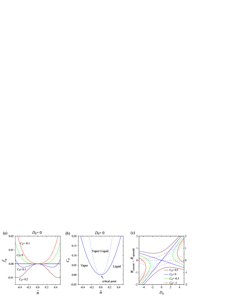
Figure 1: Coexistence of vapor and liquid phases if not considering the solid state. (a) The free energy density of uniform phase as a function of $\bar{n}$ at different $C_{0}$ ($=\epsilon-1$). (b) The $C_{0}$-$\bar{n}$ phase diagram for vapor and liquid states, where the boundary of vapor-liquid coexistence is plotted as solid lines and the spinodal line is plotted as dashed. $D_{0}=0$ is set in both (a) and (b). (c) The density of vapor-liquid coexistence ($\bar{n}_{\rm coexist}$, solid curves) or the spinodal density ($\bar{n}_{\rm spinodal}$, dashed curves) as a function of $D_{0}$ at different values of $C_{0}$. Other parameters are $B_{0}=0$ and $E_{0}=-6$.

In the rescaled original PFC model Eq. (2), we have $B_{0}=D_{0}=0$, $C_{0}=\epsilon-1$, and the temperature-related parameter $\epsilon$ is usually assumed to be small Elder and Grant (2004); Elder et al. (2007). In that case, the $f_{\rm u}(\bar{n})$ curve is convex, and thus there exists only one single phase under any density or pressure. In other words, vapor-liquid coexistence is absent under small $\epsilon$. However, when we extend the parameter region to large $\epsilon$, vapor-liquid coexistence actually occurs based on Eq. (4) without considering the solid state. Some sample curves of $f_{\rm u}(\bar{n})$ near $C_{0}=0$ are plotted in Fig. 1(a), which shows a double-well free energy when $C_{0}$ is positive, i.e., in the regime of $\epsilon>1$. The corresponding phase diagram with vapor-liquid coexistence is given in Fig. 1(b), where the critical point locates at $\bar{n}=0$, $C_{0}=0$ ($\epsilon=1$). Below the critical point, vapor and liquid are indistinguishable and there is no vapor-liquid coexistence. Above the critical point, vapor-liquid coexistence occurs and the coexistence regime expands with increasing $C_{0}$. Note that this result applies in the absence of solid phase which could become more stable in this parameter regime in the original PFC model.

The vapor-liquid coexistence is affected by the cubic term with nonzero $D_{0}$. Applying the common tangent rule on $f_{\rm u}(\bar{n})$ in Eq. (4), values of $\bar{n}$ for the vapor and liquid phases in coexistence are given by

$$\bar{n}_{\rm coexist}=\frac{-D_{0}\pm\sqrt{3D_{0}^{2}-6C_{0}E_{0}}}{E_{0}}.$$ (5)

The spinodal densities are determined by $\partial^{2}f_{\rm u}/\partial{\bar{n}}^{2}=0$, yielding

$$\bar{n}_{\rm spinodal}=\frac{-D_{0}\pm\sqrt{D_{0}^{2}-2C_{0}E_{0}}}{E_{0}}.$$ (6)

The corresponding results are plotted in Fig. 1(c) as a function of $D_{0}$. Introducing $D_{0}$ expands the region of vapor-liquid coexistence. For example, in the absence of $D_{0}$ the coexistence occurs only when $C_{0}>0$; in contrast, as shown in Fig. 1(c) with $E_{0}=-6$, at $D_{0}=\pm 3.46$ the coexistence regions is expanded to $C_{0}>-1$, i.e., to smaller values of $\epsilon$ within the scope of original PFC model.

In short, the above analysis indicates that the vapor-liquid coexistence can be realized within the PFC framework of a single density order parameter when $D_{0}^{2}>2C_{0}E_{0}$ (with $E_{0}<0$), under either large enough $C_{0}$ (or $\epsilon$) or large enough $|D_{0}|$.

III.2 Conditions for vapor-liquid-solid transitions

With the knowledge of vapor-liquid coexistence given above, we now explore the way to realize vapor-liquid-solid transitions. To simplify the problem and facilitate theoretical analysis, we adopt a one-mode approximation for $n(\mathbf{r})$ of periodic solid phases. For a one-dimensional (1D) stripe phase with amplitude $A$ and wave number $q$,

$$n(\mathbf{r})=\bar{n}+A\left(e^{iqx}+\textrm{c.c.}\right).$$ (7)

where “c.c.” represents complex conjugate. Substituting it into Eq. (3) yields the corresponding free energy density

$$f_{\rm stripe}\left(q,A;\bar{n}\right)=-B_{0}\bar{n}-\frac{1}{2}C_{0}\bar{n}^{2}-\frac{1}{6}D_{0}\bar{n}^{3}-\frac{1}{24}E_{0}\bar{n}^{4}$$

$$\quad-\left[\left(C_{0}-C_{2}q^{2}+C_{4}q^{4}\right)+\frac{1}{3}\left(3D_{0}-2D_{11}q^{2}\right)\bar{n}\right.$$

$$\quad\left.+\frac{1}{12}\left(6E_{0}+E_{1122}q^{4}\right)\bar{n}^{2}\right]A^{2}-\frac{1}{4}\left(E_{0}+E_{1122}q^{4}\right)A^{4}.$$

(8)

Note that for simplicity, here we assume $C_{6}=0$ in the free energy as the presence of $C_{6}$ term would not affect the basics of vapor-liquid-solid transition sequence. The specific role played by nonzero $C_{6}$ will be discussed separately at the beginning of Sec. IV.1. Similarly, for a 2D hexagonal or triangular phase the density field is expanded as

$$n(\mathbf{r})=\bar{n}+A\sum_{\mathbf{q}}\left(e^{i\mathbf{q}\cdot\mathbf{r}}+\textrm{c.c.}\right),$$ (9)

where the basic wave vectors $\mathbf{q}=q(1,0)$, $q(1/2,\sqrt{3}/2)$, and $q(1/2,-\sqrt{3}/2)$. The free energy density is then written by

$$f_{\rm hex}\left(q,A;\bar{n}\right)=-B_{0}\bar{n}-\frac{1}{2}C_{0}\bar{n}^{2}-\frac{1}{6}D_{0}\bar{n}^{3}-\frac{1}{24}E_{0}\bar{n}^{4}$$

$$\quad-3\left[\left(C_{0}-C_{2}q^{2}+C_{4}q^{4}\right)+\frac{1}{3}\left(3D_{0}-2D_{11}q^{2}\right)\bar{n}\right.$$

$$\qquad\quad\left.+\frac{1}{12}\left(6E_{0}+E_{1122}q^{4}\right)\bar{n}^{2}\right]A^{2}$$

$$\quad-\left[2\left(D_{0}-D_{11}q^{2}\right)+\left(2E_{0}+E_{1122}q^{4}\right)\bar{n}\right]A^{3}$$

$$\quad-\frac{15}{4}\left(E_{0}+E_{1122}q^{4}\right)A^{4}.$$ (10)

The equilibrium state is determined by minimizing the free energy density, i.e., $\min_{q,A}f(q,A;\bar{n})$ via $\partial f/\partial q=0$ and $\partial f/\partial A=0$. The corresponding results of equilibrium free energy density for stripe and hexagonal phases are plotted in Fig. 2 as a function of $\bar{n}$.

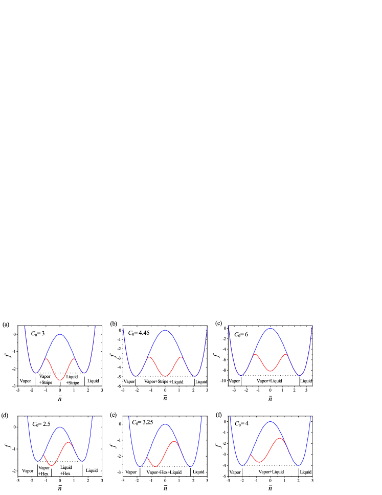
Figure 2: Equilibrium free energy density of uniform (blue) and solid (red) phases as a function of $\bar{n}$ at different values of $C_{0}$ in one-mode approximation, where the solid phase is of (a)–(c) 1D stripe or (d)–(f) 2D hexagonal (Hex) symmetry. The parameters used are $B_{0}=C_{6}=D_{0}=D_{11}=E_{1122}=0$, $C_{2}=-2$, $C_{4}=-1$, and $E_{0}=-6$.

The first row of Eq. (8) or Eq. (10) is identical to that of the uniform phase, either liquid or vapor, given in Eq. (4). To identify the conditions for achieving the vapor-liquid-solid transition sequence as $\bar{n}$ increases, in the following we consider the linear instability of the supercooled or supersaturated uniform phase with respect to the formation of the crystalline state, which is determined by the $A^{2}$ term in Eqs. (8) and (10), both being proportional to

$$\alpha(q,\bar{n})=- \left[\left(C_{0}-C_{2}q^{2}+C_{4}q^{4}\right)+\frac{1}{3}\left(3D_{0}-2D_{11}q^{2}\right)\bar{n}\right.$$ (11)

$$\left.+\frac{1}{12}\left(6E_{0}+E_{1122}q^{4}\right)\bar{n}^{2}\right].$$

When $\alpha<0$, a uniform liquid or vapor phase is linearly unstable under infinitesimal fluctuations and will crystallize spontaneously. To find the minimum of $\alpha$ with respect to $q$, we solve $\partial\alpha/\partial q=0$, leading to

$$q^{2}=\left\{\begin{array}[]{cc}\frac{6C_{2}+4D_{11}\bar{n}}{12C_{4}+E_{1122}{\bar{n}}^{2}},&{\rm if~{}}3C_{2}+2D_{11}\bar{n}<0,\\ 0,&{\rm if~{}}3C_{2}+2D_{11}\bar{n}\geq 0,\end{array}\right.$$ (12)

where $12C_{4}+E_{1122}{\bar{n}}^{2}<0$ is required to prevent the divergence at large $q$ as can be obtained from Eq. (11). Substituting Eq. (12) into Eq. (11) yields

$$\alpha(\bar{n})=-\left(C_{0}+D_{0}\bar{n}+\frac{1}{2}E_{0}\bar{n}^{2}\right)+\frac{\left(3C_{2}+2D_{11}\bar{n}\right)^{2}}{3\left(12C_{4}+E_{1122}{\bar{n}}^{2}\right)},$$ (13)

for $3C_{2}+2D_{11}\bar{n}<0$.

If $D_{11}=E_{1122}=0$ as in the original PFC model, we have $q^{2}={C_{2}}/{2C_{4}}$ which is independent of $\bar{n}$, and $C_{2}<0$ is needed to enable solid phases. Defining the supercooling or supersaturating density for the occurrence of linear instability by $\alpha(\bar{n})=0$, we have

$$\bar{n}_{\rm supercool}^{({\rm o})}=\frac{-D_{0}\pm\sqrt{D_{0}^{2}-2E_{0}\left(C_{0}-{C_{2}^{2}}/{4C_{4}}\right)}}{E_{0}}.$$ (14)

A solid phase would be more stable than a uniform phase (vapor or liquid) when $\bar{n}$ lies in between the two values of $\bar{n}^{({\rm o})}_{\rm supercool}$. Comparing Eq. (14) with Eqs. (5) and (6), it is clear that the midpoint of two $\bar{n}^{({\rm o})}_{\rm supercool}$ coincides with that of $\bar{n}_{\rm coexist}$ or $\bar{n}_{\rm spinodal}$ for vapor-liquid phases. Therefore, the stability regime of solid phase is expected to locate in between those of vapor and liquid, and the phase transition sequence is thus vapor-solid-liquid with the increase of density, consistent with the results of free energy density curves given in Fig. 2 for both 1D and 2D systems. The vapor-solid-liquid coexistence (corresponding to the triple point in phase diagram) can be realized via adjusting model parameters appropriately, as shown in Figs. 2(b) and 2(e). In this case, the density of solid is smaller than that of liquid, mimicking the unusual property of ice vs. water but not the behavior of most other materials. The above analysis hence demonstrates that it is impossible to describe the usual vapor-liquid-solid transition sequence in the original PFC model with $D_{11}=E_{1122}=0$.

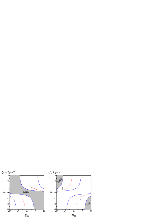
Figure 3: Variation of $\bar{n}_{\rm supercool}$ with $D_{11}$. Calculations are based on Eq. (15) shown as solid curves. The dashed lines correspond to $3C_{2}+2D_{11}\bar{n}=0$, while arrows point to the region of $3C_{2}+2D_{11}\bar{n}<0$. Regions for solid phase are shown in shadow. The parameters used are $B_{0}=C_{6}=D_{0}=E_{1122}=C_{0}=0$, $C_{4}=-1$, $E_{0}=-6$, and (a) $C_{2}=-2$, (b) $C_{2}=2$.

To achieve the usual vapor-liquid-solid transition sequence, we need to consider the effect of nonzero $D_{11}$. When $E_{1122}=0$, $\alpha(\bar{n})$ in Eq. (13) keeps its quadratic form of $\bar{n}$ and the linearly unstable condition of $\alpha(\bar{n})=0$ is still solvable analytically, yielding

$$\bar{n}_{\rm supercool}=\frac{-\left(D_{0}-\frac{C_{2}D_{11}}{3C_{4}}\right)\pm\sqrt{\left(D_{0}-\frac{C_{2}D_{11}}{3C_{4}}\right)^{2}-2\left(E_{0}-\frac{2D_{11}^{2}}{9C_{4}}\right)\left(C_{0}-\frac{C_{2}^{2}}{4C_{4}}\right)}}{E_{0}-\frac{2D_{11}^{2}}{9C_{4}}}.$$ (15)

Now the midpoint of two $\bar{n}_{\rm supercool}$ values does not coincide with that of $\bar{n}_{\rm coexist}$ or $\bar{n}_{\rm spinodal}$ anymore. More importantly, when the quadratic coefficient of $\alpha(\bar{n})$ in Eq. (13), i.e., $-{E_{0}}/{2}+{D_{11}^{2}}/{9C_{4}}$, is negative, the solid phase is more stable than the vapor or liquid uniform phase for $\bar{n}$ lying outside the range confined by the two $\bar{n}_{\rm supercool}$ values, but not in between them as before. This makes it possible to tune the phase stability parameters such that the density of solid would be higher than that of liquid, i.e., to realize the usual vapor-liquid-solid transition sequence. Some examples are illustrated in Fig. 3, where $C_{0}$ is set as 0 to approach the vapor-liquid coexistence, and $D_{0}=0$ is assigned by properly choosing the reference state so that vapor and liquid phases locate at opposite sides of $\bar{n}=0$ in the parameter space. In such a case, a vapor-liquid-solid transition sequence requires the solid phase to be on the positive side of $\bar{n}$. However, for $C_{2}=-2$ as used in most PFC models, the stability regime for solid always contains the point $\bar{n}=0$ [see Fig. 3(a)]; i.e., at $\bar{n}=0$ the solid state is more stable than the uniform phase. This can be easily verified from Eqs. (12) and (13) which show that $q^{2}>0$ and $\alpha(\bar{n})<0$ always hold at $\bar{n}=0$ for any $C_{0}\geq 0$ (which is necessary for vapor-liquid coexistence when $D_{0}=0$; see Sec. III.1), $C_{2}<0$, and $C_{4}<0$. It is noted that based on Eq. (12), $3C_{2}+2D_{11}\bar{n}<0$ is needed for the appearance of solid state, giving $C_{2}<0$ in the absence of $D_{11}$ as in previous PFC models. Conversely, with the introducing of nonzero $D_{11}$, $C_{2}<0$ is no longer obligatory (see also Appendix A). When $C_{2}=2$ [Fig. 3(b)], in the $D_{11}$-$\bar{n}$ diagram the stability regime for solid phase shrinks as compared to the case of $C_{2}=-2$, and locates at large enough $|D_{11}|$. Importantly, the solid phase is not stable near $\bar{n}=0$, leaving space for vapor-liquid coexistence to occur. As seen in Fig. 3(b), for small enough negative $D_{11}$ the density of solid is higher than that of uniform (vapor or liquid) phase as desired.

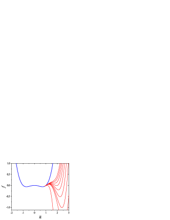
Figure 4: Equilibrium free energy density of uniform (blue) and stripe (red) phases as a function of $\bar{n}$ in one-mode approximation, for various values of $E_{1122}$. Result of uniform phase is not affected by $E_{1122}$, while for stripes the value of free energy density increases with the decrease of $E_{1122}$, i.e., $E_{1122}=0,-0.22,-0.24,-0.26,-0.28,-0.30,-0.32,-0.34,-0.36$ (red curves, from bottom to top). Other parameters are $B_{0}=C_{6}=D_{0}=0$, $C_{0}=0.5$, $C_{2}=2$, $C_{4}=-1$, $E_{0}=-6$, and $D_{11}=-8$.

The existence of proper vapor-liquid-solid transitions also requires the contribution of the $E_{1122}$ term. The reason is that although nonzero $D_{11}$ enables the stabilization of solid phase at density $\bar{n}$ larger than that of vapor and liquid phases, it overstabilizes the solid phase at very large $\bar{n}$. Take the stripe phase as an example, for which the free energy density at $E_{1122}=0$ is

$$f_{\rm stripe}(\bar{n})=-B_{0}\bar{n}-\frac{1}{2}C_{0}\bar{n}^{2}-\frac{1}{6}D_{0}\bar{n}^{3}-\frac{1}{24}E_{0}\bar{n}^{4}$$

$$+\frac{1}{E_{0}}\left[\frac{(3C_{2}+2D_{11}\bar{n})^{2}}{18C_{4}}-\left(C_{0}+D_{0}\bar{n}+\frac{1}{2}E_{0}\bar{n}^{2}\right)\right]^{2},$$ (16)

when $3C_{2}+2D_{11}\bar{n}<0$. The value of $f_{\rm stripe}(\bar{n})$ is dominated by the $\bar{n}^{4}$ terms when $\bar{n}\gg 1$. To prevent $f_{\rm stripe}\rightarrow-\infty$, it is required that

$$-\frac{1}{24}E_{0}+\frac{1}{E_{0}}\left[\frac{2D^{2}_{11}}{9C_{4}}-\frac{E_{0}}{2}\right]^{2}>0,$$ (17)

which however is incompatible with the condition of $-E_{0}/2+D_{11}^{2}/9C_{4}<0$ for the occurrence of vapor-liquid-solid transition sequence as discussed above. Therefore, a negative $E_{1122}$ is necessary to remedy this, as demonstrated in Fig. 4 which shows the increase of $f_{\rm stripe}$ and the avoidance of divergence as $E_{1122}$ becomes more negative.

In the next section we will conduct numerical calculations beyond one-mode approximation to achieve the three-phase coexistence and transition, based on the above theoretical analyses and the conditions identified for the realization of proper vapor-liquid-solid transitions.

IV Numerical results

Numerical calculations are conducted through the use of the time-evolution equation

$$\frac{\partial n}{\partial t}=\nabla^{2}\frac{\delta\mathcal{F}[n]}{\delta n},$$ (18)

which describes the conserved dynamics of density variation field $n(\mathbf{r},t)$. Given Eq. (3) for the free energy functional $\mathcal{F}$ of this model, the above dynamic equation is of the explicit form

$$\frac{\partial n}{\partial t} =\nabla^{2}\Biglb\{-\left(C_{0}+C_{2}\nabla^{2}+C_{4}\nabla^{4}+C_{6}\nabla^{6}\right)n$$ (19)

$$-\frac{1}{2}D_{0}n^{2}-\frac{1}{6}D_{11}\left(2n\nabla^{2}n+\nabla^{2}n^{2}\right)$$

$$-\frac{1}{6}E_{0}n^{3}-\frac{1}{12}E_{1122}\left[n(\nabla^{2}n)^{2}+\nabla^{2}(n^{2}\nabla^{2}n)\right]\Bigrb\}.$$

It is essentially governed by the diffusive, relaxational dynamics, and the system free energy decreases with time $t$ continuously until it reaches an equilibrium or steady state.

IV.1 Vapor-liquid-solid coexistence and phase diagrams

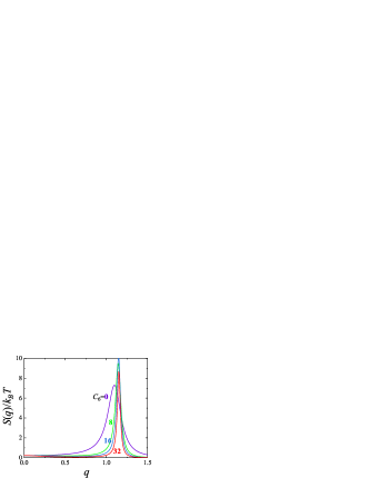
Figure 5: The fluid-state structure factor $S(q)$ at different values of $C_{6}$, evaluated from the analytic result derived in Appendix A. The curves are plotted with four sets of parameters, including $(C_{6},C_{2},C_{4})=(0,-10.6,-2.88)$, $(8,3.63,18.5)$, $(16,17.8,39.8)$, and $(32,46.3,82.5)$, with other parameters $C_{0}=-5.75$, $D_{0}=-9$, $E_{0}=-6$, $D_{11}=-34.2$, $E_{1122}=-52.1$, and $\bar{n}=-0.15$ remaining the same for each set. Each parameter set would lead to a state of vapor-liquid-solid coexistence under one-mode approximation of 2D hexagonal structure when $\bar{n}_{\rm vapor}=-2.5$, $\bar{n}_{\rm liquid}=-0.5$, $\bar{n}_{\rm solid}=0$, and $A=0.2$. As $C_{6}$ increases the peak position of $S(q)$ approaches the value $q=2/\sqrt{3}$ used in one-mode approximation.

Our above analyses have demonstrated that the free-energy functional Eq. (3) with $C_{6}=0$ is sufficient in obtaining the vapor-liquid-solid transitions under one-mode approximation. However, when solving the full PFC model via e.g., the dynamical Eq. (18), higher-order modes play a non-neglectable role and could cause undesired disturbances on the phase behavior. To enhance the dynamical stability of the one-mode-like solutions, we introduce the nonzero $C_{6}$ term into the two-point direct correlation, which can be used to control the degree of contributions from high-order modes on system properties. An example is given in Fig. 5, showing some sample results of equilibrium fluid-state structure factor $S(q)$ (as derived in Appendix A) for different values of $C_{6}$, each of which corresponds to a set of model parameters giving vapor-liquid-solid coexistence. These results indicate that contributions from high-order modes can be effectively suppressed at large $C_{6}$.

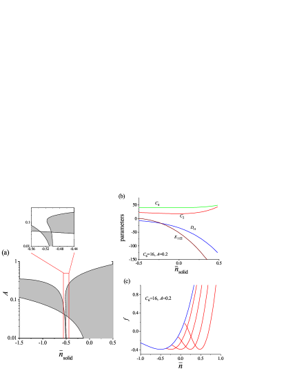
Figure 6: The broad range of model parameters yielding three-phase coexistence, under the condition of fixed values of $B_{0}=-1.875$, $C_{0}=-5.75$, $D_{0}=-9$, and $E_{0}=-6$ such that vapor-liquid coexistence occurs at $\bar{n}_{\rm vapor}=-2.5$ and $\bar{n}_{\rm liquid}=-0.5$. (a) Values of solid-phase coexistence density $\bar{n}_{\rm solid}$ and one-mode amplitude $A$ for 2D hexagonal phase that can lead to existence of solutions for vapor-liquid-solid or vapor-solid-liquid coexistence [across all possible combinations of $(C_{2},C_{4},D_{11},E_{1122})$], as indicated by the shaded region. The results are generated for $C_{6}=16$, with very similar outcomes for other choices of $C_{6}>0$. (b) The allowed values of parameter set $(C_{2},C_{4},D_{11},E_{1122})$ to achieve three-phase coexistence at different $\bar{n}_{\rm solid}$ when $C_{6}=16$ and $A=0.2$. (c) The free energy density curves of liquid (blue) and solid (red) phases corresponding to four of the parameter sets in (b) that give $\bar{n}_{\rm solid}=-0.25,0,0.25,0.5$, respectively. The vapor-phase free energy density (not shown here) is minimized at $\bar{n}=-2.5$ that forms a common tangent with these liquid- and solid-phase curves. The procedure of calculations under one-mode approximation is given in Appendix B.

With the introduction of nonzero $C_{6}$, we can identify a broad range of parameters that lead to vapor-liquid-solid coexistence in the new PFC model developed here. The general procedure for identifying the corresponding model parameters are described in Appendix B, which needs to be combined with some analytic conditions derived above in Sec. III in the absence of $C_{6}$ (particularly $D_{0}^{2}>2C_{0}E_{0}$, $D_{11}<0$, and $E_{1122}<0$). Numerical calculations are needed even in one-mode approximation, with some results presented in Fig. 6. Without loss of generality, in this example we fix the parameters $C_{0}=-5.75$, $D_{0}=-9$, and $E_{0}=-6$ so that vapor-liquid coexistence is found at $\bar{n}_{\rm vapor}=-2.5$ and $\bar{n}_{\rm liquid}=-0.5$ from Eq. (5). We then search for all the possible values of $C_{2}$, $C_{4}$, $D_{11}$, and $E_{1122}$ that give the solution of three-phase coexistence. Results in Fig. 6(a) indicates that the solution exists across a broad range of solid-phase coexistence density $\bar{n}_{\rm solid}$ and amplitude $A$. [It is interesting to note that in addition to vapor-liquid-solid coexistence (with $\bar{n}_{\rm vapor}<\bar{n}_{\rm liquid}<\bar{n}_{\rm solid}$), the parameter range for the unusual vapor-solid-liquid coexistence (with $\bar{n}_{\rm vapor}<\bar{n}_{\rm solid}<\bar{n}_{\rm liquid}$) can also be identified in this model, as seen in the part of $-1.5\leq\bar{n}_{\rm solid}<-0.5$ in Fig. 6(a).] In other words, at any specific $\bar{n}_{\rm solid}$ within this range the associated values of parameter set $(C_{2},C_{4},D_{11},E_{1122})$ can be found to achieve three-phase coexistence [see Fig. 6(b)]. This continuous adjustability of model parameters is demonstrated in an example of Fig. 6(c), where $\bar{n}_{\rm solid}$ is pre-selected from $-0.25$ to $0.50$ and for each of them we can always identify the corresponding combination values of model parameters [given in Fig. 6(b)] to obtain vapor-liquid-solid coexistence.

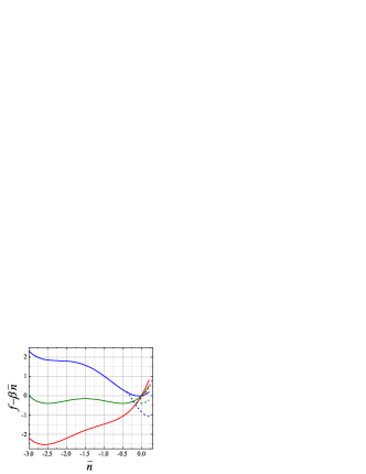
Figure 7: Free energy density profiles of uniform (solid curves) and 2D hexagonal (dashed) phases at different temperatures $\Delta T=-0.514$ (blue), $\Delta T=0$ (green), and $\Delta T=0.486$ (red), using model parameters listed in Table 1. Results are obtained from numerical solution of the full dynamical Eq. (18). Here all the free energy density curves have been tilted by a factor of $-\beta\bar{n}$ with $\beta=2.596$ for a better illustration.

Table 1: Model parameters used in numerical calculations of vapor-liquid-solid transitions. $\Delta T=0$ corresponds to the triple point temperature.

$B_{0}$	$C_{0}$	$C_{2}$	$C_{4}$	$C_{6}$	$D_{0}$	$D_{11}$	$E_{0}$	$E_{1122}$
$-4.5-3\Delta T$	$-5.764-\Delta T$	$17.8+2\Delta T$	$39.8-\Delta T$	$16$	$-9$	$-34.2$	$-6$	$-52.1$

To obtain accurate values of the solid-phase equilibrium free energy beyond one-mode approximation, we have numerically solved the full dynamical Eq. (18) using a single unit cell with periodic boundary conditions, and calculated the free energy density of its equilibrium, steady state. The initial density field $n(\mathbf{r},t=0)$ is set up either from the one-mode solution or from the existing simulation result of close parameter values. In addition, the numerical grid spacings $\Delta x$ and $\Delta y$ are varied to determine the equilibrium wave number and thus lattice constant from the minimum point of the corresponding free energy density obtained from simulations at each $\bar{n}$ and temperature. The resulting equilibrium free energy density for solid phase is then lower than that of one-mode approximation (although by a very small degree due to the effect of nonzero $C_{6}$ term), and we can slightly adjust the model parameters to achieve the desired phase stability and coexistence.

All the model parameters identified and used in the following full-model numerical calculations are summarized in Table 1, where $C_{0}$, $C_{2}$, and $C_{4}$ are set to be dependent on an effective temperature $\Delta T$ for the coexistence among vapor, liquid, and solid phases (with $\Delta T=0$ being the triple point temperature). Parameter $B_{0}$ for the linear term of the free energy functional is also set as temperature dependent, to produce the proper property of pressure (see below). Examples of the resulting equilibrium profiles of free energy density $f(\bar{n})$ are given in Fig. 7, at three different effective temperatures. At low temperature ($\Delta T=-0.514$) both vapor-liquid and vapor-solid coexistence can be identified from the $f$-$\bar{n}$ curves through the common tangent construction, while increasing temperature to $\Delta T=0$ brings the system to a vapor-liquid-solid coexistence as determined by the common tangent of the vapor, liquid, and solid free energy curves. Further increasing the temperature ($\Delta T=0.486$) excludes vapor-solid coexistence while the separate vapor-liquid and liquid-solid coexistence still remains. At high enough temperature, only liquid-solid coexistence can be found. All these results are consistent with the well-known behavior of the three phases.

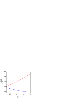
Figure 8: Saturation vapor pressure at vapor-liquid coexistence as a function of temperature $\Delta T$. Upper red line: $B_{0}=-4.5-3\Delta T$ as set in Table 1; Bottom blue line: $B_{0}=0$.

The pressure $P$ is also determined by $f(\bar{n})$. In the PFC approach, the quantitative result of pressure depends on the physical interpretation of the density variation field $n$ used in the model Wang et al. (2018c). Here we adopt the interpretation that $n=(\rho-\rho_{0})/\rho_{0}$, where $\rho$ is the atomic number density and $\rho_{0}$ is a reference-state density. The total number of particles $N$ in the system is kept constant under any deformations of volume $V$, with $N=\int\rho d\mathbf{r}=\bar{\rho}V=\rho_{0}(\bar{n}+1)V$ where $\bar{\rho}$ is the spatial average of $\rho(\mathbf{r})$, leading to ${\partial\bar{n}}/{\partial V}=-N/(\rho_{0}V^{2})$. The equilibrium pressure is hence given by (noting $\mathcal{F}=fV$)

$$P=-\frac{\partial\mathcal{F}}{\partial V}=-f-V\frac{\partial f}{\partial\bar{n}}\frac{\partial\bar{n}}{\partial V}=-f+(\bar{n}+1)\frac{\partial f}{\partial\bar{n}}.$$ (20)

For a solid phase, numerical solution of the full PFC model is required to calculate this pressure $P$ through $f(\bar{n})$ of the equilibrium state. For uniform vapor or liquid phase, we can obtain the analytic expression of $P$ based on Eq. (4) for $f$, i.e.,

$$P_{\rm uniform} = -B_{0}-\frac{1}{2}C_{0}\left(\bar{n}^{2}+2\bar{n}\right)$$ (21)

$$-\frac{1}{6}D_{0}\left(2\bar{n}^{3}+3\bar{n}^{2}\right)-\frac{1}{24}E_{0}\left(3\bar{n}^{4}+4\bar{n}^{3}\right).$$

The saturation vapor pressure $P_{\rm u}^{\rm(SVP)}$ at vapor-liquid coexistence can be calculated by substituting Eq. (5) for coexistence density into Eq. (21). Some results are depicted in Fig. 8, showing the important role of $B_{0}$ on the temperature dependence of $P$. When $B_{0}=0$ and using values given in Table 1 for other parameters (bottom blue line in Fig. 8) ${P}_{\rm u}^{\rm(SVP)}$ decreases with the increase of temperature $\Delta T$, a behavior that is not correct. The correct temperature-increasing behavior of ${P}_{\rm u}^{\rm(SVP)}$ is obtained only when $B_{0}$ is set to be temperature dependent, such as $B_{0}=-4.5-3\Delta T$ given in Table 1 (upper red line in Fig. 8).

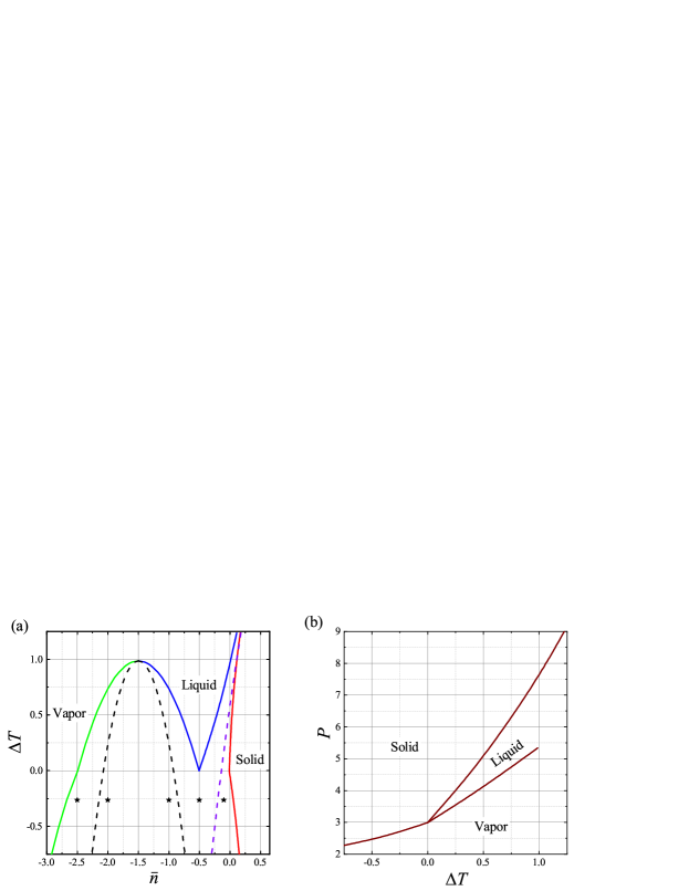
Figure 9: Vapor-liquid-solid phase diagrams calculated numerically from the full PFC model, where the solid state is of 2D hexagonal phase. (a) Temperature-density phase diagram, where the phase boundaries for vapor, liquid, and solid states are plotted in green, blue, and red, respectively, the vapor-liquid spinodal is plotted as the black dashed curve, and the linear instability of the homogeneous state is indicated by the purple dashed line. Star symbols refer to the 5 parameter locations used in our numerical simulations shown in Fig. 11. (b) Temperature-pressure phase diagram. The model parameters listed in Table 1 are used.

Based on these information of $f$ and $P$, we compute the vapor-liquid-solid phase diagrams of the full PFC model using the parameters listed in Table 1, as shown in Fig. 9. Following the procedure described above, at each temperature $\Delta T$ the equilibrium free energy density $f$ for solid phase is evaluated numerically from simulations of single unit cell for different values of $\bar{n}$ (see some examples in Fig. 7). The resulting $f$-$\bar{n}$ relations are then used in the common tangent construction described in Appendix B to obtain the temperature-density phase diagram presented in Fig. 9(a). At the same time the corresponding pressure value at phase coexistence densities can be determined from Eqs. (20) and (21) for each $\Delta T$, giving the temperature-pressure phase diagram in Fig. 9(b).

These calculated phase diagrams possess expected properties of vapor-liquid-solid transitions and coexistence. For example, for vapor-solid coexistence at low temperatures (with $\Delta T<0$) the vapor coexistence density increases with temperature but the solid one decreases, while for liquid-solid coexistence at intermediate and high temperatures ($\Delta T>0$), both liquid and solid coexistence densities increase with temperature [see Fig. 9(a)]. In addition, both the triple point and critical point are obtained in the temperature-pressure phase diagram [Fig. 9(b)]. We have conducted some numerical simulations to verify the phase behavior identified here, with sample results given below in Sec. IV.3. All these results are consistent with experimental phase diagrams of pure materials (e.g., argon) and those of previous computer simulations (such as the Lennard-Jones system).

IV.2 Equilibrium lattice spacing: Effects of thermal expansion and pressure

A drawback of the previous PFC models is the lack of lattice thermal expansion effect, and also the lack of a study of effects of pressure $P$ and density $\bar{n}$ on the lattice constant. For example, in the original PFC model the equilibrium wave number in one-mode approximation is given by $q_{\rm eq}=\sqrt{{C_{2}}/{2C_{4}}}$, which is independent of $\bar{n}$, $P$, and temperature as $C_{2}$ and $C_{4}$ were assumed to be temperature independent constants Elder et al. (2007). In this model $C_{2}$ and $C_{4}$ are set to be dependent on the temperature (see Table 1), and with the incorporation of high-order correlations in the model (related to three- and four-point interactions), $q_{\rm eq}$ is affected by $\bar{n}$ and hence pressure $P$ via $D_{11}$ and $E_{1122}$ terms [see e.g., Eq. (12)]. Therefore, both thermal expansion and pressure effects have been incorporated in this three-phase PFC model.

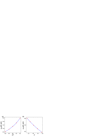
Figure 10: Thermal and pressure effects on lattice constant. (a) Thermal expansion of equilibrium lattice spacing $a_{\rm eq}=2\pi/q_{\rm eq}$ under a constant pressure $P=3.87$. (b) The pressure-induced variation of $a_{\rm eq}$ under a constant temperature $\Delta T=0$. Parameters in Table 1 for 2D hexagonal phase are used in numerical calculations.

Results of numerical calculations of equilibrium lattice spacing $a_{\rm eq}$ for 2D hexagonal structure are shown in Fig. 10, subjected to variations of temperature and pressure. During the process of equilibrium free energy density and phase diagram calculations described above, $q_{\rm eq}$ has already been determined through free energy minimization at each $\bar{n}$ and $\Delta T$, yielding the corresponding lattice constant $a_{\rm eq}=2\pi/q_{\rm eq}$. For each value of average density $\bar{n}$, pressure $P$ is calculated numerically based on Eq. (20). Figure 10(a) shows that at a constant value of $P$, $a_{\rm eq}$ increases with larger temperature $\Delta T$, indicating a behavior with positive thermal expansion coefficient as in a majority of materials. In addition, when temperature $\Delta T$ is kept constant while $P$ is varied, Fig. 10(b) shows that $a_{\rm eq}$ decreases with increasing $P$, consistent with the compression effect of pressure on the lattice.

IV.3 Dynamical simulations

We have conducted dynamical simulations based on Eq. (18) using the model parameters listed in Table 1, to examine the above results of vapor-liquid-solid transitions and coexistence. Our focus is on the regime involving vapor phase at and below the triple point temperature in the phase diagram (i.e., $\Delta T\leq 0$), with some sample results presented in Figs. 11 and 12.

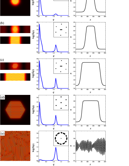
Figure 11: Sample results from PFC simulations at $\Delta T=-0.264$, corresponding to the locations marked in the phase diagram of Fig. 9(a) below the triple point temperature. They include five characteristic cases for which the initial configuration is set up as a crystalline nucleus of $\bar{n}=0.1$ and grid size $48\times 48$ embedded in a uniform phase of (a) $\bar{n}=-2.5$, (b) $\bar{n}=-2$, (c) $\bar{n}=-1$, and (d) $\bar{n}=-0.5$, or by (e) a random initial condition of $\bar{n}=-0.1$ in the whole system. Left column: Spatial structure at the steady state of phase coexistence [(a)–(d)] or at the late stage of the polycrystalline state (e). An early-stage configuration having liquid-vapor phase separation is also shown in (b) and (c) for initial $\bar{n}$ within the spinodal. The brighter (darker) regions correspond to higher (lower) values of density field $n$. Middle column: The corresponding circularly averaged structure factor, with the diffraction pattern shown as inset. Right column: The $y$-averaged density of the final state across the grid points along the $x$ direction.

Figure 11 shows five typical scenarios of structural evolution and phase coexistence, with the corresponding parameter values of the initial uniform phase indicated in the temperature-density phase diagram of Fig. 9(a) at $\Delta T=-0.264$. The simulations in Figs. 11(a)–11(d) were initialized from a spatially homogeneous state of density $\bar{n}_{\rm uniform}$, with a solid seed of 2D hexagonal structure of $\bar{n}=0.1$ placed at the center, while a random initial condition of $\bar{n}=-0.1$ was set in the whole system of Fig. 11(e). In addition to the spatial structure configurations, the circularly averaged structure factor, diffraction pattern, and the $y$-averaged density profile along the $x$ direction are presented in Fig. 11 for the final state of simulations. The final state in Figs. 11(a)–11(d) corresponds to equilibrium two-phase coexistence, for which the structure factor shows two peaks, one at small wave number $q$ as caused by the vapor or liquid region while the other corresponding to the hexagonal lattice inside the solid grain. For the polycrystalline state in Fig. 11(e), the small-$q$ peak of the structure factor can be attributed to the existence of multiple grains in the sample.

When the initial value of average density $\bar{n}$ locates between the vapor phase boundary and the spinodal curve of the phase diagram, such as $\bar{n}_{\rm uniform}=-2.5$ in the case of Fig. 11(a), no vapor-liquid separation occurs in the initially homogeneous region and the system equilibrium state is characterized by the coexistence between vapor phase and a stabilized faceted solid grain, as expected. For Fig. 11(b) with $\bar{n}_{\rm uniform}=-2.0$ and Fig. 11(c) with $\bar{n}_{\rm uniform}=-1.0$ that are close to two opposite sides of the spinodal boundary, similar results of vapor-solid state are obtained, although with larger equilibrium solid region appearing in the latter case, consistent with the lever rule. Both values of $\bar{n}_{\rm uniform}$ locate within the spinodal regime, so that vapor-liquid phase separation occurs spontaneously at the early stage of system evolution, as can be seen in the top panels of the left column in Figs. 11(b) and 11(c). The liquid-phase region shrinks with time and eventually disappears, while the initial solid grain grows and saturates, leading to an equilibrium state with vapor-solid coexistence as shown in the bottom panels of the left column (see also the averaged density profile given in the right column). When initially $\bar{n}_{\rm uniform}=-0.5$, lying between the spinodal curve and linear instability line, the final equilibrium state shows a coexistence between liquid region and the embedded faceted solid grain, as seen in Fig. 11(d). Finally, at $\bar{n}=-0.1$ which is beyond the linear instability line, the initial homogeneous state is linearly unstable, leading to the spontaneous formation of the crystalline structure across the system which evolves to a polycrystalline configuration shown in Fig. 11(e). The system consists of various topological defects including dislocations and grain boundaries, resulting in the spatial oscillations of the $y$-averaged density profile across the $x$ direction as presented in the bottom-right panel of the figure.

To further illustrate the phenomenon of vapor-liquid-solid coexistence, we simulate a system of 2D slab configuration at $\Delta T=0$, starting with half of the slab occupied by solid phase with $\bar{n}=-0.012$ while the other half by a homogeneous state with $\bar{n}=-1.5$ (at the middle of the spinodal regime), as shown in Fig. 12(a). Through spinodal decomposition, the system spontaneously evolves into a mixture of vapor, liquid, and solid [Fig. 12(b)]. The resulting smoothed average density [Fig. 12(c)] closely matches to that of the equilibrium phase diagram in Fig. 9(a), i.e., $\bar{n}=-2.493$, $-0.507$, and $-0.012$ for vapor, liquid, and solid phases, respectively. It is noted that in this simulated system the solid region is actually of higher energy due to the existing of interfaces and nonzero interfacial energy, and thus shrinks slowly with time during the system evolution.

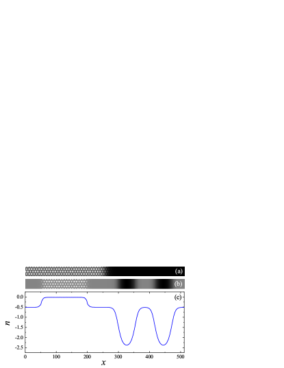
Figure 12: PFC simulation results of vapor-liquid-solid coexistence at $\Delta T=0$, using the model parameters given in Table 1. (a) The initial state with half of system in solid (with $\bar{n}=-0.012$) and the other half in a uniform state (with $\bar{n}=-1.5$). (b) The time-evolving state with vapor-liquid-solid coexistence. (c) The corresponding $y$-averaged density along the $x$ direction.

V Conclusions

We have introduced a new PFC model with high-order correlations featuring three- and four-body interactions to examine the transitions and coexistence among vapor, liquid, and crystalline solid phases within a single continuum density-field description, without making any pre-assumptions other than the basic requirement of system rotational invariance. The advantage of this model has been demonstrated in terms of its simple form, genericness and flexibility of parameter choices in achieving three-phase coexistence and transitions, including both vapor-liquid-solid and the unusual vapor-solid-liquid transition sequence. Through both theoretical analysis and numerical computation, the conditions of phase coexistence are identified, as well as temperature-density and temperature-pressure phase diagrams incorporating vapor-liquid-solid triple point and vapor-liquid critical point, which qualitatively agree with the well-known results of previous experiments and atomistic simulations. Various scenarios of vapor-solid, liquid-solid, and vapor-liquid-solid coexistence, vapor-liquid phase separation, and structural evolution are verified through dynamical simulations of the model.

In addition, several material properties missing in the previous PFC models, including temperature dependence of saturation vapor pressure, thermal expansion, and compression effect of pressure on lattice constant, can be well produced in this model, with outcomes consistent with the known results. Thus the approach developed here, which well describes the vapor-liquid-solid phase behaviors and the corresponding material properties, can serve as a valuable tool for modeling the material growth and evolution processes including both vapor- and liquid-based and vapor-liquid-solid growth.

Appendix A Structure factor of the homogeneous state

The structure factor for homogeneous fluids can be determined from a linear analysis of the dynamic equation governing the density field $n$. In the homogeneous fluid state the density can be decomposed as $n(\mathbf{r},t)=\bar{n}+\delta n(\mathbf{r},t)$ with a small fluctuation $\delta n(\mathbf{r},t)$. Linearizing the dynamical Eq. (18), in Fourier space we get

$$\frac{\partial\delta\hat{n}_{\mathbf{q}}}{\partial t}=-\gamma_{\mathbf{q}}\delta\hat{n}_{\mathbf{q}}+\hat{\eta}_{\mathbf{q}},$$ (22)

where $\delta\hat{n}_{\mathbf{q}}$ is the Fourier transform of $\delta n$, and

$$\gamma_{\mathbf{q}} = {q}^{2}\left[-\left({C_{0}}+{\bar{n}}{{D}_{0}}+\frac{1}{2}\bar{n}^{2}E_{0}\right)+\left(C_{2}+\frac{2}{3}{\bar{n}}{D_{11}}\right){q}^{2}\right.$$ (23)

$$\left.-\left(C_{4}+\frac{1}{12}\bar{n}^{2}E_{1122}\right){q}^{4}+C_{6}{q}^{6}\right].$$

Here we have introduced a noise term $\hat{\eta}_{\mathbf{q}}$, which is the Fourier component of the noise field $\eta$ satisfying $\langle\eta(\mathbf{r},t)\rangle=0$ and $\langle\eta(\mathbf{r},t)\eta(\mathbf{r}^{\prime},t^{\prime})\rangle=-2k_{B}T\nabla^{2}\delta(\mathbf{r}-\mathbf{r}^{\prime})\delta(t-t^{\prime})$; thus $\langle\hat{\eta}_{\mathbf{q}}(t)\hat{\eta}^{*}_{\mathbf{q}^{\prime}}(t^{\prime})\rangle=2k_{B}Tq^{2}\delta(\mathbf{q}-\mathbf{q}^{\prime})\delta(t-t^{\prime})$.

Following the procedure given in Ref. Elder and Grant (2004), we obtain the solution of Eq. (22) as

$$\delta\hat{n}_{\mathbf{q}}(t)=e^{-\gamma_{\mathbf{q}}t}\delta\hat{n}_{\mathbf{q}}(0)+e^{-\gamma_{\mathbf{q}}t}\int_{0}^{t}dse^{\gamma_{\mathbf{q}}s}\hat{\eta}_{\mathbf{q}}(s),$$ (24)

and calculate the fluid-state structure factor by

$$S(\mathbf{q},t) = \left\langle\left|\delta\hat{n}_{\mathbf{q}}\right|^{2}\right\rangle=\left\langle\left|\delta\hat{n}_{\mathbf{q}}\delta\hat{n}_{-\mathbf{q}}\right|\right\rangle$$ (25)

$$= e^{-2\gamma_{\mathbf{q}}t}\left\langle\left|\delta\hat{n}_{\mathbf{q}}(0)\right|^{2}\right\rangle$$

$$+e^{-2\gamma_{\mathbf{q}}t}\int_{0}^{t}{dsds^{\prime}e^{\gamma_{\mathbf{q}}(s+s^{\prime})}\left\langle\hat{\eta}_{\mathbf{q}}(s)\hat{\eta}_{-{\mathbf{q}}}(s^{\prime})\right\rangle}$$

$$= e^{-2\gamma_{\mathbf{q}}t}S({\mathbf{q}},0)+\frac{k_{B}Tq^{2}}{\gamma_{\mathbf{q}}}\left(1-e^{-2\gamma_{\mathbf{q}}t}\right).$$

The equilibrium fluid-state structure factor is defined by $S(\mathbf{q})=S(\mathbf{q},t\to\infty)$, yielding

$$S(q)=\frac{k_{B}Tq^{2}}{\gamma_{\mathbf{q}}}=\frac{k_{B}T}{-\left(C_{0}^{\prime}-C_{2}^{\prime}q^{2}+C_{4}^{\prime}q^{4}-C_{6}^{\prime}q^{6}\right)},$$ (26)

where

$$C_{0}^{\prime}=C_{0}+\bar{n}D_{0}+\frac{1}{2}\bar{n}^{2}E_{0},\qquad C_{2}^{\prime}=C_{2}+\frac{2}{3}\bar{n}D_{11},$$

$$C_{4}^{\prime}=C_{4}+\frac{1}{12}\bar{n}^{2}E_{1122},\qquad C_{6}^{\prime}=C_{6}.$$ (27)

Appendix B Phase coexistence and model parameters selection

In this appendix we show the procedure of identifying three-phase coexistence in this PFC model and how to choose the corresponding model parameters. According to the common tangent rule, in the equilibrium state the coexistence between any two phases is determined by equal chemical potential $\mu_{n}$ and equal pressure $P_{n}$, i.e.,

$$\left.\frac{\partial f}{\partial\bar{n}}\right|_{1}=\left.\frac{\partial f}{\partial\bar{n}}\right|_{2}=\mu_{n}$$

$$f_{1}-\mu_{n}{\bar{n}}_{1}=f_{2}-\mu_{n}{\bar{n}}_{2}=-P_{n},$$ (28)

giving coexistence densities ${\bar{n}}_{1}$ and ${\bar{n}}_{2}$ for phase 1 and 2, respectively. [Note that $P_{n}=P-\mu_{n}$ if compared to Eq. (20) for pressure $P$ obtained through density $\bar{\rho}$.]

In this PFC model the free energy density for uniform phase, either vapor ($f_{\rm vapor}$) or liquid ($f_{\rm liquid}$), is known from Eq. (4), and the exact solution of coexistence densities $\bar{n}_{\rm vapor}$ and $\bar{n}_{\rm liquid}$ is given by Eq. (5). Thus from Eq. (28) we can get the value of $\mu_{n}=(f_{\rm liquid}-f_{\rm vapor})/(\bar{n}_{\rm liquid}-\bar{n}_{\rm vapor})$ from vapor-liquid coexistence, and the following conditions governing the vapor-liquid-solid coexistence

$$\left.\frac{\partial{f_{\rm solid}}}{{\partial\bar{n}}}\right|_{\bar{n}_{\rm solid}}=\mu_{n}=\frac{f_{\rm liquid}-f_{\rm vapor}}{\bar{n}_{\rm liquid}-\bar{n}_{\rm vapor}},$$ (29)

$$f_{\rm solid}=f_{\rm liquid}+\frac{(\bar{n}_{\rm solid}-\bar{n}_{\rm liquid})(f_{\rm liquid}-f_{\rm vapor})}{\bar{n}_{\rm liquid}-\bar{n}_{\rm vapor}}.$$ (30)

For the full model, the solid-state free energy density $f_{\rm solid}$ is calculated from the steady state of the numerical solution of dynamical Eq. (18) for a single-crystal unit cell (see Sec. IV.1), while phase coexistence is determined by the common tangent construction described above, given the known results of coexisting vapor and liquid phases in Eqs. (4) and (5).

There are many adjustable parameters in the model, including $B_{0}$, $C_{j=0,2,4,6}$, $D_{0}$, $E_{0}$, $D_{11}$, and $E_{1122}$. For simplicity, we first fix the values of $B_{0}$, $C_{0}$, $D_{0}$, and $E_{0}$ so that the properties of vapor and liquid phases are pre-determined, such as the coexistence densities $\bar{n}_{\rm vapor}$ and $\bar{n}_{\rm liquid}$, the resulting $f_{\rm vapor}$ and $f_{\rm liquid}$, and saturation vapor pressure (see Fig. 8). Value of $C_{6}$ is also chosen in advance based on its effect on high-order modes (see e.g., Fig. 5). We then have only four parameters $C_{2}$, $C_{4}$, $D_{11}$, and $E_{1122}$ left to be determined, to satisfy the conditions of three-phase coexistence.

We first follow this procedure with the use of one-mode approximation for solid phase to determine all the model parameters, and then slightly adjust them (to account for the discrepancy between one-mode and full-model results) to obtain phase coexistence and phase diagrams from numerical calculations of the full PFC model. The one-mode free energy density $f_{\rm solid}$ is given by Eq. (8) for 1D stripe and by Eq. (10) for 2D hexagonal phase, respectively. Its equilibrium state with minimum free energy is obtained by solving

$$\frac{\partial{f_{\rm solid}}}{{\partial A}}=0,\qquad\frac{\partial{f_{\rm solid}}}{{\partial q}}=0.$$ (31)

We thus have four equations in Eqs. (29)–(31) to be solved numerically for seven unknown variables $C_{2}$, $C_{4}$, $D_{11}$, $E_{1122}$, $A$, $q$, and $\bar{n}_{\rm solid}$ in one-mode approximation. To identify the allowed values of model parameters $C_{2}$, $C_{4}$, $D_{11}$, and $E_{1122}$ yielding three-phase coexistence, we solve these equations under specific values of $A$, $\bar{n}_{\rm solid}$, and $q$ (fixed as $2/\sqrt{3}$ here in 2D one-mode expansion at the triple point) that can lead to the existence of solution. The corresponding results are presented in Fig. 6.