Forced-exploration free Strategies for Unimodal Bandits

Abstract

We consider a multi-armed bandit problem specified by a set of Gaussian or Bernoulli distributions endowed with a unimodal structure. Although this problem has been addressed in the literature (Combes and Proutiere, 2014), the state-of-the-art algorithms for such structure make appear a forced-exploration mechanism. We introduce IMED-UB, the first forced-exploration free strategy that exploits the unimodal-structure, by adapting to this setting the Indexed Minimum Empirical Divergence (IMED) strategy introduced by Honda and Takemura (2015). This strategy is proven optimal. We then derive KLUCB-UB, a KLUCB version of IMED-UB, which is also proven optimal. Owing to our proof technique, we are further able to provide a concise finite-time analysis of both strategies in an unified way. Numerical experiments show that both IMED-UB and KLUCB-UB perform similarly in practice and outperform the state-of-the-art algorithms.

Keywords: Structured Bandits, Indexed Minimum Empirical Divergence, Optimal Strategy

1 Introduction

The multi-armed bandit problem is a popular framework to formalize sequential decision making problems. It was first introduced in the context of medical trials (Thompson, 1933, 1935) and later formalized by Robbins (1952): A bandit is specified by a set of unknown probability distributions $\nu\!=\!(\nu_{a})_{a\in\mathcal{A}}$ with means $(\mu_{a})_{a\in\mathcal{A}}$. At each time $t\!\in\!\mathbb{N}$, the learner chooses an arm $a_{t}\!\in\!\mathcal{A}$, based only on the past, the learner then receives and observes a reward $X_{t}$, conditionally independent, sampled according to $\nu_{a_{t}}$. The goal of the learner is to maximize the expected sum of rewards received over time (up to some unknown horizon $T$), or equivalently minimize the regret with respect to the strategy constantly receiving the highest mean reward

$$R(\nu,T)=\mathbb{E}_{\nu}\!\left[\sum_{t=1}^{T}\mu^{\star}-X_{t}\right]\text{ where }\mu^{\star}=\max_{a\in\mathcal{A}}\mu_{a}\,.$$

Both means and distributions are unknown, which makes the problem non trivial, and the learner only knows that $\nu\!\in\!\mathcal{D}$ where $\mathcal{D}$ is a given set of bandit configurations. This problem received increased attention in the middle of the $20^{\text{th}}$ century, and the seminal paper Lai and Robbins (1985) established the first lower bound on the cumulative regret, showing that designing a strategy that is optimal uniformly over a given set of configurations $\mathcal{D}$ comes with a price. The study of the lower performance bounds in multi-armed bandits successfully lead to the development of asymptotically optimal strategies for specific configuration sets, such as the KLUCB strategy (Lai, 1987; Cappé et al., 2013; Maillard, 2018) for exponential families, or alternatively the DMED and IMED strategies from Honda and Takemura (2011, 2015). The lower bounds from Lai and Robbins (1985), later extended by Burnetas and Katehakis (1997) did not cover all possible configurations, and in particular structured configuration sets were not handled until Agrawal et al. (1989) and then Graves and Lai (1997) established generic lower bounds. Here, structure refers to the fact that pulling an arm may reveals information that enables to refine estimation of other arms. Unfortunately, designing numerical efficient strategies that are provably optimal remains a challenge for many structures.

Structured configurations.

Motivated by the growing popularity of bandits in a number of industrial and societal application domains, the study of structured configuration sets has received increasing attention over the last few years: The linear bandit problem is one typical illustration (Abbasi-Yadkori et al., 2011; Srinivas et al., 2010; Durand et al., 2017), for which the linear structure considerably modifies the achievable lower bound, see Lattimore and Szepesvari (2017). The study of a unimodal structure naturally appears in many contexts, e.g. single-peak preference economics, voting theory or wireless communications, and has been first considered in Yu and Mannor (2011) from a bandit perspective, then in Combes and Proutiere (2014) providing an explicit lower bound together with a strategy exploiting this specific structure. Other structures include Lipschitz bandits Magureanu et al. (2014), and we refer to the manuscript Magureanu (2018) for other examples, such as cascading bandits that are useful in the context of recommender systems. In Combes et al. (2017), a generic strategy is introduced called OSSB (Optimal Structured Stochastic Bandit), stepping the path towards generic multi-armed bandit strategies that are adaptive to a given structure.

Unimodal-structure.

In this paper, we provide novel regret minimization results related to the following structure. We assume a unimodal structure similar to that considered in Yu and Mannor (2011) and Combes and Proutiere (2014). That is, there exists an undirected graph $G\!=\!(\mathcal{A},E)$ whose vertices are arms $\mathcal{A}$, and whose edges $E$ characterize a partial order among means $(\mu_{a})_{a\in\mathcal{A}}$. This partial order is assumed unknown to the learner. We assume that there exists a unique optimal arm $a^{\star}\!=\!\mathop{\mathrm{argmax}}_{a\in\mathcal{A}}\mu_{a}$ and that for all sub-optimal arm $a\!\neq\!a^{\star}$, there exists a path $P_{a}\!=\!(a_{1}\!=\!a,\dots,a_{\ell_{a}}\!=\!a^{\star})\!\in\!\mathcal{A}^{\ell_{a}}$ of length $\ell_{a}\!\geqslant\!2$ such that for all $i\!\in\![1,\ell_{a}-1]$, $(a_{i},a_{i+1})\in E$ and $\mu_{a_{i}}<\mu_{a_{i+1}}$. Lastly, we assume that $\nu\!\subset\!\mathcal{P}\!\coloneqq\!\left\{p(\mu),\mu\!\in\!\Theta\right\}$, where $p(\mu)$ is an exponential-family distribution probability with density $f(\cdot,\mu)$ with respect to some positive measure $\lambda$ on $\mathbb{R}$ and mean $\mu\!\in\!\Theta\!\subset\!\mathbb{R}$. $\mathcal{P}$ is assumed to be known to the learner. Thus, for all $a\!\in\!\mathcal{A}$ we have $\nu_{a}\!=\!p(\mu_{a})$. We denote by $\mathcal{D}_{(\mathcal{P},G)}$ or simply $\mathcal{D}$ the structured set of such unimodal-bandit distributions characterized by $\left(\mathcal{P},G\right)$. In the following, we assume that $\mathcal{P}$ is either the set of real Gaussian distributions with means in $\mathbb{R}$ and variance $1$ or the set of Bernouilli distributions with means in $(0,1)$.

Goal.

A key contribution in the study of unimodal bandits is the work Combes and Proutiere (2014), where the authors establish lower confidence bounds on the regret for the unimodal structure, and introduce an asymptotically optimal strategy called OSUB. One may then consider that unimodal bandits are solved. Unfortunately, a closer look at the proposed approach reveals that the considered strategy forces some arms to be played (this is different than what is called forced exploration in structured bandits; it is rather a forced exploitation scheme). In this paper, our goal is to introduce alternative strategies to OSUB, that do not use any such forcing scheme, but consider variants of the pseudo-index induced by the lower bound analysis. Whether or not forcing mechanisms are desirable features is currently still under debate in the community; by providing the first strategy without any requirement for forcing in a structured bandit setup, we show that such mechanisms are not always required, which we believe opens an interesting avenue of research.

Contributions.

In this paper, we first revisit the Indexed Minimum Empirical Divergence (IMED) strategy from Honda and Takemura (2011) introduced for unstructured multi-armed bandits, and adapt it to the unimodal-structured setting. We introduce in Section 3 the IMED-UB strategy that is limited to the pulling of the current best arm or their no more than $d$ nearest arms at each time step, with $d$ the maximum degree of nodes in $G$. Being constructed from IMED, IMED-UB does not require any optimization procedure and does not separate exploration from exploitation rounds. IMED-UB appears to be a local strategy. Motivated by practical considerations, under the assumption that $G$ is a tree, when the number of arms $\left|\mathcal{A}\right|$ becomes large, we further develop d-IMED-UB, an algorithm that behaves like IMED-UB while resorting to a dichotomic second order exploration over all nodes of the graph. This helps quickly identify the best arm $a^{\star}$ within a large set of arms $\mathcal{A}$ by empirical considerations. We also introduce for completeness the KLUCB-UB strategy, that is similar to IMED-UB, but inspired from UCB strategies. We prove in Theorem 9 that IMED-UB, d-IMED-UB and KLUCB-UB are asymptotically optimal strategies that do not require forcing scheme. Furthermore, our unified finite time analysis shows that IMED-UB and KLUCB-UB are closely related. Furthermore, these novel strategies significantly outperform OSUB in practice. This is confirmed by numerical illustrations on synthetic data. We believe that the construction of these algorithms together with the proof techniques developed in this paper are of independent interest for the bandit community.

Notations.

Let $\nu\!\in\!\mathcal{D}$. Let $\mu^{\star}\!=\!\max_{a\in\mathcal{A}}\mu_{a}$ be the optimal mean and $a^{\star}\!=\!\mathop{\mathrm{argmax}}_{a\in\mathcal{A}}{\mu_{a}}$ be the optimal arm of $\nu$. We define for an arm $a\!\in\!\mathcal{A}$ its sub-optimality gap $\Delta_{a}\!=\!\mu^{\star}\!-\!\mu_{a}$. Considering an horizon $T\!\geqslant\!1$, thanks to the chain rule we can rewrite the regret as follows:

$$R(\nu,T)=\sum_{a\in\mathcal{A}}\Delta_{a}\,\mathbb{E}_{\nu}\big{[}N_{a}(T)\big{]}\,,$$ (1)

where $N_{a}(t)\!=\!\sum_{s=1}^{t}\mathbb{I}_{\left\{a_{s}=a\right\}}$ is the number of pulls of arm $a$ at time $t$.

2 Regret Lower bound

In this subsection, we recall for completeness the known lower bound on the regret when we assume a unimodal structure. In order to obtain non trivial lower bound we consider strategies that are consistent (aka uniformly-good).

Definition 1 (Consistent strategy)

A strategy is consistent on $\mathcal{D}$ if for all configuration $\nu\in\mathcal{D}$, for all sub-optimal arm $a$, for all $\alpha>0$,

$$\lim\limits_{T\rightarrow\infty}\mathbb{E}_{\nu}\!\left[\dfrac{N_{a}(T)}{T^{\alpha}}\right]=0\,.$$

We can derive from the notion of consistency an asymptotic lower bound on the regret, see Combes and Proutiere (2014). To this end, we introduce $\mathcal{V}_{a}\!=\!\left\{a^{\prime}\in\mathcal{A}:\ (a,a^{\prime})\in E\right\}$ to denote the neighbourhood of an arm $a\in\mathcal{A}$.

Proposition 2 (Lower bounds on the regret)

Let us consider a consistent strategy. Then, for all configuration $\nu\!\in\!\mathcal{D}$, it must be that

$$\liminf\limits_{T\rightarrow\infty}\dfrac{R(\nu,T)}{\log(T)}\geqslant c(\nu):=\sum_{a\in\mathcal{V}_{a^{\star}}}\dfrac{\Delta_{a}}{\text{KL}\!\left(\mu_{a}\right.\!\!\left|\mu^{\star}\right)}\,,$$

where $\text{KL}\!\left(\mu\right.\!\!\left|\mu^{\prime}\right)\!=\!\int_{\mathbb{R}}\!\log\!\left(f(x,\mu)/f(x,\mu^{\prime})\right)\!f(x,\mu)\lambda(\mathrm{d}x)$ denotes the Kullback-Leibler divergence between $\nu\!=\!p(\mu)$ and $\nu^{\prime}\!=\!p(\mu^{\prime})$, for $\mu,\mu^{\prime}\!\in\!\Theta$.

Remark 3

The quantity $c(\nu)$ is a fully explicit function of $\nu$ (it does not require solving any optimization problem) for some set of distributions $\nu$ (see Remark 4). This useful property no longer holds in general for arbitrary structures. Also, it is noticeable that $c(\nu)$ does not involve all the sub-optimal arms but only the ones in $\mathcal{V}_{a^{\star}}$. This indicates that sub-optimal arms outside $\mathcal{V}_{a^{\star}}$ are sampled $o(\log(T))$, which contrasts with the unstructured stochastic multi-armed bandits. See Combes and Proutiere (2014) for further insights.

Remark 4

For Gaussian distributions (variance $\sigma^{2}\!=\!1$), we assume $\lambda$ to be the Lebesgue measure, $\Theta\!=\!\mathbb{R}$, and for $\mu\!\in\!\mathbb{R}$, $f(\cdot,\mu)\!=:x\!\in\!\mathbb{R}\mapsto(\sqrt{2\pi})^{-1}e^{-(x-\mu)^{2}\!/2}$. Then for all $\mu,\mu^{\prime}\!\in\!\mathbb{R}$, $\text{KL}\!\left(\mu\right.\!\!\left|\mu^{\prime}\right)\!=\!(\mu^{\prime}\!-\!\mu)^{2}\!/2$. For Bernoulli distributions, a possible setting is to assume $\lambda=\delta_{0}+\delta_{1}$ (with $\delta_{0},\delta_{1}$ Dirac measures), $\Theta\!=\!(0,1)$ and for $\mu\!\in\!\Theta$, $f(\cdot,\mu)\!=:x\!\in\!\left\{0,1\right\}\mapsto\mu^{x}(1-\mu)^{1-x}$. Then for all $\mu,\mu^{\prime}\!\in\![0,1]$, $\text{KL}\!\left(\mu\right.\!\!\left|\mu^{\prime}\right)\!=\!\text{kl}\!\left(\mu\right.\!\!\left|\mu^{\prime}\right)$, where

$$\text{kl}\!\left(\mu\right.\!\!\left|\mu^{\prime}\right)\!\coloneqq\!\left\{\begin{array}[]{ll}\!\!\!0&\textnormal{if }\mu\!=\!\mu^{\prime},\\ \!\!\!+\infty&\textnormal{if }\mu\!<\!\mu^{\prime}\!=\!1,\\ \!\!\!\mu\log\!\left(\frac{\mu}{\mu^{\prime}}\right)+(1\!-\!\mu)\log\!\left(\frac{1\!-\!\mu}{1\!-\!\mu^{\prime}}\right)&\textnormal{otherwise},\\ \end{array}\right.$$

with the convention $0\!\times\!\log(0)\!=\!0$.

3 Forced-exploration free strategies for unimodal-structured bandits

We present in this section three novel strategies that both match the asymptotic lower bound of Proposition 2. Two of these strategies are inspired by the Indexed Minimum Empirical Divergence (IMED) proposed by Honda and Takemura (2011). The other one is based on Kullback–Leibler Upper Confidence Bounds (KLUCB), using insights from IMED. The general idea behind these algorithms is, following the intuition given by the lower bound, to narrow on the current best arm and its neighbourhood for pulling an arm at a given time step.

Notations.

The empirical mean of the rewards from the arm $a$ is denoted by ${{\widehat{\mu}}}_{a}(t)\!=\!\sum_{s=1}^{t}{\mathbb{I}_{\left\{a_{s}=a\right\}}X_{s}}/N_{a}(t)$ if $N_{a}(t)\!>\!0$, $0$ otherwise. We also denote by ${{\widehat{\mu}}}^{\star}(t)\!=\!\max_{a\in\mathcal{A}}{{\widehat{\mu}}}_{a}(t)$ and $\widehat{\mathcal{A}}^{\star}(t)\!=\!\mathop{\mathrm{argmax}}_{a\in\mathcal{A}}{{\widehat{\mu}}}_{a}(t)$ respectively the current best mean and the current set of optimal arms.

For convenience, we recall below the OSUB (Optimal sampling for Unimodal Bandits) strategy from Combes and Proutiere (2014).

Algorithm 1 OSUB

  Pull an arbitrary arm $a_{1}\in\mathcal{A}$

  for $t=1\dots T-1$ do

     Choose $\widehat{a}^{\star}_{t}\in\mathop{\mathrm{argmin}}\limits_{\widehat{a}^{\star}\in\widehat{\mathcal{A}}^{\star}(t)}N_{\widehat{a}^{\star}}(t)$ (chosen arbitrarily)

     Pull $a_{t+1}=\begin{cases}\widehat{a}^{\star}_{t}&\text{ if }\frac{L_{t}(\widehat{a}^{\star}_{t})-1}{d+1}\in\mathbb{N}\\ \mathop{\mathrm{argmax}}\limits_{a\in\mathcal{V}_{\widehat{a}^{\star}_{t}}}u_{a}(t)&\text{else}\end{cases}$

  end for

In Algorithm 1, for some numerical constant $c\!>\!0$, the index computed by OSUB strategy for arm $a\!\in\!\mathcal{A}$ and step $t\!\geqslant\!1$ is

$$u_{a}(t)\!=\!\sup\big{\{}u\!\geqslant\!{{\widehat{\mu}}}_{a}(t)\!:N_{a}(t)\text{KL}\!\left({{\widehat{\mu}}}_{a}(t)\right.\!\!\left|u\right)\!\leqslant\!f_{c}\!\left(L_{t}(\widehat{a}^{\star}_{t})\right),$$

where $L_{t}(a)\!=\!\sum_{t^{\prime}=1}^{t}\mathbb{I}_{\left\{\widehat{a}^{\star}_{t^{\prime}}=a\right\}}$ counts how many times arm $a$ was a leader (best empirical arm), $d$ is the maximum degree of nodes in $G$, and $f_{c}(\cdot)\!=\!\log(\cdot)\!+\!c\log\log(\cdot)$.

3.1 The IMED-UB strategy.

For all arm $a\!\in\!\mathcal{A}$ and time step $t\!\geqslant\!1$ we introduce the IMED index

$$I_{a}(t)=N_{a}(t)\,\text{KL}\!\left({{\widehat{\mu}}}_{a}(t)\right.\!\!\left|{{\widehat{\mu}}}^{\star}(t)\right)+\log\!\left(N_{a}(t)\right)\,,$$

with the convention $0\!\times\!\infty\!=\!0$. This index can be seen as a transportation cost for moving a sub-optimal arm to an optimal one plus an exploration term: the logarithm of the numbers of pulls. When an optimal arm is considered, the transportation cost is null and there is only the exploration part. Note that, as stated in Honda and Takemura (2011), $I_{a}(t)$ is an index in the weaker sense since it cannot be determined only by samples from the arm $a$ but also uses empirical means of current optimal arms. We define IMED-UB (Indexed Minimum Empirical Divergence for Unimodal Bandits), described in Algorithm 2, to be the strategy consisting of pulling an arm $a_{t}\!\in\!\left\{\widehat{a}^{\star}_{t}\right\}\!\cup\!\mathcal{V}_{\widehat{a}^{\star}_{t}}$ with minimum index at each time step $t$, where is $\widehat{a}^{\star}_{t}\!\in\!\mathop{\mathrm{argmin}}_{\widehat{a}^{\star}\in\widehat{\mathcal{A}}^{\star}(t)}N_{\widehat{a}^{\star}}(t)$ is a current best arm. This is a natural algorithm since the lower bound on the regret given in Proposition 2 involves only the arms in $\mathcal{V}_{a^{\star}}$, the neighbourhood of the arm $a^{\star}$ of maximal mean.

Algorithm 2 IMED-UB

  Pull an arbitrary arm $a_{1}\in\mathcal{A}$

  for $t=1\dots T-1$ do

     Choose $\widehat{a}^{\star}_{t}\in\mathop{\mathrm{argmin}}\limits_{\widehat{a}^{\star}\in\widehat{\mathcal{A}}^{\star}(t)}N_{\widehat{a}^{\star}}(t)$ (chosen arbitrarily)

     Pull $a_{t+1}\in\mathop{\mathrm{argmin}}\limits_{a\in\left\{\widehat{a}^{\star}_{t}\right\}\cup\mathcal{V}_{\widehat{a}^{\star}_{t}}}I_{a}(t)$ (chosen arbitrarily)

  end for

3.2 The KLUCB-UB strategy

For all arm $a\!\in\!\mathcal{A}$ and time step $t\!\geqslant\!1$ we introduce the following Upper Confidence Bound

$$U_{a}(t)\!=\!\max\!\left\{\begin{array}[]{l}u\geqslant{{\widehat{\mu}}}_{a}(t)\\ N_{a}(t)\text{KL}\!\left({{\widehat{\mu}}}_{a}(t)\right.\!\!\left|u\right)\!+\!\log\!\left(N_{a}(t)\right)\!\leqslant\!\log\!\left(N_{\widehat{a}_{t}^{\star}}(t)\right)\end{array}\right\}$$

with $\widehat{a}^{\star}_{t}\!\in\!\mathop{\mathrm{argmin}}\limits_{\widehat{a}^{\star}\in\widehat{\mathcal{A}}^{\star}(t)}\!N_{\widehat{a}^{\star}}(t)$.

By convention, we set $U_{a}(t)\!=\!{{\widehat{\mu}}}_{a}(t)$ if for $a\!\in\!\mathcal{A}$, $\log\!\left(N_{a}(t)\right)\!>\!\log\!\left(N_{\widehat{a}_{t}^{\star}}(t)\right)$.

Remark 5

A classical KLUCB strategy would replace the term $\log\!\left(N_{\widehat{a}_{t}^{\star}}(t)/N_{a}(t)\right)$ with $\log(t)$, and a KLUCB⁺ would use $\log(t/N_{a}(t))$. This is a simple yet crucial modification. Indeed, although this makes KLUCB-UB not an index strategy, this enables to get a more intrinsic strategy, to simplify the analysis and get improved numerical results.

As for IMED-UB and IMED, $U_{a}(t)$ is an index in a weaker sense since it cannot be determined only by samples from the arm $a$ but also uses numbers of pulls of current optimal arms. We define KLUCB-UB (Kullback-Leibler Upper Confidence Bounds for Unimodal Bandits) to be the strategy consisting of pulling an arm $a_{t}\!\in\!\left\{\widehat{a}^{\star}_{t}\right\}\cup\mathcal{V}_{\widehat{a}^{\star}_{t}}$ with maximum index at each time step $t$. This algorithm can be seen as a KLUCB version of the IMED-UB strategy.

Algorithm 3 KLUCB-UB

  Pull $a_{1}\in\mathcal{A}$ at random.

  for $t=1\dots T-1$ do

     Choose $\widehat{a}^{\star}_{t}\in\mathop{\mathrm{argmin}}\limits_{\widehat{a}^{\star}\in\widehat{\mathcal{A}}^{\star}(t)}N_{\widehat{a}^{\star}}(t)$ (chosen arbitrarily)

     Pull $a_{t+1}\in\mathop{\mathrm{argmax}}\limits_{a\in\left\{\widehat{a}^{\star}_{t}\right\}\cup\mathcal{V}_{\widehat{a}^{\star}_{t}}}U_{a}(t)$ (chosen arbitrarily)

  end for

Remark 6

IMED-UB does not require solving any optimization problem, unlike OSUB or KLUCB-UB. We believe this feature, inherited from IMED, makes it an especially appealing strategy. KLUCB-UB solves an optimization similar to that of the KLUCB strategy for unstructured bandits, and also related to the optimization used in OSUB from Combes and Proutiere (2014). The difference between KLUCB-UB and OSUB is that it does not use any forced exploitation.

3.3 The d-IMED-UB strategy for large set of arms

When the set of arms is large, a bad initialization of IMED-UB (that is, choose arm $a_{1}$ far from $a^{\star}$) comes with high initial regret. Indeed, IMED-UB does not allow to explore outside the neighbourhood $\mathcal{V}_{\widehat{a}^{\star}_{t}}$ of $\widehat{a}^{\star}_{t}$. When $\mathcal{A}$ is large compared to the neighbourhoods, this may generate a large burn-in phase. To overcome this practical limitation, it is natural to explore outside the neighbourhood of the current best arm. However, to be compatible with the lower bound on the regret stated in Proposition 2 such exploration must be asymptotically negligible. We now consider $\mathcal{G}$ to be a tree, and introduce d-IMED-UB, a strategy that trades-off between these two types of exploration. d-IMED-UB shares with IMED-UB the same exploitation criteria and explores if the index of the current best arm exceeds the indexes of arms in its neighbourhood. However, in exploration phase, d-IMED-UB runs an IMED type strategy to choose between exploring within or outside the neighbourhood of the current best arm. For all time step $t\!\geqslant\!1$, for all arm $a^{\prime}\!\in\!\mathcal{V}_{\widehat{a}^{\star}_{t}}$, for all arm $a\!\in\!\widehat{G}_{a^{\prime}}(t)$, where $G_{a^{\prime}}(t)$ denotes the sub-tree containing $a^{\prime}$ obtained by cutting edge $(a^{\prime},\widehat{a}^{\star}_{t})$, we define the second order IMED index relative to $a^{\prime}$, as

$$I_{a}^{(a^{\prime})}(t)=N_{a}(t)\,\text{KL}\!^{+}\!\!\left({{\widehat{\mu}}}_{a}(t)\right.\!\!\left|{{\widehat{\mu}}}_{a^{\prime}}(t)\right)+\log\!\left(N_{a}(t)\right)\,,$$

where $\text{KL}\!^{+}\!\!\left(\mu\right.\!\!\left|\mu^{\prime}\right)\!=\!\text{KL}\!\left(\mu\right.\!\!\left|\mu^{\prime}\right)$ if $\mu\!<\!\mu^{\prime}$, $0$ otherwise. At each exploration time step, d-IMED-UB pulls an arm in $\mathcal{S}_{t}$ with minimal secondary index relative to the arm $\underline{a}_{t}$ with current minimal index and belonging to the neighbourhood of the current best arm, where $\mathcal{S}_{t}$ is a sub-tree of $\widehat{G}_{\underline{a}_{t}}(t)$ dichotomously chosen that contains $\underline{a}_{t}$. We illustrate in Appendix E, a way to dynamically choose $\mathcal{S}_{t}$.

Remark 7

Assuming that $G$ is a tree ensures that for all $a^{\prime}\!\in\!\mathcal{V}_{a^{\star}}$, the nodes of $G_{a^{\prime}}$, the sub-tree containing $a^{\prime}$ obtained by cutting edge $(a^{\prime},a^{\star})$, induce a unimodal bandit configuration with optimal arm $a^{\prime}$. This specific property allows establishing the optimality of d-IMED-UB.

Algorithm 4 d-IMED-UB

  Pull an arbitrary arm $a_{1}\in\mathcal{A}$

  for $t=1\dots T-1$ do

     Choose $\widehat{a}^{\star}_{t}\in\mathop{\mathrm{argmin}}\limits_{\widehat{a}^{\star}\in\widehat{\mathcal{A}}^{\star}(t)}N_{\widehat{a}^{\star}}(t)$ (chosen arbitrarily)

     Choose $\underline{a}_{t}\in\mathop{\mathrm{argmin}}\limits_{a\in\left\{\widehat{a}^{\star}_{t}\right\}\cup\mathcal{V}_{\widehat{a}^{\star}_{t}}}I_{a}(t)$ (chosen arbitrarily)

     if $\underline{a}_{t}=\widehat{a}^{\star}_{t}$ then

        Pull $a_{t+1}=\underline{a}_{t}$

     else

        Pull $a_{t+1}\in\mathop{\mathrm{argmin}}\limits_{a\in\mathcal{S}_{t}}I^{(\underline{a}_{t})}_{a}(t)$

     end if

  end for

3.4 Asymptotic optimality of IMED-UB, d-IMED-UB and KLUCB-UB

In this section, we state the main theoretical result of this paper.

Theorem 8 (Upper bounds)

Let us consider a set of Gaussian or Bernoulli distributions $\nu\!\in\!\mathcal{D}$ and let $a^{\star}$ its optimal arm. Let $\mathcal{V}_{a^{\star}}$ be the sub-optimal arms in the neighbourhood of $a^{\star}$. Then under IMED-UB and KLUCB-UB strategies for all $0\!<\!\varepsilon\!<\!\varepsilon_{\nu}$, for all horizon time $T\!\geqslant\!1$, for all $a\!\in\!\mathcal{V}_{a^{\star}}$,

$$\mathbb{E}_{\nu}[N_{a}(T)]\leqslant\dfrac{1+\alpha_{\nu}(\varepsilon)}{\text{KL}\!\left(\mu_{a}\right.\!\!\left|\mu_{a^{\star}}\right)}\log(T)+d\left|\mathcal{A}\right|^{2}C_{\varepsilon}+1$$

and, for all $a\!\notin\!\left\{a^{\star}\right\}\!\cup\!\mathcal{V}_{a^{\star}}$,

$$\mathbb{E}_{\nu}[N_{a}(T)]\leqslant d\left|\mathcal{A}\right|^{2}C_{\varepsilon}+1\,,$$

where $d$ is the maximum degree of nodes in $G$, $\varepsilon_{\nu}\!=\!\min\left\{1\!-\!\mu^{\star},\,\min_{a\neq a^{\prime}}\left|\mu_{a}\!-\!\mu_{a^{\prime}}\right|\!/\!4\right\}$, $C_{\varepsilon}\!=\!34\log(1\!/\!\varepsilon)\varepsilon^{-6}$ and where $\alpha_{\nu}(\cdot)$ is a non-negative function depending only on $\nu$ such that $\lim\limits_{\varepsilon\to 0}\alpha_{\nu}(\varepsilon)\!=\!0$ (see Section 4.1 for more details).

Furthermore, if the considered graph is a tree, then under d-IMED-UB, for all horizon $T\!\geqslant\!1$, for all $a\in\mathcal{V}_{a^{\star}}$,

$$\mathbb{E}_{\nu}[N_{a}(T)]\leqslant\dfrac{1+\alpha_{\nu}(\varepsilon)}{\text{KL}\!\left(\mu_{a}\right.\!\!\left|\mu_{a^{\star}}\right)}\log(T)+d\left|\mathcal{A}\right|^{2}C_{\varepsilon}+1$$

and, for all $a\!\notin\!\left\{a^{\star}\right\}\!\cup\!\mathcal{V}_{a^{\star}}$,

$$\mathbb{E}_{\nu}\!\left[N_{a}(T)\right] \leqslant \dfrac{1+\alpha_{\nu}(\varepsilon)}{\min\limits_{\underline{a}\in\mathcal{V}_{a^{\star}}}\!\!\text{KL}\!\left(\mu_{a}\right.\!\!\left|\mu_{\underline{a}}\right)}\log\!\!\left(\!\dfrac{1+\alpha_{\nu}(\varepsilon)}{\min\limits_{\underline{a}\in\mathcal{V}_{a^{\star}}}\!\!\text{KL}\!\left(\mu_{\underline{a}}\right.\!\!\left|\mu_{a^{\star}}\!\right)}\!\log(T)\!\!\right)$$

$$+ d\left|\mathcal{A}\right|^{2}C_{\varepsilon}+1\,.$$

In particular one can note that the arms in the neighbourhood of the optimal one are pulled $\mathcal{O}\!\left(\log(T)\right)$ times while the other sub-optimal arms are pulled a finite number of times under IMED-UB and KLUCB-UB, and $\mathcal{O}\!\left(\log\!\log(T)\right)$ times under d-IMED-UB. This is coherent with the lower bound that only involves the neighbourhood of the best arm. More precisely, combining Theorem 8 and the chain rule (1) gives the asymptotic optimality of IMED-UB and KLUCB-UB with respect to the lower bound of Proposition 2.

Corollary 9 (Asymptotic optimality)

With the same notations as in Theorem 8 , then under IMED-UB and KLUCB-UB strategies

$$\limsup\limits_{T\rightarrow\infty}\dfrac{R(\nu,T)}{\log(T)}\leqslant c(\nu)=\sum\limits_{a\in\mathcal{V}_{a^{\star}}}\dfrac{\Delta_{a}}{\text{KL}\!\left(\mu_{a}\right.\!\!\left|\mu^{\star}\right)}\,.$$

If the considered graph is a tree, same result holds under d-IMED-UB strategy.

See respectively Section 4 and Appendix C for a finite time analysis of IMED-UB, d-IMED-UB and KLUCB-UB.

4 IMED-UB finite time analysis

At a high level, the key interesting step of the proof is to realize that the considered strategies imply empirical lower and empirical upper bounds on the numbers of pulls (see Lemma 10, Lemma 11 for IMED-UB). Then, based on concentration lemmas (see Section A.1), the strategy-based empirical lower bounds ensure the reliability of the estimators of interest (Lemma 14). This makes use of more classical arguments based on concentration of measure. Then, combining the reliability of these estimators with the obtained strategy-base empirical upper bounds, we obtain upper bounds on the average numbers of pulls (Theorem 8).

In this section, we only detail the finite time analysis of IMED-UB algorithm and defer those of d-IMED-UB and KLUCB-UB to the appendix, as it follows essentially the same steps. Indeed, we show that KLUCB and d-IMED-UB strategies imply empirical bounds (Lemmas 19,20, Lemmas 25,26) very similar to IMED-UB strategy . This inequalities are the cornerstone of the analysis. We believe that this general way of proceeding is of independent interest as it simplifies the proof steps.

4.1 Notations

Let us consider $\nu\!\in\!\mathcal{D}$ and let us denote by $a^{\star}$ its best arm. We recall that for all $a\!\in\!\mathcal{A}$, $\mathcal{V}_{a}\!=\!\left\{a^{\prime}\in\mathcal{A}:\ (a,a^{\prime})\in E\right\}$ is the neighbourhood of arm $a$ in graph $G\!=\!(\mathcal{A},E)$, and that

$$d=\max\limits_{a\in\mathcal{A}}\left|\mathcal{V}_{a}\right|,\ \varepsilon_{\nu}=\min\left\{1-\mu^{\star},\ \min\limits_{a\neq a^{\prime}}\dfrac{\left|\mu_{a}-\mu_{a^{\prime}}\right|}{4}\right\}\,.$$

Then, there exists a function $\alpha_{\nu}(\cdot)$ such that for all $a\neq a^{\prime}$, for all $0\!<\!\varepsilon\!<\!\varepsilon_{\nu}$,

$$\dfrac{\text{kl}\!\left(\mu_{a}\right.\!\!\left|\mu_{a^{\prime}}\right)}{1+\alpha_{\nu}(\varepsilon)}\leqslant\text{kl}\!\left(\mu_{a}+\varepsilon\right.\!\!\left|\mu_{a^{\prime}}-\varepsilon\right)\leqslant(1+\alpha_{\nu}(\varepsilon))\text{kl}\!\left(\mu_{a}\right.\!\!\left|\mu_{a^{\prime}}\right)$$

and $\lim\limits_{\varepsilon\downarrow 0}\downarrow\alpha_{\nu}(\varepsilon)=0$. For all studied strategy, at each time step $t\!\geqslant\!1$, $\widehat{a}^{\star}_{t}$ is arbitrarily chosen in $\mathop{\mathrm{argmin}}\limits_{a\in\widehat{\mathcal{A}}^{\star}(t)}N_{a}(t)$ where $\widehat{\mathcal{A}}^{\star}(t)\!=\!\mathop{\mathrm{argmax}}\limits_{a\in\mathcal{A}}{{\widehat{\mu}}}_{a}(t)$.

For all arms $a\!\in\!\mathcal{A}$ and $n\!\geqslant\!1$, we introduce the stopping times $\tau_{a,n}\!=\!\inf{\left\{t\!\geqslant\!1\!:N_{a}(t)\!=\!n\right\}}$ and define the empirical means corresponding to local times

$${{\widehat{\mu}}}_{a}^{n}=\dfrac{1}{n}\sum\limits_{m=1}^{n}X_{\tau_{a,m}}\,.$$

For a subset of times $\mathcal{E}\!\subset\!\left\{t\!\geqslant\!1\right\}$, we denote by $\mathcal{E}^{c}$ its complementary in $\left\{t\geqslant 1\right\}$.

4.2 Strategy-based empirical bounds

IMED-UB strategy implies inequalities between the indexes that can be rewritten as inequalities on the numbers of pulls. While lower bounds involving $\log(t)$ may be expected in view of the asymptotic regret bounds, we show lower bounds on the numbers of pulls involving instead $\log\!\left(N_{a_{t+1}}(t)\right)$, the logarithm of the number of pulls of the current chosen arm. We also provide upper bounds on $N_{a_{t+1}}(t)$ involving $\log(t)$.

We believe that establishing these empirical lower and upper bounds is a key element of our proof technique, that is of independent interest and not a priori restricted to the unimodal structure.

Lemma 10 (Empirical lower bounds)

Under IMED-UB, at each step time $t\!\geqslant\!1$, for all $a\!\in\!\mathcal{V}_{\widehat{a}_{t}^{\star}}$,

$$\log\!\left(N_{a_{t+1}}(t)\right)\leqslant N_{a}(t)\,\text{KL}\!\left({{\widehat{\mu}}}_{a}(t)\right.\!\!\left|{{\widehat{\mu}}}^{\star}(t)\right)+\log\!\left(N_{a}(t)\right)$$

and

$$N_{a_{t+1}}(t)\leqslant N_{\widehat{a}^{\star}_{t}}(t)\,.$$

Proof  For $a\!\in\!\mathcal{A}$, by definition, we have $I_{a}(t)\!=\!N_{a}(t)\text{KL}\!\left({{\widehat{\mu}}}_{a}(t)\right.\!\!\left|{{\widehat{\mu}}}^{\star}(t)\right)\!+\!\log\!\left(N_{a}(t)\right)$, hence

$$\log\!\left(N_{a}(t)\right)\leqslant I_{a}(t)\,.$$

This implies, since the arm with minimum index is pulled, $\log\!\left(N_{a_{t+1}}(t)\right)\!\leqslant\!I_{a_{t+1}}(t)\!=\!\min\limits_{a^{\prime}\in\left\{\widehat{a}^{\star}_{t}\right\}\!\cup\!\mathcal{V}_{\widehat{a}^{\star}_{t}}}I_{a^{\prime}}(t)\!\leqslant\!I_{\widehat{a}^{\star}_{t}}(t)\!=\!\log\!\left(N_{\widehat{a}^{\star}_{t}}(t)\right)$. By taking the $\exp(\cdot)$, the last inequality allows us to conclude.  

Lemma 11 (Empirical upper bounds)

Under IMED-UB at each step time $t\!\geqslant\!1$,

$$N_{a_{t+1}}(t)\,\text{KL}\!\left({{\widehat{\mu}}}_{a_{t+1}}(t)\right.\!\!\left|{{\widehat{\mu}}}^{\star}(t)\right)\leqslant\log(t)\,.$$

Proof  As above, by construction we have

$$I_{a_{t+1}}(t)\leqslant I_{\widehat{a}^{\star}_{t}}(t)\,.$$

It remains, to conclude, to note that

$$N_{a_{t+1}}(t)\text{KL}\!\left({{\widehat{\mu}}}_{a_{t+1}}(t)\right.\!\!\left|{{\widehat{\mu}}}^{\star}(t)\right)\leqslant I_{a_{t+1}}(t)\,,$$

and

$$I_{\widehat{a}^{\star}_{t}}(t)=\log(N_{\widehat{a}^{\star}_{t}}(t))\leqslant\log(t)\,.$$

 

4.3 Reliable current best arm and means

In this subsection, we consider the subset $\mathcal{T}_{\varepsilon}$ of times where everything is well behaved: The current best arm corresponds to the true one and the empirical means of the best arm and the current chosen arm are $\varepsilon$-accurate for $0\!<\!\varepsilon\!<\!\varepsilon_{\nu}$, that is

$$\mathcal{T}_{\varepsilon}\coloneqq\left\{\begin{array}[]{l}t\geqslant 1:\ \widehat{\mathcal{A}}^{\star}(t)=\left\{a^{\star}\right\}\\ \hskip 28.45274pt\forall a\in\left\{a^{\star},a_{t+1}\right\},\ \left|{{\widehat{\mu}}}_{a}(t)-\mu_{a}\right|<\varepsilon\end{array}\!\right\}\,.$$

We will show that its complementary set is finite on average. In order to prove this we decompose the set $\mathcal{T}_{\varepsilon}$ in the following way. Let $\mathcal{E}_{\varepsilon}$ be the set of times where the means are well estimated,

$$\mathcal{E}_{\varepsilon}\coloneqq\left\{t\geqslant 1:\ \forall a\!\in\!\widehat{\mathcal{A}}^{\star}\!(t)\!\cup\!\left\{a_{t+1}\right\},\ \left|{{\widehat{\mu}}}_{a}(t)-\mu_{a}\right|<\varepsilon\right\}\,,$$

and $\Lambda_{\varepsilon}$ the set of times where an arm that is not the current optimal neither pulled is underestimated

$$\Lambda_{\varepsilon}\!\coloneqq\!\!\left\{\begin{array}[]{l}t\!\geqslant\!1\!:\exists a\in\mathcal{V}_{\widehat{a}^{\star}_{t}}\!\setminus\!\left\{a_{t+1},\widehat{a}^{\star}_{t}\right\}\textnormal{ s.t. }{{\widehat{\mu}}}_{a}(t)\!<\!\mu_{a}\!-\!\varepsilon\textnormal{ and}\\ \log(N_{a_{t+1}}(t))\!\leqslant\!N_{a}(t)\text{KL}({{\widehat{\mu}}}_{a}(t)|\mu_{a}\!-\!\varepsilon)\!+\!\log\!\left(N_{a}(t)\right)\end{array}\right\}\!.$$

Then we prove below the following inclusion.

Lemma 12 ( Relations between the subsets of times)

For $0\!<\!\varepsilon\!<\!\varepsilon_{\nu}$,

$$\mathcal{T}_{\varepsilon}^{c}\setminus\mathcal{E}_{\varepsilon}^{c}\subset\Lambda_{\varepsilon}\,.$$ (2)

Proof  Let us consider $t\!\in\!\mathcal{T}_{\varepsilon}^{c}\!\setminus\!\mathcal{E}_{\varepsilon}^{c}$. Since $t\!\in\!\mathcal{E}_{\varepsilon}$ and $\varepsilon\!<\!\varepsilon_{\nu}$ we have

$$\forall a\in\widehat{\mathcal{A}}^{\star}(t)\cup\left\{a_{t+1}\right\},\quad\left|{{\widehat{\mu}}}_{a}(t)-\mu_{a}\right|<\varepsilon\,.$$

By triangle inequality this implies, for all $\widehat{a}^{\star}\!\in\!\widehat{\mathcal{A}}^{\star}(t)$,

$$\left|\mu_{\widehat{a}^{\star}_{t}}\!\!-\!\mu_{\widehat{a}^{\star}}\!\right|\!\!-\!2\varepsilon \leqslant \left|\mu_{\widehat{a}^{\star}_{t}}\!\!-\!\mu_{\widehat{a}^{\star}}\!\right|\!\!-\!\left|\mu_{\widehat{a}^{\star}_{t}}\!\!-\!{{\widehat{\mu}}}_{\widehat{a}^{\star}_{t}}\!(t)\!\right|\!\!-\!\left|{{\widehat{\mu}}}_{\widehat{a}^{\star}}\!(t)\!-\!\mu_{\widehat{a}^{\star}}\!\right|$$

$$\leqslant \left|{{\widehat{\mu}}}_{\widehat{a}^{\star}_{t}}\!(t)\!-\!{{\widehat{\mu}}}_{\widehat{a}^{\star}_{t}}(t)\!\right|\!\!=\!0$$

and

$$\widehat{\mathcal{A}}^{\star}(t)=\left\{\widehat{a}^{\star}_{t}\right\}\,.$$

Thus, since $t\!\notin\!\mathcal{T}_{\varepsilon}$, we have $\widehat{a}^{\star}_{t}\!\neq\!a^{\star}$. In particular, since $(\mu_{a})_{a\in\mathcal{A}}$ is unimodal, there exists $a\in\mathcal{V}_{\widehat{a}^{\star}_{t}}$ such that $\mu_{a}\!>\!\mu_{\widehat{a}^{\star}_{t}}$. From Lemma 10 we have the following empirical lower bound

$$\log\!\left(N_{a_{t+1}}(t)\right)\leqslant N_{a}(t)\text{KL}\!\left({{\widehat{\mu}}}_{a}(t)\right.\!\!\left|{{\widehat{\mu}}}^{\star}(t)\right)+\log\!\left(N_{a}(t)\right)\,.$$

Furthermore, since $t\!\in\!\mathcal{E}_{\varepsilon}$ and $\varepsilon\!<\!\varepsilon_{\nu}$, we have

$${{\widehat{\mu}}}_{a}(t)\leqslant{{\widehat{\mu}}}^{\star}(t)={{\widehat{\mu}}}_{\widehat{a}^{\star}_{t}}(t)<\mu_{\widehat{a}^{\star}_{t}}+\varepsilon<\mu_{a}-\varepsilon\,.$$

Since $\left|{{\widehat{\mu}}}_{a_{t+1}}(t)-\mu_{a_{t+1}}\right|\!<\!\varepsilon$, it indicates in particular that $a\!\in\!\mathcal{V}_{\widehat{a}^{\star}_{t}}\!\setminus\!\left\{a_{t+1},\widehat{a}^{\star}_{t}\right\}$. In addition, the monotony of the $\text{KL}(\cdot|\cdot)$ implies

$$\text{KL}\!\left({{\widehat{\mu}}}_{a}(t)\right.\!\!\left|{{\widehat{\mu}}}^{\star}(t)\right)\leqslant\text{KL}\!\left({{\widehat{\mu}}}_{a}(t)\right.\!\!\left|\mu_{a}-\varepsilon\right)\,.$$

Therefore for such $t$ we have ${{\widehat{\mu}}}_{a}(t)\!<\!\mu_{a}\!-\!\varepsilon$ and

$$\log\!\left(N_{a_{t+1}}(t)\right)\leqslant N_{a}(t)\text{KL}\!\left({{\widehat{\mu}}}_{a}(t)\right.\!\!\left|\mu_{a}-\varepsilon\right)+\log\!\left(N_{a}(t)\right)\,,$$

which concludes the proof.  
We can now resort to classical concentration arguments in order to control the size of these sets, which yields the following upper bounds. We defer the proof to Appendix A.2 as they follow standard arguments.

Lemma 13 (Bounded subsets of times)

For $0\!<\!\varepsilon\!<\!\varepsilon_{\nu}$,

$$\mathbb{E}_{\nu}[\left|\mathcal{E}_{\varepsilon}^{c}\right|]\leqslant\dfrac{10\left|\mathcal{A}\right|^{2}}{\varepsilon^{4}}\hskip 14.22636pt\mathbb{E}_{\nu}[\left|\Lambda_{\varepsilon}\right|]\leqslant 23d^{2}\left|\mathcal{A}\right|\dfrac{\log(1/\varepsilon)}{\varepsilon^{6}}\,,$$

where $d$ is the maximum degree of nodes in $G$.

Thus combining them with (2) we obtain

$$\mathbb{E}_{\nu}[\left|\mathcal{T}_{\varepsilon}^{c}\right|] \leqslant \mathbb{E}_{\nu}[\left|\mathcal{E}_{\varepsilon}^{c}\right|]+\mathbb{E}_{\nu}[\left|\Lambda_{\varepsilon}\right|]$$

$$\leqslant \dfrac{10\left|\mathcal{A}\right|^{2}}{\varepsilon^{4}}+23d^{2}\left|\mathcal{A}\right|\dfrac{\log(1/\varepsilon)}{\varepsilon^{6}}$$

$$\leqslant 33d\left|\mathcal{A}\right|^{2}\dfrac{\log(1/\varepsilon)}{\varepsilon^{6}}\,.$$

Hence, we just proved the following lemma.

Lemma 14 (Reliable estimators)

For $0\!<\!\varepsilon\!<\!\varepsilon_{\nu}$,

$$\mathbb{E}_{\nu}[\left|\mathcal{T}_{\varepsilon}^{c}\right|]\leqslant 33d\left|\mathcal{A}\right|^{2}\dfrac{\log(1/\varepsilon)}{\varepsilon^{6}}\,,$$

where $d$ is the maximum degree of nodes in $G$.

4.4 Upper bounds on the numbers of pulls of sub-optimal arms

In this section, we now combine the different results of the previous sections to prove Theorem 8.

Proof [Proof of Theorem 8.] From Lemma 14, considering the following subset of times

$$\mathcal{T}_{\varepsilon}\coloneqq\left\{\begin{array}[]{l}t\geqslant 1:\ \widehat{\mathcal{A}}^{\star}(t)=\left\{a^{\star}\right\}\\ \hskip 28.45274pt\forall a\in\left\{a^{\star},a_{t+1}\right\},\ \left|{{\widehat{\mu}}}_{a}(t)-\mu_{a}\right|<\varepsilon\end{array}\!\right\}\,.$$

we have

$$\mathbb{E}_{\nu}[\left|\mathcal{T}_{\varepsilon}^{c}\right|]\leqslant 33d\left|\mathcal{A}\right|^{2}\dfrac{\log(1/\varepsilon)}{\varepsilon^{6}}\,,$$

$\left|\mathcal{A}\right|\!=\!11$ $\left|\mathcal{A}\right|\!=\!10^{2}$ $\left|\mathcal{A}\right|\!=\!10^{3}$ $\left|\mathcal{A}\right|\!=\!10^{4}$ where $d$ is the maximum degree of nodes in $G$. Then, let us consider $a\!\neq\!a^{\star}$ and a time step $t\!\in\!\mathcal{T}_{\varepsilon}$ such that $a_{t+1}\!=\!a$. From Lemma 11 we get

$$N_{a}(t)\text{KL}\!\left({{\widehat{\mu}}}_{a}(t)\right.\!\!\left|{{\widehat{\mu}}}^{\star}(t)\right)\leqslant\log(t)\leqslant\log(T)\,.$$

Furthermore, since $t\!\in\!\mathcal{T}_{\varepsilon}$, we have

$$\widehat{a}^{\star}_{t}=a^{\star}\text{\ \ and \ }\left|{{\widehat{\mu}}}_{a}(t)-\mu_{a}\right|,\left|{{\widehat{\mu}}}_{a^{\star}}(t)-\mu_{a^{\star}}\right|<\varepsilon\,.$$

According to the strategy $a\!=\!a_{t+1}\!\in\!\mathcal{V}_{a^{\star}}$ and by construction of $\alpha_{\nu}(\cdot)$ (see Section 4.1 ​Notations)

$$\text{KL}\!\left({{\widehat{\mu}}}_{a}(t)\right.\!\!\left|{{\widehat{\mu}}}^{\star}(t)\right)=\text{KL}\!\left({{\widehat{\mu}}}_{a}(t)\right.\!\!\left|{{\widehat{\mu}}}_{a^{\star}}(t)\right)\geqslant\dfrac{\text{KL}\!\left(\mu_{a}\right.\!\!\left|\mu_{a^{\star}}\right)}{1+\alpha_{\nu}(\varepsilon)}$$

and

$$N_{a}(t)\leqslant\dfrac{1+\alpha_{\nu}(\varepsilon)}{\text{KL}\!\left(\mu_{a}\right.\!\!\left|\mu_{a^{\star}}\right)}\log(T)\,.$$

Thus, we have shown that for $a\!\neq\!a^{\star}$,

$$\forall t\in\mathcal{T}_{\varepsilon}\textnormal{ s.t. }a_{t+1}=a:\ a\in\mathcal{V}_{a^{\star}}$$

and

$$N_{a}(t)\leqslant\dfrac{1+\alpha_{\nu}(\varepsilon)}{\text{KL}\!\left(\mu_{a}\right.\!\!\left|\mu_{a^{\star}}\right)}\log(T)\,.$$

This implies:

$$N_{a}(T)\!\leqslant\!\left\{\begin{array}[]{ll}\dfrac{1\!+\!\alpha_{\nu}(\varepsilon)}{\text{KL}\!\left(\mu_{a}\right.\!\!\left|\mu_{a^{\star}}\right)}\log(T)\!+\!\left|\mathcal{T}_{\varepsilon}^{c}\right|\!+\!1&,\textnormal{ if }a\in\mathcal{V}_{a^{\star}}\\ \left|\mathcal{T}_{\varepsilon}^{c}\right|\!+\!1&,\textnormal{ otherwise}.\end{array}\right.$$

Averaging these inequalities allows us to conclude.  

5 Numerical experiments

In this section, we consider Gaussian distributions with variance $\sigma^{2}\!=\!1$ and compare empirically the following strategies introduced beforehand:OSUB described in Algorithm 1, IMED-UB, d-IMED-UB described in Algorithms 2,4, KLUCB-UB described in Algorithm 3 as well as the baseline IMED by Honda and Takemura (2011) that does not exploit the structure and finally the generic OSSB strategy by Combes et al. (2017) that adapts to several structures. We compare these strategies on two setups.

Fixed configuration

(Figure 1). For the first experiments we consider a small number of arms $\left|\mathcal{A}\right|\!=\!11$ and investigate these strategies over $500$ runs on fixed Gaussian configuration $\nu^{0}\!\in\!\mathcal{D}$ with means $\left(\mu^{0}_{a}\right)_{a\in\mathcal{A}}\!=\!\left(0,0.2,0.4,0.6,0.8,1,0.8,0.6,0.4,0.2,0\right)$.

Random configurations

(Figure 2 ). In this experiment we consider larger numbers of arms $\left|\mathcal{A}\right|\!\in\!\left\{10^{2},10^{3},10^{4}\right\}$ and average regrets over $500$ random Gaussian configurations uniformly sampled in $\left\{\nu\!\in\!\mathcal{D}\!:(\mu_{a})_{a\in\mathcal{A}}\in[0,1]^{\mathcal{A}}\right\}$.

It seems that for a small number of arms IMED-UB and KLUCB-UB perform better than the baseline IMED whereas OSSB performs very poorly for unimodal structure (this may be the price its genericity). Both IMED-UB and KLUCB-UB outperform OSUB significantly. When the set of arms becomes larger, only d-IMED-UB benefits from the unimodal structure and outperforms the baseline IMED.

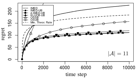
Figure 1: Regret approximated over $500$ runs for $\nu_{0}\!\in\!\mathcal{D}$.

Remark 15

It is generally observed in bandit problems that theoretical asymptotic lower bounds on the regret are larger than the actual regret in finite horizon, as is it in Figure 1.

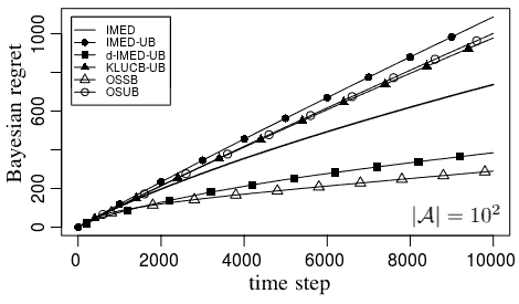
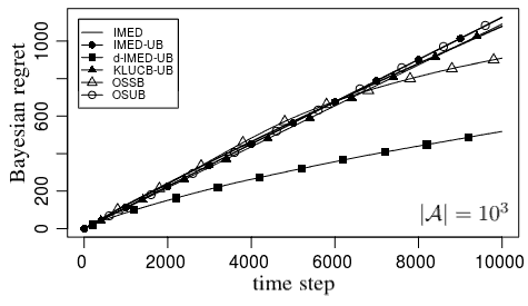
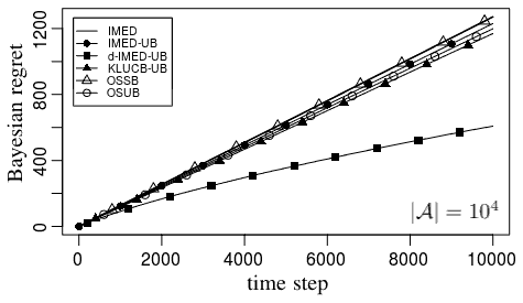
Figure 2: Regret averaged over $500$ random configurations in $\mathcal{D}$.

Conclusion

In this paper, we have revisited the setup of unimodal multi-armed bandits: We introduced three novel variants, two based on the IMED strategy and a second one using a KLUCB type index but modified using tools similar to IMED. These strategies do not require forcing to play specific arms (unlike for instance OSUB) on top of the naturally introduced score. Remarkably, the IMED-UB and d-IMED-UB strategies do not require any optimization procedure, which can be interesting for practitioners. We also provided a novel proof strategy (inspired from IMED), in which we make explicit empirical lower and upper bounds, before tackling the handling of bad events by more standard concentration tools. This proof technique greatly simplifies and shorten the analysis of IMED-UB (compared to that of OSUB), and is also employed to analyze KLUCB-UB and d-IMED-UB, in a somewhat unified way. Last, we provided numerical experiments that show the practical advantages of the novel approach over the OSUB strategy.

A IMED-UB finite time analysis

We regroup in this section, for completeness, the proofs of the remaining lemmas used in the analysis of IMED-UB in Section 4.

A.1 Concentration lemmas

We state two concentration lemmas that do not depend on the followed strategy. Lemma 16 comes from Lemma B.1 in Combes and Proutiere (2014) and Lemma 17 comes from Lemma 14 in Honda and Takemura (2015). Proofs are provided in Appendix B.

Lemma 16 (Concentration inequalities)

Independently of the considered strategy, for all set of Gaussian or Bernoulli distributions $\nu\!\in\!\mathcal{D}$, for all $0\!<\!\varepsilon\!\leqslant\!1/2$, for all $a,a^{\prime}\!\in\!\mathcal{A}$, we have

$$\mathbb{E}_{\nu}\!\left[\sum\limits_{t\geqslant 1}\mathbb{I}_{\left\{a_{t+1}=a,\ N_{a^{\prime}}(t)\geqslant N_{a}(t),\ \left|{{\widehat{\mu}}}_{a^{\prime}}(t)-\mu_{a^{\prime}}\right|\geqslant\varepsilon\right\}}\right]\leqslant\dfrac{10}{\varepsilon^{4}}\,.$$

Lemma 17 (Large deviation probabilities)

Let us consider a set of Gaussian or Bernoulli distributions $\nu\!\in\!\mathcal{D}$. Let $0\!<\!\varepsilon\!\leqslant\!\min(1\!-\!\mu^{\star},1/2)$ and $a\!\in\!\mathcal{A}$. Let $\lambda\!=\!\mu_{a}\!-\!\varepsilon$. Then, independently of the considered strategy, we have

$$\mathbb{E}_{\nu}\!\left[\sum\limits_{n\geqslant 1}\mathbb{I}_{\left\{{{\widehat{\mu}}}_{a}^{n}<\lambda\right\}}n\exp\!\left(n\text{KL}\!\left({{\widehat{\mu}}}_{a}^{n}\right.\!\!\left|\lambda\right)\right)\right]\leqslant\dfrac{23\log(1/\varepsilon)}{\varepsilon^{6}}\,.$$

A.2 Proof of Lemma 13 (Bounded subsets of times)

Using Lemma 10 we have

$$\forall t\geqslant 1,\quad N_{a_{t+1}}(t)\leqslant N_{\widehat{a}^{\star}_{t}}(t)\,.$$

Since $\widehat{a}^{\star}_{t}\!\in\!\mathop{\mathrm{argmin}}\limits_{\widehat{a}^{\star}\in\widehat{\mathcal{A}}^{\star}(t)}N_{\widehat{a}^{\star}}(t)$, this implies

$$\forall t\geqslant 1,\forall\widehat{a}^{\star}\in\widehat{\mathcal{A}}^{\star}(t),\quad N_{a_{t+1}}(t)\leqslant N_{\widehat{a}^{\star}_{t}}(t)\leqslant N_{\widehat{a}^{\star}}(t)\,.$$

Then, based on the concentration inequalities from Lemma 16, we obtain

$$\mathbb{E}_{\nu}[\left|\mathcal{E}_{\varepsilon}^{c}\right|] \leqslant \sum\limits_{a,a^{\prime}\in\mathcal{A}}\mathbb{E}_{\nu}\!\left[\sum\limits_{t\geqslant 1}{\mathbb{I}_{\left\{a_{t+1}=a,\ N_{a^{\prime}}(t)\geqslant N_{a}(t),\ \left|{{\widehat{\mu}}}_{a^{\prime}}(t)-\mu_{a^{\prime}}\right|\geqslant\varepsilon\right\}}}\right]$$

$$\leqslant \sum\limits_{a,a^{\prime}\in\mathcal{A}}\dfrac{10}{\varepsilon^{4}}$$

$$\leqslant \dfrac{10\left|\mathcal{A}\right|^{2}}{\varepsilon^{4}}\,.$$

Furthermore, for $t\!\geqslant\!1$ and $a\!\in\!\mathcal{A}$, we have

$$\log\!\left(N_{a_{t+1}}(t)\right)\leqslant N_{a}(t)\text{KL}\!\left({{\widehat{\mu}}}_{a}(t)\right.\!\!\left|\lambda_{a}\right)+\log\!\left(N_{a}(t)\right)\quad\Leftrightarrow\quad N_{a_{t+1}}(t)\leqslant N_{a}(t)\exp\!\left(N_{a}(t)\text{KL}\!\left({{\widehat{\mu}}}_{a}(t)\right.\!\!\left|\lambda_{a}\right)\right)\,,$$

where $\lambda_{a}\!=\!\mu_{a}\!-\!\varepsilon$ for all arm $a\!\in\!\mathcal{A}$.  
Thus, we have

$$\left|\Lambda_{\varepsilon}\right| \leqslant \sum\limits_{t\geqslant 1}\sum\limits_{a\in\mathcal{V}_{\widehat{a}^{\star}_{t}}\!\setminus\!\left\{a_{t+1},\widehat{a}^{\star}_{t}\right\}}\mathbb{I}_{\left\{{{\widehat{\mu}}}_{a}(t)<\lambda_{a}\textnormal{ and }N_{a_{t+1}}(t)\leqslant N_{a}(t)\exp\left(N_{a}(t)\text{KL}({{\widehat{\mu}}}_{a}(t)|\lambda_{a})\right)\right\}}$$

$$= \sum\limits_{t\geqslant 1}\sum\limits_{\widehat{a}^{\star}\in\mathcal{A}}\sum\limits_{a^{\prime}\in\left\{\widehat{a}^{\star}\right\}\cup\mathcal{V}_{\widehat{a}^{\star}}}\sum\limits_{a\in\mathcal{V}_{\widehat{a}^{\star}}\!\setminus\!\left\{a^{\prime},\widehat{a}^{\star}\right\}}\sum\limits_{n\geqslant 1}\mathbb{I}_{\left\{\widehat{a}^{\star}_{t}=\widehat{a}^{\star},a_{t+1}=a^{\prime},N_{a}(t)=n\right\}}\mathbb{I}_{\left\{{{\widehat{\mu}}}_{a}^{n}<\lambda_{a},\ N_{a^{\prime}}(t)\leqslant n\exp\left(n\text{KL}({{\widehat{\mu}}}_{a}^{n}|\lambda_{a})\right)\right\}}$$

$$\leqslant \sum\limits_{t\geqslant 1}\sum\limits_{\widehat{a}^{\star}\in\mathcal{A}}\sum\limits_{a^{\prime}\in\left\{\widehat{a}^{\star}\right\}\cup\mathcal{V}_{\widehat{a}^{\star}}}\sum\limits_{a\in\mathcal{V}_{\widehat{a}^{\star}}\!\setminus\!\left\{a^{\prime},\widehat{a}^{\star}\right\}}\sum\limits_{n\geqslant 1}\mathbb{I}_{\left\{a_{t+1}=a^{\prime}\right\}}\mathbb{I}_{\left\{{{\widehat{\mu}}}_{a}^{n}<\lambda_{a}\right\}}\mathbb{I}_{\left\{N_{a^{\prime}}(t)\leqslant n\exp\left(n\text{KL}({{\widehat{\mu}}}_{a}^{n}|\lambda_{a})\right)\right\}}$$

$$= \sum\limits_{\widehat{a}^{\star}\in\mathcal{A}}\sum\limits_{a^{\prime}\in\left\{\widehat{a}^{\star}\right\}\cup\mathcal{V}_{\widehat{a}^{\star}}}\sum\limits_{a\in\mathcal{V}_{\widehat{a}^{\star}}\!\setminus\!\left\{a^{\prime},\widehat{a}^{\star}\right\}}\sum\limits_{n\geqslant 1}\mathbb{I}_{\left\{{{\widehat{\mu}}}_{a}^{n}<\lambda_{a}\right\}}\sum\limits_{t\geqslant 1}\mathbb{I}_{\left\{a_{t+1}=a^{\prime}\textnormal{ and }N_{a^{\prime}}(t)\leqslant n\exp\left(n\text{KL}({{\widehat{\mu}}}_{a}^{n}|\lambda_{a})\right)\right\}}$$

$$\leqslant \sum\limits_{\widehat{a}^{\star}\in\mathcal{A}}\sum\limits_{a^{\prime}\in\left\{\widehat{a}^{\star}\right\}\cup\mathcal{V}_{\widehat{a}^{\star}}}\sum\limits_{a\in\mathcal{V}_{\widehat{a}^{\star}}\!\setminus\!\left\{a^{\prime},\widehat{a}^{\star}\right\}}\sum\limits_{n\geqslant 1}\mathbb{I}_{\left\{{{\widehat{\mu}}}_{a}^{n}<\lambda_{a}\right\}}n\exp\!\left(n\text{KL}\!\left({{\widehat{\mu}}}_{a}^{n}\right.\!\!\left|\lambda_{a}\right)\right)$$

$$\leqslant \sum\limits_{\widehat{a}^{\star}\in\mathcal{A}}\sum\limits_{a^{\prime}\in\left\{\widehat{a}^{\star}\right\}\cup\mathcal{V}_{\widehat{a}^{\star}}}\sum\limits_{a\in\mathcal{V}_{\widehat{a}^{\star}}\!\setminus\!\left\{a^{\prime},\widehat{a}^{\star}\right\}}\sum\limits_{n\geqslant 1}\mathbb{I}_{\left\{{{\widehat{\mu}}}_{a}^{n}<\lambda_{a}\right\}}n\exp\!\left(n\text{KL}\!\left({{\widehat{\mu}}}_{a}^{n}\right.\!\!\left|\lambda_{a}\right)\right)$$

and

$$\mathbb{E}_{\nu}[\left|\Lambda_{\varepsilon}\right|]\leqslant\sum\limits_{\widehat{a}^{\star}\in\mathcal{A}}\sum\limits_{a^{\prime}\in\left\{\widehat{a}^{\star}\right\}\cup\mathcal{V}_{\widehat{a}^{\star}}}\sum\limits_{a\in\mathcal{V}_{\widehat{a}^{\star}}\!\setminus\!\left\{a^{\prime},\widehat{a}^{\star}\right\}}\mathbb{E}_{\nu}\!\left[\sum\limits_{n\geqslant 1}\mathbb{I}_{\left\{{{\widehat{\mu}}}_{a}^{n}<\lambda_{a}\right\}}n\exp\!\left(n\text{KL}\!\left({{\widehat{\mu}}}_{a}^{n}\right.\!\!\left|\lambda_{a}\right)\right)\right]\,.$$

Then, by applying Lemma 17 based on large deviation probabilities, we have

$$\forall a\in\mathcal{A},\quad\mathbb{E}_{\nu}\!\left[\sum\limits_{n\geqslant 1}\mathbb{I}_{\left\{{{\widehat{\mu}}}_{a}^{n}<\lambda_{a}\right\}}n\exp\left(n\text{KL}({{\widehat{\mu}}}_{a}^{n}|\lambda_{a})\right)\right]\leqslant\dfrac{23\log(1/\varepsilon)}{\varepsilon^{6}}\,.$$

It comes:

$$\mathbb{E}_{\nu}[\left|\Lambda_{\varepsilon}\right|]\leqslant\sum\limits_{\widehat{a}^{\star}\in\mathcal{A}}\sum\limits_{a^{\prime}\in\left\{\widehat{a}^{\star}\right\}\cup\mathcal{V}_{\widehat{a}^{\star}}}\sum\limits_{a\in\mathcal{V}_{\widehat{a}^{\star}}\!\setminus\!\left\{a^{\prime},\widehat{a}^{\star}\right\}}\dfrac{23\log(1/\varepsilon)}{\varepsilon^{6}}\leqslant 23d^{2}\left|\mathcal{A}\right|\dfrac{\log(1/\varepsilon)}{\varepsilon^{6}}\,.$$

B Concentration lemmas

Lemma Independently of the considered strategy, for all set of Gaussian or Bernoulli distributions $\nu\!\in\!\mathcal{D}$, for all $0\!<\!\varepsilon\!\leqslant\!1/2$, for all $a,a^{\prime}\!\in\!\mathcal{A}$, we have

$$\mathbb{E}_{\nu}\left[\sum\limits_{t\geqslant 1}\mathbb{I}_{\left\{a_{t+1}=a,\ N_{a^{\prime}}(t)\geqslant N_{a}(t),\ \left|{{\widehat{\mu}}}_{a^{\prime}}(t)-\mu_{a^{\prime}}\right|\geqslant\varepsilon\right\}}\right]\leqslant\dfrac{10}{\varepsilon^{4}}\,.$$

Proof  Considering the stopping times $\tau_{a,n}\!=\!\inf{\left\{t\!\geqslant\!1,N_{a}(t)\!=\!n\right\}}$ we will rewrite the sum  
$\sum\limits_{t\geqslant 1}\mathbb{I}_{\left\{a_{t+1}=a,\ N_{a^{\prime}}(t)\geqslant N_{a}(t),\ \left|{{\widehat{\mu}}}_{a^{\prime}}(t)-\mu_{a^{\prime}}\right|\geqslant\varepsilon\right\}}$ and use an Hoeffding’s type argument for distributions with support included in $[0,1]$.

$$\sum\limits_{t\geqslant 1}\mathbb{I}_{\left\{a_{t+1}=a,\ N_{a^{\prime}}(t)\geqslant N_{a}(t),\ \left|{{\widehat{\mu}}}_{a^{\prime}}(t)-\mu_{a^{\prime}}\right|\geqslant\varepsilon\right\}}$$

$$= \sum\limits_{t\geqslant 1}\sum\limits_{n\geqslant 2,m\geqslant 1}\mathbb{I}_{\left\{\tau_{a,n}=t+1,N_{a^{\prime}}(t)=m\right\}}\mathbb{I}_{\left\{m\geqslant n-1,\ \left|{{\widehat{\mu}}}_{a^{\prime}}^{m}-\mu_{a^{\prime}}\right|\geqslant\varepsilon\right\}}$$

$$= \sum\limits_{m\geqslant 1}\sum\limits_{n\geqslant 2}\mathbb{I}_{\left\{m\geqslant n-1,\ \left|{{\widehat{\mu}}}_{a^{\prime}}^{m}-\mu_{a^{\prime}}\right|\geqslant\varepsilon\right\}}\sum\limits_{t\geqslant 1}\mathbb{I}_{\left\{\tau_{a,n}=t+1,N_{a^{\prime}}(t)=m\right\}}$$

$$\leqslant \sum\limits_{m\geqslant 1}\sum\limits_{n\geqslant 2}\mathbb{I}_{\left\{m\geqslant n-1,\ \left|{{\widehat{\mu}}}_{a^{\prime}}^{m}-\mu_{a^{\prime}}\right|\geqslant\varepsilon\right\}}\sum\limits_{t\geqslant 1}\mathbb{I}_{\left\{\tau_{a,n}=t+1\right\}}$$

$$\leqslant \sum\limits_{m\geqslant 1}\sum\limits_{n\geqslant 2}\mathbb{I}_{\left\{m\geqslant n-1,\ \left|{{\widehat{\mu}}}_{a^{\prime}}^{m}-\mu_{a^{\prime}}\right|\geqslant\varepsilon\right\}}$$

Taking the expectation , it comes

$$\mathbb{E}_{\nu}\left[\sum\limits_{t\geqslant 1}\mathbb{I}_{\left\{a_{t+1}=a,\ N_{a^{\prime}}(t)\geqslant N_{a}(t),\ \left|{{\widehat{\mu}}}_{a^{\prime}}(t)-\mu_{a^{\prime}}\right|\geqslant\varepsilon\right\}}\right]$$

$$\leqslant \sum\limits_{m\geqslant 1}\sum\limits_{n\geqslant 2}\mathbb{I}_{\left\{m\geqslant n-1\right\}}\mathbb{P}_{\nu}\left(\left|{{\widehat{\mu}}}_{a^{\prime}}^{m}-\mu_{a^{\prime}}\right|\geqslant\varepsilon\right)$$

$$\leqslant \sum\limits_{m\geqslant 1}\sum\limits_{n\geqslant 2}\mathbb{I}_{\left\{m\geqslant n-1\right\}}\max\!\left(2e^{-2m\varepsilon^{2}},\ 2e^{-m\varepsilon^{2}/2}\right)\qquad\textnormal{(Hoeffding's inequality)}$$

$$= \sum\limits_{m\geqslant 1}\sum\limits_{n\geqslant 2}\mathbb{I}_{\left\{m\geqslant n-1\right\}}2e^{-m\varepsilon^{2}/2}$$

$$= 2\sum\limits_{m\geqslant 1}me^{-m\varepsilon^{2}/2}$$

$$= \dfrac{2e^{-\varepsilon^{2}/2}}{(1-e^{-\varepsilon^{2}/2})^{2}}=\dfrac{2e^{\varepsilon^{2}/2}}{(e^{\varepsilon^{2}/2}-1)^{2}}\leqslant\dfrac{8e^{1/8}}{\varepsilon^{4}}\leqslant\dfrac{10}{\varepsilon^{4}}\,.\qquad\textnormal{(}0<\varepsilon\leqslant 1/2\textnormal{)}$$

 

Lemma Let us consider a set of Gaussian or Bernoulli distributions $\nu\!\in\!\mathcal{D}$. Let $0\!<\!\varepsilon\!\leqslant\!\min(1\!-\!\mu^{\star},1/2)$ and $a\!\in\!\mathcal{A}$. Let $\lambda\!=\!\mu_{a}\!-\!\varepsilon$. Then, independently of the considered strategy, we have

$$\mathbb{E}_{\nu}\left[\sum\limits_{n\geqslant 1}\mathbb{I}_{\left\{{{\widehat{\mu}}}_{a}^{n}<\lambda\right\}}n\exp(n\text{KL}\!\left({{\widehat{\mu}}}_{a}^{n}\right.\!\!\left|\lambda\right))\right]\leqslant\dfrac{23\log(1/\varepsilon)}{\varepsilon^{6}}\,.$$

We provide two proofs, one for Gaussian distributions and another for Bernoulli distributions, that can be read separately.

Proof [For Gaussian distributions] The proof is based on a Chernoff type inequality and a calculation by measurement change.

Since $\nu_{a}\sim\mathcal{N}(\mu_{a},1)$ we have for all $\varepsilon>0$,

$$\forall n\geqslant 1,\quad\mathbb{P}_{\nu}({{\widehat{\mu}}}_{a}^{n}-\mu_{a}\leqslant-\varepsilon)\leqslant e^{-n\varepsilon^{2}/2}\,.$$

In addition, $\forall\mu,\mu^{\prime}\!\in\!\mathbb{R},\quad\text{KL}(\mu|\mu^{\prime})\!=\!\dfrac{(\mu\!-\!\mu^{\prime})^{2}}{2}$. Let $n\geqslant 1$. We have:

$$\mathbb{E}_{\nu}\left[\mathbb{I}_{\left\{{{\widehat{\mu}}}_{a}^{n}\leqslant\lambda\right\}}ne^{n\text{KL}({{\widehat{\mu}}}_{a}^{n}|\lambda)}\right]$$

$$= \int_{0}^{\infty}\mathbb{P}_{\nu}\left(\mathbb{I}_{\left\{{{\widehat{\mu}}}_{a}^{n}\leqslant\lambda\right\}}ne^{n\text{KL}({{\widehat{\mu}}}_{a}^{n}|\lambda)}>x\right)\mathrm{d}x$$

$$= \int_{0}^{\infty}\mathbb{P}_{\nu}\left(ne^{n\text{KL}({{\widehat{\mu}}}_{a}^{n}|\lambda)}>x,\ {{\widehat{\mu}}}_{a}^{n}\leqslant\lambda\right)\mathrm{d}x$$

$$= \int_{-\infty}^{\infty}n^{2}e^{nu}\mathbb{P}_{\nu}\left(\text{KL}({{\widehat{\mu}}}_{a}^{n}|\lambda)>u,\ {{\widehat{\mu}}}_{a}^{n}\leqslant\lambda\right)\mathrm{d}u\qquad(\textnormal{variable change }x=ne^{nu},\ \mathrm{d}x=n^{2}e^{nu}\mathrm{d}u)$$

$$= \int_{-\infty}^{0}n^{2}e^{nu}\mathbb{P}_{\nu}\left(\text{KL}({{\widehat{\mu}}}_{a}^{n}|\lambda)>u,\ {{\widehat{\mu}}}_{a}^{n}\leqslant\lambda\right)\mathrm{d}u+\int_{0}^{\infty}n^{2}e^{nu}\mathbb{P}_{\nu}\left(\text{KL}({{\widehat{\mu}}}_{a}^{n}|\lambda)>u,\ {{\widehat{\mu}}}_{a}^{n}\leqslant\lambda\right)\mathrm{d}u$$

$$= n^{2}\mathbb{P}_{\nu}\left({{\widehat{\mu}}}_{a}^{n}-\mu_{a}\leqslant-\varepsilon\right)\int_{-\infty}^{0}e^{nu}\mathrm{d}u+\int_{0}^{\infty}n^{2}e^{nu}\mathbb{P}_{\nu}\left({{\widehat{\mu}}}_{a}^{n}-\mu_{a}\leqslant-\varepsilon-\sqrt{2u}\right)\mathrm{d}u$$

$$\leqslant n^{2}e^{-n\varepsilon^{2}/2}\dfrac{1}{n}+\int_{0}^{\infty}n^{2}e^{nu}e^{-n(\varepsilon+\sqrt{2u})^{2}/2}\mathrm{d}u$$

$$= ne^{-n\varepsilon^{2}/2}+n^{2}e^{-n\varepsilon^{2}/2}\int_{0}^{\infty}e^{-n\varepsilon\sqrt{2u}}\mathrm{d}u$$

$$= ne^{-n\varepsilon^{2}/2}+n^{2}e^{-n\varepsilon^{2}/2}\int_{0}^{\infty}ye^{-n\varepsilon y}\mathrm{d}y\qquad(\textnormal{variable change }u=\dfrac{y^{2}}{2},\ \mathrm{d}u=y\mathrm{d}y)$$

$$= ne^{-n\varepsilon^{2}/2}+n^{2}e^{-n\varepsilon^{2}/2}\dfrac{1}{(n\varepsilon)^{2}}$$

$$= ne^{-n\varepsilon^{2}/2}+\dfrac{1}{\varepsilon^{2}}e^{-n\varepsilon^{2}/2}$$

To ends the proof, we use the following equalities for $r>0$

$$\sum\limits_{n\geqslant 1}e^{-nr}=\dfrac{e^{-r}}{1-e^{-r}}$$

$$\sum\limits_{n\geqslant 1}ne^{-nr}=\dfrac{e^{-r}}{(1-e^{-r})^{2}}$$

and obtain

$$\mathbb{E}_{\nu}\left[\sum\limits_{n\geqslant 1}\mathbb{I}_{\left\{{{\widehat{\mu}}}_{a}^{n}<\lambda\right\}}n\exp(n\text{KL}({{\widehat{\mu}}}_{a}^{n}|\lambda))\right]\leqslant\dfrac{1}{\varepsilon^{2}}\dfrac{e^{-\varepsilon^{2}/2}}{1-e^{-\varepsilon^{2}/2}}+\dfrac{e^{-\varepsilon^{2}/2}}{(1-e^{-\varepsilon^{2}/2})^{2}}\leqslant\dfrac{10}{\varepsilon^{4}}\,.$$

 

Proof [For Bernoulli distributions] The proof is based on a Chernoff type inequality and a calculation by measurement change.

Since the support of $\nu_{a}$ is included in $[0,1]$ we have by Chernoff’s and Pinsker’s inequalities

$$\forall 0\leqslant v\leqslant\mu_{a},\forall n\geqslant 1,\quad\mathbb{P}_{\nu}({{\widehat{\mu}}}_{a}^{n}\leqslant v)\leqslant e^{-n\text{kl}(v|\mu_{a})}\leqslant e^{-2n(\mu_{a}-v)^{2}}\,.$$

Let $n\geqslant 1$. We have

$$\mathbb{E}_{\nu}\left[\mathbb{I}_{\left\{{{\widehat{\mu}}}_{a}^{n}\leqslant\lambda\right\}}ne^{n\text{kl}({{\widehat{\mu}}}_{a}^{n}|\lambda)}\right]$$

$$= \int_{0}^{\infty}\mathbb{P}_{\nu}\left(\mathbb{I}_{\left\{{{\widehat{\mu}}}_{a}^{n}\leqslant\lambda\right\}}ne^{n\text{kl}({{\widehat{\mu}}}_{a}^{n}|\lambda)}>x\right)\mathrm{d}x$$

$$= \int_{0}^{\infty}\mathbb{P}_{\nu}\left(ne^{n\text{kl}({{\widehat{\mu}}}_{a}^{n}|\lambda)}>x,\ {{\widehat{\mu}}}_{a}^{n}\leqslant\lambda\right)\mathrm{d}x$$

$$= \int_{-\infty}^{\infty}n^{2}e^{nu}\mathbb{P}_{\nu}\left(\text{kl}\!\left({{\widehat{\mu}}}_{a}^{n}\right.\!\!\left|\lambda\right)>u,\ {{\widehat{\mu}}}_{a}^{n}\leqslant\lambda\right)\mathrm{d}u\qquad(\textnormal{variable change }x=ne^{nu},\ \mathrm{d}x=n^{2}e^{nu}\mathrm{d}u)$$

$$= \int_{-\infty}^{0}n^{2}e^{nu}\mathbb{P}_{\nu}\left(\text{kl}\!\left({{\widehat{\mu}}}_{a}^{n}\right.\!\!\left|\lambda\right)>u,\ {{\widehat{\mu}}}_{a}^{n}\leqslant\lambda\right)\mathrm{d}u+\int_{0}^{\text{kl}(0|\lambda)}n^{2}e^{nu}\mathbb{P}_{\nu}\left(\text{kl}\!\left({{\widehat{\mu}}}_{a}^{n}\right.\!\!\left|\lambda\right)>u,\ {{\widehat{\mu}}}_{a}^{n}\leqslant\lambda\right)\mathrm{d}u\,.$$

On the one hand

$$\int_{-\infty}^{0}n^{2}e^{nu}\mathbb{P}_{\nu}\left(\text{kl}\!\left({{\widehat{\mu}}}_{a}^{n}\right.\!\!\left|\lambda\right)>u,\ {{\widehat{\mu}}}_{a}^{n}\leqslant\lambda\right)\mathrm{d}u$$

$$= n^{2}\mathbb{P}_{\nu}\left({{\widehat{\mu}}}_{a}^{n}\leqslant\lambda\right)\int_{-\infty}^{0}e^{nu}\mathrm{d}u$$

$$\leqslant n^{2}e^{-2n(\mu_{a}-\lambda)^{2}}\dfrac{1}{n}$$

$$= ne^{-2n\varepsilon^{2}}\,.$$

On the other hand, using variable change $u\!=\!\text{kl}(v|\lambda)$ and Lemma 18, it comes

$$\int_{0}^{\text{kl}(0|\lambda)}n^{2}e^{nu}\mathbb{P}_{\nu}\left(\text{kl}\!\left({{\widehat{\mu}}}_{a}^{n}\right.\!\!\left|\lambda\right)>u,\ {{\widehat{\mu}}}_{a}^{n}\leqslant\lambda\right)\mathrm{d}u$$

$$= \int_{0}^{\lambda}n^{2}e^{n\text{kl}(v|\lambda)}\mathbb{P}_{\nu}\left(\text{kl}\!\left({{\widehat{\mu}}}_{a}^{n}\right.\!\!\left|\lambda\right)>\text{kl}\!\left(v\right.\!\!\left|\lambda\right),\ {{\widehat{\mu}}}_{a}^{n}\leqslant\lambda\right)\left[-\dfrac{\partial\text{kl}}{\partial p}(v|\lambda)\right]\mathrm{d}v$$

$$= \int_{0}^{\lambda}n^{2}e^{n\text{kl}(v|\lambda)}\mathbb{P}_{\nu}\left({{\widehat{\mu}}}_{a}^{n}<v\right)\left[-\dfrac{\partial\text{kl}}{\partial p}(v|\lambda)\right]\mathrm{d}v$$

$$\leqslant \int_{0}^{\lambda}n^{2}e^{n\text{kl}(v|\lambda)}e^{-n\text{kl}(v|\mu_{a})}\left[-\dfrac{\partial\text{kl}}{\partial p}(v|\lambda)\right]\mathrm{d}v$$

$$= \int_{0}^{\lambda}n^{2}e^{-n\left(\text{kl}(v|\mu_{a})-\text{kl}(v|\lambda)\right)}\left[-\dfrac{\partial\text{kl}}{\partial p}(v|\lambda)\right]\mathrm{d}v$$

$$\leqslant \int_{0}^{\lambda}n^{2}e^{-n\frac{(\mu_{a}-\lambda)^{2}}{2}}\left[-\dfrac{\partial\text{kl}}{\partial p}(v|\lambda)\right]\mathrm{d}v\qquad\textnormal{( Lemma~{}\ref{kl_inequality})}$$

$$= \text{kl}(0|\lambda)n^{2}e^{-n\varepsilon^{2}/2}$$

$$\leqslant \left(-\log(1-\mu^{\star})\right)n^{2}e^{-n\varepsilon^{2}/2}$$

$$\leqslant \log(1/\varepsilon)n^{2}e^{-n\varepsilon^{2}/2}\,,$$

where $\dfrac{\partial\text{kl}}{\partial p}$ corresponds to the derivative of the $\text{kl}(\cdot|\cdot)$ according to the first variable. Thus we have

$$\mathbb{E}_{\nu}\left[\mathbb{I}_{\left\{{{\widehat{\mu}}}_{a}^{n}\leqslant\lambda\right\}}ne^{n\text{kl}({{\widehat{\mu}}}_{a}^{n}|\lambda)}\right]\leqslant ne^{-2n\varepsilon^{2}}+\log(1/\varepsilon)n^{2}e^{-n\varepsilon^{2}/2}\,.$$

To ends the proof, we use the following equalities for $r>0$

$$\sum\limits_{n\geqslant 1}e^{-nr}=\dfrac{e^{-r}}{1-e^{-r}}=\dfrac{1}{e^{r}-1}$$

$$\sum\limits_{n\geqslant 1}ne^{-nr}=\dfrac{e^{r}}{(e^{r}-1)^{2}}=\dfrac{1}{e^{r}-1}+\dfrac{1}{(e^{r}-1)^{2}}$$

$$\sum\limits_{n\geqslant 1}n^{2}e^{-nr}=\dfrac{e^{r}}{(e^{r}-1)^{2}}+\dfrac{2e^{r}}{(e^{r}-1)^{3}}=\dfrac{e^{2r}+e^{r}}{(e^{r}-1)^{3}}$$

and obtain

$$\mathbb{E}_{\nu}\left[\sum\limits_{n\geqslant 1}\mathbb{I}_{\left\{{{\widehat{\mu}}}_{a}^{n}<\lambda\right\}}n\exp(n\text{kl}\!\left({{\widehat{\mu}}}_{a}^{n}\right.\!\!\left|\lambda\right))\right]\leqslant\dfrac{e^{2\varepsilon^{2}}}{(e^{2\varepsilon^{2}}-1)^{2}}+\dfrac{\log(1/\varepsilon)e^{\varepsilon^{2}}+e^{\varepsilon^{2}/2}}{(e^{\varepsilon^{2}/2}-1)^{3}}\leqslant\dfrac{23\log(1/\varepsilon)}{\varepsilon^{6}}\,.$$

 

Lemma 18

For all $0\!\leqslant\!v\!\leqslant\lambda\!<\!\mu\!<\!1$ we have

$$\text{kl}\!\left(v\right.\!\!\left|\mu\right)-\text{kl}\!\left(v\right.\!\!\left|\lambda\right)\geqslant\dfrac{(\mu-\lambda)^{2}}{2}\,.$$

Proof  Using monotony of the $\text{kl}(\cdot|\cdot)$ we get

$$\text{kl}\!\left(v\right.\!\!\left|\mu\right)-\text{kl}\!\left(v\right.\!\!\left|\lambda\right)\geqslant\text{kl}\!\left(v\right.\!\!\left|\mu\right)-\text{kl}\!\left(v\left|\frac{\mu+\lambda}{2}\right.\right)\,.$$

Using convexity of the $\text{kl}(\cdot|\cdot)$ we get

$$\dfrac{\text{kl}\!\left(v\right.\!\!\left|\mu\right)-\text{kl}\!\left(v\left|\frac{\mu+\lambda}{2}\right.\right)}{\mu-\frac{\mu+\lambda}{2}}\geqslant\dfrac{\partial\text{kl}}{\partial q}\!\left(v\left|\frac{\mu+\lambda}{2}\right.\right)\geqslant\dfrac{\partial\text{kl}}{\partial q}\!\left(\lambda\left|\frac{\mu+\lambda}{2}\right.\right)\,,$$

where $\dfrac{\partial\text{kl}}{\partial q}$ corresponds to the derivative of the $\text{kl}(\cdot|\cdot)$ according to the second variable. From Lemma B.4 in Combes and Proutiere (2014) we have

$$\left(\frac{\mu+\lambda}{2}-\lambda\right)\dfrac{\partial\text{kl}}{\partial q}\!\left(\lambda\left|\frac{\mu+\lambda}{2}\right.\right)\geqslant\text{kl}\!\left(\lambda\left|\frac{\mu+\lambda}{2}\right.\right)\,.$$

Then Pinsker’s inequality implies

$$\left(\frac{\mu+\lambda}{2}-\lambda\right)\dfrac{\partial\text{kl}}{\partial q}\!\left(\lambda\left|\frac{\mu+\lambda}{2}\right.\right)\geqslant 2\left(\frac{\mu+\lambda}{2}-\lambda\right)^{2}=\dfrac{(\mu-\lambda)^{2}}{2}\,,$$

which ends the proof.  

C KLUCB-UB finite time analysis

KLUCB-UB strategy implies similar lower bounds and empirical upper bounds on the numbers of pulls as IMED-UB strategy. An additional random process $(\gamma_{t})_{t\geqslant 1}\!\in\!\left\{0,1\right\}$ appears in the empirical lower bounds induced by KLUCB-UB strategy (Lemma 19). When $\gamma_{t}\!=\!1$, the empirical bounds are the same of the ones induced by IMED-UB strategy. And we show that the process $(\gamma_{t})_{t\geqslant 1}$ reaches zero only a finite number of times for which a use of the empirical bounds is needed. Then, similar reasoning as the one developed in Section 4 can be re-used and gives similar finite time analysis.

C.1 Notations

Please, refer to Section 4.1.

C.2 Strategy-based empirical bounds

In this subsection, we provide empirical bounds very similar to the ones induced by IMED-UB strategy. We first establish preliminary results on the indexes.

It is noticeable that for all time step $t\!\geqslant\!1$,

$$\forall\widehat{a}^{\star}\in\widehat{\mathcal{A}}^{\star}(t),\quad U_{\widehat{a}^{\star}}(t)={{\widehat{\mu}}}_{\widehat{a}^{\star}}(t)={{\widehat{\mu}}}^{\star}(t)\,.$$ (3)

In addition for $a\!\notin\!\widehat{\mathcal{A}}^{\star}(t)$,

$$\textnormal{if }N_{a}(t)\geqslant N_{\widehat{a}^{\star}_{t}}(t)\,,\quad U_{a}(t)={{\widehat{\mu}}}_{a}(t)\text{\ \ and \ }U_{a}(t)<U_{\widehat{a}^{\star}_{t}}(t)\,,$$ (4)

$$\textnormal{if }N_{a}(t)<N_{\widehat{a}^{\star}_{t}}(t)\,,\quad N_{a}(t)\text{KL}\!\left({{\widehat{\mu}}}_{a}(t)\right.\!\!\left|U_{a}(t)\right)+\log\!\left(N_{a}(t)\right)=\log\!\left(N_{\widehat{a}^{\star}_{t}}(t)\right)\,.$$ (5)

In particular we have

$$N_{a_{t+1}}(t)\leqslant N_{\widehat{a}^{\star}_{t}}(t)$$ (6)

  and $$N_{a_{t+1}}(t)\text{KL}\!\left({{\widehat{\mu}}}_{a_{t+1}}(t)\right.\!\!\left|U_{a_{t+1}}(t)\right)+\log\!\left(N_{a_{t+1}}(t)\right)=\log\!\left(N_{\widehat{a}^{\star}_{t}}(t)\right)\,.$$ (7)

Lemma 19 (Empirical lower bounds)

Under KLUCB-UB, at each step time $t\!\geqslant\!1$,

$$1. \forall a\in\mathcal{V}_{\widehat{a}^{\star}_{t}},\quad\gamma_{t}\log\!\left(N_{a_{t+1}}(t)\right)\leqslant N_{a}(t)\text{KL}\!\left({{\widehat{\mu}}}_{a}(t)\right.\!\!\left|{{\widehat{\mu}}}^{\star}(t)\right)+\log\!\left((N_{a}(t)\right)$$

$$2. N_{a_{t+1}}(t)\leqslant N_{\widehat{a}^{\star}_{t}}(t)\,,$$

where $\gamma_{t}\!=\!\mathbb{I}_{\left\{a_{t+1}\in\widehat{\mathcal{A}}^{\star}(t)\right\}}\!+\!\mathbb{I}_{\left\{a_{t+1}\notin\widehat{\mathcal{A}}^{\star}(t)\text{\ \ and \ }\log(N_{a_{t+1}}(t))\leqslant N_{a_{t+1}}(t)\text{KL}({{\widehat{\mu}}}_{a_{t+1}}(t)|{{\widehat{\mu}}}^{\star}(t))\right\}}\!\in\!\left\{0,1\right\}$.

Proof  Let $t\!\geqslant\!1$. We have already seen that $N_{a_{t+1}}(t)\!\leqslant\!N_{\widehat{a}^{\star}_{t}}(t)$ in (6). This corresponds to point 2. In the following, we prove point 1.

For $a\!\in\!\mathcal{V}_{\widehat{a}^{\star}_{t}}$ such that $a\!=\!a_{t+1}$ or $N_{a}(t)\!\geqslant\!N_{a_{t+1}}(t)$, point 1. is naturally satisfied.

Let $a\!\in\!\mathcal{V}_{\widehat{a}^{\star}_{t}}$ such that $a\!\neq\!a_{t+1}$ and $N_{a}(t)\!<\!N_{a_{t+1}}(t)$.

Case 1 : $a_{t+1}\!=\!\widehat{a}^{\star}_{t}$  
Then $N_{a}(t)\!<\!N_{\widehat{a}^{\star}_{t}}(t)\leqslant N_{a_{t+1}}(t)$ and from equations (5) and (6) it comes:

$$\log\!\left(N_{a_{t+1}}(t)\right)=\log\!\left(N_{\widehat{a}^{\star}_{t}}(t)\right)\qquad N_{a}(t)\text{KL}\!\left({{\widehat{\mu}}}_{a}(t)\right.\!\!\left|U_{a}(t)\right)+\log\!\left(N_{a}(t)\right)=\log\!\left(N_{a_{t+1}}(t)\right)\,.$$

According to the followed strategy and equation 3

$${{\widehat{\mu}}}_{a}(t)\leqslant U_{a}(t)\leqslant U_{a_{t+1}}(t)\text{\ \ and \ }U_{a_{t+1}}(t)={{\widehat{\mu}}}^{\star}(t)\,.$$

Since $a_{t+1}=\widehat{a}^{\star}_{t}$, this implies

$${{\widehat{\mu}}}_{a}(t)\leqslant U_{a}(t)\leqslant{{\widehat{\mu}}}^{\star}(t)\,.$$

Then the monotony of the KL implies

$$\text{KL}\!\left({{\widehat{\mu}}}_{a}(t)\right.\!\!\left|U_{a}(t)\right)\leqslant\text{KL}\!\left({{\widehat{\mu}}}_{a}(t)\right.\!\!\left|{{\widehat{\mu}}}^{\star}(t)\right)$$

and

$$\log\!\left(N_{a_{t+1}}(t)\right) = N_{a}(t)\text{KL}\!\left({{\widehat{\mu}}}_{a}(t)\right.\!\!\left|U_{a}(t)\right)+\log\!\left(N_{a}(t)\right)$$

$$\leqslant N_{a}(t)\text{KL}\!\left({{\widehat{\mu}}}_{a}(t)\right.\!\!\left|{{\widehat{\mu}}}^{\star}(t)\right)+\log\!\left(N_{a}(t)\right)\,.$$

Case 2 : $a_{t+1}\!\neq\!\widehat{a}^{\star}(t)$  
From equations (5) and (7), we get

$$N_{a_{t+1}}(t)\text{KL}\!\left({{\widehat{\mu}}}_{a_{t+1}}(t)\right.\!\!\left|U_{a_{t+1}}(t)\right)+\log\!\left(N_{a_{t+1}}(t)\right)=N_{a}(t)\text{KL}\!\left({{\widehat{\mu}}}_{a}(t)\right.\!\!\left|U_{a}(t)\right)+\log\!\left(N_{a}(t)\right)\,.$$ (8)

Since $N_{a}(t)\!<\!N_{a_{t+1}}(t)$, this implies

$$\text{KL}\!\left({{\widehat{\mu}}}_{a_{t+1}}(t)\right.\!\!\left|U_{a_{t+1}}(t)\right)<\text{KL}\!\left({{\widehat{\mu}}}_{a}(t)\right.\!\!\left|U_{a}(t)\right)\,.$$

According to the followed strategy we have ${{\widehat{\mu}}}_{a}(t)\!\leqslant\!U_{a}(t)\!\leqslant\!U_{a_{t+1}}(t)$. Then, the monotony of the KL implies

$$\text{KL}\!\left({{\widehat{\mu}}}_{a}(t)\right.\!\!\left|U_{a}(t)\right)\leqslant\text{KL}\!\left({{\widehat{\mu}}}_{a}(t)\right.\!\!\left|U_{a_{t+1}}(t)\right)\,.$$

Thus, we have:

$$\text{KL}\!\left({{\widehat{\mu}}}_{a_{t+1}}(t)\right.\!\!\left|U_{a_{t+1}}(t)\right)<\text{KL}\!\left({{\widehat{\mu}}}_{a}(t)\right.\!\!\left|U_{a_{t+1}}(t)\right)\text{\ \ and \ }{{\widehat{\mu}}}_{a}(t)\leqslant U_{a_{t+1}}(t)\,.$$

Since ${{\widehat{\mu}}}_{a_{t+1}}(t)\!\leqslant\!U_{a_{t+1}}(t)$, the monotony of the KL implies

$${{\widehat{\mu}}}_{a}(t)<{{\widehat{\mu}}}_{a_{t+1}}(t)\,.$$

Then from equation (8) we deduce

$$N_{a_{t+1}}(t)\text{KL}\!\left({{\widehat{\mu}}}_{a_{t+1}}(t)\right.\!\!\left|U_{a_{t+1}}(t)\right)\leqslant N_{a}(t)\text{KL}\!\left({{\widehat{\mu}}}_{a}(t)\right.\!\!\left|U_{a_{t+1}}(t)\right)+\log\!\left(N_{a}(t)\right)$$

and

$$N_{a_{t+1}}(t)\leqslant\dfrac{\text{KL}\!\left({{\widehat{\mu}}}_{a}(t)\right.\!\!\left|U_{a_{t+1}}(t)\right)}{\text{KL}\!\left({{\widehat{\mu}}}_{a_{t+1}}(t)\right.\!\!\left|U_{a_{t+1}}(t)\right)}N_{a}(t)+\dfrac{\log\!\left(N_{a}(t)\right)}{\text{KL}\!\left({{\widehat{\mu}}}_{a_{t+1}}(t)\right.\!\!\left|U_{a_{t+1}}(t)\right)}\,.$$

Similarly, since ${{\widehat{\mu}}}_{a_{t+1}}(t)\!\leqslant\!{{\widehat{\mu}}}^{\star}(t)\!=\!U_{\widehat{a}^{\star}_{t}}(t)\!\leqslant\!U_{a_{t+1}}(t)$, the monotony of the KL implies

$$\text{KL}\!\left({{\widehat{\mu}}}_{a_{t+1}}(t)\right.\!\!\left|U_{a_{t+1}}(t)\right)\geqslant\text{KL}\!\left({{\widehat{\mu}}}_{a_{t+1}}(t)\right.\!\!\left|{{\widehat{\mu}}}^{\star}(t)\right)\,.$$

This implies

$$N_{a_{t+1}}(t)\leqslant\dfrac{\text{KL}\!\left({{\widehat{\mu}}}_{a}(t)\right.\!\!\left|U_{a_{t+1}}(t)\right)}{\text{KL}\!\left({{\widehat{\mu}}}_{a_{t+1}}(t)\right.\!\!\left|U_{a_{t+1}}(t)\right)}N_{a}(t)+\dfrac{\log\!\left(N_{a}(t)\right)}{\text{KL}\!\left({{\widehat{\mu}}}_{a_{t+1}}(t)\right.\!\!\left|{{\widehat{\mu}}}^{\star}(t)\right)}\,.$$

Since ${{\widehat{\mu}}}_{a}(t)\!\leqslant\!{{\widehat{\mu}}}_{a_{t+1}}(t)\!\leqslant\!{{\widehat{\mu}}}^{\star}(t)\!\leqslant\!U_{a_{t+1}}(t)$, we have from Lemma 21:

$$\dfrac{\text{KL}\!\left({{\widehat{\mu}}}_{a}(t)\right.\!\!\left|U_{a_{t+1}}(t)\right)}{\text{KL}\!\left({{\widehat{\mu}}}_{a_{t+1}}(t)\right.\!\!\left|U_{a_{t+1}}(t)\right)}\leqslant\dfrac{\text{KL}\!\left({{\widehat{\mu}}}_{a}(t)\right.\!\!\left|{{\widehat{\mu}}}^{\star}(t)\right)}{\text{KL}\!\left({{\widehat{\mu}}}_{a_{t+1}}(t)\right.\!\!\left|{{\widehat{\mu}}}^{\star}(t)\right)}\,.$$

This implies

$$N_{a_{t+1}}(t)\text{KL}\!\left({{\widehat{\mu}}}_{a_{t+1}}(t)\right.\!\!\left|{{\widehat{\mu}}}^{\star}(t)\right)\leqslant N_{a}(t)\text{KL}\!\left({{\widehat{\mu}}}_{a}(t)\right.\!\!\left|{{\widehat{\mu}}}^{\star}(t)\right)+\log\!\left(N_{a}(t)\right)\,.$$

 

Lemma 20 (Empirical upper bounds)

Under KLUCB-UB at each step time $t\!\geqslant\!1$,

$$N_{a_{t+1}}(t)\text{KL}\!\left({{\widehat{\mu}}}_{a_{t+1}}(t)\right.\!\!\left|{{\widehat{\mu}}}^{\star}(t)\right)\leqslant\log(t)\,.$$

Proof  From equation (7) we deduce

$$N_{a_{t+1}}(t)\text{KL}\!\left({{\widehat{\mu}}}_{a_{t+1}}(t)\right.\!\!\left|U_{a_{t+1}}(t)\right) \leqslant N_{a_{t+1}}(t)\text{KL}\!\left({{\widehat{\mu}}}_{a_{t+1}}(t)\right.\!\!\left|U_{a_{t+1}}(t)\right)+\log\!\left(N_{a_{t+1}}(t)\right)$$

$$= \log\!\left(N_{\widehat{a}^{\star}_{t}}(t)\right)$$

$$\leqslant \log(t)\,.$$

Furthermore, according to the followed strategy, we have

$${{\widehat{\mu}}}_{a_{t+1}}(t)\leqslant{{\widehat{\mu}}}^{\star}(t)=U_{\widehat{a}^{\star}_{t}}(t)\leqslant U_{a_{t+1}}(t)\,.$$

Then the monotony of the KL implies

$$\text{KL}\!\left({{\widehat{\mu}}}_{a_{t+1}}(t)\right.\!\!\left|{{\widehat{\mu}}}^{\star}(t)\right)\leqslant\text{KL}\!\left({{\widehat{\mu}}}_{a_{t+1}}(t)\right.\!\!\left|U_{a_{t+1}}(t)\right)$$

and

$$N_{a_{t+1}}(t)\text{KL}\!\left({{\widehat{\mu}}}_{a_{t+1}}(t)\right.\!\!\left|{{\widehat{\mu}}}^{\star}(t)\right)\leqslant N_{a_{t+1}}(t)\text{KL}\!\left({{\widehat{\mu}}}_{a_{t+1}}(t)\right.\!\!\left|U_{a_{t+1}}(t)\right)\leqslant\log\!\left(N_{\widehat{a}^{\star}_{t}}(t)\right)\leqslant\log(t)\,.$$

 

Lemma 21

Let $0\!\leqslant\!\mu\!\leqslant\!\mu^{\prime}\!\leqslant\!\mu^{\prime\prime}\!\leqslant\!1$. We have:

$$\forall u\in[\mu^{\prime\prime},1],\quad\dfrac{\text{KL}\!\left(\mu\right.\!\!\left|u\right)}{\text{KL}\!\left(\mu^{\prime}\right.\!\!\left|u\right)}\leqslant\dfrac{\text{KL}\!\left(\mu\right.\!\!\left|\mu^{\prime\prime}\right)}{\text{KL}\!\left(\mu^{\prime}\right.\!\!\left|\mu^{\prime\prime}\right)}\,.$$

We prove this lemma only for Bernoulli distributions when $\text{KL}(\cdot|\cdot)\!=\!\text{kl}(\cdot|\cdot)$. The proof is simpler for Gaussian distributions.

Proof [For Bernoulli distributions] We denote by $\frac{\partial\text{kl}}{\partial p}(\cdot|\cdot)$ and $\frac{\partial\text{kl}}{\partial q}(\cdot|\cdot)$ the derivatives of $\text{kl}(\cdot|\cdot)$ respectively according to the first and second variables. Let us consider $0\!\leqslant\!\mu\!\leqslant\!\mu^{\prime}\!\leqslant\!\mu^{\prime\prime}\!<\!1$ and $f\!:u\!\in\!(\mu^{\prime\prime},1)\!\mapsto\!\text{kl}\!\left(\mu^{\prime}\right.\!\!\left|\mu^{\prime\prime}\right)\text{kl}\!\left(\mu\right.\!\!\left|u\right)\!-\!\text{kl}\!\left(\mu\right.\!\!\left|\mu^{\prime\prime}\right)\text{kl}\!\left(\mu^{\prime}\right.\!\!\left|u\right)$. $f$ is a C-1 function and for $u\!\in\!(\mu^{\prime\prime},1)$,

$$f^{\prime}(u)=\text{kl}\!\left(\mu^{\prime}\right.\!\!\left|\mu^{\prime\prime}\right)\frac{\partial\text{kl}}{\partial q}(\mu|u)-\text{kl}\!\left(\mu\right.\!\!\left|\mu^{\prime\prime}\right)\frac{\partial\text{kl}}{\partial q}(\mu^{\prime}|u)=\dfrac{\text{kl}\!\left(\mu^{\prime}\right.\!\!\left|\mu^{\prime\prime}\right)(u-\mu)-\text{kl}\!\left(\mu\right.\!\!\left|\mu^{\prime\prime}\right)(u-\mu^{\prime})}{u(1-u)}\,.$$

Let us introduce $g\!:u\!\in\!(\mu^{\prime\prime},1)\!\mapsto\!\text{kl}\!\left(\mu^{\prime}\right.\!\!\left|\mu^{\prime\prime}\right)(u\!-\!\mu)\!-\!\text{kl}\!\left(\mu\right.\!\!\left|\mu^{\prime\prime}\right)(u\!-\!\mu^{\prime})$. $g$ is a C-1 function and for $u\!\in\!(\mu^{\prime\prime},1)$,

$$g^{\prime}(u)=\text{kl}\!\left(\mu^{\prime}\right.\!\!\left|\mu^{\prime\prime}\right)-\text{kl}\!\left(\mu\right.\!\!\left|\mu^{\prime\prime}\right)\,.$$

Since $\mu\!\leqslant\!\mu^{\prime}\!\leqslant\!\mu^{\prime\prime}$, the monotony of the kl implies $g^{\prime}(u)\!\leqslant\!0$. Then $g$ is a non-increasing function. In addition

$$g(\mu^{\prime\prime})=\text{kl}\!\left(\mu^{\prime}\right.\!\!\left|\mu^{\prime\prime}\right)(\mu^{\prime\prime}-\mu)-\text{kl}\!\left(\mu\right.\!\!\left|\mu^{\prime\prime}\right)(\mu^{\prime\prime}-\mu^{\prime})=(\mu^{\prime\prime}-\mu)\times\left(\text{kl}\!\left(\mu^{\prime}\right.\!\!\left|\mu^{\prime\prime}\right)-\dfrac{\text{kl}\!\left(\mu\right.\!\!\left|\mu^{\prime\prime}\right)}{(\mu^{\prime\prime}-\mu)}(\mu^{\prime\prime}-\mu^{\prime})\right)\,.$$

Lastly, let us consider $h\!:p\!\in\![0,\mu^{\prime\prime})\!\mapsto\!\frac{\text{kl}(p|\mu^{\prime\prime})}{\mu^{\prime\prime}-p}$. $h$ is a C-1 function or $p\!\in\![0,\mu^{\prime\prime})$,

$$h^{\prime}(p)=\dfrac{(\mu^{\prime\prime}-p)\frac{\partial\text{kl}}{\partial p}(p|\mu^{\prime\prime})+\text{kl}(p|\mu^{\prime\prime})}{(\mu^{\prime\prime}-p)^{2}}=\dfrac{-\text{kl}(\mu^{\prime\prime}|p)}{(\mu^{\prime\prime}-p)^{2}}\leqslant 0\,.$$

Then $h$ is a non-increasing function. In particular, since $\mu\!\leqslant\!\mu^{\prime}$,

$$\dfrac{\text{kl}\!\left(\mu\right.\!\!\left|\mu^{\prime\prime}\right)}{(\mu^{\prime\prime}-\mu)}\geqslant\dfrac{\text{kl}\!\left(\mu^{\prime}\right.\!\!\left|\mu^{\prime\prime}\right)}{(\mu^{\prime\prime}-\mu^{\prime})}\,.$$

This implies $g(\mu^{\prime\prime})\!\leqslant\!0$ and $g\!\leqslant\!0$, since $g$ is a non-increasing function. Then $f^{\prime}\!\leqslant\!0$ and $f$ is a non-increasing function. Since $f(\mu^{\prime\prime})\!=\!0$, this implies $f\!\leqslant\!0$, which ends the proof.  

C.3 Reliable current best arm and means

As in IMED-UB analysis, we consider the subset $\mathcal{T}_{\varepsilon}$ of times where everything is well behaved, that is: the current best arm corresponds to the true one and the empirical means of the best arm and the current chosen arm are $\varepsilon$-accurate for $0<\varepsilon<\varepsilon_{\nu}$, i.e.

$$\mathcal{T}_{\varepsilon}\coloneqq\left\{t\geqslant 1:\ \widehat{\mathcal{A}}^{\star}(t)=\left\{a^{\star}\right\}\text{\ \ and \ }\forall a\in\left\{a^{\star},a_{t+1}\right\},\ \left|{{\widehat{\mu}}}_{a}(t)-\mu_{a}\right|<\varepsilon\right\}\,.$$

We will show that its complementary set is finite on average. In order to prove this we decompose the set $\mathcal{T}_{\varepsilon}$ in the following way. Let $\mathcal{E}_{\varepsilon}$ be the set of times where the means are well estimated,

$$\mathcal{E}_{\varepsilon}\coloneqq\left\{t\geqslant 1:\ \forall a\in\widehat{\mathcal{A}}^{\star}(t)\cup\left\{a_{t+1}\right\},\ \left|{{\widehat{\mu}}}_{a}(t)-\mu_{a}\right|<\varepsilon\right\}\,,$$

and $\Lambda_{\varepsilon}$ the set of times where an arm that is not the current optimal neither pulled is underestimated

$$\Lambda_{\varepsilon}\!\coloneqq\!\left\{\!t\geqslant 1:\,\exists a\in\mathcal{V}_{\widehat{a}^{\star}_{t}}\!\setminus\!\left\{a_{t+1},\widehat{a}^{\star}_{t}\right\}\textnormal{\,s.t.\,}\left\{\begin{array}[]{l}\!{{\widehat{\mu}}}_{a}(t)<\mu_{a}-\varepsilon\\ \!\log\!\left(N_{a_{t+1}}(t)\right)\leqslant N_{a}(t)\text{KL}\!\left({{\widehat{\mu}}}_{a}(t)\right.\!\!\left|\mu_{a}-\varepsilon\right)+\log\!\left((N_{a}(t)\right)\end{array}\right.\!\!\right\}\,.$$

Then, in the same way as for Lemma 12, we can prove the following inclusion.

Lemma 22 (Relations between the subsets of times)

For $0<\varepsilon<\varepsilon_{\nu}$,

$$\mathcal{T}_{\varepsilon}^{c}\cap\left\{t\geqslant 1:\ \gamma_{t}=1\right\}\cap\mathcal{E}_{\varepsilon}\subset\Lambda_{\varepsilon}\,.$$ (9)

We can now resort to classical concentration arguments in order to control the size of these sets, which yields the following upper bounds.

Lemma 23 (Bounded subsets of times)

For $0<\varepsilon<\varepsilon_{\nu}$,

$$\mathbb{E}_{\nu}[\left|\mathcal{E}_{\varepsilon}^{c}\right|]\leqslant\dfrac{10(d+1)\left|\mathcal{A}\right|}{\varepsilon^{4}}\qquad\mathbb{E}_{\nu}[\left|\Lambda_{\varepsilon}\right|]\leqslant 23d^{2}\left|\mathcal{A}\right|\dfrac{\log(1/\varepsilon)}{\varepsilon^{6}}\qquad\mathbb{E}_{\nu}[\left|\left\{t\geqslant 1:\ \gamma_{t}=0\right\}\cap\mathcal{E}_{\varepsilon}\right|]\leqslant\dfrac{\left|\mathcal{A}\right|}{\varepsilon^{4}}\,,$$

where $d$ is the maximum degree of nodes in $G$.

Proof  Refer to Lemma 13 to prove $\mathbb{E}_{\nu}[\left|\mathcal{E}_{\varepsilon}^{c}\right|]\!\leqslant\!\frac{10(d+1)\left|\mathcal{A}\right|}{\varepsilon^{4}},\,\mathbb{E}_{\nu}[\left|\Lambda_{\varepsilon}\right|]\!\leqslant\!23d^{2}\left|\mathcal{A}\right|\frac{\log(1/\varepsilon)}{\varepsilon^{6}}$. It is exactly the same proof.

Let $t\!\in\!\left\{t\geqslant 1:\ \gamma_{t}=0\right\}\cap\mathcal{E}_{\varepsilon}$. Then $\gamma_{t}\!=\!0$. This implies

$$a_{t+1}\neq\widehat{a}^{\star}_{t}\text{\ \ and \ }\log\!\left(N_{a_{t+1}}(t)\right)>N_{a_{t+1}}(t)\text{KL}\!\left({{\widehat{\mu}}}_{a_{t+1}}(t)\right.\!\!\left|{{\widehat{\mu}}}^{\star}(t)\right)\,.$$

Since $t\!\in\!\mathcal{E}_{\varepsilon}$ and $\varepsilon\!<\!\varepsilon_{\nu}$, we have

$$\left|{{\widehat{\mu}}}_{\widehat{a}^{\star}_{t}}(t)-\mu_{\widehat{a}^{\star}_{t}}\right|<\varepsilon\text{\ \ and \ }{{\widehat{\mu}}}_{a}(t)\leqslant{{\widehat{\mu}}}^{\star}(t)={{\widehat{\mu}}}_{\widehat{a}^{\star}_{t}}(t)<\mu_{\widehat{a}^{\star}_{t}}+\varepsilon<\mu_{a}-\varepsilon\,.$$

This implies by Pinsker’s inequality

$$\text{KL}\!\left({{\widehat{\mu}}}_{a_{t+1}}(t)\right.\!\!\left|{{\widehat{\mu}}}^{\star}(t)\right)\geqslant\min\!\left(2({{\widehat{\mu}}}^{\star}(t)-{{\widehat{\mu}}}_{a_{t+1}}(t))^{2},\dfrac{({{\widehat{\mu}}}^{\star}(t)-{{\widehat{\mu}}}_{a_{t+1}}(t))^{2}}{2}\right)>(2\varepsilon)^{2}/2=4\varepsilon^{2}\,.$$

In addition, for all $N\!\geqslant\!1$, $\log(N)\!\leqslant\!2\sqrt{N}$. Thus we have

$$2\sqrt{N_{a_{t+1}}(t))}>4N_{a_{t+1}}(t)\varepsilon^{2}\quad\textnormal{i.e.}\quad N_{a_{t+1}}(t)<\dfrac{1}{4\varepsilon^{4}}<\dfrac{1}{\varepsilon^{4}}\,.$$

This implies

$$\left|\left\{t\geqslant 1:\ \gamma_{t}=0\right\}\cap\mathcal{E}_{\varepsilon}\right| \leqslant \sum\limits_{t\geqslant 1}\mathbb{I}_{\left\{N_{a_{t+1}}(t)<1/\varepsilon^{4}\right\}}$$

$$= \sum_{a\in\mathcal{A}}\sum\limits_{t\geqslant 1}\mathbb{I}_{\left\{a_{t+1}=a\text{\ \ and \ }N_{a}(t)<1/\varepsilon^{4}\right\}}$$

$$\leqslant \sum_{a\in\mathcal{A}}\dfrac{1}{\varepsilon^{4}}=\dfrac{\left|\mathcal{A}\right|}{\varepsilon^{4}}\,.$$

 
Thus combining them with (9) we obtain

$$\mathbb{E}_{\nu}[\left|\mathcal{T}_{\varepsilon}^{c}\right|] \leqslant \mathbb{E}_{\nu}[\left|\mathcal{E}_{\varepsilon}^{c}\right|]+\mathbb{E}_{\nu}[\left|\Lambda_{\varepsilon}\right|]+\mathbb{E}_{\nu}[\left|\left\{t\geqslant 1:\ \gamma_{t}=0\right\}\cap\mathcal{E}_{\varepsilon}\right|]$$

$$\leqslant \dfrac{10(d+1)\left|\mathcal{A}\right|}{\varepsilon^{4}}+23d^{2}\left|\mathcal{A}\right|\dfrac{\log(1/\varepsilon)}{\varepsilon^{6}}+\dfrac{\left|\mathcal{A}\right|}{\varepsilon^{4}}$$

$$\leqslant 34d^{2}\left|\mathcal{A}\right|\dfrac{\log(1/\varepsilon)}{\varepsilon^{6}}\,.$$

Indeed, we have

$$\mathcal{T}_{\varepsilon}^{c}\subset\left(\mathcal{T}_{\varepsilon}^{c}\cap\left\{t\geqslant 1:\ \gamma_{t}=1\right\}\cap\mathcal{E}_{\varepsilon}\right)\cup\left(\left\{t\geqslant 1:\ \gamma_{t}=0\right\}\cap\mathcal{E}_{\varepsilon}\right)\cup\mathcal{E}_{\varepsilon}^{c}\,.$$

Hence, we just proved the following lemma.

Lemma 24 (Reliable estimators)

For $0<\varepsilon<\varepsilon_{\nu}$,

$$\mathbb{E}_{\nu}[\left|\mathcal{T}_{\varepsilon}^{c}\right|]\leqslant 34d^{2}\left|\mathcal{A}\right|\dfrac{\log(1/\varepsilon)}{\varepsilon^{6}}\,,$$

where $d$ is the maximum degree of nodes in $G$.

C.4 Upper bounds on the numbers of pulls of sub-optimal arms

In this section, we now combine the different results of the previous sub-sections to prove Theorem 8.

Proof [Proof of Theorem 8.] Please refer to Section 4.4. It is exactly the same proof.  

D IMED-UB finite time analysis

In this section we assume that $G$ is a tree. d-IMED-UB behaves as IMED-UB except during second order exploration phases. Thus, d-IMED-UB strategy implies the same lower bounds and empirical upper bounds on the numbers of pulls as IMED-UB strategy most of times. Then similar guaranties as those obtained under IMED-UB can be established based on the same reasoning for d-IMED-UB. These guaranties involve the numbers of pulls of arms in $\mathcal{V}_{a^{\star}}$ which are shown to be of order $\mathcal{O}\!\left(\log(T)\right)$, and the assumption that $G$ is a tree ensures the best arms $(\underline{a}_{t})_{t\geqslant 1}$ of the sub-trees $\big{(}\widehat{G}_{\underline{a}_{t}}(t)\big{)}_{t\geqslant 1}$ belong to $\mathcal{V}_{a^{\star}}$ most of times. Then, since $\mathcal{S}_{t}$ is built as a sub-tree of $\widehat{G}_{\underline{a}_{t}}(t)$ that contains $\underline{a}_{t}$ for all time step $t\!\geqslant\!1$, the IMED type strategy followed during the second order exploration phases implies that exploration outside $\mathcal{V}_{a^{\star}}$ is of order $\mathcal{O}\!\left(\log\!\left(\mathcal{O}\!\left(\log(T)\right)\right)\right)\!=\!\mathcal{O}\!\left(\log\!\log(T)\right)$.

D.1 Notations

Please, refer to Section 4.1.

D.2 Strategy-based empirical bounds

In this subsection, we provide empirical bounds very similar to the ones induced by IMED-UB strategy.

Lemma 25 (Empirical lower bounds)

Under d-IMED-UB, at each step time $t\!\geqslant\!1$,

$$1.\quad\forall a\in\mathcal{V}_{\widehat{a}_{t}^{\star}},\ \log\!\left(N_{a_{t+1}}(t)\right)\leqslant N_{a}(t)\,\text{KL}\!\left({{\widehat{\mu}}}_{a}(t)\right.\!\!\left|{{\widehat{\mu}}}^{\star}(t)\right)+\log\!\left(N_{a}(t)\right)\textnormal{ and }N_{a_{t+1}}(t)\leqslant N_{\widehat{a}^{\star}_{t}}(t)\,.$$

Furthermore, if $a_{t+1}\!\notin\!\left\{\widehat{a}^{\star}_{t}\right\}\!\cup\!\mathcal{V}_{\widehat{a}^{\star}_{t}}$, we have

$$2.\quad\forall a\in\mathcal{S}_{t},\ \log\!\left(N_{a_{t+1}}(t)\right)\leqslant N_{a}(t)\,\text{KL}\!^{+}\!\!\left({{\widehat{\mu}}}_{a}(t)\right.\!\!\left|{{\widehat{\mu}}}_{\underline{a}_{t}}(t)\right)+\log\!\left(N_{a}(t)\right)\textnormal{ and }N_{a_{t+1}}(t)\leqslant N_{\underline{a}_{t}}(t)\leqslant N_{\widehat{a}^{\star}_{t}}(t)\,.$$

Proof   
Case 1 : $a_{t+1}\!\in\!\left\{\widehat{a}^{\star}_{t}\right\}\!\cup\!\mathcal{V}_{\widehat{a}^{\star}_{t}}$.  
This means there is no second order exploration at time $t$ and d-IMED-UB behaves as IMED-UB. Then point 1. is satisfied according to Lemma 10.

Case 2 : $a_{t+1}\!\notin\!\left\{\widehat{a}^{\star}_{t}\right\}\!\cup\!\mathcal{V}_{\widehat{a}^{\star}_{t}}$.  
This means $\underline{a}_{t}\neq\widehat{a}^{\star}_{t}$ and according to d-IMED-UB strategy

$$\forall a\in\mathcal{S}_{t},\quad\log\!\left(N_{a_{t+1}}(t)\right)\leqslant I_{a_{t+1}}^{(\underline{a}_{t})}(t)\leqslant I_{a}^{(\underline{a}_{t})}(t)=N_{a}(t)\,\text{KL}\!^{+}\!\!\left({{\widehat{\mu}}}_{a}(t)\right.\!\!\left|{{\widehat{\mu}}}_{\underline{a}_{t}}(t)\right)+\log\!\left(N_{a}(t)\right)\,.$$

Since $\underline{a}_{t}\!\in\!\mathcal{S}_{t}$ and $I_{\underline{a}_{t}}^{(\underline{a}_{t})}(t)\!=\!\log\!\left(N_{\underline{a}_{t}}(t)\right)$, by taking the $\exp(\cdot)$ we get $N_{a_{t+1}}(t)\!\leqslant\!N_{\underline{a}_{t}}(t)$ and prove point 2. . Furthermore, still according to d-IMED-UB strategy, we have

$$\forall a\in\left\{\widehat{a}^{\star}_{t}\right\}\cup\mathcal{V}_{\widehat{a}^{\star}_{t}},\quad\log\!\left(N_{a_{t+1}}(t)\right)\leqslant\log\!\left(N_{\underline{a}_{t}}(t)\right)\leqslant I_{\underline{a}_{t}}(t)\leqslant I_{a}(t)=N_{a}(t)\,\text{KL}\!\left({{\widehat{\mu}}}_{a}(t)\right.\!\!\left|{{\widehat{\mu}}}^{\star}(t)\right)+\log\!\left(N_{a}(t)\right)\,.$$

Since $I_{\widehat{a}^{\star}_{t}}(t)\!=\!\log\!\left(N_{\widehat{a}_{t}^{s}tar}(t)\right)$, by taking the $\exp(\cdot)$ we get in particular $N_{a_{t+1}}(t)\!\leqslant\!N_{\widehat{a}^{\star}_{t}}(t)$ and prove point 1. .

 

Lemma 26 (Empirical upper bounds)

Under d-IMED-UB at each step time $t\!\geqslant\!1$,

$$1.\quad N_{\underline{a}_{t}}(t)\,\text{KL}\!\left({{\widehat{\mu}}}_{\underline{a}_{t}}(t)\right.\!\!\left|{{\widehat{\mu}}}^{\star}(t)\right)\leqslant\log(t)\,.$$

Furthermore, if $a_{t+1}\!\notin\!\left\{\widehat{a}^{\star}_{t}\right\}\!\cup\!\mathcal{V}_{\widehat{a}^{\star}_{t}}$, we have

$$2.\quad N_{a_{t+1}}(t)\,\text{KL}\!^{+}\!\!\left({{\widehat{\mu}}}_{a_{t+1}}(t)\right.\!\!\left|{{\widehat{\mu}}}_{\underline{a}_{t}}(t)\right)\leqslant\log\!\left(\dfrac{\log(t)}{\text{KL}\!\left({{\widehat{\mu}}}_{\underline{a}_{t}}(t)\right.\!\!\left|{{\widehat{\mu}}}^{\star}(t)\right)}\right)\,.$$

Proof  1. According to the followed strategy, we have

$$I_{\underline{a}_{t}}(t)\leqslant I_{\widehat{a}^{\star}_{t}}(t)\,.$$

It remains, to conclude, to note that

$$N_{\underline{a}_{t}}(t)\text{KL}\!\left({{\widehat{\mu}}}_{\underline{a}_{t}}(t)\right.\!\!\left|{{\widehat{\mu}}}^{\star}(t)\right)\leqslant I_{\underline{a}_{t}}(t)\,,$$

and

$$I_{\widehat{a}^{\star}_{t}}(t)=\log(N_{\widehat{a}^{\star}_{t}}(t))\leqslant\log(t)\,.$$

2. We assume that $a_{t+1}\!\notin\!\left\{\widehat{a}^{\star}_{t}\right\}\!\cup\!\mathcal{V}_{\widehat{a}^{\star}_{t}}$. According to the followed strategy, we have

$$I_{a_{t+1}}^{(\underline{a}_{t})}(t)\leqslant I_{\underline{a}_{t}}^{(\underline{a}_{t})}(t)\,.$$

Furthermore, by definition of the second order IMED indexes we have

$$N_{a_{t+1}}(t)\text{KL}\!^{+}\!\!\left({{\widehat{\mu}}}_{a_{t+1}}(t)\right.\!\!\left|{{\widehat{\mu}}}_{\underline{a}_{t}}(t)\right)\leqslant I_{a_{t+1}}^{(\underline{a}_{t})}(t)\,,$$

and

$$I_{\underline{a}_{t}}^{(\underline{a}_{t})}(t)=\log(N_{\underline{a}_{t}}(t))\,.$$

We conclude the proof using point 1. we just proved.  

D.3 Reliable current best arm and means

As in IMED-UB analysis, we consider the subset $\mathcal{T}_{\varepsilon}$ of times where everything is well behaved, that is: the current best arm corresponds to the true one and the empirical means of the best arm, the arm with minimal current index and the current chosen arm are $\varepsilon$-accurate for $0<\varepsilon<\varepsilon_{\nu}$, i.e.

$$\mathcal{T}_{\varepsilon}\coloneqq\left\{t\geqslant 1:\ \widehat{\mathcal{A}}^{\star}(t)=\left\{a^{\star}\right\}\text{\ \ and \ }\forall a\in\left\{a^{\star},\underline{a}_{t},a_{t+1}\right\},\ \left|{{\widehat{\mu}}}_{a}(t)-\mu_{a}\right|<\varepsilon\right\}\,.$$

We will show that its complementary set is finite on average. In order to prove this we decompose the set $\mathcal{T}_{\varepsilon}$ in the following way. Let $\mathcal{E}_{\varepsilon}$ be the set of times where the means are well estimated,

$$\mathcal{E}_{\varepsilon}\coloneqq\left\{t\geqslant 1:\ \forall a\in\widehat{\mathcal{A}}^{\star}(t)\cup\left\{\underline{a}_{t},a_{t+1}\right\},\ \left|{{\widehat{\mu}}}_{a}(t)-\mu_{a}\right|<\varepsilon\right\}\,,$$

and $\Lambda_{\varepsilon}$ the set of times where an arm that is not the current optimal neither pulled is underestimated

$$\Lambda_{\varepsilon}\!\coloneqq\!\left\{\!t\geqslant 1:\,\exists a\in\mathcal{V}_{\widehat{a}^{\star}_{t}}\!\setminus\!\left\{a_{t+1},\widehat{a}^{\star}_{t}\right\}\textnormal{\,s.t.\,}\left\{\begin{array}[]{l}\!{{\widehat{\mu}}}_{a}(t)<\mu_{a}-\varepsilon\\ \!\log\!\left(N_{a_{t+1}}(t)\right)\leqslant N_{a}(t)\text{KL}\!\left({{\widehat{\mu}}}_{a}(t)\right.\!\!\left|\mu_{a}-\varepsilon\right)+\log\!\left((N_{a}(t)\right)\end{array}\right.\!\!\right\}\,.$$

Then we get the same relation between these sets as for IMED-UB strategy.

Lemma 27 (Relations between the subsets of times)

For $0<\varepsilon<\varepsilon_{\nu}$,

$$\mathcal{T}_{\varepsilon}^{c}\setminus\mathcal{E}_{\varepsilon}^{c}\subset\Lambda_{\varepsilon}\,.$$ (10)

Proof  The proof is exactly the same as for Lemma 12.  
We can now resort to classical concentration arguments in order to control the size of these sets, which yields the following upper bounds.

Lemma 28 (Bounded subsets of times)

For $0<\varepsilon<\varepsilon_{\nu}$,

$$\mathbb{E}_{\nu}[\left|\mathcal{E}_{\varepsilon}^{c}\right|]\leqslant\dfrac{10\left|\mathcal{A}\right|^{2}}{\varepsilon^{4}}\qquad\mathbb{E}_{\nu}[\left|\Lambda_{\varepsilon}\right|]\leqslant 23d^{2}\left|\mathcal{A}\right|\dfrac{\log(1/\varepsilon)}{\varepsilon^{6}}\,,$$

where $d$ is the maximum degree of nodes in $G$.

Proof  Refer to Lemma 13 to prove $\mathbb{E}_{\nu}[\left|\Lambda_{\varepsilon}\right|]\!\leqslant\!23d^{2}\left|\mathcal{A}\right|\frac{\log(1/\varepsilon)}{\varepsilon^{6}}$. It is exactly the same proof.

Using Lemma 25 we have

$$\forall t\geqslant 1,\quad N_{a_{t+1}}(t)\leqslant N_{\underline{a}_{t}}\leqslant N_{\widehat{a}^{\star}_{t}}(t)\,.$$

Since $\widehat{a}^{\star}_{t}\!\in\!\mathop{\mathrm{argmin}}\limits_{\widehat{a}^{\star}\in\widehat{\mathcal{A}}^{\star}(t)}N_{\widehat{a}^{\star}}(t)$, this implies

$$\forall t\geqslant 1,\forall\widehat{a}^{\star}\in\widehat{\mathcal{A}}^{\star}(t),\quad N_{a_{t+1}}(t)\leqslant N_{\widehat{a}^{\star}_{t}}(t)\leqslant N_{\widehat{a}^{\star}}(t)\,.$$

Then, based on the concentration inequalities from Lemma 16, we obtain

$$\mathbb{E}_{\nu}[\left|\mathcal{E}_{\varepsilon}^{c}\right|] \leqslant \sum\limits_{a,a^{\prime}\in\mathcal{A}}\mathbb{E}_{\nu}\!\left[\sum\limits_{t\geqslant 1}{\mathbb{I}_{\left\{a_{t+1}=a,\ N_{a^{\prime}}(t)\geqslant N_{a}(t),\ \left|{{\widehat{\mu}}}_{a^{\prime}}(t)-\mu_{a^{\prime}}\right|\geqslant\varepsilon\right\}}}\right]$$

$$\leqslant \sum\limits_{a,a^{\prime}\in\mathcal{A}}\dfrac{10}{\varepsilon^{4}}$$

$$\leqslant \dfrac{10\left|\mathcal{A}\right|^{2}}{\varepsilon^{4}}\,.$$

 
Thus combining them with (10) we obtain

$$\mathbb{E}_{\nu}[\left|\mathcal{T}_{\varepsilon}^{c}\right|] \leqslant \mathbb{E}_{\nu}[\left|\mathcal{E}_{\varepsilon}^{c}\right|]+\mathbb{E}_{\nu}[\left|\Lambda_{\varepsilon}\right|]$$

$$\leqslant \dfrac{10\left|\mathcal{A}\right|^{2}}{\varepsilon^{4}}+23d^{2}\left|\mathcal{A}\right|\dfrac{\log(1/\varepsilon)}{\varepsilon^{6}}$$

$$\leqslant 33d\left|\mathcal{A}\right|^{2}\dfrac{\log(1/\varepsilon)}{\varepsilon^{6}}\,.$$

Indeed, we have

$$\mathcal{T}_{\varepsilon}^{c}\subset\left(\mathcal{T}_{\varepsilon}^{c}\setminus\mathcal{E}_{\varepsilon}^{c}\right)\cup\mathcal{E}_{\varepsilon}^{c}\,.$$

Hence, we just proved the following lemma.

Lemma 29 (Reliable estimators)

For $0<\varepsilon<\varepsilon_{\nu}$,

$$\mathbb{E}_{\nu}[\left|\mathcal{T}_{\varepsilon}^{c}\right|]\leqslant 33d\left|\mathcal{A}\right|^{2}\dfrac{\log(1/\varepsilon)}{\varepsilon^{6}}\,,$$

where $d$ is the maximum degree of nodes in $G$.

D.4 Upper bounds on the numbers of pulls of sub-optimal arms

In this section, we now combine the different results of the previous sub-sections to prove Theorem 8.

Proof [Proof of Theorem 8.] From Lemma 29, considering the following subset of times

$$\mathcal{T}_{\varepsilon}\coloneqq\left\{\begin{array}[]{l}t\geqslant 1:\ \widehat{\mathcal{A}}^{\star}(t)=\left\{a^{\star}\right\}\\ \hskip 28.45274pt\forall a\in\left\{a^{\star},\underline{a}_{t},a_{t+1}\right\},\ \left|{{\widehat{\mu}}}_{a}(t)-\mu_{a}\right|<\varepsilon\end{array}\!\right\}\,.$$

we have

$$\mathbb{E}_{\nu}[\left|\mathcal{T}_{\varepsilon}^{c}\right|]\leqslant 33d\left|\mathcal{A}\right|^{2}\dfrac{\log(1/\varepsilon)}{\varepsilon^{6}}\,,$$

where $d$ is the maximum degree of nodes in $G$. Then, let us consider $a\!\neq\!a^{\star}$ and a time step $t\!\in\!\mathcal{T}_{\varepsilon}$ such that $a_{t+1}\!=\!a$. Since $t\!\in\!\mathcal{T}_{\varepsilon}$, we have

$$\widehat{a}^{\star}_{t}=a^{\star}\text{\ \ and \ }\left|{{\widehat{\mu}}}_{a}(t)-\mu_{a}\right|,\left|{{\widehat{\mu}}}_{\underline{a}_{t}}(t)-\mu_{\underline{a}_{t}}\right|,\left|{{\widehat{\mu}}}_{a^{\star}}(t)-\mu_{a^{\star}}\right|<\varepsilon\,.$$

Then $\underline{a}_{t}\neq a^{\star}$ and, by construction of $\alpha_{\nu}(\cdot)$ (see Section 4.1 ​Notations),

$$\text{KL}\!\left({{\widehat{\mu}}}_{\underline{a}_{t}}(t)\right.\!\!\left|{{\widehat{\mu}}}^{\star}(t)\right)=\text{KL}\!\left({{\widehat{\mu}}}_{\underline{a}_{t}}(t)\right.\!\!\left|{{\widehat{\mu}}}_{a^{\star}}(t)\right)\geqslant\dfrac{\text{KL}\!\left(\mu_{\underline{a}_{t}}\right.\!\!\left|\mu_{a^{\star}}\right)}{1+\alpha_{\nu}(\varepsilon)}\,.$$

Case 1 : $a_{t+1}\!\in\!\left\{\widehat{a}^{\star}_{t}\right\}\!\cup\!\mathcal{V}_{\widehat{a}^{\star}_{t}}$, that is $a=\underline{a}_{t}\in\mathcal{V}_{a^{\star}}$  
Then from Lemma 26 we get

$$N_{a}(t)\text{KL}\!\left({{\widehat{\mu}}}_{a}(t)\right.\!\!\left|{{\widehat{\mu}}}^{\star}(t)\right)\leqslant\log(t)\leqslant\log(T)\,,$$

This implies

$$N_{a}(t)\leqslant\dfrac{1+\alpha_{\nu}(\varepsilon)}{\text{KL}\!\left(\mu_{a}\right.\!\!\left|\mu_{a^{\star}}\right)}\log(T)\,.$$

Case 2 : $a_{t+1}\!\notin\!\left\{\widehat{a}^{\star}_{t}\right\}\!\cup\!\mathcal{V}_{\widehat{a}^{\star}_{t}}$, that is $a\in G_{\underline{a}_{t}}\!\!\setminus\!\left\{\underline{a}_{t}\right\}$ and $\underline{a}_{t}\in\mathcal{V}_{a^{\star}}$  
Then from Lemma 26 we get

$$N_{a}(t)\text{KL}\!^{+}\!\!\left({{\widehat{\mu}}}_{a}(t)\right.\!\!\left|{{\widehat{\mu}}}_{\underline{a}_{t}}(t)\right)\!\leqslant\!\log\!\left(\dfrac{\log(t)}{\text{KL}\!\left({{\widehat{\mu}}}_{\underline{a}_{t}}(t)\right.\!\!\left|{{\widehat{\mu}}}^{\star}(t)\right)}\right)\!\leqslant\!\log\!\left(\dfrac{1+\alpha_{\nu}(\varepsilon)}{\text{KL}\!\left(\mu_{\underline{a}_{t}}\right.\!\!\left|\mu_{a^{\star}}\right)}\log(T)\!\!\right)\!\leqslant\!\log\!\left(\dfrac{1+\alpha_{\nu}(\varepsilon)}{\min\limits_{\underline{a}\in\mathcal{V}_{a^{\star}}}\text{KL}\!\left(\mu_{\underline{a}}\right.\!\!\left|\mu_{a^{\star}}\right)}\log(T)\!\!\right).$$

Since $G$ is a tree and $a\in G_{\underline{a}_{t}}\!\!\setminus\!\left\{\underline{a}_{t}\right\}$, we have $\mu_{a}<\mu_{\underline{a}_{t}}$. Since $\varepsilon<\varepsilon_{\nu}$, we have ${{\widehat{\mu}}}_{a}(t)<\mu_{a}+\varepsilon<\mu_{\underline{a}_{t}}-\varepsilon<{{\widehat{\mu}}}_{\underline{a}_{t}}(t)$ and $\text{KL}\!^{+}\!\!\left({{\widehat{\mu}}}_{a}(t)\right.\!\!\left|{{\widehat{\mu}}}_{\underline{a}_{t}}(t)\right)=\text{KL}\!\left({{\widehat{\mu}}}_{a}(t)\right.\!\!\left|{{\widehat{\mu}}}_{\underline{a}_{t}}(t)\right)$. By construction of $\alpha_{\nu}(\cdot)$, it comes

$$\text{KL}\!\left({{\widehat{\mu}}}_{a}(t)\right.\!\!\left|{{\widehat{\mu}}}_{\underline{a}_{t}}(t)\right)=\text{KL}\!\left({{\widehat{\mu}}}_{a}(t)\right.\!\!\left|{{\widehat{\mu}}}_{\underline{a}_{t}}(t)\right)\geqslant\dfrac{\text{KL}\!\left(\mu_{a}\right.\!\!\left|\mu_{\underline{a}_{t}}\right)}{1+\alpha_{\nu}(\varepsilon)}\geqslant\dfrac{1}{1+\alpha_{\nu}(\varepsilon)}\min\limits_{\underline{a}\in\mathcal{V}_{a^{\star}}}\text{KL}\!\left(\mu_{a}\right.\!\!\left|\mu_{\underline{a}}\right)\,.$$

Then we have

$$N_{a}(t)\leqslant\dfrac{1+\alpha_{\nu}(\varepsilon)}{\min\limits_{\underline{a}\in\mathcal{V}_{a^{\star}}}\text{KL}\!\left(\mu_{a}\right.\!\!\left|\mu_{\underline{a}}\right)}\log\!\left(\dfrac{1+\alpha_{\nu}(\varepsilon)}{\min\limits_{\underline{a}\in\mathcal{V}_{a^{\star}}}\text{KL}\!\left(\mu_{\underline{a}}\right.\!\!\left|\mu_{a^{\star}}\right)}\log(T)\!\!\right)\,.$$

Thus, we have shown that for $a\!\neq\!a^{\star}$, for all $t\!\in\!\mathcal{T}_{\varepsilon}$ such that $a_{t+1}=a$,

$$N_{a}(T)\!\leqslant\!\left\{\begin{array}[]{ll}\dfrac{1\!+\!\alpha_{\nu}(\varepsilon)}{\text{KL}\!\left(\mu_{a}\right.\!\!\left|\mu_{a^{\star}}\right)}\log(T)&,\textnormal{ if }a\in\mathcal{V}_{a^{\star}}\\ \dfrac{1+\alpha_{\nu}(\varepsilon)}{\min\limits_{\underline{a}\in\mathcal{V}_{a^{\star}}}\text{KL}\!\left(\mu_{a}\right.\!\!\left|\mu_{\underline{a}}\right)}\log\!\left(\dfrac{1+\alpha_{\nu}(\varepsilon)}{\min\limits_{\underline{a}\in\mathcal{V}_{a^{\star}}}\text{KL}\!\left(\mu_{\underline{a}}\right.\!\!\left|\mu_{a^{\star}}\right)}\log(T)\!\!\right)&,\textnormal{ otherwise}.\end{array}\right.$$

This implies:

$$N_{a}(T)\!\leqslant\!\left\{\begin{array}[]{ll}\dfrac{1\!+\!\alpha_{\nu}(\varepsilon)}{\text{KL}\!\left(\mu_{a}\right.\!\!\left|\mu_{a^{\star}}\right)}\log(T)+\left|\mathcal{T}_{\varepsilon}^{c}\right|+1&,\textnormal{ if }a\in\mathcal{V}_{a^{\star}}\\ \dfrac{1+\alpha_{\nu}(\varepsilon)}{\min\limits_{\underline{a}\in\mathcal{V}_{a^{\star}}}\text{KL}\!\left(\mu_{a}\right.\!\!\left|\mu_{\underline{a}}\right)}\log\!\left(\dfrac{1+\alpha_{\nu}(\varepsilon)}{\min\limits_{\underline{a}\in\mathcal{V}_{a^{\star}}}\text{KL}\!\left(\mu_{\underline{a}}\right.\!\!\left|\mu_{a^{\star}}\right)}\log(T)\!\!\right)+\left|\mathcal{T}_{\varepsilon}^{c}\right|+1&,\textnormal{ otherwise}.\end{array}\right.$$

Averaging these inequalities allows us to conclude.  

E Details on numerical experiments

In this section we briefly describe how the subsets $(\mathcal{S}_{t})_{t\geqslant 1}$ used in d-IMED-UB are dynamically chosen for the experiments. We assume in this section that $\mathcal{A}\!=\!\llbracket 1,A\rrbracket$ with $A\!\geqslant\!2$.

Let us introduce the function $d(\cdot)$ that extracts dichotomously from an interval $\llbracket a,a^{\prime}\rrbracket$ a subset of arms from their extreme values to its median.

Algorithm 5 Dichotomous function $d(\cdot)$

0:  $\llbracket a,a^{\prime}\rrbracket\subset\mathcal{A}$, where $a<a^{\prime}$

  if $a^{\prime}-a$ < 4 then

     return $\llbracket a,a^{\prime}\rrbracket$

  else

     return $\left\{a,a^{\prime}\right\}\cup d\!\left(\llbracket a+\lfloor(a^{\prime}-a)/4\rfloor,a^{\prime}-\lfloor(a^{\prime}-a)/4\rfloor\rrbracket\right)$

  end if

Using function $d(\cdot)$ we dynamically build a sequence of subsets $(\tilde{\mathcal{S}}_{t})_{t\geqslant 1}$ as described in Algorithm 6, where:

• $median(\cdot)$ returns the median of input subset,

• $list(\cdot)$ creates the list (indexed from $1$) of input elements,

• $index(e,L)$ returns the index of element $e$ in list $L$,

• $element(I,L)$ returns the elements of list $L$ with indexes in $I$,

• $distance(a,\mathcal{S})=\min_{a^{\prime}\in\mathcal{S}}\left|a^{\prime}-a\right|$, for all arm $a\in\mathcal{A}$ and all subset of arms $\mathcal{S}\subset\mathcal{A}$,

• $append(e,L)$ returns list $L$ to which is added element $e$.

Algorithm 6 Dynamic sequence of subsets $(\tilde{\mathcal{S}}_{t})_{t\geqslant 1}$

  $\tilde{\mathcal{S}}_{1}\leftarrow d(\mathcal{A})$

  $\tilde{a}^{\star}_{1}\leftarrow median(\mathcal{S}_{1})$

  $\text{List}_{\tilde{\mathcal{S}}}\leftarrow list(\tilde{\mathcal{S}}_{1})$

  $\text{List}_{\tilde{a}^{\star}}\leftarrow list(\tilde{a}^{\star}_{1})$

  for $t=2\dots T$ do

     if $\widehat{a}^{\star}_{t}\in\tilde{\mathcal{S}}_{t-1}$ then

        $\tilde{a}^{\star}_{t}\leftarrow\widehat{a}^{\star}_{t}$

        if $\tilde{a}^{\star}_{t}\in\text{List}_{\tilde{a}^{\star}}$ then

           $i\leftarrow index(\widehat{a}^{\star}_{t},\text{List}_{\tilde{a}^{\star}})$

           $\tilde{\mathcal{S}}_{t}\leftarrow element(i,\text{List}_{\tilde{\mathcal{S}}})$

           $\text{List}_{\tilde{\mathcal{S}}}\leftarrow element(\llbracket 1,i\rrbracket,\text{List}_{\tilde{\mathcal{S}}})$

           $\text{List}_{\tilde{a}^{\star}}\leftarrow element(\llbracket 1,i\rrbracket,\text{List}_{\tilde{a}^{\star}})$

        else

           $\Delta\leftarrow distance(\tilde{a}^{\star}_{t},\tilde{\mathcal{S}}_{t-1}\!\setminus\!\left\{\tilde{a}^{\star}_{t}\right\})$

           $\tilde{\mathcal{S}}_{t}\leftarrow\tilde{\mathcal{S}}_{t-1}\cup d(\llbracket\tilde{a}^{\star}_{t}-\Delta,\tilde{a}^{\star}_{t}+\Delta\rrbracket)$

           $\text{List}_{\tilde{\mathcal{S}}}\leftarrow append(\tilde{\mathcal{S}}_{t},\text{List}_{\tilde{\mathcal{S}}})$

           $\text{List}_{\tilde{a}^{\star}}\leftarrow append(\tilde{a}^{\star}_{t},\text{List}_{\tilde{a}^{\star}})$

        end if

     end if

  end for

Then we build the sequence of subsets $(\mathcal{S}_{t})_{t\geqslant 1}$ as follows:

$$\forall t\geqslant 1,\quad\mathcal{S}_{t}=\left\{\begin{array}[]{ll}\left\{\underline{a}_{t}\right\}\cup\left\{a\in\tilde{\mathcal{S}}_{t}:\ a<\underline{a}_{t}\right\}&\text{if }\underline{a}_{t}<\widehat{a}^{\star}_{t}\,,\\ \left\{\underline{a}_{t}\right\}\cup\left\{a\in\tilde{\mathcal{S}}_{t}:\ a>\underline{a}_{t}\right\}&\text{if }\underline{a}_{t}>\widehat{a}^{\star}_{t}\,.\end{array}\right.$$

References

- Abbasi-Yadkori et al. (2011) Yasin Abbasi-Yadkori, Dávid Pál, and Csaba Szepesvári. Improved algorithms for linear stochastic bandits. In Advances in Neural Information Processing Systems, pages 2312–2320, 2011.
- Agrawal et al. (1989) Rajeev Agrawal, Demosthenis Teneketzis, and Venkatachalam Anantharam. Asymptotically efficient adaptive allocation schemes for controlled iid processes: Finite parameter space. IEEE Transactions on Automatic Control, 34(3), 1989.
- Burnetas and Katehakis (1997) Apostolos N. Burnetas and Michael N. Katehakis. Optimal adaptive policies for Markov decision processes. Mathematics of Operations Research, 22(1):222–255, 1997.
- Cappé et al. (2013) Olivier Cappé, Aurélien Garivier, Odalric-Ambrym Maillard, Rémi Munos, and Gilles Stoltz. Kullback–Leibler upper confidence bounds for optimal sequential allocation. Annals of Statistics, 41(3):1516–1541, 2013.
- Combes and Proutiere (2014) Richard Combes and Alexandre Proutiere. Unimodal bandits: Regret lower bounds and optimal algorithms. In International Conference on Machine Learning, 2014.
- Combes et al. (2017) Richard Combes, Stefan Magureanu, and Alexandre Proutiere. Minimal exploration in structured stochastic bandits. In Advances in Neural Information Processing Systems, pages 1763–1771, 2017.
- Durand et al. (2017) Audrey Durand, Odalric-Ambrym Maillard, and Joelle Pineau. Streaming kernel regression with provably adaptive mean, variance, and regularization. arXiv preprint arXiv:1708.00768, 2017.
- Graves and Lai (1997) Todd L Graves and Tze Leung Lai. Asymptotically efficient adaptive choice of control laws incontrolled markov chains. SIAM journal on control and optimization, 35(3):715–743, 1997.
- Honda and Takemura (2011) Junya Honda and Akimichi Takemura. An asymptotically optimal policy for finite support models in the multiarmed bandit problem. Machine Learning, 85(3):361–391, 2011.
- Honda and Takemura (2015) Junya Honda and Akimichi Takemura. Non-asymptotic analysis of a new bandit algorithm for semi-bounded rewards. Machine Learning, 16:3721–3756, 2015.
- Lai (1987) Tze Leung Lai. Adaptive treatment allocation and the multi-armed bandit problem. The Annals of Statistics, pages 1091–1114, 1987.
- Lai and Robbins (1985) Tze Leung Lai and Herbert Robbins. Asymptotically efficient adaptive allocation rules. Advances in applied mathematics, 6(1):4–22, 1985.
- Lattimore and Szepesvari (2017) Tor Lattimore and Csaba Szepesvari. The end of optimism? an asymptotic analysis of finite-armed linear bandits. In Artificial Intelligence and Statistics, pages 728–737, 2017.
- Magureanu (2018) Stefan Magureanu. Efficient Online Learning under Bandit Feedback. PhD thesis, KTH Royal Institute of Technology, 2018.
- Magureanu et al. (2014) Stefan Magureanu, Richard Combes, and Alexandre Proutiere. Lipschitz bandits: Regret lower bounds and optimal algorithms. Machine Learning, 35:1–25, 2014.
- Maillard (2018) O-A Maillard. Boundary crossing probabilities for general exponential families. Mathematical Methods of Statistics, 27(1):1–31, 2018.
- Robbins (1952) H. Robbins. Some aspects of the sequential design of experiments. Bulletin of the American Mathematics Society, 58:527–535, 1952.
- Srinivas et al. (2010) Niranjan Srinivas, Andreas Krause, Sham Kakade, and Matthias Seeger. Gaussian process optimization in the bandit setting: no regret and experimental design. In Proceedings of the 27th International Conference on International Conference on Machine Learning, pages 1015–1022. Omnipress, 2010.
- Thompson (1933) William R Thompson. On the likelihood that one unknown probability exceeds another in view of the evidence of two samples. Biometrika, 25(3/4):285–294, 1933.
- Thompson (1935) William R Thompson. On a criterion for the rejection of observations and the distribution of the ratio of deviation to sample standard deviation. The Annals of Mathematical Statistics, 6(4):214–219, 1935.
- Yu and Mannor (2011) Jia Yuan Yu and Shie Mannor. Unimodal bandits. In ICML, pages 41–48. Citeseer, 2011.