Echoes from a singularity

Abstract

Though the cosmic censorship conjecture states that spacetime singularities must be hidden from an asymptotic observer by an event horizon, naked singularities can form as the end product of a gravitational collapse under suitable initial conditions, so the question of how to observationally distinguish such naked singularities from standard black hole spacetimes becomes important. In the present paper, we try to address this question by studying the ringdown profile of the Janis-Newman-Winicour (JNW) naked singularity under axial gravitational perturbation. The JNW spacetime has a surfacelike naked singularity that is sourced by a massless scalar field and reduces to the Schwarzschild solution in absence of the scalar field. We show that for low strength of the scalar field, the ringdown profile is dominated by echoes which mellows down as the strength of the field increases to yield characteristic quasinormal mode frequency of the JNW spacetime.

I Introduction

Black holes are undoubtedly one of the most elegant constructs of general relativity that are characterized by a null surface, called the event horizon, which conceals a singularity within. Recent observations of gravitational waves by the LIGO-Virgo collaboration Abbott et al. (2016a, b, 2017a, 2017b, 2017c, 2017d, 2019), supplemented by the findings of the Event Horizon Telescope collaboration Mann et al. (2019); Martin et al. (2019); Zhu et al. (2018) have provided substantial evidence for the existence of these magnificent objects. However, probing the spacetime near the event horizon still remains an experimental challenge Eckart et al. (2017); Abramowicz et al. (2002). The black hole information paradox Unruh and Wald (2017) also heavily depends on the existence of the event horizon. Hence, one looks for exotic compact objects (ECOs) which are usually motivated by quantum gravity consideration. In an ECO model one assumes that quantum effects might intervene before the total collapse of a star to a black hole, forming a compact object devoid of an event horizon or a central singularity. Some examples are gravastars Mazur and Mottola (2001, 2004), boson stars Schunck and Mielke (2003), wormholes Morris et al. (1988); Damour and Solodukhin (2007); Cardoso et al. (2016a), fuzzballs Mathur (2005) and others Barcelo et al. (2011, 2015); Holdom and Ren (2017); Konoplya et al. (2019a); Posada and Chirenti (2019). Another interesting possibility in classical gravity is the formation of a naked singularity, where the singularity is not cloaked by an event horizon and is visible to an asymptotic observer, violating the cosmic censorship conjecture Penrose (2002). For gravitational collapse, the quantum considerations are generally towards an avoidance of a singularity Liu et al. (2014); Kiefer and Schmitz (2019); Bojowald et al. (2005). Harada et al. Harada et al. (2001) argued that although for a collapsing scenario of a quantized scalar field in a curved background the energy flux diverges near the cauchy horizon, this semiclassical approach fails as the energy flux reaches the Planck scale, and there is no singularity. However, the study of gravitational collapse of massive matter clouds suggests that naked singularities can indeed form as an end-state under suitable initial conditions Choptuik (1993); Joshi and Dwivedi (1993); Waugh and Lake (1988); Christodoulou (1984); Eardley and Smarr (1979); Ori and Piran (1987); Giambò et al. (2004); Shapiro and Teukolsky (1991); Lake (1991); Goswami and Joshi (2007); Joshi et al. (2002); Harada et al. (1998); Banerjee and Chakrabarti (2017); Bhattacharya et al. (2020). An inevitable question that now arises is how to observationally distinguish such naked singularities from a black hole spacetime. The observational evidence for the existence of such naked singularities will not only invalidate the cosmic censorship conjecture, but will also have serious implications in the quantum gravity context.

In the electromagnetic spectrum, there are numerous observations pertaining to gravitational lensing Hioki and Maeda (2009); Yang and Li (2016); Takahashi (2004); Gyulchev and Yazadjiev (2008); Virbhadra and Ellis (2002); Virbhadra et al. (1998); Virbhadra and Keeton (2008); Bhattacharya et al. (2020), accretion disk Kovács and Harko (2010); Blaschke and Stuchlík (2016); Stuchlík and Schee (2010); Bambi et al. (2009); Joshi et al. (2011); Pugliese et al. (2011); Bhattacharya et al. (2020), images and shadows Gyulchev et al. (2019); Chowdhury et al. (2012); Sau et al. (2020) that highlight the difference in the properties of naked singularities and black hole spacetimes. In the gravitational wave spectrum such observations should also be possible, particularly, in the ringdown phase of a compact binary coalescence when the signal is dominated by the quasinormal modes. However, the templates for such signals are not known yet and further research is required for that. The quasinormal modes (QNMs) are characterized by damped harmonic oscillations Kokkotas and Schmidt (1999); Berti et al. (2009) that can also be excited by linear perturbation of the compact object. In general, QNMs of different compact objects will be different and can be used to distinguish ECOs from black holes DeBenedictis et al. (2006); Chirenti and Rezzolla (2007); Pani et al. (2009); Konoplya et al. (2019a); Ferrari and Kokkotas (2000); Cardoso et al. (2016a); Chirenti et al. (2012); Maggio et al. (2020). The horizonless character of the ECOs may also be manifested by echoes in the ringdown profile Cardoso et al. (2016b); Cardoso and Pani (2017); Mark et al. (2017); Konoplya et al. (2019b); Micchi and Chirenti (2020); Churilova and Stuchlík (2020); Bronnikov and Konoplya (2020); Dutta Roy et al. (2020); Tsang et al. (2018).

In the present work we consider a static, spherically symmetric solution to the Einstein’s equations with a naked singularity, known in literature Janis et al. (1968); Wyman (1981); Virbhadra (1997) as the Janis-Newman-Winicour (JNW) naked singularity. The JNW naked singularity is sourced by a massless scalar field. The JNW spacetime has a surfacelike naked singularity that reduces to the well known Schwarzschild solution in the absence of the scalar field. Optical properties of the JNW spacetime have been studied at great lengths Gyulchev and Yazadjiev (2008); Virbhadra and Ellis (2002); Virbhadra et al. (1998); Virbhadra and Keeton (2008); Gyulchev et al. (2019); Chowdhury et al. (2012); Sau et al. (2020); Jusufi et al. (2019); Liu et al. (2018). The JNW spacetime has been shown to be stable against scalar field perturbations Sadhu and Suneeta (2013). Scalar radiation from the JNW spacetime has also been studied in Refs. Liao et al. (2014); Dey et al. (2013). Chirenti, Saa and Skákala Chirenti et al. (2013) studied the quasinormal modes of a test scalar field in the Wyman naked singularity Wyman (1981); Virbhadra (1997) and showed the absence of asymptotically highly damped modes in the QNM spectrum.

In this paper, we aim to investigate the response of the JNW naked singularity-spacetime to axial (odd-parity) gravitational perturbation. We observe that even when the scalar field is weak, the signature of the difference between the spacetime due to a black hole and the naked singularity is quite distinctly elucidated by the existence of echoes for the latter, but as the strength of the scalar field increases, the echoes align and the QNM structure of the JNW ringdown becomes prominent.

The paper is organized as follows. In Sec. II we provide a brief review of the JNW naked singularity. Section III discusses the gravitational perturbation of the JNW naked singularity-spacetime and obtains the master equation for axial gravitational perturbation. Section IV is dedicated to the time domain analysis of the perturbation equation and the evaluation of the associated quasinormal mode frequencies. Finally, in Sec. V we conclude with a summary and discussion of the results that we arrived at. Throughout the paper, we employ units in which $G=c=1$.

II Review of the JNW naked singularity

We start with an action in which the Einstein-Hilbert action is minimally coupled to a real massless scalar field $\Phi$,

$$S=\frac{1}{16\pi}\int d^{4}x\sqrt{-g}\left[\bar{R}-8\pi~{}\bar{g}^{\mu\nu}\partial_{\mu}\Phi\partial_{\nu}\Phi\right]~{}.$$ (1)

The field equations of the above theory,

$$\bar{R}_{\mu\nu} = 8\pi\left(\partial_{\mu}\Phi\right)\left(\partial_{\nu}\Phi\right)~{},$$ (2)

$$\square\Phi = 0,$$ (3)

admit a static, spherically symmetric solution described by the line element,

$$ds^{2}=-f(r)dt^{2}+{f(r)}^{-1}dr^{2}+h^{2}(r)\left(d\theta^{2}+\sin^{2}{\theta}d\phi^{2}\right)~{},$$ (4)

where,

$$f(r)=\left(1-\frac{b}{r}\right)^{\nu}\mbox{and }h(r)=r\left(1-\frac{b}{r}\right)^{\frac{1-\nu}{2}}~{}.$$ (5)

This is the well known Janis-Newman-Winicour (JNW) spacetime Janis et al. (1968); Wyman (1981); Virbhadra (1997). The JNW spacetime is sourced by a scalar field,

$$\Phi=\frac{q}{b\sqrt{4\pi}}\ln\left(1-\frac{b}{r}\right)~{}.$$ (6)

The parameter $b$ is related to the scalar charge $q$ and the ADM mass $M$ as $b=2\sqrt{q^{2}+M^{2}}$ and $\nu=2M/b=M/\sqrt{q^{2}+M^{2}}$ lie in the range, $0\leq\nu<1$. For $q=0$ $\left(\nu=1\right)$, the scalar field vanishes and one recovers the standard Schwarzschild metric. For an indefinitely high $q$, $\nu$ reduces to 0. Thus, the parameter $\nu$ measures the deformation from the Schwarzschild spacetime. The JNW spacetime has a curvature singularity at $r=b$ for $0<\nu<1$. The absence of an event horizon makes the singularity globally naked. The spacetime also satisfies the weak energy condition Virbhadra et al. (1997); Virbhadra (1997). For $1/2<\nu<1$, the JNW singularity lies within a photon sphere Claudel et al. (2001); Virbhadra and Ellis (2002); Virbhadra and Keeton (2008) of radius

$$r_{ph}=\frac{b(1+2\nu)}{2}~{},$$ (7)

and the singularity is classified as weakly naked. However, for $0<\nu\leq 1/2$ the singularity is no longer covered by a photon sphere and is classified as strongly naked. The JNW spacetime with weakly naked singularity is observationally characterized by a shadow and has lensing properties characteristic of the Schwarzschild black hole, whereas, for strongly naked singularity the lensing properties differ considerably from that of the Schwarzschild black hole Gyulchev and Yazadjiev (2008); Virbhadra and Ellis (2002); Virbhadra et al. (1998); Virbhadra and Keeton (2008); Gyulchev et al. (2019); Chowdhury et al. (2012); Sau et al. (2020).

In the present work, we will restrict ourselves only to the weakly naked singularity regime of the JNW spacetime.

III Perturbation of the JNW spacetime

We introduce small perturbations $h_{\mu\nu}$ to the background metric $\bar{g}_{\mu\nu}$ such that the resulting perturbed metric $g_{\mu\nu}$ becomes

$$g_{\mu\nu}=\bar{g}_{\mu\nu}+h_{\mu\nu}~{},\mbox{ where }\left|h_{\mu\nu}\right|/\left|\bar{g}_{\mu\nu}\right|\ll 1~{}.$$ (8)

The perturbed metric gives rise to the perturbed Christoffel symbols,

$$\Gamma^{\alpha}_{\mu\nu}=\bar{\Gamma}^{\alpha}_{\mu\nu}+\delta\Gamma^{\alpha}_{\mu\nu}~{},$$ (9)

where, $\bar{\Gamma}^{\alpha}_{\mu\nu}$ are the Christoffel symbols due to the unperturbed metric and

$$\delta\Gamma^{\alpha}_{\mu\nu}=\frac{1}{2}\bar{g}^{\alpha\beta}\left(h_{\mu\beta,\nu}+h_{\nu\beta,\mu}-h_{\mu\nu,\beta}\right)~{}.$$ (10)

This results in the perturbed Ricci tensor,

$$R_{\mu\nu}=\bar{R}_{\mu\nu}+\delta R_{\mu\nu}~{},$$ (11)

where

$$\delta R_{\mu\nu}=\nabla_{\nu}\delta\Gamma^{\alpha}_{\mu\alpha}-\nabla_{\alpha}\delta\Gamma^{\alpha}_{\mu\nu}~{},$$ (12)

and $\nabla_{\mu}$ is the covariant derivative with respect to the background metric $\bar{g}_{\mu\nu}$.

Due to spherical symmetry of the background spacetime, we can decompose the perturbations $\left(h_{\mu\nu}\right)$ into odd- $\left(h^{odd}_{\mu\nu}\right)$ and even-type $\left(h^{even}_{\mu\nu}\right)$ perturbations, based on their parity under two dimensional rotation Regge and Wheeler (1957); Zerilli (1970). For excellent reviews, we refer to Refs. Berti et al. (2009); Rezzolla (2003). In the present work, we will concentrate on the odd-parity or axial perturbation in which the perturbation $\delta\Phi$ of the background scalar field $\Phi$ does not contribute Kobayashi et al. (2012). Thus, the evolution of the axial perturbation is governed by the field equation,

$$\delta R_{\mu\nu}=0~{}.$$ (13)

The perturbation variables $h_{\mu\nu}$ can be expanded in a series of spherical harmonics. The components of the axial perturbation $\left(h^{odd}_{\mu\nu}\right)$ can be further simplified by utilizing the residual gauge freedom to choose a proper gauge. A preferred choice in this case is the “Regge-Wheeler” gauge Regge and Wheeler (1957) in which the axial perturbation is represented in terms of only two unknown functions $h_{0}(t,r)$ and $h_{1}(t,r)$,

$$h^{odd}_{\mu\nu}=\left(\begin{array}[]{cccc}0&0&0&h_{0}(t,r)\\ 0&0&0&h_{1}(t,r)\\ 0&0&0&0\\ h_{0}(t,r)&h_{1}(t,r)&0&0\\ \end{array}\right)\sin\theta\partial_{\theta}P_{\ell}(\cos\theta)e^{im\phi}~{},$$ (14)

where $P_{\ell}(\cos\theta)$ is the Legendre polynomial of order $\ell$ and $m$ is the azimuthal harmonic index.

$\delta R_{\mu\nu}$ has ten components, out of which only the $(t,\phi)$, $(r,\phi)$ and $(\theta,\phi)$ components are nonzero. We explicitly write the $(t,\phi)$, $(r,\phi)$ and $(\theta,\phi)$ components of Eq. (13) in a simplified form as,

$$\begin{split}\delta R_{t\phi}=&-\frac{\left(1-\frac{b}{r}\right)^{\nu}h_{0}(t,r)\left(b^{2}\nu(\nu+1)-br\left(2\nu+\ell^{2}+\ell\right)+r^{2}\ell(\ell+1)\right)}{2r^{2}(b-r)^{2}}-\\ &\frac{1}{2r(b-r)}\left(1-\frac{b}{r}\right)^{\nu}\left(r(b-r)\partial^{2}_{r}h_{0}(t,r)\right.-\left.(b\nu+b-2r)\partial_{t}h_{1}(t,r)+r(r-b)\partial_{t}\partial_{r}h_{1}(t,r)\right)=0~{},\end{split}$$ (15)

$$\begin{split}\delta R_{r\phi}=&\frac{1}{2}r^{\nu-1}(r-b)^{-\nu-1}\left(r(b-r)\left(\partial_{t}\partial_{r}h_{0}(t,r)-\partial^{2}_{t}h_{1}(t,r)\right)-\right.\\ &\left.(b\nu+b-2r)\partial_{t}h_{0}(t,r)\right)-\frac{\left(\ell^{2}+\ell-2\right)\left(1-\frac{b}{r}\right)^{\nu}h_{1}(t,r)}{2r(b-r)}=0~{},\end{split}$$ (16)

$$\delta R_{\theta\phi}=\frac{1}{2}\left(1-\frac{b}{r}\right)^{-\nu}\left(\partial_{t}h_{0}(t,r)-\left(1-\frac{b}{r}\right)^{2\nu}\partial_{r}h_{1}(t,r)\right)+\frac{b\nu r^{-\nu-1}(r-b)^{\nu}h_{1}(t,r)}{2b-2r}=0~{}.$$ (17)

Substituting $\partial_{t}h_{0}(t,r)$ from Eq. (17) to Eq. (16) and defining $\Psi(t,r)=\frac{h_{1}(t,r)}{r}(1-b/r)^{\frac{3\nu-1}{2}}$, we obtain Eq. (16) in a Schrödinger-like form,

$$\frac{\partial^{2}}{\partial t^{2}}\Psi(t,r)-\frac{\partial^{2}}{\partial r_{*}^{2}}\Psi(t,r)+V_{eff}(r)\Psi(t,r)=0~{},$$ (18)

where

$$\begin{split}V_{eff}(r)=&\frac{1}{4}r^{-2(\nu+1)}(r-b)^{2(\nu-1)}\left(3b^{2}(\nu+1)^{2}-\right.\\ &\left.4br\left(3\nu+\ell^{2}+\ell\right)+4r^{2}\ell(\ell+1)\right)\end{split}$$ (19)

is the effective potential. The coordinate $r_{*}$ is known as the tortoise coordinate and is defined by the relation,

$$\frac{dr_{*}}{dr}=\left(1-\frac{b}{r}\right)^{-\nu}~{}.$$ (20)

For $\nu\in\left(0,1\right)$, the tortoise coordinate maps the singularity at $r=b$ to $r_{*}=0$. The effective potential vanishes as $r_{*}\rightarrow\infty$, whereas, near the singularity it rises to an infinite wall,

$$V_{eff}(r\rightarrow b)\rightarrow\infty\quad\mbox{for}\quad 0<\nu<1~{}.$$ (21)

The effective potential as a function of the tortoise coordinate $r_{*}$ for different values of the parameter $\nu$ is depicted in Fig. 1. For numerical simplicity the origin of the tortoise coordinate in Fig. 1 has been shifted from $r=b$ to $r=b+\epsilon~{}\left(\epsilon<<1\right)$. We have chosen $b=2$, i.e., $q^{2}+M^{2}=1$ for a better control over the numerical work. This implies we actually work on the basis of the relative strength of the scalar charge $q$ to the mass $M$, for $\nu=1$, $q=0$ and the system reduces to a Schwarzschild geometry, whereas for $\nu=\frac{1}{2}$, $\frac{q}{M}$ is as high as $\sqrt{3}$.

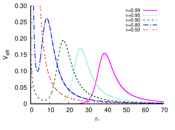
Figure 1: Plot of the effective potential with $r_{*}$ for different values of $\nu$ with $b=2$ and $\ell=2$.

Away from the singularity, for $\nu$ in the range $\left(1/2,1\right)$, the effective potential is characterized by a peak. As $\nu$ decreases from $\nu\approx 1$ to $\nu\approx 1/2$, the height of the potential peak increases and it moves closer to the $r_{*}=0$ surface. For $0<\nu\leq 1/2$, i.e., in the strongly naked singularity regime, the peak vanishes and the potential profile is solely characterized by a potential wall, gradually rising to infinity at the singularity.

IV Time-domain profile and quasinormal modes

In order to study the time evolution of the perturbation, we rewrite the wave equation (18) in terms of the light-cone (null) coordinates, $u=t-r_{*}$ and $v=t+r_{*}$, as,

$$4\frac{\partial^{2}}{\partial u\partial v}\Psi(u,v)+V_{eff}(u,v)\Psi(u,v)=0~{}.$$ (22)

The appropriate discretization scheme to integrate Eq. (22) as proposed by Gundlach, Price and Pullin Gundlach et al. (1994) is,

$$\begin{split}\Psi(N)=&\Psi(W)+\Psi(E)-\Psi(S)\\ &-\Delta^{2}\frac{V_{eff}(W)\Psi(W)+V_{eff}(E)\Psi(E)}{8}+\mathcal{O}\left(\Delta^{4}\right)~{},\end{split}$$ (23)

where we have used the following designations for the points in the $u-v$ plane with step-size $\Delta$: $N=(u+\Delta,v+\Delta)$, $W=(u+\Delta,v)$, $E=(u,v+\Delta)$ and $S=(u,v)$. In the linear regime, the eigenfrequencies of the JNW spacetime are not sensitive to the choice of the initial condition, so, we model the initial perturbation by a Gaussian pulse of width $\sigma$ centred around $v=v_{c}$,

$$\Psi(u=0,v)=e^{-\frac{\left(v-v_{c}\right)^{2}}{2\sigma^{2}}}~{},$$ (24)

and assume the perturbation to vanish at $r_{*}=0$ ,

$$\Psi(r_{*}=0,t)=\Psi(u=v,v)=0,\quad\forall t~{}.$$ (25)

The choice of the boundary condition, given in Eq. (25) deserves some attention. It should be noted that the JNW spacetime fails to be globally hyperbolic due to the naked singularity at $r=b$. A general prescription to define sensible dynamics of the perturbation field (in the linear regime) in such static, nonglobally hyperbolic spacetimes has been suggested by Wald  Wald (1980) (see also Refs. Horowitz and Marolf (1995); Ishibashi and Hosoya (1999); Ishibashi and Wald (2003); Helliwell et al. (2003); Ishibashi and Wald (2004); Gibbons et al. (2005); Cardoso and Cavaglia (2006)). One starts by defining an operator $A$ denoting the spatial (derivative) part of Eq. (18),

$$A=-\frac{d^{2}}{dr_{*}^{2}}+V_{eff}~{}.$$ (26)

The operator $A$ acts on the Hilbert space $\mathcal{H}=L^{2}\left(r_{*},dr_{*}\right)$, of square integrable functions on the static hypersurface $\Sigma$, orthogonal to the unit timelike vector. The existence of a unique self adjoint extension $A_{E}$ of $A$ guarantees unitary dynamical evolution of the perturbation field, which, in our case, corresponds to choosing the appropriate boundary condition at the singularity.

As we approach the singularity, we can write $f(r)\approx b^{-\nu}\left({r-b}\right)^{\nu}$, $\quad h(r)\approx b^{\frac{1+\nu}{2}}(r-b)^{\frac{1-\nu}{2}}$ and the tortoise coordinate, $r_{*}\approx\frac{b^{\nu}}{1-\nu}(r-b)^{1-\nu}$. Close to the singularity, the effective potential reduces to,

$$V_{eff}\left(r_{*}\right)\approx\frac{3}{4r_{*}^{2}}+\mathcal{O}\left(\frac{1}{r_{*}^{\gamma}}\right)~{},$$ (27)

where $\gamma=-\frac{2\nu-1}{1-\nu}<2$ . Assuming,

$$\Psi\left(t,r_{*}\right)=e^{-i\omega t}\Psi\left(r_{*}\right)~{},$$ (28)

we get

$$A\Psi\equiv-\frac{d^{2}\Psi}{dr_{*}^{2}}+V_{eff}\Psi=\omega^{2}\Psi~{},$$ (29)

which at the leading order reduces to

$$-\frac{d^{2}\Psi}{dr_{*}^{2}}+\frac{3}{4r_{*}^{2}}\Psi=\omega^{2}\Psi~{},\quad\mbox{as}\quad r_{*}\rightarrow 0~{}.$$ (30)

The general solution to Eq. (30) is given by,

$$\Psi\sim\mathcal{C}_{1}\left({r_{*}^{-1/2}}+\cdots\right)+\mathcal{C}_{2}\left(r_{*}^{3/2}+\cdots\right)~{},\quad\mbox{as}\quad r_{*}\rightarrow 0.$$ (31)

Equation (31) suggests that for $\Psi$ to be normalizable, we must have $\mathcal{C}_{1}=0$ i.e., $\Psi$ must satisfy

$$r_{*}^{1/2}\Psi\mid_{r_{*}=0}=0~{}.$$ (32)

With the boundary condition (25), one can show that the differential operator $A$ of (29) has a unique Friedrichs extension. Thus the choice of the boundary condition is consistent following Wald’s seminal work Wald (1980). A very brief description of the method is given in Appendix A.

It is important to mention that for scalar field propagation in the Wyman spacetime, which is actually identical with the JNW metric as shown by Virbhadra Virbhadra (1997), the time translation operator also has a unique self-adjoint extension Ishibashi and Hosoya (1999). Chirenti, Saa and Skákala Chirenti et al. (2013), have also shown the uniqueness of the time evolution of scalar fields in the Wyman spacetime.

Using the integration scheme given in Eq. (23), we study the time evolution of the field $\Psi$ along a line of constant $r_{*}$. Figure 2 shows the time evolution of axial perturbation of the JNW space time for different values of the parameter $\nu$. The qualitative features of the ringdown profile are clearly described by the plots.

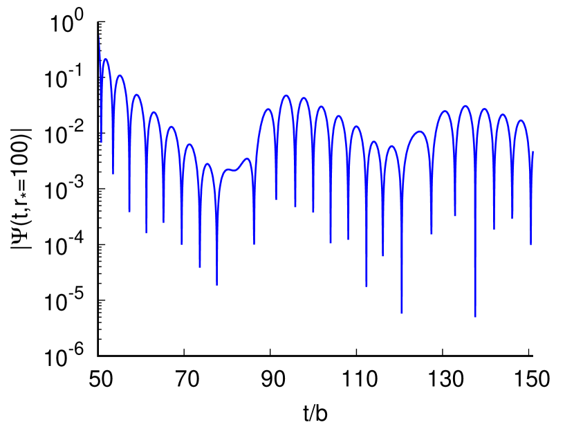
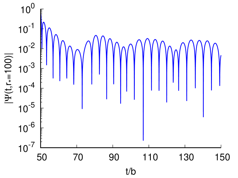
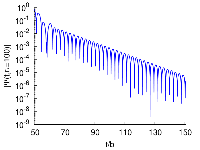
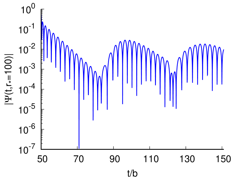
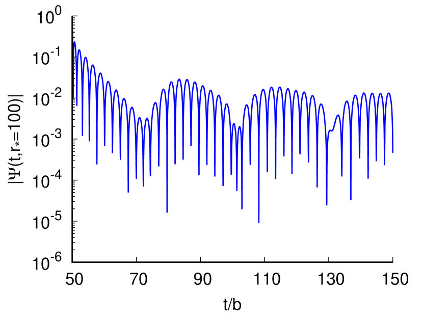
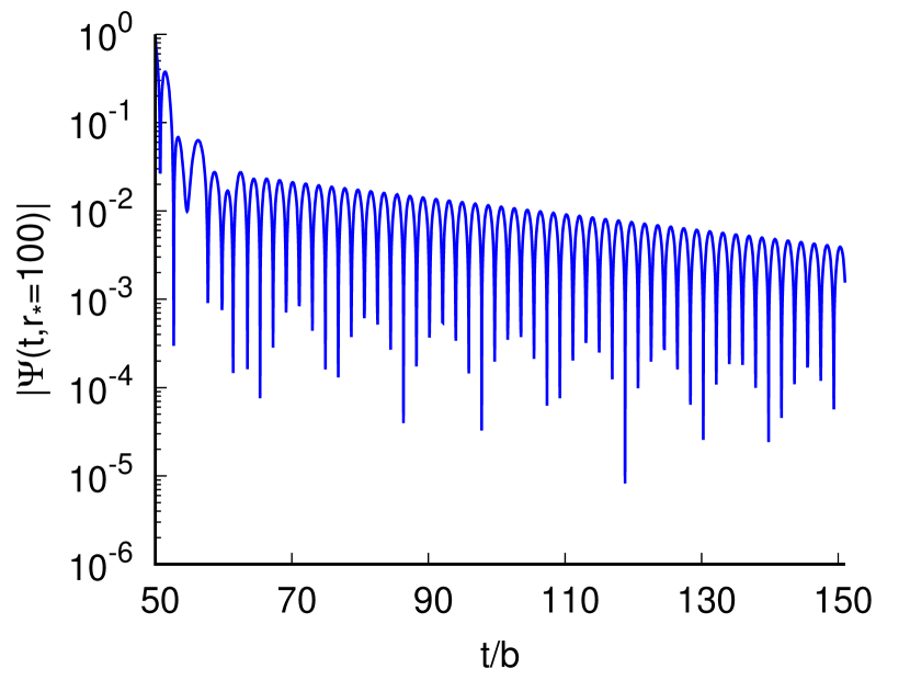
Figure 2: Semilogarithmic plot of the time-domain profiles for axial gravitational perturbation of the JNW spacetime as extracted at $r_{*}=$100 with $b=$2 for $\nu=$0.99, 0.95, 0.75 (from left to right) and $\ell=$2, 3 (from top to bottom). The horizontal axis has been scaled by $b$ to make it dimensionless.

We find that close to the Schwarzschild limit $\left(\nu=1\right)$, when scalar charge $q$ is small, the response of the JNW spacetime is dominated by damped harmonic oscillations, which soon give way to distinctive echoes. The echoes cannot be characterized by a single dominant frequency. However, with the decrease in $\nu$, as the peak of the effective potential moves closer to the wall, the echoes become less prominent and finally, the enveloping oscillation of the echoes align to yield characteristic frequencies of the JNW spacetime.

To extract the characteristic quasinormal mode frequencies from the time-domain profile we use the Prony method of fitting the data via superposition of damped exponentials with some excitation factors Konoplya and Zhidenko (2011); Berti et al. (2007),

$$\Psi(t)\simeq\sum_{j=1}^{p}C_{j}e^{-i\omega_{j}t}~{}.$$ (33)

We provide a brief description of the Prony method in Appendix B. It deserves mention that the usual WKB method of evaluating the quasinormal mode frequencies Schutz and Will (1985); Iyer and Will (1987); Matyjasek and Opala (2017); Konoplya et al. (2019c); Konoplya (2003); Blome and Mashhoon (1984) does not work in the present case. The WKB method is applicable only when the potential function, $U(x,\omega)=V_{eff}(r)-\omega^{2}$ has two turning points, which in general is not the case for the JNW spacetime due to the presence of the infinite potential wall.

Table 1: Fundamental quasinormal mode frequencies (in units of $b$) for axial gravitational perturbation of the JNW spacetime for $\ell=2,3$. The data is indicative of the temporal sequence, QNMs followed by echoes for small $\nu$ and initial outburst (I.O.) followed by QNMs for large $\nu$.

$\nu$	$\omega~{}(\ell=2)$	$\omega~{}(\ell=3)$
$1.00$	$0.3730-0.0891i$	$0.5993-0.0927i$
$0.99$	$0.4066-0.1001i$, echo	$0.6070-0.0940i$, echo
$0.95$	$0.4202-0.1013i$, echo	$0.6362-0.0961i$, echo
$0.86$	I.O. , $0.3404-0.0004i$	$0.7290-0.0968i$, echo
$0.83$	I.O. , $0.4168-0.0033i$	I.O. , $0.5154-0.00003i$
$0.80$	I.O. , $0.4903-0.0122i$	I.O. , $0.6324-0.0004i$
$0.78$	I.O. , $0.5371-0.0235i$	I.O. , $0.7103-0.0019i$
$0.75$	I.O. , $0.6044-0.0492i$	I.O. , $0.8229-0.0105i$
$0.73$	I.O. , $0.6471-0.0725i$	I.O. , $0.8947-0.0233i$

Table 1 shows the fundamental quasinormal mode frequencies of the weakly naked JNW spacetime. The quasinormal modes for the Schwarzschild case ($\nu=1$) correspond to the standard black hole - boundary condition of completely ingoing waves at the horizon and completely outgoing waves at spatial infinity. The quasinormal mode frequency for $\nu=1$ matches with that obtained in Refs. Chandrasekhar and Detweiler (1975); Iyer and Will (1987); Shu and Shen (2005). $\omega$ corresponding to $\nu=0.99,0.95$ for $\ell=2$ and $\nu=0.99,0.95,0.86$ for $\ell=3$ represent the dominant quasinormal mode frequency of the initial oscillatory falloff, characteristic of the potential peak at $r>b$, which later gives rise to echo signals. We see from Table 1 that for a given multipole index, $\ell$, once the scalar charge becomes significantly large and the echoes align ($\nu=0.86-0.73$ for $\ell=2$ and $\nu=0.83-0.73$ for $\ell=3$), both the oscillation frequency and the damping rate of the fundamental quasinormal mode (the real and imaginary parts of the QNM frequency respectively) increase with the decrease of $\nu$. With increasing values of the multipole index the echoes persist for even smaller values of $\nu$.

An important parameter in the analysis of ringdown signal is the quality factor which is defined as the ratio of the real and imaginary parts of the quasinormal mode frequency

$$Q\sim\frac{Real(\omega)}{\left|Im\left(\omega\right)\right|}~{}.$$ (34)

The quality factor for the quasinormal modes of the Schwarzschild black hole and that of the JNW spacetime is shown in Table 2.

Table 2: Quality factor for the fundamental quasinormal mode frequencies for axial gravitational perturbation of the JNW spacetime with $\ell=2,3$.

$\nu$	$Q~{}(\ell=2)$	$Q~{}(\ell=3)$
$1.00$	$4.186$	$6.465$
$0.99$	$4.062$	$6.457$
$0.95$	$4.148$	$6.620$
$0.86$	$851$	$7.531$
$0.83$	$126.303$	$17180$
$0.80$	$40.189$	$1581$
$0.78$	$22.855$	$373.842$
$0.75$	$12.285$	$78.371$
$0.73$	$8.926$	$38.399$

We note from Table 2 that (starting from $\nu=0.99$) for a given multipole index, the quality factor increases with the decrease in $\nu$, reaches a maximum as the echoes in the ring-down profile aligns and then falls off with further decrease in $\nu$.

V Conclusion

The detection of gravitational waves from compact binary coalescence has opened a new window of opportunity to probe the strong field regime of gravity and, hence to test the existence of exotic compact objects. One such horizonless compact object is a naked singularity, which can form as a result of gravitational collapse under suitable initial conditions.

In the present work, we studied the ringdown profile of the Janis-Newman-Winicour naked singularity-spacetime Janis et al. (1968); Wyman (1981); Virbhadra (1997) for an axial gravitational perturbation. We specifically investigated the weakly naked singularity regime where the spacetime is characterized by a photon sphere. At the singularity at $r=b$, the effective potential becomes infinite. For the QNM pertaining to a black hole one has an advantage of picking up boundary conditions elegantly, pure incoming waves at the horizon and pure outgoing waves at large distances. A purely incoming or outgoing mode is not suitable in the present case. For unique time evolution of the perturbation field, we choose null Dirichlet condition at the singularity, consistent with the work of Chirenti, Saa and Skákala Chirenti et al. (2013).

Near the Schwarzschild limit, the initial response of the spacetime is characterized by damped oscillations, reminiscent of the potential peak at $r>b$. At later times, these damped oscillations give rise to distinct echoes. However, as the parameter $\nu$ is decreased, the echoes die down and characteristic quasinormal modes emerge. In the extreme right plots of Fig. 2, both up and down, when $\nu=0.75$, corresponding to $\frac{q}{M}=\frac{\sqrt{7}}{3}$, there are no echoes. Certainly the QNMs are different from the black holes. As the echoes align, the QNM spectrum is dominated by modes with very low damping rate, hence, high quality factor (as evident from Tables 1 and 2 for $\nu=0.86$ for $\ell=2$ and $\nu=0.83$ for $\ell=3$). Thus, the JNW spacetime in this range is an excellent oscillator. With further decrease in $\nu$, both the oscillation frequency and the damping rate of the quasinormal modes increase which in turn reduces the quality factor of the oscillation. It is also important to note that in the entire analysis we do not observe any unstable quasinormal modes with frequency having positive imaginary part.

The existence of echoes in the ringdown signal of the JNW naked singularity is a novel result which categorically differentiates it from a black hole. It deserves mention that Chirenti, Saa and Skákala Chirenti et al. (2013) showed the absence of asymptotically highly damped modes in the Wyman naked singularity Wyman (1981); Virbhadra (1997), but their work was based on the perturbation of a test scalar field whereas the present work is based on the tensor perturbation of the metric. Further investigations may be able to compare the ringdown profile of the JNW spacetime with that of other exotic compact objects such as wormholes which produce similar echoes in the ringdown phase Maggio et al. (2020); Cardoso et al. (2016b); Cardoso and Pani (2017); Mark et al. (2017); Konoplya et al. (2019b); Micchi and Chirenti (2020); Churilova and Stuchlík (2020); Bronnikov and Konoplya (2020); Dutta Roy et al. (2020). Low power echoes may also be produced by black holes, provided, one considers a dramatic deviation from general relativity or effective field theory or both D’Amico and Kaloper (2020). We also plan to extend our analysis to polar perturbations (even parity) as well. In this regard it is also important to note that the perturbation of the scalar field $\Phi$, which does not contribute in the present odd-parity case, will give rise to breathing modes Aneesh et al. (2018) in the QNM spectrum, which results purely from $\delta\Phi$.

Appendix A Friedrichs extension

Whether an operator $A$ admits a self-adjoint extension or not depends on if the so-called the von Neumann criterion is satisfied or not. For a given operator $A$, one looks for the solution for $\phi$ from the equation $A\phi=\pm i\phi$. The dimension of the solution space is called the deficiency index $n$. One will have two values for $n$, namely $n_{\pm}$, corresponding to the two eigenvalues $\pm i$. For $n_{\pm}=0$, there is a unique Friedrichs extension. For nonzero values of the deficiency indices, a self-adjoint extension is still possible if $n_{+}=n_{-}$, although, the uniqueness of the extension is not guaranteed in this case.

The relevant operator in the present work, $A$, as given in Eq. (29), satisfies $n_{\pm}=0$. For an elegant discussion on self-adjoint extension, we refer to Ref. Reed and Simon (1975) (see also Ref.  Pal and Banerjee (2016)).

Appendix B Prony method for extracting QNM frequencies

The fitting of the time-profile data with a sum of damped exponentials can, in general, be performed using standard nonlinear least-squares techniques. However, such fitting is not very accurate Berti et al. (2007). To reduce the squared error over the data, one needs to numerically solve highly nonlinear equations involving sums of the powers of damping coefficients. Such solutions depend critically on the initial guesses for the parameters Marple (1986). Though iterative methods such as Newton’s method or gradient descent algorithms can be used to address the optimization problems, they are computationally very expensive McDonough and Huggins (1968); Evans and Fischl (1973). This led to the development of new class of fitting techniques relying on the method originally developed by Prony in 1795 de Prony (1795).

We start with the assumption that the ringdown begins at $t_{0}=0$ and continues until $t=Nh$, where $N\geq 2p-1$, such that for each $n\in\left(0,N\right)$

$$x_{n}\equiv\Psi(nh)=\sum_{j=1}^{p}C_{j}e^{-i\omega_{j}nh}=\sum_{j=1}^{p}C_{j}z_{j}^{n}~{}.$$ (35)

The Prony method provides an ingenious way to determine $z_{j}$ from the profile data $x_{n}$, thereby allowing to calculate the quasinormal mode frequencies $\omega_{j}$. We define a polynomial $\tilde{A}(z)$ of degree $p$ as

$$\tilde{A}(z)=\displaystyle\prod_{j=1}^{p}(z-z_{j})=\sum_{k=0}^{p}\alpha_{k}z^{p-k},\quad\alpha_{0}=1~{}.$$ (36)

and consider the summation,

$$\sum_{k=0}^{p}\alpha_{k}x_{n-k}=\sum_{k=0}^{p}\alpha_{k}\sum_{j=1}^{p}C_{j}z_{j}^{n-k}=\sum_{j=1}^{p}C_{j}z_{j}^{n-p}\sum_{k=0}^{p}\alpha_{k}z_{j}^{p-k}~{}.$$ (37)

Using Eq. (36) in Eq. (37) we get,

$$\sum_{k=0}^{p}\alpha_{k}x_{n-k}=\sum_{j=1}^{p}C_{j}z_{j}^{n-p}\tilde{A}(z)=0$$ (38)

which can be rewritten as,

$$\sum_{k=1}^{p}\alpha_{k}x_{n-k}=-x_{n}~{}.$$ (39)

Substituting $n=p,\cdots,N$ in Eq. (39), we get $N-P+1\geq p$ linear equations, which can be written in the matrix form,

$$\mathbf{X\alpha}=-\mathbf{x}$$ (40)

where

$$\mathbf{X}=\begin{pmatrix}x_{p-1}&x_{p-2}&\cdots&x_{0}\\ x_{p}&x_{p-1}&\cdots&x_{1}\\ \vdots&\vdots&\ddots&\vdots\\ x_{N-1}&x_{N-2}&\cdots&x_{N-p}\end{pmatrix},\mathbf{\alpha}=\begin{pmatrix}\alpha_{1}\\ \alpha_{2}\\ \vdots\\ \alpha_{p}\end{pmatrix},\mathbf{x}=\begin{pmatrix}x_{p}\\ x_{p+1}\\ \vdots\\ x_{N}\end{pmatrix}~{}.$$ (41)

Equation (40) can be solved in the least-squares sense to determine the unknown coefficient matrix $\mathbf{\alpha}$,

$$\mathbf{\alpha}=-\left(\mathbf{X^{\dagger}X}\right)^{-1}\mathbf{X^{\dagger}x}~{},$$ (42)

where $\mathbf{X^{\dagger}}$ is the Hermitian transpose of $\mathbf{X}$. Having determined the coefficients $\alpha_{k}$ and hence the roots $z_{j}$ of the polynomial $\tilde{A}(z)$ we obtain the quasinormal mode frequencies,

$$\omega_{j}=\frac{i}{h}\ln\left(z_{j}\right)~{}.$$ (43)

References

- Abbott et al. (2016a) B. P. Abbott et al. (LIGO Scientific, Virgo), Phys. Rev. Lett. 116, 241103 (2016a).
- Abbott et al. (2016b) B. Abbott et al. (LIGO Scientific, Virgo), Phys. Rev. Lett. 116, 061102 (2016b).
- Abbott et al. (2017a) B. P. Abbott et al. (LIGO Scientific, Virgo), Phys. Rev. Lett. 118, 221101 (2017a), [Erratum: Phys.Rev.Lett. 121, 129901 (2018)].
- Abbott et al. (2017b) B. P. Abbott et al. (LIGO Scientific, Virgo), Astrophys. J. 851, L35 (2017b).
- Abbott et al. (2017c) B. Abbott et al. (LIGO Scientific, Virgo), Phys. Rev. Lett. 119, 141101 (2017c).
- Abbott et al. (2017d) B. Abbott et al. (LIGO Scientific, Virgo), Phys. Rev. Lett. 119, 161101 (2017d).
- Abbott et al. (2019) B. Abbott et al. (LIGO Scientific, Virgo), Phys. Rev. X 9, 031040 (2019).
- Mann et al. (2019) C. R. Mann, H. Richer, J. Heyl, J. Anderson, J. Kalirai, I. Caiazzo, S. D. Möhle, A. Knee, and H. Baumgardt, Astrophys. J. 875, 1 (2019).
- Martin et al. (2019) R. G. Martin, S. H. Lubow, J. E. Pringle, A. Franchini, Z. Zhu, S. Lepp, R. Nealon, C. J. Nixon, and D. Vallet, Astrophys. J. 875, 5 (2019).
- Zhu et al. (2018) Z. Zhu, M. D. Johnson, and R. Narayan, Astrophys. J. 870, 6 (2018).
- Eckart et al. (2017) A. Eckart, A. Hüttemann, C. Kiefer, S. Britzen, M. Zajaˇcek, C. Lämmerzahl, M. Stöckler, M. Valencia-S, V. Karas, and M. García-Marín, Found. Phys. 47, 553 (2017).
- Abramowicz et al. (2002) M. A. Abramowicz, W. Kluzniak, and J.-P. Lasota, Astron. Astrophys. 396, L31 (2002).
- Unruh and Wald (2017) W. G. Unruh and R. M. Wald, Rept. Prog. Phys. 80, 092002 (2017).
- Mazur and Mottola (2001) P. O. Mazur and E. Mottola, (2001), arXiv:gr-qc/0109035 .
- Mazur and Mottola (2004) P. O. Mazur and E. Mottola, Proc. Natl. Acad. Sci. U.S.A. 101, 9545 (2004).
- Schunck and Mielke (2003) F. E. Schunck and E. W. Mielke, Class. Quantum Grav. 20, R301 (2003).
- Morris et al. (1988) M. S. Morris, K. S. Thorne, and U. Yurtsever, Phys. Rev. Lett. 61, 1446 (1988).
- Damour and Solodukhin (2007) T. Damour and S. N. Solodukhin, Phys. Rev. D 76, 024016 (2007).
- Cardoso et al. (2016a) V. Cardoso, E. Franzin, and P. Pani, Phys. Rev. Lett. 116, 171101 (2016a), [Erratum: Phys.Rev.Lett. 117, 089902 (2016)].
- Mathur (2005) S. D. Mathur, Fortsch. Phys. 53, 793 (2005).
- Barcelo et al. (2011) C. Barcelo, L. Garay, and G. Jannes, Found. Phys. 41, 1532 (2011).
- Barcelo et al. (2015) C. Barcelo, R. Carballo-Rubio, L. J. Garay, and G. Jannes, Class. Quantum Grav. 32, 035012 (2015).
- Holdom and Ren (2017) B. Holdom and J. Ren, Phys. Rev. D 95, 084034 (2017).
- Konoplya et al. (2019a) R. A. Konoplya, C. Posada, Z. Stuchlík, and A. Zhidenko, Phys. Rev. D 100, 044027 (2019a).
- Posada and Chirenti (2019) C. Posada and C. Chirenti, Class. Quantum Grav. 36, 065004 (2019).
- Penrose (2002) R. Penrose, Gen. Rel. Grav. 34, 1141 (2002).
- Liu et al. (2014) Y. Liu, D. Malafarina, L. Modesto, and C. Bambi, Phys. Rev. D 90, 044040 (2014).
- Kiefer and Schmitz (2019) C. Kiefer and T. Schmitz, Phys. Rev. D 99, 126010 (2019).
- Bojowald et al. (2005) M. Bojowald, R. Goswami, R. Maartens, and P. Singh, Phys. Rev. Lett. 95, 091302 (2005).
- Harada et al. (2001) T. Harada, H. Iguchi, K.-i. Nakao, T. P. Singh, T. Tanaka, and C. Vaz, Phys. Rev. D 64, 041501(R) (2001).
- Choptuik (1993) M. W. Choptuik, Phys. Rev. Lett. 70, 9 (1993).
- Joshi and Dwivedi (1993) P. S. Joshi and I. H. Dwivedi, Phys. Rev. D 47, 5357 (1993).
- Waugh and Lake (1988) B. Waugh and K. Lake, Phys. Rev. D 38, 1315 (1988).
- Christodoulou (1984) D. Christodoulou, Commun. Math. Phys. 93, 171 (1984).
- Eardley and Smarr (1979) D. M. Eardley and L. Smarr, Phys. Rev. D 19, 2239 (1979).
- Ori and Piran (1987) A. Ori and T. Piran, Phys. Rev. Lett. 59, 2137 (1987).
- Giambò et al. (2004) R. Giambò, F. Giannoni, G. Magli, and P. Piccione, Gen. Rel. Grav. 36, 1279 (2004).
- Shapiro and Teukolsky (1991) S. L. Shapiro and S. A. Teukolsky, Phys. Rev. Lett. 66, 994 (1991).
- Lake (1991) K. Lake, Phys. Rev. D 43, 1416 (1991).
- Goswami and Joshi (2007) R. Goswami and P. S. Joshi, Phys. Rev. D 76, 084026 (2007).
- Joshi et al. (2002) P. S. Joshi, N. Dadhich, and R. Maartens, Phys. Rev. D 65, 101501(R) (2002).
- Harada et al. (1998) T. Harada, H. Iguchi, and K.-i. Nakao, Phys. Rev. D 58, 041502(R) (1998).
- Banerjee and Chakrabarti (2017) N. Banerjee and S. Chakrabarti, Phys. Rev. D 95, 024015 (2017).
- Bhattacharya et al. (2020) K. Bhattacharya, D. Dey, A. Mazumdar, and T. Sarkar, Phys. Rev. D 101, 043005 (2020).
- Hioki and Maeda (2009) K. Hioki and K.-i. Maeda, Phys. Rev. D 80, 024042 (2009).
- Yang and Li (2016) L. Yang and Z. Li, Int. J. Mod. Phys. D 25, 1650026 (2016).
- Takahashi (2004) R. Takahashi, Astrophys. J. 611, 996 (2004).
- Gyulchev and Yazadjiev (2008) G. N. Gyulchev and S. S. Yazadjiev, Phys. Rev. D 78, 083004 (2008).
- Virbhadra and Ellis (2002) K. S. Virbhadra and G. F. R. Ellis, Phys. Rev. D 65, 103004 (2002).
- Virbhadra et al. (1998) K. Virbhadra, D. Narasimha, and S. Chitre, Astron. Astrophys. 337, 1 (1998).
- Virbhadra and Keeton (2008) K. S. Virbhadra and C. R. Keeton, Phys. Rev. D 77, 124014 (2008).
- Kovács and Harko (2010) Z. Kovács and T. Harko, Phys. Rev. D 82, 124047 (2010).
- Blaschke and Stuchlík (2016) M. Blaschke and Z. c. v. Stuchlík, Phys. Rev. D 94, 086006 (2016).
- Stuchlík and Schee (2010) Z. Stuchlík and J. Schee, Class. Quantum Grav. 27, 215017 (2010).
- Bambi et al. (2009) C. Bambi, K. Freese, T. Harada, R. Takahashi, and N. Yoshida, Phys. Rev. D 80, 104023 (2009).
- Joshi et al. (2011) P. S. Joshi, D. Malafarina, and R. Narayan, Class. Quantum Grav. 28, 235018 (2011).
- Pugliese et al. (2011) D. Pugliese, H. Quevedo, and R. Ruffini, Phys. Rev. D 84, 044030 (2011).
- Gyulchev et al. (2019) G. Gyulchev, P. Nedkova, T. Vetsov, and S. Yazadjiev, Phys. Rev. D 100, 024055 (2019).
- Chowdhury et al. (2012) A. N. Chowdhury, M. Patil, D. Malafarina, and P. S. Joshi, Phys. Rev. D 85, 104031 (2012).
- Sau et al. (2020) S. Sau, I. Banerjee, and S. SenGupta, Phys. Rev. D 102, 064027 (2020).
- Kokkotas and Schmidt (1999) K. D. Kokkotas and B. G. Schmidt, Living Rev. in Rel. 2 (1999), 10.12942/lrr-1999-2.
- Berti et al. (2009) E. Berti, V. Cardoso, and A. O. Starinets, Class. Quantum Grav. 26, 163001 (2009).
- DeBenedictis et al. (2006) A. DeBenedictis, D. Horvat, S. Ilijić, S. Kloster, and K. S. Viswanathan, Class. Quantum Grav. 23, 2303 (2006).
- Chirenti and Rezzolla (2007) C. B. M. H. Chirenti and L. Rezzolla, Class. Quantum Grav. 24, 4191 (2007).
- Pani et al. (2009) P. Pani, E. Berti, V. Cardoso, Y. Chen, and R. Norte, Phys. Rev. D 80, 124047 (2009).
- Ferrari and Kokkotas (2000) V. Ferrari and K. D. Kokkotas, Phys. Rev. D 62, 107504 (2000).
- Chirenti et al. (2012) C. Chirenti, A. Saa, and J. Skákala, Phys. Rev. D 86, 124008 (2012).
- Maggio et al. (2020) E. Maggio, L. Buoninfante, A. Mazumdar, and P. Pani, Phys. Rev. D 102, 064053 (2020).
- Cardoso et al. (2016b) V. Cardoso, S. Hopper, C. F. B. Macedo, C. Palenzuela, and P. Pani, Phys. Rev. D 94, 084031 (2016b).
- Cardoso and Pani (2017) V. Cardoso and P. Pani, Nature Astron. 1, 586 (2017).
- Mark et al. (2017) Z. Mark, A. Zimmerman, S. M. Du, and Y. Chen, Phys. Rev. D 96, 084002 (2017).
- Konoplya et al. (2019b) R. A. Konoplya, Z. Stuchlík, and A. Zhidenko, Phys. Rev. D 99, 024007 (2019b).
- Micchi and Chirenti (2020) L. F. L. Micchi and C. Chirenti, Phys. Rev. D 101, 084010 (2020).
- Churilova and Stuchlík (2020) M. S. Churilova and Z. Stuchlík, Class. Quantum Grav. 37, 075014 (2020).
- Bronnikov and Konoplya (2020) K. A. Bronnikov and R. A. Konoplya, Phys. Rev. D 101, 064004 (2020).
- Dutta Roy et al. (2020) P. Dutta Roy, S. Aneesh, and S. Kar, Eur. Phys. J. C 80, 850 (2020).
- Tsang et al. (2018) K. W. Tsang, M. Rollier, A. Ghosh, A. Samajdar, M. Agathos, K. Chatziioannou, V. Cardoso, G. Khanna, and C. Van Den Broeck, Phys. Rev. D 98, 024023 (2018).
- Janis et al. (1968) A. I. Janis, E. T. Newman, and J. Winicour, Phys. Rev. Lett. 20, 878 (1968).
- Wyman (1981) M. Wyman, Phys. Rev. D 24, 839 (1981).
- Virbhadra (1997) K. S. Virbhadra, Int. J. Mod. Phys. A 12, 4831 (1997).
- Jusufi et al. (2019) K. Jusufi, A. Banerjee, G. Gyulchev, and M. Amir, Eur. Phys. J. C 79, 28 (2019).
- Liu et al. (2018) H. Liu, M. Zhou, and C. Bambi, JCAP 2018, 044 (2018).
- Sadhu and Suneeta (2013) A. Sadhu and V. Suneeta, Int. J. Mod. Phys. D 22, 1350015 (2013).
- Liao et al. (2014) P. Liao, J. Chen, H. Huang, and Y. Wang, Gen. Rel. Grav. 46 (2014).
- Dey et al. (2013) A. Dey, P. Roy, and T. Sarkar, (2013), arXiv:1303.6824 [gr-qc] .
- Chirenti et al. (2013) C. Chirenti, A. Saa, and J. Skákala, Phys. Rev. D 87, 044034 (2013).
- Virbhadra et al. (1997) K. S. Virbhadra, S. Jhingan, and P. S. Joshi, Int. J. Mod. Phys. D 06, 357 (1997).
- Claudel et al. (2001) C.-M. Claudel, K. S. Virbhadra, and G. F. R. Ellis, J. Math. Phys. 42, 818 (2001).
- Regge and Wheeler (1957) T. Regge and J. A. Wheeler, Phys. Rev. 108, 1063 (1957).
- Zerilli (1970) F. J. Zerilli, Phys. Rev. Lett. 24, 737 (1970).
- Rezzolla (2003) L. Rezzolla, ICTP Lect. Notes Ser. 14, 255 (2003).
- Kobayashi et al. (2012) T. Kobayashi, H. Motohashi, and T. Suyama, Phys. Rev. D 85, 084025 (2012).
- Gundlach et al. (1994) C. Gundlach, R. H. Price, and J. Pullin, Phys. Rev. D 49, 883 (1994).
- Wald (1980) R. M. Wald, J. Math. Phys. 21, 2802 (1980).
- Horowitz and Marolf (1995) G. T. Horowitz and D. Marolf, Phys. Rev. D 52, 5670 (1995).
- Ishibashi and Hosoya (1999) A. Ishibashi and A. Hosoya, Phys. Rev. D 60, 104028 (1999).
- Ishibashi and Wald (2003) A. Ishibashi and R. M. Wald, Class. Quantum Grav. 20, 3815 (2003).
- Helliwell et al. (2003) T. Helliwell, D. Konkowski, and V. Arndt, Gen. Rel. Grav. 35, 79 (2003).
- Ishibashi and Wald (2004) A. Ishibashi and R. M. Wald, Class. Quantum Grav. 21, 2981 (2004).
- Gibbons et al. (2005) G. W. Gibbons, S. A. Hartnoll, and A. Ishibashi, Prog. Theor. Phys. 113, 963 (2005).
- Cardoso and Cavaglia (2006) V. Cardoso and M. Cavaglia, Phys. Rev. D 74, 024027 (2006).
- Konoplya and Zhidenko (2011) R. A. Konoplya and A. Zhidenko, Rev. Mod. Phys. 83, 793 (2011).
- Berti et al. (2007) E. Berti, V. Cardoso, J. A. Gonzalez, and U. Sperhake, Phys. Rev. D 75, 124017 (2007).
- Schutz and Will (1985) B. F. Schutz and C. M. Will, Astrophys. J. Lett. 291, L33 (1985).
- Iyer and Will (1987) S. Iyer and C. M. Will, Phys. Rev. D 35, 3621 (1987).
- Matyjasek and Opala (2017) J. Matyjasek and M. Opala, Phys. Rev. D 96, 024011 (2017).
- Konoplya et al. (2019c) R. A. Konoplya, A. Zhidenko, and A. F. Zinhailo, Class. Quantum Grav. 36, 155002 (2019c).
- Konoplya (2003) R. A. Konoplya, Phys. Rev. D 68, 124017 (2003).
- Blome and Mashhoon (1984) H.-J. Blome and B. Mashhoon, Phys. Lett. A 100, 231 (1984).
- Chandrasekhar and Detweiler (1975) S. Chandrasekhar and S. Detweiler, Proc. R. Soc. A 344, 441 (1975).
- Shu and Shen (2005) F.-W. Shu and Y.-G. Shen, Phys. Lett. B 619, 340 (2005).
- D’Amico and Kaloper (2020) G. D’Amico and N. Kaloper, Phys. Rev. D 102, 044001 (2020).
- Aneesh et al. (2018) S. Aneesh, S. Bose, and S. Kar, Phys. Rev. D 97, 124004 (2018).
- Reed and Simon (1975) M. Reed and B. Simon, Fourier Analysis, Self-Adjointness (Academic, 1975).
- Pal and Banerjee (2016) S. Pal and N. Banerjee, J. Math. Phys. 57, 122502 (2016).
- Marple (1986) S. L. Marple, Digital Spectral Analysis: With Applications (Prentice-Hall, Inc., USA, 1986).
- McDonough and Huggins (1968) R. McDonough and W. Huggins, IEEE Trans. Autom. Control 13, 408 (1968).
- Evans and Fischl (1973) A. Evans and R. Fischl, IEEE Trans. Audio Electroacoust. 21, 61 (1973).
- de Prony (1795) G. de Prony, J. l’École Polytechnique 1, 24 (1795).