A Nonmonotone Matrix-Free Algorithm for Nonlinear Equality-Constrained Least-Squares Problems

Abstract

Least squares form one of the most prominent classes of optimization problems, with numerous applications in scientific computing and data fitting. When such formulations aim at modeling complex systems, the optimization process must account for nonlinear dynamics by incorporating constraints. In addition, these systems often incorporate a large number of variables, which increases the difficulty of the problem, and motivates the need for efficient algorithms amenable to large-scale implementations.

In this paper, we propose and analyze a Levenberg-Marquardt algorithm for nonlinear least squares subject to nonlinear equality constraints. Our algorithm is based on inexact solves of linear least-squares problems, that only require Jacobian-vector products. Global convergence is guaranteed by the combination of a composite step approach and a nonmonotone step acceptance rule. We illustrate the performance of our method on several test cases from data assimilation and inverse problems: our algorithm is able to reach the vicinity of a solution from an arbitrary starting point, and can outperform the most natural alternatives for these classes of problems.

65K05, 90C06, 90C30, 90C55.

1 Introduction

This objective is particularly well suited to represent the discrepancy between a model and a set of observations. As a result, such formulations have been successfully applied to a wide range of applications across disciplines [11]. This is not only due to the ubiquitous nature of this problem, but also to the existence of efficient optimization algorithms dedicated to solving this problem by exploiting its specific structure. In particular, the unconstrained setting is particularly well understood: linear least squares can be efficiently solved by exploiting linear algebra solvers [6] while nonlinear least squares are classically tackled using variants of the Gauss-Newton paradigm [21].

In this paper, we consider nonlinear least-squares problems subject to nonlinear constraints of the following form:

(1) $$\begin{array}[]{rl}\displaystyle\min_{x\in\mathbb{R}^{d}}&f(x)\triangleq\frac{1}{2}\|F(x)\|^{2}=\frac{1}{2}\sum_{i=1}^{m}F_{i}(x)^{2},\\ \mbox{s. t.}&C(x)=0,\end{array}$$

where $\|\cdot\|$ will denote the Euclidean norm, $F:\mathbb{R}^{d}\rightarrow\mathbb{R}^{m}$ and $C:\mathbb{R}^{d}\rightarrow\mathbb{R}^{p}$ will be assumed to be nonlinear, potentially nonconvex, continuously differentiable functions. Although one possible approach to solving this problem consists in incorporating the constraints directly into the objective, we are mainly interested in situations in which the constraints represent physical phenomena that drive the behavior of the underlying system, and should not be treated as additional residual functions. Such formulations arise when solving inverse problems [26] in variational modeling for meteorology, such as 4DVAR [27], the dominant data assimilation least-squares formulation used in numerical weather prediction centers. Similar applications include seismic imaging and fluid mechanics [1].

In this work, we aim at combining the Levenberg-Marquardt method [16, 19], one of the most popular algorithms for the solution of nonlinear least squares, with nonlinear programming techniques tailored to solving large-scale equality-constrained problems. Our framework is inspired by inexact trust-region sequential quadratic programming (SQP) [8, 12], which uses inexact computation of a composite step in a careful way that does not jeopardize the convergence guarantees. We combine these techniques with a nonmonotone rule for accepting or rejecting the step, that eschews the use of a penalty function while still guaranteeing global convergence [28]. A nonmonotone rule allows greater flexibility in step acceptance, and thus in practice often converges faster since it accepts a wider range of steps. Our approach builds on previously proposed algorithms of trust-region type, that have a broader scope than least squares. In our case, we do not use second-order derivatives (note that those could be unavailable for algorithmic use), take advantage of the second-order nature of the Gauss-Newton model. We also allow for a “matrix-free” implementation of our algorithm, that only requires access to products of the Jacobian matrices (of both the constraints and objective) with vectors.

The existing literature on Levenberg-Marquardt methods for constrained least squares has mainly focused on establishing local convergence [3, 15] or complexity guarantees [20] for the proposed method. In particular, the work of Izmailov et al. [15] is concerned with local convergence properties of Tikhonov-type regularization algorithms, which requires the use of second derivatives. Meanwhile, other regularization techniques for constrained least squares that do not directly belong to the Levenberg-Marquardt class of methods have recently been proposed, that are also based on the SQP methodology (see [17, 22] and references therein). However, to the best of our knowledge, these approaches are not based on nonmonotone rules, and generally require second-order derivatives.

The rest of this paper is organized as follows. In section 2, we detail the various components of our proposed algorithm, with a focus on inexactness conditions and nonmonotone rules. Section 3 addresses the global convergence of our algorithm. The practical behavior of our method is investigated in Section 4 on problems including nonlinear data assimilation and inverse PDE-constrained optimization. Conclusions and perspectives are finally provided in Section 5.

Notations

Throughout $\|\cdot\|$ will denote the vector or matrix $l_{2}$-norm in any space of the form $\mathbb{R}^{d}$, and $\langle.,.\rangle$ the associated dot product. We will use $A^{\top}$ to for the transpose of the matrix $A$. The identity matrix in $\mathbb{R}^{d\times d}$ will be denoted by $I_{d}$.

2 Algorithmic framework

In this section, we provide a detailed description of the algorithm studied in this paper. Our method combines the Levenberg-Marquardt algorithm with the classical Byrd-Omojokun SQP step [21, Chapter 18] for equality constraints. At every iteration $j$, the method computes a trial step of the form $s_{j}\triangleq n_{j}+t_{j}$, with $n_{j}$ being an inexact quasi-normal step (see Section 2.1) and $t_{j}$ being an inexact tangential step (see Section 2.2). The former aims at improving feasibility, while the latter focuses on lowering the objective value while retaining feasibility. This step is then accepted or rejected depending on nonmonotone decrease requirements: those conditions are described in Section 2.3. The full description of the method is given in Section 2.4.

2.1 Inexact quasi-normal step

Let $\phi(x)\triangleq\tfrac{1}{2}\|C(x)\|^{2}$ denote the constraint violation function at the point $x$. The quasi-normal step is defined as the solution of the following minimization subproblem:

(2) $$\displaystyle\min_{n\in\mathbb{R}^{d}}m_{j}^{c}(n) \triangleq \frac{1}{2}\|C_{j}+J^{c}_{j}n\|^{2}+\frac{1}{2}\gamma_{j}\|n\|^{2},$$

where $C_{j}\triangleq C(x_{j})$ and $J^{c}_{j}\triangleq J^{c}(x_{j})$ denotes the Jacobian of the constraints $C$ at $x_{j}$. The first term in (2) is the Gauss-Newton model of the constraint violation function, while the second term represents a regularization of Levenberg-Marquart type: the regularization parameter $\gamma_{j}$ will be chosen adaptively during the algorithmic process.

For practical purposes (and in particular in a large-scale setting), we consider an approximate solution of the subproblem (2), typically computed using Krylov subspace methods [4, 5]. More precisely, instead of solving  (2) to global optimality, we only require that our inexact quasi-normal step satisfies:

(3) $$m_{j}^{c}(0)-m_{j}^{c}(n_{j})\geq\kappa_{1}\frac{\|C_{j}\|^{2}}{\|J^{c}_{j}\|^{2}+\gamma_{j}}.$$

for some constant $\kappa_{1}>0$. Note that the Cauchy point, i.e. the minimizer of $m_{j}^{c}(n)$ in the subspace spanned by $\nabla m_{j}^{c}(0)$, satisfies the condition (3) under appropriate assumptions [4].

2.2 Inexact tangential step

Having computed the (inexact) quasi-normal step, we now seek an additional step $t_{j}$ that results in a sufficient decrease of the objective function in the tangent space along the level sets of the constraints. We thus consider the Lagrangian function associated with problem (1):

$$\mathcal{L}(x,y) \triangleq f(x)+y^{\top}C(x),~{}~{}~{}~{}~{}~{}~{}y\in\mathbb{R}^{p}.$$

We also define the exact regularized Gauss-Newton model of the Lagrangian at the $j$-th iteration by

(4) $$m_{j}^{l}(s)\;\triangleq\;\frac{1}{2}\|F_{j}+J^{F}_{j}s\|^{2}+y^{\top}_{j}J^{c}_{j}s+\frac{1}{2}\gamma_{j}\|s\|^{2}+y^{\top}_{j}C(x_{j}),$$

where $F_{j}\triangleq F(x_{j})$, $J^{F}_{j}\triangleq J^{f}(x_{j})$ denotes the Jacobian of the residual function $F$ at the current iterate $x_{j}$, and the vector $y_{j}\in\mathbb{R}^{p}$ is a current estimate for the Lagrange multiplier.

The exact tangent step is given as the solution of

(5) $$\begin{array}[]{rl}\displaystyle\min_{t\in\mathbb{R}^{d}}&m_{j}^{l}(n_{j}+t),\\ \text{s.t.}&J^{c}_{j}t=0,\end{array}$$

Note that for any $t\in\mathbb{R}^{d}$, the objective of (5) decomposes as

$$m_{j}^{l}(n_{j}+t)\;=\;m_{j}^{l}(0)+\frac{1}{2}\langle H_{j}n_{j},n_{j}\rangle+\frac{1}{2}\langle H_{j}t,t\rangle+\langle\nabla\mathcal{L}(x_{j},y_{j}),n_{j}\rangle+\langle g_{j},t\rangle.$$

with $H_{j}\triangleq{J_{j}^{F}}^{\top}J_{j}^{F}+\gamma_{j}I_{m}$, $\nabla\mathcal{L}(x_{j},y_{j})={J_{j}^{F}}^{\top}F_{j}+{J^{c}_{j}}^{\top}y_{j}$ and $g_{j}\triangleq\nabla\mathcal{L}(x_{j},y_{j})+H_{j}n_{j}$.

Problem (5) can be reformulated as an unconstrained linear least-squares problem. Indeed, let $W_{j}\triangleq W(x_{j})\in\mathbb{R}^{d\times d}$ denote a projection matrix onto the null space of $J^{c}(x)$: then $W_{j}=W_{j}^{\top}=W_{j}^{2}$ and, for any $t$ such that $J^{c}_{j}t=0$, there exists $w\in\mathbb{R}^{d}$ such that $t=W_{j}w$. Using the reformulation $t=W_{j}w$, the minimization subproblem (5) is thus equivalent to

(6) $$\begin{array}[]{rl}\displaystyle\min_{w\in\mathbb{R}^{d}}&\frac{1}{2}\langle W_{j}^{\top}H_{j}W_{j}w,w\rangle+\langle W_{j}^{\top}g_{j},w\rangle\end{array}$$

To compute the exact tangential step, one can compute a solution $w^{*}$ of (6) then apply $W_{j}$ to obtain the solution $t^{*}=W_{j}w^{*}$ of (5).

One challenge of the approach above is the computation of the matrix $W_{j}$, which can be prohibitive in a large-scale environment. We will thus adopt a matrix-free approach [12]: given $w\in\mathbb{R}^{d}$, the vector $t=W_{j}w$ can be computed by solving the following augmented system

(7) $$\begin{pmatrix}I&{J_{j}^{c}}^{\top}\\ J_{j}^{c}&0\end{pmatrix}\begin{pmatrix}t\\ z\end{pmatrix}=\begin{pmatrix}w\\ 0\end{pmatrix}.$$

As long as ${J^{c}_{j}}$ is surjective, the linear system (7) possesses a solution. An inexact solve of the linear system (7) corresponds to applying an approximation $\widetilde{W}_{j}(\cdot)$ of $W_{j}$ instead of applying the projection matrix $W_{j}$. Therefore, it can be shown [12] that such an inexact solve of (6) corresponds to an exact solve of the following subproblem:

(8) $$\begin{array}[]{rl}\displaystyle\min_{w\in\mathbb{R}^{d}}&\frac{1}{2}\langle H_{j}\widetilde{W}_{j}(w),\widetilde{W}_{j}(w)\rangle+\langle\widetilde{W}_{j}(g_{j}),\widetilde{W}_{j}(w)\rangle,\end{array}$$

which is itself equivalent to

(9) $$\begin{array}[]{rl}\displaystyle\min_{\widetilde{t}\in\mathbb{R}^{d}}&\frac{1}{2}\langle H_{j}{\widetilde{t}},{\widetilde{t}}\rangle+\langle\widetilde{W}_{j}(g_{j}),{\widetilde{t}}\rangle,\end{array}$$

The approximate solutions of (8) and (9) are respectively denoted by $w_{j}$ and . The quality of the inexact step ${\widetilde{t}_{j}}$ will be measured by the inexact model:

$$\widetilde{m}^{l}_{j}(n_{j}+\widetilde{t}_{j})\triangleq m_{j}^{l}(0)+\frac{1}{2}\langle H_{j}n_{j},n_{j}\rangle+\frac{1}{2}\langle H_{j}\widetilde{t}_{j},\widetilde{t}_{j}\rangle+\langle\nabla\mathcal{L}(x_{j},y_{j}),n_{j}\rangle+\langle\widetilde{W}_{j}(g_{j}),\widetilde{t}_{j}\rangle.$$

In order for our step to be sufficiently informative and useful, we will impose the following conditions on the operator $\widetilde{W}_{j}$:

(10a) $$\|\widetilde{W}_{j}(n_{j})-W_{j}n_{j}\| \leq \frac{\xi_{0}}{\gamma^{2}_{j}}$$

(10b) $$\|\widetilde{W}_{j}(g_{j})-W_{j}g_{j}\| \leq \frac{\xi_{1}}{\gamma_{j}}$$

for some $\xi_{0}>0$ and $\xi_{1}>0$. It can be shown [12, Theorem B.1] that the use of inexact linear algebra leads to an approximation $\widetilde{W}_{j}$ of $W_{j}$ such that (10a) and (10b) hold. In our experiments, this corresponds to applying the minres [7] solver to (7) with appropriate choices for the hyperparameters so as to satisfy the conditions described above.

Similarly to the quasi-normal step, we also require $\widetilde{t}_{j}$ to satisfy a fraction of the Cauchy decrease condition on the model $\widetilde{m}^{l}_{j}$, i.e.

(11) $$\widetilde{m}^{l}_{j}(n_{j})-\widetilde{m}^{l}_{j}(n_{j}+\widetilde{t}_{j})\geq\kappa_{2}\frac{\|\widetilde{W}_{j}(g_{j})\|^{2}}{\|J^{F}_{j}\|^{2}+\gamma_{j}},$$

for some constant .

Note that since we consider the use of inexact steps, the vector $\widetilde{t}_{j}=\widetilde{W}_{j}(w_{j})$ might not belong to the null space of $J^{c}_{j}$. Following previous methodology proposed for matrix-free SQP trust region [13, 12], we compute a step $t_{j}$ close to the projection of $\widetilde{t}_{j}$ onto this null space. More precisely, we enforce the following requirement on $t_{j}$:

(12) $$\|t_{j}-W_{j}\widetilde{t}_{j}\|\leq\frac{\xi_{2}}{\gamma_{j}^{2}}.$$

2.3 Nonmonotone acceptance rule

Having computed our inexact steps, we now need to determine whether they are sufficiently promising to deserve acceptance. As in standard SQP trust-region approaches, we compare the decrease predicted by the model and the actual variation produced by the step. Classical monotone frameworks require the actual reduction to be larger than a fraction of the predicted reduction, which may impose unnecessarily severe restrictions on the step [28]. We thus adopt a nonmonotonic step acceptance procedure detailed below.

We first define the predicted reduction and the actual reduction to the constraint violation function by

$$\operatorname{pred}^{c}_{j} \triangleq \phi(x_{j})-m^{c}_{j}(n_{j})=\frac{1}{2}\|C(x_{j})\|^{2}-m^{c}_{j}(n_{j}),$$

$$\operatorname{ared}^{c}_{j} \triangleq \phi(x_{j})-\phi(x_{j}+s_{j})=\frac{1}{2}\|C(x_{j})\|^{2}-\frac{1}{2}\|C(x_{j}+s_{j})\|^{2}.$$

In a monotone framework, the quasi-normal step $n_{j}$ is accepted if $\operatorname{ared}^{c}_{j}$ is larger than a fraction of the predicted reduction $\operatorname{pred}^{c}_{j}$: our nonmonotonic approach requires instead that $\operatorname{rared}^{c}_{j}\geq\rho_{1}\operatorname{pred}^{c}_{j},$ where $\rho_{1}\in(0,1)$, and $\operatorname{rared}^{c}_{j}$ defines the relaxed actual reduction of $\phi$, i.e.

(13) $$\operatorname{rared}^{c}_{j}\;\triangleq\;\frac{1}{2}\max\left\{R_{j},\sum^{\nu^{c}_{j}-1}_{k=0}\mu^{c}_{jk}\|C_{j-k}\|^{2}\right\}-\frac{1}{2}\|C(x_{j}+s_{j})\|^{2},$$

where $\nu\in\mathbb{N}^{*}$, $\mu\in(0,1/m)$, and the quantities $R_{j}$, $\mu_{jk}^{c}$, $\nu^{c}_{j}$ satisfy

$$\nu^{c}_{j}\triangleq\min(j+1,\nu),\,\mu^{c}_{jk}\geq\mu>0,\,\sum^{\nu^{c}_{j}-1}_{k=0}\mu^{c}_{jk}=1,\,R_{j}\geq\|C_{j}\|^{2}$$

In order to compute the quantity $R_{j}$, we rely on an auxiliary procedure described in Algorithm 1. If the constraint violation is not significantly smaller than $\|\hat{g}_{j}\|$, where $\hat{g}_{j}=\widetilde{W}_{j}(g_{j})$ is the reduced gradient, then $R_{j}$ is set to $\|C_{j}\|^{2}$ so as to give preference to steps that improve feasibility. On the other hand, if the constraint violation is much smaller than the norm of the reduced gradient, $R_{j}$ is set to a value larger than $\|C_{j}\|^{2}$ but smaller than a given upper bound $a_{k_{j}}$ where is a slowly decreasing sequence such that $a_{k}>0,\,0<\alpha_{0}\leq\frac{a_{k+1}}{a_{k}}<1,\,\lim_{k\to\infty}a_{k}=0,~{}\mbox{and}\,\sum_{k=0}^{\infty}a^{\eta}_{k}=\infty$, where $4>\eta>4/3$ is a fixed constant (see [28] for details on this procedure).

Algorithm 1 Updating procedure for $R_{j}$

0:  $\alpha>0$, $\beta<1/2$, $k_{j}$ and .  

1:  if $\|C_{j}\|<\min\{\alpha a_{k_{j}},\beta\|\hat{g}_{j}\|\}$ then

2:     $R_{j}=\min\{a^{2}_{k_{j}},\|\hat{g}_{j}\|^{2}\}$.

3:     if $R_{j}\geq\sum^{\nu^{c}_{j}-1}_{k=0}\mu^{c}_{jk}\|C_{j-k}\|^{2}$ then

4:        Set $k_{j+1}=k_{j}+1$.

5:     else

6:        Set $k_{j+1}=k_{j}$.

7:     end if

8:  else

9:     Set $R_{j}=\|C_{j}\|^{2}$ and $k_{j+1}=k_{j}$.

10:  end if

As for the quasi-normal steps, we now introduce a nonmonotone acceptance rule for the tangential step. The predicted reduction for the step $\widetilde{s}_{j}=n_{j}+\tilde{t}_{j}$ is computed as:

$$\operatorname{pred}^{t}_{j}\triangleq\widetilde{m}^{l}_{j}(n_{j})-\widetilde{m}^{l}_{j}(n_{j}+\widetilde{t}_{j})=-\frac{1}{2}\langle H_{j}\widetilde{t}_{j},\widetilde{t}_{j}\rangle-\langle\widetilde{W}_{j}(g_{j}),\widetilde{t}_{j}\rangle,$$

while the predicted reduction for the step $s_{j}=n_{j}+t_{j}$ is defined as

$$\operatorname{pred}^{l}_{j}\triangleq\widetilde{m}^{l}_{j}(0)-\widetilde{m}^{l}_{j}(\widetilde{s}_{j})+\frac{1}{2}\langle\gamma_{j}t_{j}+g_{j},n_{j}-\widetilde{W}_{j}(n_{j})\rangle,$$

The actual reduction of the Lagrangian function $\mathcal{L}$ can be written as

$$\operatorname{ared}^{l}_{j}\triangleq\mathcal{L}(x_{j},y_{j})-\mathcal{L}(x_{j}+s_{j},y_{j})$$

and finally the relaxed (nonmonotone) actual reduction of $\mathcal{L}$ is defined by,

$$\operatorname{rared}^{l}_{j}\triangleq\max\left\{\mathcal{L}(x_{j},y_{j}),\sum^{\nu^{l}_{j}-1}_{k=0}\mu^{l}_{jk}\mathcal{L}(x_{j-k},y_{j-k})\right\}-\mathcal{L}(x_{j}+s_{j},y_{j}),$$

where, similarly to (13), $\mu$ is chosen as in (13), and

$$\nu^{l}_{j}=\min(j+1,\nu^{l}),\,\mu^{l}_{jk}\geq\mu>0,\,\sum^{\nu^{l}_{j}-1}_{k=0}\mu^{l}_{jk}=1.$$

with $\nu^{l}\in\mathbb{N}^{*}$ (Note that for simplicity, we may, and do, in our numerical experiments, choose $\nu^{l}=\nu$).

2.4 Main algorithm

A formal description of the complete algorithm is given in Algorithm 2. Note that it encompasses both exact and inexact variants of our method. Note also that we do not need to specify a procedure to compute the Lagrange multiplier estimate, as those do not play a major role in our global convergence theory. One standard choice, that we adopted in our numerical experiments, is the least-squares multipliers, i.e. the solution to $\min_{y}\|g_{j}-J^{c}_{j}y\|^{2}_{2}$ (note that this subproblem is another unconstrained linear least-squares problem).

Algorithm 2 A nonmonotone matrix-free LM for equality constraints.

0:  $\rho_{1},\rho_{2}\in(0,1)$, $0<\hat{\gamma}_{1}<1<\hat{\gamma}_{2}$, $0<\alpha,\beta<1/2$, $2/3<\xi<1$ $0<\hat{\gamma}<1$, $\alpha_{0}\in(0,1)$, and a sequence . $k_{0}=0$.  

1:  Choose an initial $x_{0}$ and $\gamma_{j}>0$.

2:  for $j=0,1,\ldots$ do

3:     Step 1: Evaluate $F_{j}$, $J^{F}_{j}$, $C_{j}$, $J^{c}_{j}$, $g_{j}$ and a Lagrange multiplier estimate $y_{j}$.

4:     Step 2: Choose $\{\mu^{c}_{jr}\}$ and $\{\mu^{l}_{jr}\}$, then update $R_{j}$ using Algorithm 1.

5:     Step 3: Compute $n_{j}$ such that condition (3) holds and $\widetilde{t}_{j}$ satisfying the conditions (10a), (10b), and (11). Set $\widetilde{s}_{j}=n_{j}+\widetilde{t}_{j}$.

6:     Step 4: Compute $t_{j}$ satisfying the condition (12) and set $s_{j}=n_{j}+t_{j}$ 

7:     Step 5:

8:     if $\operatorname{pred}^{t}_{j}\geq\max\{\operatorname{pred}^{c}_{j},(\operatorname{pred}^{c}_{j})^{\xi}\}\text{ and }\operatorname{pred}^{l}_{j}\geq\rho_{2}\operatorname{pred}^{t}_{j}$ then

9:        if $\operatorname{rared}^{c}_{j}\geq\rho_{1}\operatorname{pred}^{c}_{j}$ and $\operatorname{rared}^{l}_{j}\geq\rho_{1}\operatorname{pred}^{l}_{j}$ then

10:           Set $\gamma_{j}=\max(\gamma_{min},\hat{\gamma}_{1}\gamma_{j})$ and accept the step,i.e., $x_{j+1}=x_{j}+s_{j}$.

11:        else

12:           Set $\gamma_{j}=\hat{\gamma}_{2}\gamma_{j}$ and go to Step 4.

13:        end if

14:     else

15:        if $\operatorname{rared}^{c}_{j}\geq\rho_{1}\operatorname{pred}^{c}_{j}$ then

16:           Set $\gamma_{j}=\max(\gamma_{min},\hat{\gamma}_{1}\gamma_{j})$ and accept the step,i.e., $x_{j+1}=x_{j}+s_{j}$.

17:        else

18:           Set $\gamma_{j}=\hat{\gamma}_{2}\gamma_{j}$ and go to Step 4.

19:        end if

20:     end if

21:  end for

3 Global convergence

3.1 Assumptions and intermediary results

We will establish global convergence of Algorithm 2 under the following standard set of assumptions.

Assumption 3.1.

The sequence $\{x_{j},x_{j}+s_{j}\}$ lies in a compact set $\Omega$.

Assumption 3.2.

Though the rest of the paper, $L^{f}$ and $L_{\phi}$ will denote Lipschitz constants for the gradients of $f$ and $\phi$, respectively. Note that Assumption 3.2 implies that the constraint Jacobian $J^{c}(\cdot)$ is also Lipschitz continuous: through the rest of the paper, $L^{c}$ will be used as the Lipschitz constant for this Jacobian matrix.

Assumptions 3.1 and 3.2 imply that the functions $F$, $C$, $f$, $\phi$ and their derivatives are bounded. In what follows, we will make use of constants $\kappa^{f},\kappa^{\phi},\kappa^{f}_{g},\kappa^{\phi}_{g},\kappa^{F}_{J},\kappa^{c}_{J}$ such that for any $x\in\Omega$, we have

(14a) $$f(x)\leq\kappa^{f},~{}~{}\qquad\phi(x) \leq\kappa^{\phi},$$

(14b) $$\|\nabla f(x)\|\leq\kappa^{f}_{g},\quad\|\nabla\phi(x)\| \leq\kappa^{\phi}_{g},$$

(14c) $$\|J^{F}(x)\|\leq\kappa^{F}_{J},\quad\|J^{c}(x)\| \leq\kappa^{c}_{J}.$$

We will add the following assumption to the above properties.

Assumption 3.3.

There exists $\kappa^{c}_{JJ}>0$ and $\kappa_{W}>0$ such that such that for every index $j$, we have $\left\|\left(J^{c}_{j}{J^{c}_{j}}^{\top}\right)^{-1}\right\|\leq\kappa^{c}_{JJ}$ and $\|\widetilde{W}_{j}(x)\|\leq\kappa_{W}\|x\|$ for any $x$.

Assumption 3.4.

There exists $\kappa_{y}>0$ such that $\|y_{j}\|\leq\kappa_{y}$ for every $j$.

Equipped with these assumptions, we can now state and prove several bounds on algorithmic quantities. To this end, we first state properties of the quasi-normal and tangential steps in Lemma 3.1. Note that those arise from the analysis of the two unconstrained problems (2) and (6), and apply to exact as well as inexact solutions of these subproblems (see [4, Lemma 2.1] and [5, Lemma 5.1] for details).

Lemma 3.1.

Under Assumptions 3.1 to 3.4, for all $j$, one has:

(15a) $$\|n_{j}\| \leq \frac{\|{J^{c}_{j}}^{\top}C_{j}\|}{\gamma_{j}},$$

(15b) $$\|\gamma_{j}n_{j}+{J^{c}_{j}}^{\top}C_{j}\| \leq \frac{\|J^{c}_{j}\|^{2}\|{J^{c}_{j}}^{\top}C_{j}\|}{\gamma_{j}},$$

and

(16a) $$\|\widetilde{t}_{j}\| \leq \frac{\|\widetilde{W}_{j}(g_{j})\|}{\gamma_{j}},$$

(16b) $$\|\gamma_{j}\widetilde{t}_{j}+\widetilde{W}_{j}(g_{j})\| \leq \frac{\|J^{F}_{j}\|^{2}\|\widetilde{W}_{j}(g_{j})\|}{\gamma_{j}}.$$

We can then prove the following series of bounds.

Lemma 3.2.

Under Assumptions 3.1 to 3.4, the sequences $\left\{\left\|g_{j}\right\|\right\}$, $\left\{\gamma_{j}\left\|n_{j}\right\|\right\}$, $\left\{\gamma_{j}\left\|\widetilde{t}_{j}\right\|\right\}$, $\left\{\gamma_{j}\left\|t_{j}\right\|\right\}$, $\left\{\gamma_{j}\left\|\widetilde{s}_{j}\right\|\right\}$, $\left\{\gamma_{j}\left\|s_{j}\right\|\right\}$ and $\left\{\gamma_{j}\|\gamma_{j}\widetilde{t}_{j}+\widetilde{W}_{j}(g_{j})\|\right\}$ are uniformly bounded from above by a positive constant $b_{0}>0$.

Proof 3.3.

Since $g_{j}={J_{j}^{F}}^{\top}F_{j}+{J^{c}_{j}}^{\top}y_{j}+{J^{F}_{j}}^{\top}J^{F}_{j}n_{j}+\gamma_{j}n_{j}$, we have:

$$\|g_{j}\|\;\leq\;\|{J_{j}^{F}}^{\top}F_{j}\|+\|{J^{c}_{j}}\|\|y_{j}\|+\|{J_{j}^{F}}^{\top}J_{j}^{F}+\gamma I_{d}\|\|n_{j}\|.$$

Using the bounds (14) and (15a), we obtain:

$$\|g_{j}\| \leq \kappa_{g}^{f}+\kappa^{c}_{J}\kappa_{y}+{\kappa^{F}_{J}}^{2}\frac{\|{J_{j}^{c}}^{\top}C_{j}\|}{\gamma_{j}}+\|{J_{j}^{c}}^{\top}C_{j}\|\leq\kappa_{g}^{f}+\kappa^{c}_{J}\kappa_{y}+\frac{{\kappa^{F}_{J}}^{2}\kappa_{g}^{\phi}}{\gamma_{min}}+\kappa_{g}^{\phi}\triangleq a_{0}.$$

Using the bound on $\|g_{j}\|$ together with (16a), we obtain:

$$\|\widetilde{t}_{j}\|\leq\frac{\|\widetilde{W}_{j}(g_{j})\|}{\gamma_{j}}\leq\frac{\|\widetilde{W}_{j}\|\|g_{j}\|}{\gamma_{j}}\leq\frac{\kappa_{W}a_{0}}{\gamma_{j}}.$$

Since $\|W_{j}\|=1$ as $W_{j}$ is a projection matrix, and (12) holds, we also have;

$$\|t_{j}\| \leq \|W_{j}\widetilde{t}_{j}\|+\|t_{j}-W_{j}\widetilde{t}_{j}\|\leq\frac{\kappa_{W}a_{0}}{\gamma_{j}}+\frac{\xi_{2}}{\gamma_{j}^{2}}\leq\frac{\kappa_{W}a_{0}+\xi_{2}\gamma_{\min}^{-1}}{\gamma_{j}},$$

Meanwhile, property (15a) guarantees that $\|n_{j}\|\leq\frac{\|{J^{c}_{j}}^{\top}C_{j}\|}{\gamma_{j}}\leq\frac{\kappa_{g}^{\phi}}{\gamma_{j}}$.

Thanks to the three previous bounds on $\|t_{j}\|$, $\|\widetilde{t}_{j}\|$ and $\|n_{j}\|$, we then obtain $\|\widetilde{s}_{j}\|\leq\|n_{j}\|+\|\widetilde{t}_{j}\|\leq\frac{\kappa_{g}^{\phi}+\kappa_{W}a_{0}}{\gamma_{j}}$, as well as

(17) $$\|s_{j}\|\leq\|n_{j}\|+\|t_{j}\|\leq\frac{\kappa_{g}^{\phi}+\kappa_{W}^{2}a_{0}+\xi_{2}\gamma_{\min}^{-1}}{\gamma_{j}}.$$

Finally, property (16b) in Lemma 3.2 gives

$$\|\gamma_{j}\widetilde{t}_{j}+\widetilde{W}_{j}(g_{j})\| \leq \frac{\|J^{F}_{j}\|^{2}\|\widetilde{W}_{j}(g_{j})\|}{\gamma_{j}}\leq\frac{(\kappa^{F}_{J})^{2}\kappa_{W}a_{0}}{\gamma_{j}}.$$

Setting $b_{0}\triangleq\max\{a_{0},\kappa_{W}a_{0},\kappa_{g}^{\phi}+\kappa_{W}a_{0}+\xi_{2}\gamma_{\min}^{-1},(\kappa^{F}_{J})^{2}\kappa_{W}a_{0}\}$ gives the desired result.

The result of Lemma 3.2 allows us to bound the difference between actual and predicted reductions relatively to the regularization parameter.

Lemma 3.4.

Under Assumptions 3.1 to 3.4, there exist positive constants $b_{1}$ and $b_{2}$ such that for every iteration index $j$, one has:

(18a) $$|\operatorname{ared}^{c}_{j}-2\operatorname{pred}^{c}_{j}| \leq \frac{b_{1}}{\gamma_{j}^{2}},$$

(18b) $$|\operatorname{ared}^{l}_{j}-2\operatorname{pred}^{l}_{j}| \leq \frac{b_{2}}{\gamma_{j}^{2}}.$$

Proof 3.5.

To lighten the notation, we will omit the index $j$ in the proof. We begin by proving (18a). Thanks to Assumption 3.2 and the following first-order Taylor expansion of $\phi(\cdot)=\tfrac{1}{2}\|C(\cdot)\|^{2}$, we have:

$$\left|\|C(x+s)\|^{2}-\|C(x)\|^{2}-2C^{\top}J^{c}s-s^{\top}{J^{c}}^{\top}J^{c}s\right|\leq L^{\phi}\|s\|^{2}+\|J^{c}s\|^{2}\leq(L^{\phi}+{\kappa^{c}_{J}}^{2})\|s\|^{2}.$$

Using this formula, we have:

$$|\operatorname{ared}^{c}-2\operatorname{pred}^{c}| = \left|\frac{1}{2}\|C\|^{2}-\frac{1}{2}\|C(x+s)\|^{2}-2\left(\frac{1}{2}\|C\|^{2}-\frac{1}{2}\|C+J^{c}n\|^{2}-\frac{1}{2}\gamma\|n\|^{2}\right)\right|$$

$$= \left|\frac{1}{2}\|C\|^{2}-\frac{1}{2}\|C(x+s)\|^{2}-2C^{\top}J^{c}n-\|J^{c}n\|^{2}-\gamma\|n\|^{2}\right|$$

$$\leq \left|\frac{1}{2}\|C\|^{2}+C^{\top}J^{c}s+\frac{1}{2}s^{\top}{J^{c}}^{\top}J^{c}s-\frac{1}{2}\|C(x+s)\|^{2}\right|$$

$$+ \left|-C^{\top}J^{c}s-\frac{1}{2}s^{\top}{J^{c}}^{\top}J^{c}s-2C^{\top}J^{c}n-\|J^{c}n\|^{2}-\gamma\|n\|^{2}\right|$$

$$\leq \frac{L^{\phi}+{\kappa^{c}_{J}}^{2}}{2}\|s\|^{2}+\left|-C^{\top}J^{c}s-\frac{1}{2}s^{\top}{J^{c}}^{\top}J^{c}s-2C^{\top}J^{c}n-\|J^{c}n\|^{2}-\gamma\|n\|^{2}\right|.$$

Using now the decomposition $s=n+t$ and the fact that $J^{c}W\widetilde{t}=0$, we can reformulate the second term in the last inequality:

$$-C^{\top}J^{c}s-\frac{1}{2}s^{\top}{J^{c}}^{\top}J^{c}s-2C^{\top}J^{c}n-\|J^{c}n\|^{2}-\gamma\|n\|^{2}$$

$$= -C^{\top}J^{c}t-3C^{\top}J^{c}n-\frac{3}{2}\|J^{c}n\|^{2}-\frac{1}{2}\|J^{c}t\|^{2}-\gamma\|n\|^{2}$$

$$= -(C+J^{c}n)^{\top}J^{c}t-n^{\top}(\gamma n+{J^{c}}^{\top}C)-\frac{3}{2}\|J^{c}n\|^{2}-\frac{1}{2}\|J^{c}t\|^{2}$$

$$= -(C+J^{c}n)^{\top}J^{c}(W\widetilde{t}-t)-n^{\top}(\gamma n+{J^{c}}^{\top}C)-\frac{3}{2}\|J^{c}n\|^{2}-\frac{1}{2}\|J^{c}t\|^{2}.$$

Hence, we obtain:

$$|\operatorname{ared}^{c}-2\operatorname{pred}^{c}| \leq \frac{L^{\phi}+{\kappa^{c}_{J}}^{2}}{2}\|s\|^{2}+\|(C+J^{c}n)^{\top}J^{c}\|\|W\widetilde{t}-t\|+\left|n^{\top}(\gamma n+{J^{c}}^{\top}C)\right|$$

$$+\frac{3}{2}\|J^{c}\|^{2}\|n\|^{2}+\frac{1}{2}\|J^{c}\|^{2}\|t\|^{2}$$

$$\leq \frac{L^{\phi}+{\kappa^{c}_{J}}^{2}}{2}\|s\|^{2}+\left(\|C\|+\|J^{c}\|\|n\|\right)\|J^{c}\|\frac{\xi_{2}}{\gamma^{2}}+\|n\|\|\gamma n+{J^{c}}^{\top}C\|$$

$$+\frac{3}{2}\|J^{c}\|^{2}\|n\|^{2}+\frac{1}{2}\|J^{c}\|^{2}\|t\|^{2}$$

$$\leq \frac{(L^{\phi}+{\kappa^{c}_{J}}^{2})b_{0}^{2}}{2\gamma^{2}}+\|J^{c}\|\left(\|C\|+\|J^{c}\|\frac{b_{0}}{\gamma}\right)\frac{\xi_{2}}{\gamma^{2}}+\frac{b_{0}\|J^{c}\|^{2}\|{J^{c}}^{\top}C\|}{\gamma^{2}}+\frac{2b_{0}\|J^{c}\|^{2}}{\gamma^{2}}$$

$$\leq \left[\frac{(L^{\phi}+{\kappa^{c}_{J}}^{2})b_{0}^{2}}{2}+\kappa^{c}_{J}\left(\kappa^{c}+\frac{\kappa^{c}_{J}b_{0}}{\gamma_{\min}}\right)\xi_{2}+b_{0}{\kappa^{c}_{J}}^{2}(\kappa^{\phi}_{g}+2)\right]\frac{1}{\gamma^{2}},$$

where we applied (10b), (15b), Lemma 3.2, (14) and $\gamma\geq\gamma_{\min}$. Hence (18a) holds with $b_{1}=\left[\frac{(L^{\phi}+{\kappa^{c}_{J}}^{2})b_{0}^{2}}{2}+\kappa^{c}_{J}\left(\kappa^{c}+\frac{\kappa^{c}_{J}b_{0}}{\gamma_{\min}}\right)\xi_{2}+b_{0}{\kappa^{c}_{J}}^{2}(\kappa^{\phi}_{g}+2)\right]$.

We now establish (18b). The definition of $\operatorname{pred}^{l}$ gives:

$$\operatorname{pred}^{l} = -\frac{1}{2}\langle Hn,n\rangle-\frac{1}{2}\langle H\widetilde{t},\widetilde{t}\rangle-\langle\nabla_{x}\mathcal{L}(x,y),n\rangle-\langle\widetilde{W}(g),\widetilde{t}\rangle+\frac{1}{2}\langle\gamma t+g,n-\widetilde{W}(n)\rangle$$

$$= \frac{1}{2}\langle Hn,n\rangle-\frac{1}{2}\langle H\widetilde{t},\widetilde{t}\rangle-\langle\nabla_{x}\mathcal{L}(x,y)+Hn,n+W\widetilde{t}\rangle$$

$$-\langle\widetilde{W}(g)-Wg,\widetilde{t}\rangle+\frac{1}{2}\langle\gamma t+g,n-\widetilde{W}(n)\rangle$$

$$= \frac{1}{2}\langle Ht,t\rangle-\frac{1}{2}\langle H\widetilde{t},\widetilde{t}\rangle-\langle\nabla_{x}\mathcal{L}(x,y)+Hn,W\widetilde{t}-t\rangle$$

$$-\langle\nabla_{x}\mathcal{L}(x,y),s\rangle-\frac{1}{2}\langle Hs,s\rangle-\langle\widetilde{W}(g)-Wg,\widetilde{t}\rangle+\frac{1}{2}\langle\gamma t+g,n-\widetilde{W}(n)\rangle,$$

where we first used the formula $g=\nabla_{x}\mathcal{L}(x,y)+Hn$ and $W=W^{\top}$, then $s=t+n$. Consequently,

$$-2\operatorname{pred}^{l} = -\langle Ht,t\rangle+\langle H\widetilde{t},\widetilde{t}\rangle+2\langle\nabla_{x}\mathcal{L}(x,y)+Hn,W\widetilde{t}-t\rangle$$

$$+2\langle\nabla_{x}\mathcal{L}(x,y),s\rangle+\langle Hs,s\rangle+2\langle\widetilde{W}(g)-Wg,\widetilde{t}\rangle-\langle\gamma t+g,n-\widetilde{W}(n)\rangle$$

$$= \langle\nabla_{x}\mathcal{L}(x,y),s\rangle+2\langle g,W\widetilde{t}-t\rangle+2\langle\widetilde{W}(g)-Wg,\widetilde{t}\rangle-\langle\gamma t+g,n-\widetilde{W}(n)\rangle$$

$$+\langle\nabla_{x}\mathcal{L}(x,y),s\rangle-\langle Ht,t\rangle+\langle H\widetilde{t},\widetilde{t}\rangle+\langle Hs,s\rangle$$

$$+\langle g,s\rangle-\langle Hn,s\rangle-\langle Ht,t\rangle+\langle H\widetilde{t},\widetilde{t}\rangle+\langle Hs,s\rangle$$

$$= \langle\nabla_{x}\mathcal{L}(x,y),s\rangle+2\langle g,W\widetilde{t}-t\rangle+2\langle\widetilde{W}(g)-Wg,\widetilde{t}\rangle-\langle\gamma t+g,n-\widetilde{W}(n)\rangle$$

$$+\langle g,s\rangle+\langle Ht,s\rangle-\langle Ht,t\rangle+\langle H\widetilde{t},\widetilde{t}\rangle.$$

Using $H={J^{F}}^{\top}J^{F}+\gamma I_{d}$, we obtain:

$$-2\operatorname{pred}^{l} = \langle\nabla_{x}\mathcal{L}(x,y),s\rangle+2\langle g,W\widetilde{t}-t\rangle+2\langle\widetilde{W}(g)-Wg,\widetilde{t}\rangle-\langle\gamma t+g,n-\widetilde{W}(n)\rangle$$

$$+\langle\gamma t+g,s\rangle+\langle{J^{F}}^{\top}J^{F}t,s\rangle-\langle{J^{F}}^{\top}J^{F}t,t\rangle-\langle\gamma t,t\rangle+\langle{J^{F}}^{\top}J^{F}\widetilde{t},\widetilde{t}\rangle+\langle\gamma\widetilde{t},\widetilde{t}\rangle$$

$$= \langle\nabla_{x}\mathcal{L}(x,y),s\rangle+2\langle g,W\widetilde{t}-t\rangle+2\langle\widetilde{W}(g)-Wg,\widetilde{t}\rangle+\langle\gamma t+g,\widetilde{W}(n)\rangle$$

$$+\langle g,t\rangle+\langle{J^{F}}^{\top}J^{F}t,n\rangle+\langle{J^{F}}^{\top}J^{F}\widetilde{t},\widetilde{t}\rangle+\langle\gamma\widetilde{t},\widetilde{t}\rangle$$

$$= \langle\nabla_{x}\mathcal{L}(x,y),s\rangle+2\langle g,W\widetilde{t}-t\rangle+\langle\widetilde{W}(g)-Wg,\widetilde{t}\rangle+\langle\gamma t+g,\widetilde{W}(n)-Wn\rangle$$

$$\langle\gamma t+g,Wn\rangle+\langle g,t\rangle-\langle Wg,\widetilde{t}\rangle+\langle\gamma\widetilde{t}+\widetilde{W}(g),\widetilde{t}\rangle$$

$$+\langle{J^{F}}^{\top}J^{F}t,n\rangle+\langle{J^{F}}^{\top}J^{F}\widetilde{t},\widetilde{t}\rangle$$

$$= \langle\nabla_{x}\mathcal{L}(x,y),s\rangle+2\langle g,W\widetilde{t}-t\rangle+\langle\widetilde{W}(g)-Wg,\widetilde{t}\rangle+\langle\gamma t+g,\widetilde{W}(n)-Wn\rangle$$

$$\langle W(\gamma t+g),n\rangle+\langle g,t-W\widetilde{t}\rangle+\langle\gamma\widetilde{t}+\widetilde{W}(g),\widetilde{t}\rangle+\langle{J^{F}}^{\top}J^{F}t,n\rangle+\langle{J^{F}}^{\top}J^{F}\widetilde{t},\widetilde{t}\rangle$$

$$= \langle\nabla_{x}\mathcal{L}(x,y),s\rangle+\langle g,W\widetilde{t}-t\rangle+\langle\widetilde{W}(g)-Wg,\widetilde{t}\rangle+\langle\gamma t+g,\widetilde{W}(n)-Wn\rangle$$

$$\langle W(\gamma t+g),n\rangle+\langle\gamma\widetilde{t}+\widetilde{W}(g),\widetilde{t}\rangle+\langle{J^{F}}^{\top}J^{F}t,n\rangle+\langle{J^{F}}^{\top}J^{F}\widetilde{t},\widetilde{t}\rangle,$$

where the line before last is obtained using $W^{\top}=W$. As a result,

$$|\operatorname{ared}^{l}-2\operatorname{pred}^{l}| = |\mathcal{L}(x)-\mathcal{L}(x+s)-2\operatorname{pred}^{l}|$$

$$\leq |\mathcal{L}(x)+\langle\nabla_{x}\mathcal{L}(x,y),s\rangle-\mathcal{L}(x+s)|+\|g\|\|W\widetilde{t}-t\|$$

$$+\|\widetilde{W}(g)-Wg\|\|\widetilde{t}\|+(\gamma\|t\|+\|g\|)\|\widetilde{W}(n)-Wn\|$$

$$+\|W(\gamma t+g)\|\|n\|+\|\gamma\widetilde{t}+\widetilde{W}(g)\|\|\widetilde{t}\|.+\|J^{F}\|^{2}\left(\|t\|\|n\|+\|\widetilde{t}\|^{2}\right)$$

By Assumptions 3.2 and 3.4, we have

$$\left|\mathcal{L}(x,y)+\langle\nabla_{x}\mathcal{L}(x,y),s\rangle-\mathcal{L}(x+s,y)\right| \leq \left|f(x+s)-f(x)-\nabla f(x)^{\top}s\right|$$

$$+\|y\|\left\|C(x+s)-C(x)-{J^{c}}^{\top}s\right\|$$

(19) $$\left|\mathcal{L}(x,y)+\langle\nabla_{x}\mathcal{L}(x,y),s\rangle-\mathcal{L}(x+s,y)\right| \leq \frac{L^{f}+\kappa_{y}L^{c}}{2}\|s\|^{2}.$$

Therefore,

(20) $$|\operatorname{ared}^{l}-2\operatorname{pred}^{l}| \leq \frac{L^{f}+\kappa_{y}L^{c}}{2}\|s\|^{2}+\|g\|\|W\widetilde{t}-t\|$$

$$+\|\widetilde{W}(g)-Wg\|\|\widetilde{t}\|+(\gamma\|t\|+\|g\|)\|\widetilde{W}(n)-Wn\|$$

$$+\|W(\gamma t+g)\|\|n\|+\|\gamma\widetilde{t}+\widetilde{W}(g)\|\|\widetilde{t}\|.+\|J^{F}\|^{2}\left(\|t\|\|n\|+\|\widetilde{t}\|^{2}\right),$$

where the last line comes from (3.5). To conclude, we need the result below, that uses the properties $W^{2}=W=W^{\top}$ and $\|W\|=1$ of the projection matrix $W$. One has:

$$\|W(\gamma t+g)\| = \|\gamma W(t-W\widetilde{t})+W(\gamma\widetilde{t}+\widetilde{W}(g))+W(Wg-\widetilde{W}(g))\|$$

$$\leq \gamma\|t-W\widetilde{t}\|+\|\gamma\widetilde{t}+\widetilde{W}(g)\|+\|Wg-\widetilde{W}(g)\|$$

(21) $$\|W(\gamma t+g)\| \leq \frac{\xi_{2}}{\gamma}+\frac{b_{0}}{\gamma}+\frac{\xi_{1}}{\gamma}.$$

where the last line uses (12), Lemma 3.2 and (10b).

Using (3.5) as well as (10a),(10b),(12), the bounds from Lemma 3.2 and (3.5), we can bound all the terms in (20) and we arrive at:

$$|\operatorname{ared}^{l}-2\operatorname{pred}^{l}| \leq \frac{(L^{f}+\kappa_{y}L^{c})b_{0}^{2}}{2\gamma^{2}}+\frac{b_{0}\xi_{2}}{\gamma^{2}}+\frac{b_{0}\xi_{1}}{\gamma^{3}}+\frac{2b_{0}\xi_{0}}{\gamma^{2}}$$

$$+\frac{2b_{0}(\xi_{2}+b_{0}+\xi_{1})}{\gamma^{2}}+\frac{b_{0}^{2}}{\gamma^{2}}+\frac{2{\kappa^{F}_{J}}^{2}b_{0}^{2}}{\gamma^{2}}.$$

Using $\gamma\geq\gamma_{\min}$, we obtain $|\operatorname{ared}^{l}-2\operatorname{pred}^{l}|\leq\frac{b_{2}}{\gamma^{2}}$ with
$b_{2}=b_{0}\left(\frac{(L^{f}+\kappa_{y}L^{c}+6+4\kappa^{F}_{J})b_{0}}{2}+3\xi_{2}+\frac{\xi_{1}+2\gamma_{\min}}{\gamma_{\min}}+2\xi_{0}\right)$.

3.2 Main convergence results

We now present a global convergence analysis for our framework, that is inspired by the analysis of nonmonotone trust-region algorithms without penalty function [28].

We first establish that, if the method has not converged yet, Algorithm 2 eventually computes and accepts a step for a sufficiently large $\gamma_{j}$. This is the purpose of the next lemma, which is similar to [28, Lemma 1] but adapted to our inexact context.

Lemma 3.6.

Under Assumptions 3.1-3.4, let $\epsilon>0$, and suppose that the $j$-th iterate of Algorithm 2 is such that $\|C_{j}\|+\|\widetilde{W}_{j}(g_{j})\|>2\epsilon$. Then, there exists $\bar{\gamma}>0$ (depending on $\epsilon$, $\|C_{j}\|$ and $a_{k_{j}}$) such that the step $s_{j}$ is accepted whenever $\gamma_{j}>\bar{\gamma}$.

Proof 3.7.

Since $\|C_{j}\|+\|\widetilde{W}_{j}(g_{j})\|>2\epsilon$, one of the two quantities $\|C_{j}\|$ and $\|\widetilde{W}_{j}(g_{j})\|$ must be larger than $\epsilon$. We thus consider two cases.

Case 1: Suppose that $\|C_{j}\|>\epsilon$. By combining (3) and (14c), we then have that $\operatorname{pred}^{c}_{j}\geq\kappa_{1}\frac{\epsilon^{2}}{{\kappa^{c}_{J}}^{2}+\gamma_{j}},$ while Lemma 3.4 guarantees that $|\operatorname{ared}^{c}_{j}-2\operatorname{pred}^{c}_{j}|\leq\frac{b_{1}}{\gamma_{j}^{2}}$. Hence,

$$\left|2-\frac{\operatorname{ared}^{c}_{j}}{\operatorname{pred}^{c}_{j}}\right| = \left|\frac{2\operatorname{pred}^{c}_{j}}{\operatorname{pred}^{c}_{j}}-\frac{\operatorname{ared}^{c}_{j}}{\operatorname{pred}^{c}_{j}}\right|\leq\frac{b_{1}}{\kappa_{1}\epsilon^{2}}\frac{{\kappa_{J}^{c}}^{2}+\gamma_{j}}{\gamma_{j}^{2}}\rightarrow 0\mbox{~{}~{}~{}~{}~{}as~{}~{}}\gamma_{j}\to\infty.$$

Thus there exists $\bar{\gamma}_{1}>0$ such that if $\gamma_{j}\geq\bar{\gamma}_{1}>0$, then $\operatorname{rared}^{c}_{j}\geq\operatorname{ared}^{c}_{j}\geq\rho_{1}\operatorname{pred}^{c}_{j}$. If either $\operatorname{pred}^{t}_{j}<\max\{\operatorname{pred}^{c}_{j},(\operatorname{pred}^{c}_{j})^{\xi}\}$ or $\operatorname{pred}^{l}_{j}<\rho_{2}\operatorname{pred}^{t}_{j}$, we know that the step will be accepted. Otherwise (i.e. $\operatorname{pred}^{t}_{j}\geq\max\{\operatorname{pred}^{c}_{j},(\operatorname{pred}^{c}_{j})^{\xi}\}$ and $\operatorname{pred}^{l}_{j}\geq\rho_{2}\operatorname{pred}^{t}_{j}$):

$$\operatorname{pred}^{l}_{j}\geq\rho_{2}\operatorname{pred}^{t}_{j}\geq\rho_{2}\operatorname{pred}^{c}_{j}\geq\rho_{2}\kappa_{1}\frac{\epsilon^{2}}{{\kappa^{c}_{J}}^{2}+\gamma_{j}}.$$

Since by Lemma 3.4, $|\operatorname{ared}^{l}_{j}-2\operatorname{pred}^{l}_{j}|\leq\frac{b_{2}}{\gamma_{j}^{2}}$, we can use the same argument than above to show that there exists $\bar{\gamma}_{2}$ such that $\operatorname{rared}_{j}^{l}\geq\operatorname{ared}^{l}_{j}\geq\rho_{1}\operatorname{pred}^{l}_{j}$ for $\gamma_{j}\geq\bar{\gamma}_{2}$, and thus the step is accepted.

Case 2: Suppose now that $\|\widetilde{W}_{j}(g_{j})\|>\epsilon$. By (11) and (14c), this implies that $\operatorname{pred}^{t}_{j}\geq\kappa_{2}\frac{\epsilon^{2}}{{\kappa^{F}_{J}}^{2}+\gamma_{j}}$. We consider two subcases.
Case 2.1: If $\operatorname{pred}^{c}_{j}\geq\operatorname{pred}^{t}_{j}$, we have $\operatorname{pred}^{c}_{j}\geq\kappa_{2}\frac{\epsilon^{2}}{{\kappa^{F}_{J}}^{2}+\gamma_{j}}$ and the same argument than in Case 1 can be employed to guarantee that the step is accepted for $\gamma_{j}\geq\bar{\gamma}_{3}$ for a certain $\bar{\gamma}_{3}>0$.
Case 2.2: If $\operatorname{pred}^{c}_{j}<\operatorname{pred}^{t}_{j}$, then the only condition required for step acceptance is that $\operatorname{rared}^{c}_{j}\geq\rho_{1}\operatorname{pred}^{c}_{j}$. Defining $\epsilon_{k_{j}}=\min(\alpha a_{k_{j}},\beta\epsilon)$ (see Algorithm 1, we then compare $\epsilon_{k,j}$ and $\|C_{j}\|$. If $\|C_{j}\|>\epsilon_{k_{j}}$, the reasoning of Case 1 (with $\epsilon_{k,j}$ playing the role of $\epsilon$) guarantees that there exists $\bar{\gamma}_{4}>0$ such that the step is accepted when $\gamma_{j}>\bar{\gamma}_{4}$. On the other hand, if $\|C_{j}\|\leq\epsilon_{k_{j}}$, we have $R_{j}\geq\min(a_{k_{j}}^{2},\epsilon^{2})\geq 4\epsilon_{k_{j}}^{2}$, which then gives:

$$\operatorname{rared}^{c}_{j}\geq\frac{1}{2}R_{j}-\frac{1}{2}\|C(x_{j}+s_{j})\|^{2} \geq \frac{1}{2}R_{j}-\frac{1}{2}\|C(x_{j})\|^{2}-{J^{c}_{j}}^{\top}s_{j}-\frac{L^{c}}{2}\|s_{j}\|^{2}$$

$$\geq \frac{3}{2}\epsilon_{k,j}^{2}-\frac{\kappa^{c}_{J}b_{0}}{\gamma_{j}}-\frac{L^{c}b_{0}^{2}}{2\gamma_{j}^{2}},$$

where the last inequality comes from (14c) and Lemma 3.2. Thus there exists $\bar{\gamma}_{5}>0$ such that $\operatorname{rared}^{c}_{j}\geq\rho_{1}\epsilon_{k_{j}}^{2}$ for $\gamma_{j}>\bar{\gamma}_{5}$: since $\operatorname{pred}^{c}_{j}\leq\frac{1}{2}\|C_{j}\|^{2}\leq\frac{1}{2}\epsilon_{k_{j}}^{2}$ by definition, we then have $\operatorname{rared}^{c}_{j}\geq\rho_{1}\operatorname{pred}^{c}_{j}$, and the step is accepted.

Letting $\bar{\gamma}=\max\{\bar{\gamma}_{1},\bar{\gamma}_{2},\bar{\gamma}_{3},\bar{\gamma}_{4},\bar{\gamma}_{5}\}$ finally leads to the desired result.

The remainder of our analysis relies on several arguments that are identical to the trust-region setting, which we restate below (see [28, Lemmas 2-5] for proofs). The analysis relies on considering the steps that have been accepted: for this purpose, the subscript _j,a will refer to quantities related to the $j$-th iteration at which the step was accepted (e.g. $s_{j,a}$ denotes the accepted step at iteration $j$).

Lemma 3.8.

Under Assumptions 3.1-3.4, suppose that there exists $\hat{j}\geq 0$ such that for all $j\geq\hat{j}$, we have $\operatorname{rared}^{c}_{j,a}=\max\left\{\|C_{j}\|^{2},\sum^{\nu^{c}_{j}-1}_{k=0}\mu^{c}_{jk}\|C_{j-k}\|^{2}\right\}-\|C_{j+1}\|^{2}.$ Then, for all $j\geq\hat{j}$, $\|C_{j+1}\|^{2}\leq\max_{\hat{j}-\nu^{c}_{j}<l\leq\hat{j}}R_{l}-\rho_{1}\sum_{r=\hat{j}}^{j}\mu^{\min\{j-r,\nu\}}\operatorname{pred}^{c}_{r,a}.$

Lemma 3.9.

Under Assumptions 3.1 to 3.4, suppose that there exists $\hat{j}\geq 0$ such that, for all $j\geq\hat{j}$, we have $\operatorname{rared}^{l}_{j,a}+\mathcal{L}(x_{j+1},y_{j})-\mathcal{L}(x_{j+1},y_{j+1})\geq\frac{\rho_{1}}{2}\operatorname{pred}^{l}_{j,a}$.
Then, for all $j\geq\hat{j}$,

$$|\mathcal{L}(x_{j+1},y_{j+1})|\leq\max_{\hat{j}-\nu^{l}_{j}<l\leq\hat{j}}\mathcal{L}(x_{l},y_{l})-\frac{\rho_{1}}{2}\sum_{r=\hat{j}}^{j}\mu^{\min(j-r,\nu)}\operatorname{pred}^{l}_{r,a}.$$

Lemma 3.10.

Let Assumptions 3.1-3.4 hold. If, at the $j$-th iteration of Algorithm 2, Algorithm 1 performs the update $k_{j+1}=k_{j}+1$, then $\|C_{j^{\prime}}\|\leq\frac{1}{\sqrt{\mu}}a_{k_{j}}$ for all $j^{\prime}\geq j$. In particular, for all iterations $j$ with $k_{j}\geq 1$, one has $\|C_{j}\|\leq\frac{a_{k_{j}}}{\sqrt{\mu}\alpha_{0}}.$

Lemma 3.11.

Let Assumptions 3.1-3.4 hold. If for infinitely many iterations,

$$\operatorname{rared}^{c}_{j,a}\neq\max\left\{\|C_{j}\|^{2},\sum_{r=0}^{v^{c}_{j}-1}\mu^{c}_{jr}\|C_{j-r}\|^{2}\right\}-\|C_{j+1}\|^{2}$$

holds, then $k_{j}\to\infty$ and $\|C_{j}\|\to 0$.

We now have all the ingredients to establish global convergence of our framework. We begin by showing that the sequence of iterates is asymptotically feasible.

Theorem 3.12.

Under Assumptions 3.1-3.4, if Algorithm 2 does not terminate finitely, then $\lim_{j\to\infty}\|C_{j}\|=0.$

Proof 3.13.

The proof proceeds by contradiction. Suppose that $\limsup_{j\to\infty}\|C_{j}\|>0$. Then, by Lemma 3.11, there exists $\hat{j}$ such that for $j\geq\hat{j}$,

$$\operatorname{rared}^{c}_{j,a}=\max\left\{\|C_{j}\|^{2},\sum_{r=0}^{v^{c}_{j}-1}\mu^{c}_{jr}\|C_{j-r}\|^{2}\right\}-\|C_{j+1}\|^{2}$$

which implies by Lemma 3.8:

$$\|C_{j+1}\|^{2}\leq M_{\hat{j}}-\rho_{1}\sum_{r=\hat{j}}^{j}\mu^{\min\{j-r,\nu\}}\operatorname{pred}^{c}_{r,a}~{}~{}\text{where}~{}~{}M_{\hat{j}}=\max_{\hat{j}-\nu^{c}_{j}<l\leq\hat{j}}R_{l},$$

Since $\mu\in(0,1)$, we thus get for all $j\geq\hat{j}$,

(22) $$\|C_{j+1}\|^{2}\leq M_{\hat{j}}-\rho_{1}\mu^{\nu}\sum_{r=\hat{j}}^{j}\operatorname{pred}^{c}_{r,a}.$$

We first consider the case $\liminf_{j\to\infty}\|C_{j}\|\neq 0$: in that situation, there exists an $\epsilon$ for which $\|C_{j}\|\geq\epsilon$ for $j\geq\hat{j}$. By (3), this implies

$$\operatorname{pred}^{c}_{j,a}\geq\kappa_{1}\frac{\epsilon^{2}}{(\kappa^{c}_{J})^{2}+\gamma_{j,a}},$$

which, combined with (22), leads to

(23) $$\sum_{j=\hat{j}}^{\infty}\frac{1}{(\kappa^{c}_{J})^{2}+\gamma_{j,a}}<\infty\;\Rightarrow\;\lim_{j\to\infty}\gamma_{j,a}=+\infty.$$

Since $\|C_{j}\|\geq\epsilon$, similarly to Case 1 in the proof of Lemma 3.6, we can show that for sufficiently large $\gamma_{j}$, the step must be accepted. This, together with the step acceptance rule, guarantees that there exists an upper bound for $\gamma_{j,a}$, which contradicts (23). Thus, we must have $\liminf_{j\to\infty}\|C_{j}\|=0$.

Because we assumed that $\limsup_{j\to\infty}\|C_{j}\|\neq 0$, for any $\epsilon>0$, there exists a subsequence $\{\underline{j}\}$ such that $\|C_{\underline{j}}\|\geq 2\epsilon$. Since we just established $\liminf_{j\to\infty}\|C_{j}\|=0$, for each index $\underline{j}$ of that subsequence, there exists $\overline{j}>\underline{j}$ such that $\|C_{\overline{j}+1}\|<\epsilon$ and $\|C_{j}\|\geq\epsilon$ for $j=\underline{j},...,\overline{j}$. For $j=\underline{j},...,\overline{j}$, it thus holds that

(24) $$\operatorname{pred}^{c}_{j,a}(n_{j,a})\geq\kappa_{1}\frac{\epsilon^{2}}{(\kappa^{c}_{J})^{2}+\gamma_{j,a}},\,j=\underline{j},...,\overline{j}.$$

On the other hand, by (22) and our assumption that $\limsup_{j\to\infty}\|C_{j}\|\neq 0$, we have that $\sum_{j=\underline{j}}^{\overline{j}}\operatorname{pred}^{c}_{j,a}\to 0\text{ for }\underline{j}\to\infty.$ Meanwhile, Lemma 3.2 guarantees that $\|s_{j,a}\|\leq\frac{b_{0}}{\gamma_{j,a}}$, so that

$$\|x_{\overline{j}+1}-x_{\underline{j}}\| \leq \sum_{j=\underline{j}}^{\overline{j}}\frac{b_{0}}{\gamma_{j,a}}=b_{0}\sum_{j=\underline{j}}^{\overline{j}}\frac{(\kappa^{c}_{J})^{2}+\gamma_{j,a}}{\gamma_{j,a}((\kappa^{c}_{J})^{2}+\gamma_{j,a})}$$

$$\leq \frac{b_{0}}{\epsilon^{2}\kappa_{1}}\left(\frac{(\kappa^{c}_{J})^{2}}{\gamma_{\min}}+1\right)\sum_{j=\underline{j}}^{\overline{j}}\operatorname{pred}^{c}_{j,a}\to 0\text{ for }\underline{j}\to\infty,$$

where the last inequality comes from (24). By Assumption 3.2, we then obtain

$$\epsilon=2\epsilon-\epsilon\leq\|C_{\overline{j}+1}\|-\|C_{\underline{j}}\|\leq\|C_{\overline{j}+1}-C_{\underline{j}}\|\leq 2\|J^{c}_{j}\|\|\|x_{\overline{j}+1}-x_{\underline{j}}\|+L^{c}\|x_{\overline{j}+1}-x_{\underline{j}}\|,$$

and the right-hand side goes to $0$ as $\underline{j}\to\infty$. We have thus reached a contradiction, from which we conclude that $\lim_{j\to\infty}\|C_{j}\|=0$.

We now establish convergence towards a certain form of stationarity.

Theorem 3.14.

Under the assumptions of Theorem 3.12, the sequence of iterates of Algorithm 2 is such that $\liminf_{j\to+\infty}\|\widetilde{W}_{j}(g_{j})\|=0.$

Proof 3.15.

We again seek a contradiction by assuming that there exists $\epsilon>0$ such that $\liminf_{j\to+\infty}\|\widetilde{W}_{j}(g_{j})\|\geq\epsilon$. From Lemma 3.6, we know that, in that case, the trial step is always accepted if $\gamma_{j}$ is sufficiently large. By the updating rule for $\gamma_{j}$, this implies that the sequence $\{\gamma_{j}\}$ is bounded from above, i.e. there exists $\gamma_{M}>0$ such that $\gamma_{j}<\gamma_{M}$ for all $j$. From (11), we then have $\operatorname{pred}^{t}_{j,a}\geq\kappa_{2}\frac{\epsilon^{2}}{(\kappa^{f}_{g})^{2}+\gamma_{M}}$: since $\operatorname{pred}^{c}_{j,a}\leq\|C_{j,a}\|^{2}\to 0$ thanks to Theorem 3.12, for $j$ sufficiently large, we must have eventually $\operatorname{pred}^{t}_{j,a}>\operatorname{pred}^{c}_{j,a}$. Furthermore, using Lemma 3.2,

$$|\operatorname{pred}^{l}_{j,a}-\operatorname{pred}^{t}_{j,a}|\leq|\widetilde{m}^{l}_{j}(0)-\widetilde{m}^{l}_{j}(n_{j,a})|+\frac{1}{2}\|\gamma_{j}t_{j,a}+g_{j,a}\|\|n_{j,a}-\widetilde{W}_{j,a}(n_{j,a})\|$$

$$\leq \frac{1}{2}\left(\|J^{F}_{j}\|^{2}+\gamma_{j,a}\right)\|n_{j,a}\|^{2}+\left(\|{J^{f}_{j,a}}^{\top}F_{j,a}\|+\|J^{c}_{j,a}\|\|y_{j,a}\|\right)\|n_{j,a}\|+b_{0}(1+\kappa_{W})\|n_{j,a}\|$$

$$\leq \frac{1}{2}((\kappa^{f}_{J})^{2}+\gamma_{M})\|n_{j,a}\|^{2}+(\kappa^{f}_{J}\kappa^{f}+\kappa^{c}_{g}\kappa_{y}+b_{0}(1+\kappa_{W}))\|n_{j,a}\|$$

$$\leq \frac{1}{2}((\kappa^{f}_{J})^{2}+\gamma_{M})\left(\frac{\|J^{c}_{j,a}\|\|C_{j,a}\|}{\gamma_{j,a}}\right)^{2}+(\kappa^{f}_{g}\kappa^{f}+\kappa^{c}_{g}\kappa_{y}+b_{0}(1+\kappa_{W}))\frac{\|J^{c}_{j,a}\|\|C_{j,a}\|}{\gamma_{j,a}}$$

$$\leq \frac{1}{2}((\kappa^{f}_{g})^{2}+\gamma_{M})\left(\frac{\kappa^{c}_{J}\|C_{j,a}\|}{\gamma_{\min}}\right)^{2}+(\kappa^{f}_{g}\kappa^{f}+\kappa^{c}_{g}\kappa_{y}+b_{0}(1+\kappa_{W}))\frac{\kappa^{c}_{J}\|C_{j,a}\|}{\gamma_{\min}}.$$

The last right-hand side converges to zero by Theorem 3.12. Thus, for $j$ sufficiently large, we must have $\operatorname{pred}^{l}_{j,a}\geq\rho_{2}\operatorname{pred}^{t}_{j,a}$. Since the step is accepted, the conditions in Step 5 of Algorithm 2 ensure that we also have $\operatorname{rared}^{l}_{j,a}\geq\rho_{1}\operatorname{pred}^{l}_{j,a}$.

In addition, using

$$|\mathcal{L}(x_{j+1},y_{j+1})-\mathcal{L}(x_{j+1},y_{j})|\leq\|y_{j+1}-y_{j}\|\|C_{j+1}\|$$

together with the fact that we have just established above, $\operatorname{rared}^{l}_{j,a}\geq\rho_{1}\operatorname{pred}^{l}_{j,a}$, the boundedness of $y_{j}$ as given by Assumption 3.4 and $\|C_{j}\|\to 0$ as shown in Theorem 3.12, we have for sufficiently large $j$:

$$\operatorname{rared}^{l}_{j,a}+\mathcal{L}(x_{j+1},y_{j})-\mathcal{L}(x_{j+1},y_{j+1})\geq\frac{\rho_{1}}{2}\operatorname{pred}^{l}_{j,a}.$$

Therefore, by Lemma 3.9,

$$|\mathcal{L}(x_{j+1},y_{j+1})| \leq \max_{\hat{j}-\nu^{l}_{j}<l\leq\hat{j}}\mathcal{L}(x_{l},y_{l})-\frac{\rho_{1}}{2}\sum_{r=\hat{j}}^{j}\mu^{\min(j-r,\nu^{l})}\operatorname{pred}^{l}_{r,a}$$

$$\leq \max_{\hat{j}-\nu^{l}_{j}<l\leq\hat{j}}\mathcal{L}(x_{l},y_{l})-\frac{\rho_{1}\rho_{2}}{2}\sum_{r=\hat{j}}^{j}\kappa_{2}\mu^{\nu^{l}}\frac{\epsilon^{2}}{{\kappa^{F}_{J}}^{2}+\gamma_{M}},$$

where we used $\operatorname{pred}^{l}_{j,a}\geq\rho_{2}\operatorname{pred}^{t}_{j,a}\geq\kappa_{2}\frac{\epsilon^{2}}{(\kappa^{f}_{g})^{2}+\gamma_{M}}$. Since the sequence $\{\mathcal{L}(x_{j},y_{j})\}_{j}$ is bounded on $\Omega$, we thus obtain $\sum_{j=\hat{j}}^{\infty}\kappa_{2}\frac{\epsilon^{2}}{(\kappa^{f}_{g})^{2}+\gamma_{M}}<\infty$ and we arrive at a contradiction, from which we conclude that $\liminf_{j\to\infty}\|\widetilde{W}_{j}(g_{j})\|=0$.

4 Numerical experiments

In this section, we report the results of several experiments performed in order to assess the efficiency and the robustness of Algorithm 2. We implemented all the algorithms as Matlab m-files. Our tests include small-scale standard test cases, a challenging nonlinear nonconvex data assimilation task, and two large-scale inverse problems with systems governed by PDE-based dynamics. Our main goal is to understand the behavior of our method on generic least squares problems compared to standard alternatives, and to observe how it handles additional challenges such as nonlinearity in both the constraints and the objective functions.

4.1 Implementation details

Our parameter values follow that previously adopted for matrix-free trust region SQP [12] and nonmonotone trust-region methods [28]. We thus set $\nu=\nu^{l}=5,~{}\mu=10^{-3},~{}\rho_{1}=10^{-2},~{}\rho_{2}=10^{-2},~{}\hat{\gamma}_{1}=0.9,~{}\hat{\gamma}_{2}=2,$ $\alpha=\beta=0.1,~{}\xi=3/4,~{}\gamma_{min}=10^{-16},~{}\mbox{and}~{}\gamma_{0}=1.$ For the sequence $\{a_{k}\}$, we used $a_{0}=\min\left\{0.1\max(1,\|C_{j}\|),\|\widetilde{W}_{j}(g_{j})\|+\|C_{j}\|\right\}~{}\mbox{and}~{}a_{k}=a_{0}(k+1)^{-1/2}~{}~{}~{}\forall k\geq 1$. In all our variants, the Lagrange multipliers $y_{j}$ are computed as the solution of $\min_{y}\|g_{j}-J^{c}_{j}y\|^{2}_{2}$.

We implemented Algorithm 2 in an exact and an inexact variant, respectively using direct and iterative linear algebra. For the exact variant, named LM-EC-EXACT, the subproblems (2) and (6) are solved with the backslash Matlab operator (which uses the Fortran library). Direct elimination based on Matlab’s LU-factorization routine was used to compute $W_{j}=\Gamma_{j}(\Gamma_{j}^{\top}\Gamma_{j})^{-1}\Gamma_{j}^{\top}$ where $\Gamma_{j}=P_{j}^{\top}\begin{bmatrix}-L_{j}^{-\top}N_{j}^{\top}\\ I_{n-p}\end{bmatrix},$ where $N_{j}\in\mathbb{R}^{(n-p)\times p}$, $L_{j}\in\mathbb{R}^{p\times p}$ (a lower triangular matrix), and $P_{j}$ (permutation matrix) are computed from a factorization of the Jacobian matrix $J^{c}_{j}$ of the form $\begin{bmatrix}L_{j}\\ N_{j}\end{bmatrix}R_{j}=P_{j}J^{c}_{j}$. Note that $W_{j}$ is computed explicitly, the steps $\widetilde{t}_{j}$ and $t_{j}$ (and thus $\widetilde{s}_{j}$ and $s_{j}$) coincide for the exact version.

The inexact variant, named LM-EC-MATRIXFREE, is a matrix-free implementation of Algorithm 2, that is similar in spirit to matrix-free trust-region implementations [12]. However, since our method relies on regularization rather than trust-region, we can use a standard conjugate gradient (cg) method to solve our subproblems. For approximately solving (2), we apply cg until either the residual norm drops below min$\{$1e-4, , where $\xi^{0}_{n}$ is the norm of the residual after one iteration, or a maximum of 1000 iterations has been reached. Similarly, the approximate tangential step (9) is computed using cg with a tolerance of min$\{$1e-4, max$\{$1e-15, (where $\xi^{0}_{t}$ is the norm of the residual after one iteration) and a maximum of 1000 iterations; to compute the residual vector in an iteration of cg, the minres solver [7] is applied to (7) with the same tolerance. Finally, the vector $t_{j}$ and the projection operator $\widetilde{W}_{j}$ are computed using minres with the tolerance min$\{$1e-4, max$\{$,min$\{\|n_{j}\|,1/\gamma_{j}^{2}\}\}\}$.

For comparison, we implemented a Gauss-Newton solver that does not rely on regularization: the underlying iteration is $x_{j+1}=x_{j}+n_{j}+t_{j}$, where $n_{j}$ and $t_{j}$ are respectively solutions of (2) and (6) with $\gamma_{j}=0$. As for our proposed solver, we implemented two variants of the Gauss-Newton method; an exact version, termed GN-EC-EXACT, where the two steps $n_{j}$ and $t_{j}$ are computed using the backslash Matlab operator; and a matrix-free implementation, named GN-EC-MATRIXFREE, where the steps are computed using the same procedure as our matrix-free implementation of Algorithm 2. Our tests also include an implementation of the nonmonotone SQP trust-region method [28]: this trust-region solver will be referred to as TR-EC-EXACT. For the latter solver, we set the initial trust-region radius to 1 and used the default setting for the rest of the parameters as in Ulbrich and Ulbrich [28]. All the subproblems in the nonmonotone trust-region TR-EC-EXACT are solved using the Steihaug-conjugate gradient method [25]. Unlike our proposed algorithm, the nonmonotone trust-region requires an approximate Hessian $B$ for the objective function $f$: we employ the Gauss-Newton approximation, i.e., for a given $x\in\mathbb{R}^{d}$, we set $B(x)=J^{F}(x)^{\top}J^{F}(x)$. Note that the TR-EC-EXACT solver does not have a matrix-free counterpart and thus can not be used to solve our most challenging PDE inverse problems. For that reason, TR-EC-EXACT will only be tested on problems for which it is possible to store the Jacobians of $F$ and $C$ in memory.

4.2 Test on standard least-squares problems

In this section, we report numerical results on a between $2$ and $9$. The indexes of the chosen problems as given in the reference [17] are: $6,$ $26,$ $42,$ $47,$ $60,$ $65,$ $77,$ $79,$ $216,$ $235,$ $249,$ $252,$ $269,$ $316,$ $317,$ $318,$ $322,$ $344,$ $345$ and $373$. For all problems, we used the starting points $x_{0}$ given in the above reference. A method was considered successful if it reached an iterate such that $\max(\|C_{j}\|,\|\widetilde{W}_{j}(g_{j})\|)\leq$: if this was not the case after $j_{\max}:=1000$ iterations, the method was considered to have failed.

To compare the algorithms in this section, we use performance profiles proposed by Dolan and Moré [9]. Given the set of problems $\mathcal{P}$ (of cardinality $|\mathcal{P}|$) and a set of algorithms (solvers) $\mathcal{S}$, the performance profile $\rho_{s}(\tau)$ of an algorithm $s$ is defined as the fraction of problems where the performance ratio $r_{p,s}$ is at most $\tau$:

$$\rho_{s}(\tau)\;=\;\frac{1}{|\mathcal{P}|}\mbox{size}\{p\in\mathcal{P}:r_{p,s}\leq\tau\} r_{p,s}\;=\;\frac{t_{p,s}}{\min\{t_{p,s}:s\in\mathcal{S}\}}.$$ where

The scalar $t_{p,s}>0$ measures the performance of the algorithm $s$ when solving problem $p$, seen here as the number of iterations. Better performance of the algorithm $s$ relatively to the other algorithms on the set of problems, is indicated by higher values of $\rho_{s}(\tau)$. In particular, efficiency is measured by $\rho_{s}(1)$ (the fraction of problems for which algorithm $s$ performs the best) and robustness is measured by $\rho_{s}(\tau)$ for $\tau$ sufficiently large (the fraction of problems solved by $s$). To facilitate the visualization of the results [9], we plot the performance profiles in a $\log_{2}$-scale.

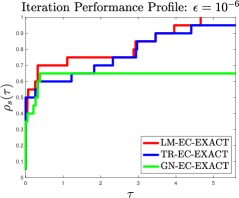
(a) Exact implementation.

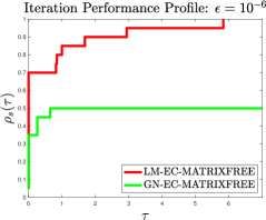
(b) Matrix-free implementation.

Figure 1: Iteration performance profiles using $20$ standard constrained least-squares problems [17].

4.3 A data assimilation problem solved using exact linear algebra

Data assimilation is of a hidden random temporal process $(X_{i})_{i=0}^{T}$, where $X_{i}$ is the state of the process at time $i$ and $T$ denotes a time horizon. This usually combines prior information about the process a numerical model and some observations. More formally, one aims to determine $x_{0},\ldots,x_{T}$, where $x_{i}\in\mathbb{R}^{n}$ is an estimator of the state $X_{i}$, from (i), the prior state $X_{0}=x_{b}+W_{b}$, $W_{b}\sim N(0,B)$, (ii) the numerical model $X_{i}=\mathcal{M}_{i}(X_{i-1})$, $i=1,\ldots,T$, where $\mathcal{M}_{i}$ is the model operator at time $i$ and (iii) the observations $y_{i}=\mathcal{H}_{i}(X_{i})+V_{i}$, $V_{i}\sim N(0,R_{i})$, $i=0,\ldots,T$. Here $T$ denotes the time horizon for the assimilation. The random vectors $W_{b}$ and $V_{i}$ represent the noise on the prior and the observation at time $i$, respectively, and are supposed to be Gaussian distributed with mean zero and covariance matrices $B$ and $R_{i}$, respectively.

The 4DVAR “strong constraint” method [2] is one of the most important data assimilation techniques for weather forecasting, that consists in computing $x_{0},\ldots,x_{T}$ by solving the following optimization problem:

(26) $$\begin{array}[]{rl}\displaystyle\min_{(x_{0},\ldots,x_{T})\in\mathbb{R}^{n(T+1)}}&f([x_{0},\ldots,x_{T}]):=\frac{1}{2}\left(\|x_{0}-x_{b}\|^{2}_{B^{-1}}+\sum_{i=0}^{T}\|y_{i}-\mathcal{H}_{i}(x_{i})\|^{2}_{R_{i}^{-1}}\right)\\ \mbox{s. t.}&x_{i}-\mathcal{M}_{i}(x_{i-1})=0,\quad i=0,\ldots,T\end{array}$$

where $x_{-1}=x_{b}$, $x=(x_{0},\ldots,x_{T})$, and $\|z\|^{2}_{M}=z^{\top}Mz$ is the norm defined by a positive definite matrix $M$. This problem conforms to our generic formulation (1). In our experiments, the numerical model is chosen to be the nonlinear Lorenz 63 system [18]: for a given $x_{i-1}=[x_{i-1}^{(1)},x_{i-1}^{(2)},x_{i-1}^{(3)}]^{\top}\in\mathbb{R}^{3}$ (i.e., $n=3$), the model is given by

$$\mathcal{M}_{i}(x_{i-1})=\begin{pmatrix}-\sigma(x_{i-1}^{(1)}-x_{i-1}^{(2)}\\ \rho x_{i-1}^{(1)}-x_{i-1}^{(2)}-x_{i-1}^{(1)}x_{i-1}^{(2)}\\ x_{i-1}^{(1)}x_{i-1}^{(2)}-\beta x_{i-1}^{(3)}\end{pmatrix},$$

where $\sigma$, $\rho$, and $\beta$ are parameters whose values are chosen as $10$, $28$, and $8/3$, respectively. These values are known to result in chaotic behavior of the Lorenz 63 model with two regimes [18]. We choose the matrices $B$ and $R_{i},\,i=0,\ldots,T$ to be identity matrices. The observations $\{y_{i}\}_{i=\{0,\dots,T\}}$ and $x_{b}$ are generated randomly. Each variable is observed through the nonlinear operator

$$\mathcal{H}_{i}(x_{i})=\frac{x_{i}}{2}\left(1+\frac{|x_{i}|^{\gamma^{\mbox{obs}}-1}}{10}\right),\quad i=0,\ldots,T,$$

where $|x_{i}|$ is the component wise absolute value of $x_{i}$ and $\gamma^{\mbox{obs}}$ is a scalar which tunes the nonlinearity of the observation operator [2, Chapter 6]. Note that the problem is smooth if $\gamma^{\mbox{obs}}$ is an odd integer.

Table 1: Results on the data assimilation problem (26) using two different $\gamma^{\mbox{obs}}$ values.

	$T$	$\gamma^{\mbox{obs}}=3$				$\gamma^{\mbox{obs}}=5$
		#it	$f(x_{j})$	$\|C_{j}\|$	$\|\hat{g}_{j}\|$	#it	$f(x_{j})$	$\|C_{j}\|$	$\|\hat{g}_{j}\|$
LM-EC-EXACT	2	83	5.9e+00	3.7e-10	8.0e-05	98	6.7e+00	7.7e-10	8.6e-05
	3	$10^{3}$	8.8e+00	1.7e-05	1.3e-01	$10^{3}$	8.7e+00	5.8e-05	1.6e-01
	15	70	2.6e+01	2.4e-09	4.5e-05	40	2.7e+01	2.7e-09	4.2e-05
	45	36	6.7e+01	2.1e-11	8.5e-05	48	6.8e+01	1.8e-09	7.7e-05
	225	58	3.4e+02	5.0e-09	6.9e-05	45	3.4e+02	1.3e-11	8.3e-05
TR-EC-EXACT	2	$10^{3}$	5.9e+00	6.1e-09	1.2e-02	$10^{3}$	6.6e+00	3.6e-08	1.5e-02
	3	$10^{3}$	7.9e+00	2.3e-16	1.0e-01	$10^{3}$	8.3e+00	2.4e-05	2.0e-01
	15	$10^{3}$	2.6e+01	9.1e-06	7.0e-02	$10^{3}$	2.7e+01	1.8e-06	2.3e-02
	45	73	6.7e+01	5.7e-09	7.6e-05	$10^{3}$	6.8e+01	1.1e-16	2.8e-02
	225	$10^{3}$	3.4e+02	6.7e-16	5.8e-03	$10^{3}$	3.4e+02	2.2e-07	5.5e-02
GN-EC-EXACT	2	$10^{3}$	3.2e+01	1.2e-01	1.0e+01	$10^{3}$	9.2e+00	2.4e-01	4.2e+0
	3	$10^{3}$	9.7e+00	3.2e-02	2.5e-01	$10^{3}$	9.2e+00	6.7e-02	9.0e-01
	15	$10^{3}$	9.7e+01	2.0e-01	2.7e+01	$10^{3}$	3.5e+02	3.0e-01	2.1e+2
	45	$10^{3}$	7.4e+01	1.2e-01	4.7e+00	$10^{3}$	1.9e+02	4.1e-02	7.6e+1
	225	$10^{3}$	3.5e+02	1.1e-01	5.3e+00	$10^{3}$	3.5e+02	2.7e-02	4.7e+0

Figure 2: Data assimilation convergence plots, considering $T=45$ and $\gamma^{\mbox{obs}}=3$.

As in the previous section, we tested our three solvers on this problem with the convergence criterion $\max(\|C_{j}\|,\|\widetilde{W}_{j}(g_{j})\|)\leq 10^{-4}$ and a maximum of $j_{\max}:=1000$ iterations. Table 1 and Figure 2 depict the performance of the algorithms in terms of the constraint and the projected gradient norms. Considering that $T=45$ and $\gamma^{\mbox{obs}}=3$, from Figure 2, we see that LM-EC-EXACT exhibits better performance compared to TR-EC-EXACT and GN-EC-EXACT: the latter method even diverges, as the values of the gradient and the constraint norm oscillate or stagnate over the iterations. On the contrary, our algorithm LM-EC-EXACT and the trust-region method TR-EC-EXACT are able to decrease both the gradient and the constraint norm to a small accuracy, with our method converging faster. Table 1 confirms the superiority of our approach on this problem: GN-EC-EXACT diverges for all instances, TR-EC-EXACT shows slightly better results as it converges for some instances, and LM-EC-EXACT converges for most of the instances.

4.4 A PDE-constrained optimization problem

We now study a least-squares problem with a hyperbolic forward PDE as equality constraints [10]. Given a time interval $[0,T]$, a time dependent density field $y(x,t)$, and a time velocity field $u(x,t)$, one wishes to solve the constrained nonlinear least-squares problem

(27) $$\begin{array}[]{rl}\displaystyle\min_{(y,u)}&f([y,u]):=\frac{1}{2}\|Qy-z\|^{2}+\frac{1}{2}\int_{\Omega}\left((u-u_{r})^{2}+|\nabla(u-u_{r})|^{2}\right)\\ \mbox{s. t.}&y+\nabla\cdot(yu)=0\\ &y(0,x)=y_{0}.\end{array}$$

where $u_{r}$ is a chosen reference model. Given the forward problem on $y$, the operator $Q$ represents the projection of $y$ onto the space of the data $z$. Since problem (27) is infinite-dimensional, we considered a discretization grid such that $d=4096$. To this end, we adapted the existing Matlab implementation of this problem available online. To initialize the variables in each optimization procedure, we used the reference model for $u$ and zero for $y$. Due to the nature of the PDE problem, only matrix-free optimization solvers can be used, hence only LM-EC-MATRIXFREE and GN-EC-MATRIXFREE were tested on this problem.

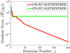
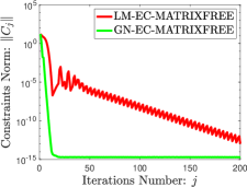
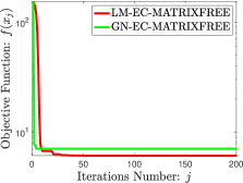
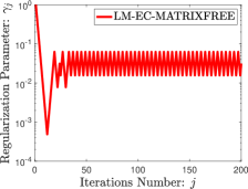
Figure 3: Convergence plots for the PDE-constrained optimization problem using matrix-free solvers.

4.5 A coupled ODE-PDE nonlinear inverse problem

We finally compare our methods on the G_Water problem described by Schittkowski [24, Section 6.3]. This inverse problem features a nonlinear least-squares objective and nonlinear constraints formed by a discretized coupled ODE-PDE system modeling acidification of groundwater pollution. The resulting infinite-dimensional optimization problem is:

$$\left\{\begin{array}[]{lrll}\min\limits_{c_{m},c_{im}}&f([c_{m},c_{im}]):=&\frac{1}{2}\left\|c_{m}(40,t)-\frac{D_{m}}{V_{m}}\frac{\partial c_{m}}{\partial x}(40,t)-\hat{h}\right\|^{2}&\\ \text{subject to}&\theta_{m}\frac{\partial c_{m}}{\partial t}(x,t)&=\theta_{m}D_{m}\frac{\partial^{2}c_{m}}{\partial x^{2}}(x,t)-\theta_{m}V_{m}\frac{\partial c_{m}}{\partial x}(x,t)&\\ &\theta_{im}\frac{\partial c_{im}}{\partial t}(x,t)&=\alpha(c_{m}(x,t)-c_{im}(x,t))&\\ &c_{m}(0,t)-\frac{D_{m}}{V_{m}}\frac{\partial c_{m}}{\partial x}(0,t)&=\left\{\begin{array}[]{ll}5800,&\text{if }t<0.01042\\ 0,&\text{otherwise}\end{array}\right.&\\ &c_{m}(80,t)+\frac{D_{m}}{V_{m}}\frac{\partial c_{m}}{\partial x}(80,t)&=0,&\end{array}\right.$$

where $\{\theta_{m},\theta_{im},V_{m},\alpha,D_{m}\}$ are parameters, $c_{m}$ and $c_{im}$ are the functions to determine, $\hat{h}$ is the infinite-dimensional observation vector, and $\Omega\times T=(0,80)\times(0,2.55]$ is the domain. The initial conditions are that $c_{im}(x,0)=0$ and $c_{m}(x,0)=0$.

In order to generate the measurements, we took the values of the parameters corresponding to the lowest residual in the reported results in [24], and simulated the PDE using a spatial discretization with $n_{x}=16$ using the ode15s MATLAB function, which generated a time discretization of $n_{t}=197$. Since there is an observation at each time point, we obtained a residual vector (corresponding to $F(x)$ in (1)) of length $197$. We used the measurements of $\tilde{h}(c_{m}):=c_{m}(40,t)-\frac{D_{m}}{V_{m}}\frac{\partial c_{m}}{\partial x}(40,t)$ at each of the time points to compute the vector of $\hat{h}$. Ultimately, the dimension of the constraints vector $C(x)$ is $m=6304$ and the number of the unknown variables was $d=6309$.

We emphasize that this problem is highly nonlinear and difficult to solve, especially with a low-quality starting point. Since we did not find recommendations for starting points in the literature, we ran our two matrix-free solvers from 150 starting points chosen uniformly at random: the final residual for $\|C(x)\|+\|\tilde{W}g\|$ was less than $10$ for 23 of the runs, while the final feasibility measure $\|C(x)\|$ was less than $10^{-1}$ on 67 of the runs. The initial values of $\|C(x)\|+\|\tilde{W}g\|$ were typically of the order of $[10^{4},10^{6}]$, which illustrates the challenges posed by this problem. Figure 4 plots the progress along the iterations of both algorithms with the lowest final value of $\|C(x)\|+\|\tilde{W}g\|$. Note that the norm of the constraint quickly drops to tolerance, which indicates that our methods produce iterates that end to respect the physics of the problem.

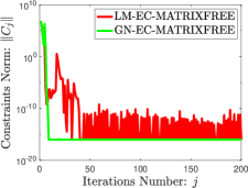
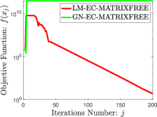
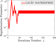
Figure 4: Performance for the first $100$ iterations on the inverse coupled PDE-ODE problem.

5 Conclusion

We have proposed and analyzed a nonmonotone composite-step Levenberg-Marquardt algorithm for the solution of equality-constrained least-squares problems. Our approach allows for approximate solutions of the subproblems computed by iterative linear algebra, and is endowed with global convergence guarantees through a nonmonotone step acceptance rule. Our numerical experiments showed that our method is competitive with trust-region approaches, and converges on a variety of experiments from data assimilation to PDE-constrained optimization.

Our theoretical analysis focuses on global convergence, yet complexity results have become increasingly popular in the optimization community. Deriving worst-case bounds on the number of Hessian-vector products required to reach an approximate solution of the problem is a potential follow-up of this work. Besides, our applications of interest such as data assimilation and PDE-constrained optimization, the measurements (and sometimes the models themselves) can be noisy, which significantly hardens the optimization task. Incorporating uncertainty into our framework thus represents an interesting avenue for future research.

References

- [1] H. Antil, D. P. Kouri, M.-D. Lacasse, and D. Ridzal, editors. Frontiers in PDE-Constrained Optimization, volume 163 of The IMA Volumes in Mathematics and its Applications. Springer, New York, NY, USA, 2016.
- [2] M. Asch, M. Bocquet, and M. Nodet. Data Assimilation: Methods, Algorithms, and Applications. SIAM, 2016.
- [3] R. Behling and A. Fischer. A unified local convergence analysis of inexact constrained Levenberg-Marquardt methods. Optim. Lett., 6:927–940, 2012.
- [4] E. Bergou, Y. Diouane, and V. Kungurtsev. Convergence and complexity analysis of a Levenberg-Marquardt algorithm for inverse problems. J. Optim. Theory Appl., 185:927–944, 2020.
- [5] E. Bergou, S. Gratton, and L. N. Vicente. Levenberg-Marquardt methods based on probabilistic gradient models and inexact subproblem solution, with application to data assimilation. SIAM/ASA J. Uncertain. Quantif., 4:924–951, 2016.
- [6] S. Boyd and L. Vandenberghe. Introduction to Applied Linear Algebra - Vectors, Matrices and Least Squares. Cambridge University Press, Cambridge, United Kingdom, 2018.
- [7] S.-C. T. Choi, C. C. Paige, and M. A. Saunders. MINRES-QLP: A Krylov subspace method for indefinite or singular symmetric systems. SIAM J. Sci. Comput., 33:1810–1836, 2011.
- [8] J. E. Dennis, M. El-Alem, and M. C. Maciel. A global convergence theory for general trust-region-based algorithms for equality constrained optimization. SIAM J. Optim., 7:177–207, 1997.
- [9] Elizabeth D Dolan and Jorge J Moré. Benchmarking optimization software with performance profiles. Mathematical Programming, 91(2):201–213, 2002.
- [10] E. Haber and L. Hanson. Model problems in pde-constrained optimization. Technical report, 2007.
- [11] P. C. Hansen, V. Pereyra, and G. Scherer. Least Squares Data Fitting with Applications. Johns Hopkins University Press, Baltimore, MD, USA, 2012.
- [12] M. Heinkenschloss and D. Ridzal. A matrix-free trust-region sqp method for equality constrained optimization. SIAM J. Optim., 24(3):1507–1541, 2014.
- [13] M. Heinkenschloss and L. N. Vicente. Analysis of inexact trust-region sqp algorithms. SIAM J. Optim., 12(2):283–302, 2002.
- [14] W. Hock and K. Schittkowski. Test examples for nonlinear programming codes. J. Optim. Theory Appl., 30:127–129, 1980.
- [15] A. F. Izmailov, M. V. Solodov, and E. Uskov. A globally convergent Levenberg–Marquardt method for equality-constrained optimization. Comput. Optim. Appl., 72(1):215–239, 2019.
- [16] K. Levenberg. A method for the solution of certain problems in least squares. Quart. Appl. Math., 2:164–168, 1944.
- [17] Z. F. Li, M. R. Osborne, and T. Prvan. Adaptive algorithm for constrained least-squares problems. J. Optim. Theory Appl., 114:423–441, 2002.
- [18] E. N. Lorenz. Deterministic non periodic flow. J. Atmos. Sci, 20(2):130–141, 1963.
- [19] D. Marquardt. An algorithm for least-squares estimation of nonlinear parameters. SIAM J. Appl. Math., 11:431–441, 1963.
- [20] N. Marumo, T. Okuno, and A. Takeda. Constrained Levenberg-Marquardt method with global complexity bound. arXiv:2004.08259, 2020.
- [21] J. Nocedal and S. J. Wright. Numerical Optimization. Springer Series in Operations Research and Financial Engineering. Springer-Verlag, New York, second edition, 2006.
- [22] D. Orban and A. S. Siqueira. A regularization method for constrained nonlinear least squares. Comput. Optim. Appl., 76:961–989, 2020.
- [23] K. Schittkowski, editor. More Test Examples for Nonlinear Programming Codes. Springer-Verlag, Berlin, Heidelberg, 1987.
- [24] K. Schittkowski. Parameter estimation in one-dimensional time-dependent partial differential equations. Optim. Methods Softw., 7(3-4):165–210, 1997.
- [25] T. Steihaug. The conjugate gradient method and trust regions in large scale optimization. SIAM J. Numer. Anal., 20:626–637, 1983.
- [26] A. Tarantola. Inverse Problem Theory and Methods for Model Parameter Estimation. SIAM, Philadelphia, 2005.
- [27] Y. Trémolet. Model-error estimation in 4D-Var. Quarterly Journal of the Royal Meteorological Society, 133:1267–1280, 2007.
- [28] M. Ulbrich and S. Ulbrich. Nonmonotone trust region methods for nonlinear equality constrained optimization without a penalty function. Math. Program., 95:103–135, 2003.