A Generative Neural Network Framework for Automated Software Testing

Abstract.

Search Based Software Testing (SBST) is a popular automated testing technique which uses a feedback mechanism to search for faults in software. Despite its popularity, it has fundamental challenges related to the design, construction and interpretation of the feedback. Neural Networks (NN) have been hugely popular in recent years for a wide range of tasks. We believe that they can address many of the issues inherent to common SBST approaches. Unfortunately, NNs require large and representative training datasets.

In this work we present an SBST framework based on a deconvolutional generative neural network. Not only does it retain the beneficial qualities that make NNs appropriate for SBST tasks, it also produces its own training data which circumvents the problem of acquiring a training dataset that limits the use of NNs.

We demonstrate through a series of experiments that this architecture is possible and practical. It generates diverse, sensible program inputs, while exploring the space of program behaviours. It also creates a meaningful ordering over program behaviours and is able to find crashing executions. This is all done without any prior knowledge of the program.

We believe this proof of concept opens new directions for future work at the intersection of SBST and neural networks.

1. Introduction

In this paper we explore an automated testing framework based on Neural Networks (NN). The proposed approach aims to address some of the most pertinent problems of both automated testing and generative NN models. This proof of concept introduces multiple new ideas at the intersection of automated software testing and generative neural networks, and we hope it will stimulate further research in this area.

Automated testing techniques have become increasingly popular thanks to the availability of resources and their ever improving effectiveness. We view automated testing from the perspective of Search Based Software Testing (SBST) (Harman and Jones, 2001; McMinn, 2004). In SBST, a program is repeatedly executed, its execution monitored and further executions are generated with the aim of more effective fault discovery. Commonly the goal is to optimise coverage. A fundamental feature of SBST is the reliance on a feedback mechanism to evaluate and direct the search.

The practical instantiation of SBST that we consider is fuzzing. Fuzzing is a technique where a program is bombarded with random inputs in hopes it will eventually crash (Sutton et al., 2007). Modern fuzzers however use feedback mechanisms to improve their effectiveness. Using a feedback loop for improving search brings fuzzing into the realm of SBST. A popular modern fuzzer is the American Fuzzy Lop (AFL) (Zalewski, 2007). Although it does use a feedback mechanism and hence falls into the realm of SBST, its search strategies and notions of similarity are non-principled heuristics – they ”just work”. That said, these heuristics all ultimately drive the fuzzer towards exploring a program’s behaviours maximally diversely. Indeed, diversification is generally a very common target for testing (Ammann and Offutt, 2016; Heimdahl et al., 2004; Gay et al., 2015); after all, if the target of search is unknown, the best you can do is explore.

Although popular both in academia and industry, SBST is not without its limitations (McMinn, 2011; Aleti et al., 2017). The problems of SBST we aim to address are the following. First, fitness landscapes of SBST may have plateaus or be discontinuous. Then either multiple adjacent candidate solutions appear equivalent in terms of fitness and the search mechanism cannot prioritise them or it cannot move to a better solution. Second, the fitness landscape may contain local optima which leads the search to a sub-optimal solution. Third, choosing the representation requires domain knowledge and expert involvement (Shepperd, 1995). Fourth, it is not apparent how to assign an ordering onto the search landscape, likewise requiring an involvement of an expert (Shepperd, 1995; Harman and Clark, 2004). Granted, it can be defined in terms of the search operators, i.e. candidate solutions one search step away from each other are adjacent. But is this the best ordering for the search? Finally, the generation of new candidate solutions is a big can of worms with various approaches and solutions (McMinn, 2004; Anand et al., 2013; Ali et al., 2010; Alshraideh and Bottaci, 2006; Fraser and Arcuri, 2013, 2011; Fraser and Zeller, 2012; Pacheco and Ernst, 2005; Korel, 1992). What search operators to use? How much prior knowledge is required and available? How to produce the next candidate solution?

We propose that NNs’ properties make them ideal for tackling these issues. First, NNs are trained by a process of backpropagation (Rumelhart et al., 1986) which means they must be differentiable and thus continuous by construction (Glasmachers, 2017). That is, if a neural network trains, its intermediate states must be differentiable. This continuity and differentiability make NNs a natural candidate to tackle the issue of plateaus in SBST search spaces. Second, it has been shown that given sufficient size, NNs avoid local optima (Kawaguchi, 2016; Swirszcz et al., 2016; Nguyen and Hein, 2017, 2018). Third, the above property also implies that if a representation contains a useful signal, an NN will discover it. This means that they can use representations that are difficult to interpret manually. NNs may suffer from noise given redundant data, but these problems can be addressed with feature selection (Verikas and Bacauskiene, 2002; Leray and Gallinari, 1999; Wang et al., 2014) and modern, deep architectures suffer less from this problem (Li et al., 2018). This alternative is nonetheless preferable to a major manual effort. Fourth, due to their differentiable nature, NNs impose an order relation onto data (e.g. (Kingma and Welling, 2013)). They may thus help us reason about similarity and diversity of program behaviour in a principled, continuous way. Lastly, NNs can be used for generating new data without analytical human effort (Goodfellow et al., 2016; Kawthekar et al., [n.d.]; Chollet, 2017; Graves, 2013; OpenAI, 2016; Radford et al., 2015; Van Den Oord et al., 2016).

NNs, as tools for SBST, come with limitations of their own however. The main problem is that they are data hungry; they need large representative training datasets (Beleites et al., 2013). This appears like a disqualifying issue in the context of SBST. If one wishes to train an NN to be used as a fuzzer, and has sufficient data to train the NN, this data could simply be used to test the program itself. This really defeats the purpose of building and training an NN-based fuzzer.

The architecture proposed in this work can address all these problems – SBST and NN related alike. It is a generative model that produces its own training data. In a way, this architecture is similar to that of reinforcement learning (RL) where an agent explores an environment, discovers rewards and learns to navigate the space more effectively. In our approach, the agent is the generative model while the program under test is the environment. This might seem like a bizarre proposition as there is no apparent way to evaluate the quality of the generated data. You can produce all the random data you like, but how do you know if it is any good? What is your reward signal? We suggest that the principle of diversification can be adapted from SBST to evaluate the generated data; the model is rewarded for diversity.

This framework we call GNAST (Generative Network for Automated Software Testing) begins by throwing random inputs at a program. Most of these will be rejected by the program. Some, however, will trigger an unusual execution trace. Those are prioritised and kept in the training dataset. As the process continues, GNAST generates program inputs that trigger new behaviours and uses them in its training dataset. The fact that GNAST is NN based allows it to address the issues outlined above, as we will show in the sequel.

In this work we implement a prototype of GNAST and present a number of initial findings. First and foremost, we show how such a system can be trained and how it produces diverse program inputs. Furthermore, the inputs are clearly sensible with respect to the syntax of the program under test. In addition, we can control the syntactic similarity of generated strings. Finally, rudimentary as the current state of GNAST is, it does actually discover crashes. Currently it is a prototypical proof of concept accompanied by several outstanding questions. As such, it cannot be readily compared with fully fledged fuzzers like AFL.

Even though it is a prototype, GNAST presents a number of novel ideas. It is a generative NN-based automated software testing tool that does not require a training dataset – it produces its own. It is a new example of a deconvolutional generative model for string generation. It uses a novel quantified notion of similarity for program executions. It presents a prioritisation method for program executions based on a greedy algorithm called Farthest-First Traversal (FFT). Finally, it uses ”unusualness” and diversity as an explicit training target and although this idea is common in testing, it is novel in this formulation.

2. Overview of Approach

We propose a framework for automated software testing. Its purpose is to explore the behaviours of a Software Under Test (SUT) diversely. Our system does this by generating inputs for the SUT, observing the executions under those inputs and adjusting further generation of inputs towards the most unusual behaviours. It is essentially an evolutionary fuzzer, albeit with convoluted generative and feedback mechanisms.

The tool is based on two neural networks (NN), an execution trace profiler and a prioritisation mechanism of executions. The structure is shown in Figure 1 and its algorithm is presented in Algorithm 1. A single epoch of the algorithm corresponds to two passes through the framework in Figure 1: the first is a generative pass where the networks’ weights are not updated, and a training pass – where they are. The algorithm and framework are described next, with the numbers in brackets corresponding to the lines in Figure 1 and Algorithm 1.

The process is initialised by feeding Gaussian noise to an untrained Generative Neural Network (GNN) (2-6). It produces a batch of program inputs $X$. Most of these will be nonsensical; strings of random characters. The inputs are then executed by the SUT and the execution traces $T$ are collected (12). As most inputs are just noise, most execution traces will yield the ”invalid input” execution trace. Some inputs however may contain features that are valid, which will be reflected in their execution traces.

The execution traces are then encoded by a Variational Autoencoder (VAE) (14). It casts the discrete, unorderable execution trace into an n-dimensional ”latent” space encoding $E$. The latent space encoding is a quantifiable representation of features of execution traces, and we can reason about their similarity in terms of Euclidean distance. The encoded executions are then ranked by the ”unusualness” of their encoded traces using the Farthest-First Traversal (FFT) algorithm (18). Redundant datapoints are discarded and the most interesting ones are kept in a persistent training dataset (20). The dataset is composed of the execution traces $T$, their encodings $E$ and the program inputs that triggered them $X$.

The dataset is then used to train both the VAE and the GNN (24, 26). As the VAE learns to encode the execution traces of the training dataset, new, unusual ones stand out from the bunch. The GNN, in turn, learns to produce program inputs that trigger a variety of traces, i.e. program behaviours. We also add noise to perturb the dataset towards exploration so that more novel behaviours are found (29). We suggest that the proposed framework represents a fundamentally novel approach to using neural networks for diversity driven testing of programs.

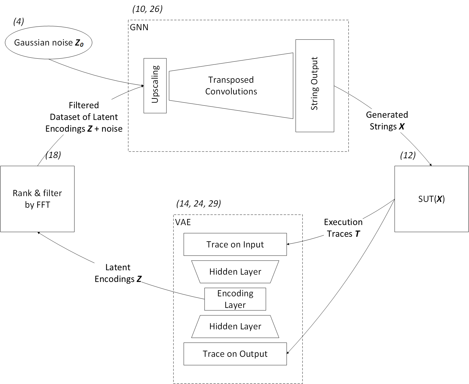
Figure 1. The GNAST Framework. A detailed explanation of the training and generative processes is given in Section 2. The algorithm corresponding to this image is shown in Algorithm 1, with numbers in brackets corresponding to line numbers.

1// Initialise epoch counter

2 $e\leftarrow 0$;

3 // Initialise inputs to GNN from Gaussian noise

4 $\{Z_{0}\}\sim\mathcal{N}(\mu,\,\sigma^{2})$;

5

6// Initialise dataset of program inputs, traces and GNN inputs

7 $\{Res_{0}\}\leftarrow\{<X=\emptyset,T=\emptyset,Z=Z_{0}\}$ ;

8

9while $\top$ do

10      

11      begin Generative pass

12             // Generate a batch of program inputs

13             $\{X_{e}\}\leftarrow GNN(Z_{e})$;

14             // Execute SUT, collect traces

15             $\{T_{e}\}\leftarrow SUT(X_{e})$;

16             // Get encodings of traces

17             $\{Z_{e}\}\leftarrow VAE_{train=\bot}(T_{e})$;

18            

19            // Append new inputs, traces and strings to the dataset

20             $\{Res_{e-1}\}\cup\{<X_{e},T_{e},Z_{e}>\}$

21            // Rank traces with FFT

22             $R_{e}\leftarrow FFT(T_{e})$;

23             // Discard redundant datapoints, limit of k=5000 due to hardware resource limitation

24             $\{Res|r_{i}<k\}$;

25            

26       end

27      

28      begin Training pass

29             // Train VAE on representative traces

30             $VAE(T_{e})_{train=\top}$;

31             // Train GNN on representative noises and inputs

32             $GNN(<X_{e},Z_{e}>)_{train=\top}$;

33            

34       end

35      

36      // Update the inputs with encodings of traces

37       $\{Z_{e}\}\leftarrow VAE(T_{e})_{train=\bot}+\epsilon\sim\mathcal{N}(\mu,\,\sigma^{2})$;

38       // Increment epoch

39       $e\leftarrow e+1$;

40      

41 end while

42

Algorithm 1 The algorithm for training and generating inputs with GNAST. The algorithm corresponds to the image in Figure 1 and described in Section 2.

3. Research Questions

While many of the individual mechanisms of GNAST are inspired by other work, the overall structure is fundamentally novel. It is an RL-inspired loop that generates training data for itself by sampling the output distribution and evaluates samples with an external diversity-driven oracle. The novelty brings about a huge number of design and configuration decisions, all of which have an effect on the research questions outlined below.

First, there was no guarantee that the training of such a system would converge at all. It is also not clear what optimisers, layer sizes, numbers of hidden layers etc. to use. Non-convergence is essentially underfitting – the mechanism does not learn to approximate the data. Whether GNAST’s training converges is the the focus of the first research question.
RQ1: ”Does GNAST framework’s training converge?”

Second, it is insufficient for GNAST’s training to simply converge. It also needs to not converge too far, so as to continue generating new datapoints. New datapoints are essential both for exercising varied behaviours of the SUT as well as building up a diverse dataset for training. Much like non-convergence in RQ1 means underfitting, converging too far corresponds to overfitting – the system learns to produce only a few datapoints and since those are kept in the training dataset, their effect becomes ever stronger. The second research question looks at diversity during training.
RQ2: ”Does GNAST maintain diversity throughout training?”

Third, if the mechanism does train in an acceptable way, we then need to evaluate whether the produced program inputs are sensible. Granted, a program may crash under a completely unexpected random input, but a fundamental principle of fuzzing (and indeed any other testing) is that inputs ought to be consumable by the SUT, beyond an ”invalid input” check. This means they ought to be somewhat well-formed, or at least have some relevant syntactic features. AFL generates strings that can hardly be called well-formed, as the representation yielded by its instrumentation is only a crude representation of a program’s behaviour. Since the instrumentation is lifted out of AFL, the strings generated by GNAST were expected to contain some syntactic feature similar to those made by AFL, but there was no expectation of the them being properly well-formed. The aim of the third research question is to see whether the generated strings are completely random or comparable in structure to those made by AFL.
RQ3: ”Do the generated program inputs have syntactic features similar to those generated by an AFL baseline?”

Fourth, one of the intended features of GNAST is the ability to control the similarity of syntactic features of the produced inputs by adjusting the input. Once GNAST is trained, the latent space that was used as input to the GNN can be replaced with n-dimensional normal noise. The GNN thus becomes a stand-alone generator which takes a vector of reals as input and generates a string on the output. Input values close to each other are ought to produce similar strings while distant inputs should produce dissimilar ones. Whether this is the case is investigated in the fourth research question.
RQ4: ”Do strings generated from nearby points in the latent space share syntactic features vs. those far apart?”

Fifth, by the same design as syntactic similarity of generated program inputs, GNAST ought to be able to generate strings that would trigger a specific desired behaviour. After all, one of the components of the loss function is the reconstruction of input. Our fifth research question looks at this aspect.
RQ5: ”Can GNAST generate input strings that trigger specific behaviours of a SUT?”

Finally, although GNAST is only a proof of concept with a lot of additional work to be done, we would like to know if the framework ”has legs” as a design for a fuzzer. The ultimate aim of a fuzzer is to find crashes, and our last research question is simple but poignant.
RQ6: ”Does GNAST discover crashes in sparse?

4. Related Work and Background

The proposed framework applies machine learning techniques, specifically GNNs, to automated software testing. This section links the mechanisms of GNAST to concepts, ideas and inspirations in those fields.

4.1. Fuzzing and the American Fuzzy Lop

Fuzzing is an automated testing technique which attempts to discover faults by bombarding a program random inputs (Sutton et al., 2007). Modern fuzzers use feedback to improve the input generation process; they evaluate their progress in order to search for faults more effectively.

American Fuzzy Lop (AFL) is a popular fuzzer widely used in academia (Zalewski, 2007). A number of recent papers have taken AFL as a basis, and improved on it. These include work on improving AFL’s instrumentation (Gan et al., 2018; Chen and Chen, 2018), alternative search strategies (Böhme et al., 2017a; Böhme et al., 2017b; Petsios et al., 2017), producing better initial seeds (Lv et al., 2018), locating interesting input string mutation locations (Rajpal et al., 2017; She et al., 2018) and introducing program context information (Rawat et al., 2017). Although we use some parts of AFL, our work does not attempt to improve AFL. Instead, we are proposing a fundamentally different architecture.

4.2. Representation and Fitness Function

Feedback-driven automatic testing tools like modern fuzzers, fall under the field of Search Based Software Testing (SBST) (Harman et al., 2012; McMinn, 2004). As any other SBST approach, the design of a fuzzer depends on a representation and a fitness function (Harman and Jones, 2001).

Representation is the choice of what to observe about a candidate solution, in this case an execution. It may be a coverage profile, a sequence of executed basic blocks or something simple like execution time. In this work, the representation is based on the execution trace profiling mechanism from AFL. AFL’s representation of an execution is an approximate count of decision point transitions. It does not capture context nor sequence information about the execution.

The fitness function is what transforms a representation into a quantified assessment of quality of a candidate solution. But what constitutes quality in fuzzing and how can it be quantified?

Fuzzing, and software testing in general, aims to exercise program behaviours diversely: diversity is quality. The original AFL uses a handful of heuristics to identify executions that are distinct or ”interesting”, i.e. of high quality. For instance, if an execution exercises a transition that has not been previously seen, it is considered interesting. Whilst the heuristics of AFL are empirically effective, they are not principled and do not order nor quantify the similarity of executions or behaviours.

4.3. Quantifying Program Behaviour

GNAST is intended to give an ordering, and quantify the similarity of executions. The approach relies on an autoencoder neural network which is used to process execution traces. An autoencoder is an NN which attempts to reconstruct its inputs at the outputs, while arranging the datapoints into an n-dimensional encoding (”latent”) space by similarity of their features (Goodfellow et al., 2016). Specifically, we use a flavour of an autoencoder called the Variational Autoencoder (VAE) (Kingma and Welling, 2013). The essential detail of a VAE is in the structure of its encoding layer. Rather than encoding datapoints as single real number values, they are instead encoded as tuples of mean and variance $(\mu,\sigma^{2})$. The result of this construction is that datapoints tend to be more evenly spread across the latent space and interpolation between them is smoother than in a regular autoencoder.

In GNAST, the inputs and outputs to the VAE are the execution traces and the latent space encoding is a representation of their most salient (i.e. most distinguishing) features. The benefit of encoding traces in this way is that it imposes an order relation on discrete, seemingly unorderable datapoints. Furthermore, the space is continuous and smooth. These are characteristics of a good search landscape (Harman and Clark, 2004). Since execution traces are the representation of program behaviour, the latent space in fact constitutes the space of behaviours. We suggest that since we want to explore diverse behaviours, this latent space is what we ought to be exploring diversely.

4.4. Ranking Algorithm

Once we have constructed an n-dimensional Euclidean space to represent program behaviours, we need a method for evaluating which datapoint is unusual and which is redundant. We propose doing this using an algorithm known as the Farthest-First Traversal (FFT) or the greedy permutation. FFT arranges a set of points into a sequence such that the minimal distance of each following point is maximised. In other words, the prefix of the sequence is always maximally representative of the whole dataset. We are not aware of work which would use FFT in ranking candidate solutions in SBST.

The algorithm is shown in Algorithm 2 and described below, with line numbers shown in brackets. Prior to the actual algorithm, the pairwise distance of each datapoint is calculated (2). Then the result is initialised with two maximally distant elements (3). The next element to append is chosen such that it is furthest from ones already in the result sequence, i.e. the minimal distance is maximised (5). Each following element in the sequence is thus maximally different from ones already in the prefix.

Once the dataset is sequenced, its tail (the most redundant portion) is discarded. We propose that pruning the dataset according to this notion of similarity keeps it diverse and maximally representative.

Data: List X of n-dimensional coordinates of elements x

Result: Result Y of tuples y of (indices, distances) $(i,d)$

1 begin

2       Calculate the pairwise distance matrix $D$;

3       Initialise Y with $y_{0},y_{1}$ of $d_{max}$;

4       while $|Y|<|X|$ do

5             Append $x$ s.t. min distance to $\forall y\in Y$ is max;

6            

7       end while

8      return $(i,d)\in Y$

9 end

10

Algorithm 2 The greedy permutation or Farthest-First Traversal (FFT) sequences elements such that each successive element maximises the minimal distance to elements in the result.

4.5. Generative Neural Networks

The heart of GNAST is a Generative Neural Network (GNN) that is trained to produce program inputs using the culled, representative dataset. As the dataset expands, the generator gets new datapoints to drive its training towards previously unseen behaviours and program inputs.

Perhaps the best known example of a GNN design for strings is the Recurrent Neural Network (RNN) (Goodfellow et al., 2016; Rumelhart et al., 1986; Hochreiter and Schmidhuber, 1997). A very early version of GNAST was implemented with an RNN (modelling on work by Bowman et al. (Bowman et al., 2015)), but it was much too slow to train and to generate new inputs, so that design was abandoned.

Our generator is therefore based on an alternative design, inspired by the Deconvolutional Generative Adversarial Network (DCGAN) (Radford et al., 2015). In DCGAN, two neural networks – a generator and a discriminator – are pitched against each other. The generator takes Gaussian noise as input, passes it through a stack of transposed convolutions (Goodfellow et al., 2016) and produces an image on the output. The discriminator takes an image as input and outputs an answer of whether the image was real or fake (generated). While the discriminator learns to be ever more effective in telling fake images from real ones, the generator attempts to produce images that fool the discriminator into believing they are real. This tandem of networks ends up creating realistic images.

There are two significant problems of readily applying DCGAN to generation of discrete data. The first problem is that unlike pixel values in images, discrete variables such as characters in strings are not readily orderable. For instance, ”bat” is not semantically almost the same as ”cat” although the two words only differ by a single (alphabetically adjacent) character: $"cat"\neq("bat"+1.0)$ (Goodfellow, [n.d.]). On the other hand, in continuous variables such as pixel hue values, a slight offset does not dramatically change the meaning: a cat can be still identified even if the image is slightly blurry.

The other problem, inherent to neural networks, is the need for a lot of training data (Beleites et al., 2013). DCGAN requires a corpus of real datapoints for training the discriminator. This in itself is a disqualifying requirement for a fuzzer, as it would require a large, representative dataset of valid program inputs. This defeats the purpose of a fuzzer: if you have a truly representative dataset of inputs, it could just be used to test the program. Furthermore, using only valid inputs would train the generator to produce only valid inputs. This is not ideal for fuzzing, as the program ought to be tested on both valid and invalid inputs.

In GNAST, in place of a discriminator network, we have the combination of a SUT, a VAE and FFT ranking. This mechanism serves the same purpose as the discriminator in DCGAN: to, as it were, quantify the quality of candidate solutions. Furthermore, thanks to the VAE, we have a continuous input space ordered by features of execution traces. This ordering of the input space imposes an order on the generated strings. In addition, we have unlimited training data thanks to GNAST producing its own. These design features thus address major problems of the use of generative models for string generation.

In the machine learning arena, the networks employed in this prototype are not novel. Recent advances in GNNs have brought about numerous novel architectures, many of them for image generation, e.g. (He et al., 2016b; Karras et al., 2019; Zhang et al., 2017), and even for text generation (Bowman et al., 2015; Wang et al., 2018). Indeed the concept of training an NN given some response from an external source is reminiscent of RL. From this point of view, the GNN represents the actor, the SUT is the environment, and the VAE with FFT is the critic(Konda and Tsitsiklis, 2000).

As for the direct use of GNNs for test input generation – the closest use case to ours – we are only aware of work by Godefroid et al. where an RNN was used to test a PDF reader (Godefroid et al., 2017) with mixed results.

5. Experimental Setup

This section presents the implementation details of each component of GNAST, as well as the experiments we ran. To the best of our knowledge, the proposed framework is novel in many aspects. A large part of our experiments was therefore exploratory; various designs and configurations were considered and tested, albeit not exhaustively due to resource limitations. The NN mechanisms were implemented with the Tensorflow framework (Abadi et al., 2015). Citations to standard deep learning concepts are omitted for clarity, and the reader is referred to the Deep Learning Book (Goodfellow et al., 2016) for reference.

5.1. Trace Profiling

Two mechanisms are lifted out of AFL: the program instrumentation (and hence representation) and the execution harness. To be clear, none of AFL’s generative or prioritisation mechanisms were used. We did not modify or parametrise these mechanisms, so there are no options to be considered, save for, of course, replacing the instrumentation with an alternative tool altogether.

AFL’s execution trace representation is a count of decision point transitions. First, the source code is instrumented with a drop-in replacement for GCC (or G++ or Clang) prior to testing. For efficiency, only a rough number of transitions is kept (8 buckets), and the trace is of a fixed size of 64K. An execution trace is thus a 64K long, typically very sparse vector with 8 distinct values. Although GNAST does not take advantage of the efficiency of this representation but it is nonetheless appropriate for three reasons. First, it is simple to implement by adapting AFL’s code. Second, the empirical evidence of AFL’s performance is in and of itself an indication of the representation’s effectiveness. Finally, there are many new aspects to our framework, and using an alternative, potentially ineffective trace representation would add to the uncertainty of the framework overall.

AFL’s execution harness is referred to as a ”fork server”. The basic idea of the fork server is to spin up the SUT up to the initial main() call and keep a snapshot of the program in that state. Whenever the SUT is executed under a new input, this initial state is copied and execution proceeds from there. Thanks to this simple mechanism, the time required for initialisation is avoided and fuzzing becomes much faster, so the inputs produced by the fuzzer can be executed quickly.

5.2. Variational Autoencoder

The VAE is composed of an encoder and a decoder, modelled on the architecture of Kingma’s work (Kingma and Welling, 2013). The encoder is as follows. The first layer is the input of size 64K, matching the size of the trace. This is followed by one or more densely connected hidden layers. Next is the encoding layer which is composed of a densely connected $\mu$ and $\sigma^{2}$ layers. In addition, the encoding layer includes a source of Gaussian noise. The construction of the encoding layer $z$ is shown in Equation 1. Once the VAE has been trained, the VAE is queried for an encoding of a trace, it is $\mu$ layer’s output that is fetched. That is, $\sigma^{2}$ and $z$ layers are only used during training to give the latent space the desired characteristics, but the actual encoding is the value $\mu$.

(1) $$z=\mu+e^{0.5\sigma^{2}}*\mathcal{N}(0,I)$$

The output of the $z$ layer is fed to hidden layer(s) of the decoder. The output of the decoder a categorical softmax layer of size $(64K,8)$. This is specific to this trace representation where counts of state transitions are bucketed into 8 values. This allows the VAE to be trained using categorical cross-entropy.

The loss function of the VAE is composed of two terms, as shown in Equation 2. The first term is the reconstruction loss and the second is the latent encoding regularisation loss. The purpose of the former is to get the VAE to actually encode the data. The latter term forces the latent space to approximate a normal distribution; to give it a convenient shape. More technically, the loss components are the Kullback-Leibler divergence between the approximate ($q$) and the true posterior ($p$) distributions, given datapoints ($x$) and model parameters ($\theta$), and the lower bound ($\mathcal{L}$)w on the marginal likelihood of datapoint i respectively (Kingma and Welling, 2013).

(2) $$loss_{VAE}=D_{KL}(q_{\phi}(z|x^{(i)})\|p_{\theta}(z|x^{(i)}))+\mathcal{L}(\theta,\phi;x^{(i)})$$

The configurable parameters of the VAE are the number, size and activation functions of hidden layers, the size and noise rate of the encoding layer as well as the losses and optimisers. These parameters affect the nature of the VAE.

We are not aware of work formally defining a ”good” VAE but from first principles of NNs, we can assume that the latent space must not be underfitted nor overfitted. Avoiding underfitting means that the VAE needs to encode the features of the data. The purpose of this is obvious: if the network does not encode the data, its latent space has no meaning whatsoever. Under visual inspection, an underfitted latent space appears like a spherical cloud of points around zero. Practically, underfitting can be easily identified by whether the model’s loss value descends – i.e. the network trains. An overfitted latent space, in turn, looks like a manifold, e.g. a line. In this case the network learned to simply memorise the datapoints and mapped them to distinct points, rather than an area. In the case of overfitting, the latent space encoding is likewise meaningless.

5.3. Generative Neural Network

The input to the GNN is the encoding of a trace produced by the VAE, with addition of small Gaussian noise $\sigma=0.1$. Gaussian noise as input was also considered but discarded as a less interpretable; there would be no mapping from behaviours to program inputs. The purpose of this noise is to perturb the data so that the framework explores novel behaviours. Much like in DCGAN, the input is then upscaled with a densely connected layer(s), and reshaped to match the size of the output of the GNN (using deconvolutions with stride $>1$). The main portion of the GNN is a stack of transposed convolutions (commonly called ”deconvolutions” – hence DCGAN) with strides one or two. This stack of deconvolutions may also include shortcuts, i.e. residual blocks (He et al., 2016a). These are intended to strengthen the signal through the network thereby alleviating the vanishing gradient problem (Hochreiter, 1998).

The output layer is of size $(str\_len_{max},dict\_size)$. In our experiments the maximum string length $str\_len_{max}$ was fixed at $512$ and the number of possible characters $dict\_size$ was 129: 128 ASCII characters and 0 for padding. During training, the output layer is trained using softmax cross-entropy of one-hot encoded strings and the reproduction error of the encoded trace (Equation 3). The first term $-\sum_{c=1}^{M}y_{o,c}\log(p_{o,c})$ trains the the GNN to approximate the mapping of trace encodings to strings. It is a standard loss for training categorical classifiers (Goodfellow et al., 2016). The second term $|\hat{z}-z|$ aims to approximate the SUTs semantics within the GNN. This term is minimised when the value of the encoded trace on the input $z$ to the GNN matches the true trace $\hat{z}$ encoding that the SUT produces when executed under the generated input. The overall loss function maps traces to strings and tries to make those strings produce a specific behaviour.

(3) $$loss_{GNN}=-\sum_{c=1}^{M}y_{o,c}\log(p_{o,c})+|\hat{z}-z|$$

During generation, rather than simply choosing the most likely character for each index of the output string (”argmax”), the generator samples from the output probability distribution, $x=\langle x_{i}\sim p_{i};i<str\_len_{max}\rangle$. This sampling technique selects plausible (rather than most likely) characters given a learned probability distribution.

There are numerous possible parameter configurations for the GNN. Common options include the size and the number of upsampling and deconvolutional layers, activation functions and optimisers. In addition, fundamental architectural options had to be considered. Namely, whether to use string reconstruction cross-entropy, trace reconstruction MSE or their combination as a loss; whether to use trace encodings or Gaussian noise as the input; and whether to sample or use argmax on the output.

5.4. Experiments Conducted

We conducted experiments on three SUTs that take strings with complicated grammar as input. The first one is an XML linter called xmllint from libxml (Veillard, 2019). The second is sparse (Jones, 2019), a lightweight parser for C (Jones, 2019). The last program is cJSON, a parser for the JSON format (Gamble, 2019). Generating inputs for these programs out of thin air is a non-trivial task. Also, since these programs validate their inputs by design, the validation process ought to be reflected in execution traces. Execution traces that depend on syntax validation would give GNAST and AFL a good representation to work with.

For the comparative analysis against a baseline, we first ran AFL on each program for 48 hours. This produced 3240, 11286 and 2071 queue inputs for xmllint, sparse and cJSON respectively. Of the three SUTs, AFL only found crashes in sparse.

In GNAST’s implementation, we evaluated its the performance under dozens (if not hundreds) of parameter configurations. There was not a fixed time budget, nor a strict performance measure for each configuration. Instead it was a trial and error exploration of the effects of various configurations with respect to the research questions. Once the most promising structure and configuration was found, we trained GNAST on each program for 48 hours. These trained instances of GNAST were then be used for RQs three through six.

6. Results

The research questions explore the nature of the proposed architecture. The findings of our investigation show that GNAST does indeed train while maintaining diversity, that it produces sensible program inputs, and that proximity in the latent space corresponds to similarity of generated strings. However, the result to RQ5 was negative: we cannot generate program inputs that would trigger specific program behaviours. Finally, GNAST does find crashes in sparse – the SUT in our corpus where AFL also found crashes.

6.1. RQ1 – Training Convergence

GNAST trained successfully under some configurations, however it failed under others. Unlike standard NNs, a successful training is not meant to converge arbitrarily close to zero because GNAST is ought to continually produce new data. Instead, the convergence ought to be simply noticeable. Our primary definition of failure is the failure to converge, i.e. underfitting. A secondary notion of failure is instability – a case when the training failed with the loss reaching inf. In fact, these two effects correspond to a vanishing and exploding gradient problems respectively (Hochreiter, 1998; Pascanu et al., 2012).

The VAE’s loss failed to converge when the noise in the encoding layer was too high and when the hidden layers were very small, e.g. 8 units. Lowering the amount of noise to $\sigma=0.1$, using 512 or more neurons in the hidden layers along with a Leaky ReLU activation allowed the VAE to converge.

GNN’s training did not converge when the structure was too weak; there were too many layers or too few filters. When it came to depth, more than a dozen layers did not appear to converge in a reasonable time. Residual blocks resolved this issue however and structures of up to 64 layers converged. With fewer than 32 filters the network also failed to converge.

Initial configurations often resulted in instability, indeed much more often than we had previously encountered in working with NNs. We believe there are three reasons for the instability. The first is aggressive optimisers, particularly Adam (Kingma and Ba, 2014). Adam is susceptible to instability when close to convergence (Wilson et al., 2017), which is a potential explanation. The second reason is Gaussian noise in the latent layer of the VAE and on the input to the GNN. Lowering the noise $\sigma$ to $0.1$ resolved this instance of instability. The last cause, we suggest, is the constantly shifting dataset. This is the most unusual reason, specific to GNAST, but not to NNs in general. Modern optimisers like RMSProp (Tieleman and Hinton, 2012) and Adam both keep track of past gradients to calculate the next optimisation steps. Adam also uses momentum. Injecting new data throws these optimisers off: taking a step towards what previously seemed an optimal point, and finding a completely unexpected datapoint there causes the loss to diverge. We are not aware of work where the training dataset would be updated like in GNAST so this suggestion is speculative, and warrants further research.

The final, most promising set of hyperparameters was the following. An RMSProp optimiser with a learning rate to $0.0001$, $42$ convolutional layers with residual connections, a kernel size of $3$, Leaky ReLu activation, batch normalisation after activation, VAE’s latent encoding as input, and a categorical cross-entropy loss.

The training loss followed an unusual trajectory: first down quickly, then up, then down slowly again. This is not a major finding per se, but an observation of expected behaviour, given a framework that produces its own training data. While there are few datapoints at the start of training, the model quickly learns how to reproduce them and the loss goes down. As new datapoints are found, the loss increases, and then slowly descends again when features of the new datapoints are learnt.

The central finding of this RQ is that GNAST trains. The positive outcome to this RQ validates the principle of GNAST and makes subsequent questions worthwhile.

6.2. RQ2 – Diversity During Training

The second property of a successful training process is that it maintains diversity. Since GNAST produces its own training data, it is critical for the framework not to collapse into generating the same outputs over and over. Overfitting was seen both in the VAE and the GNN. We consider a model failing to maintain diversity if no new traces are produced over 20 epochs of generation and training.

When the VAE was too powerful, the loss tended close to zero and under visual inspection, the latent space looked like the datapoints are placed on a manifold. This occurred when there was no noise or the hidden layers were too powerful (too many cells or layers). In this scenario, the locality in the latent space is meaningless which rids the VAE of its purpose. That is to say, an overfitting VAE is a useless structure with respect to ordering the execution traces – not necessarily an immediate problem for diversity.

Making the GNN too strong would in turn result in a reduction in diversity of generated strings. Too many filters in the deconvolutional layers, too little noise on the input or when the dropout rate was set too low – all contributed to a diminished diversity. We do not have a principled explanation for this, but it may be due to the GNN effectively learning to ignore the input layer and just encoding the dataset into its structure, before it manages to become sufficiently diverse and representative – an artefact of the recursive nature of GNAST.

The fundamental architectural choice of sampling on the output, rather than taking the maximum, had a very strong effect on diversity. In an untrained model, changes in the input propagated to the output very weakly. That is, when feeding inputs drawn from a normal distribution to the GNN, and then taking argmax at the output, the generated strings altered very slightly, if at all. Sampling on the output however readily produces numerous varied outputs. This provides ample training data for GNAST while also following the learnt output distribution.

The best loss function with respect to diversity was the combination of cross-entropy on the outputs and MSE between the input to the GNN and the resulting true encoding (when the generated string was passed through the SUT and the VAE). Using only cross-entropy, the model did produce diverse outputs initially, but then lost diversity and stabilised into preferred outputs. Using only the encoding reproduction, the framework did not appear to converge, and new inputs were found very slowly, perhaps even coincidentally. In combination however, the model kept producing new outputs seemingly indefinitely. In addition, this combination of components for the loss function had a clear effect on crash discovery, as described below in Subsection 6.6. We cannot explain why it is the combination of these loss components that has this property and this is a central direction for future work.

6.3. RQ3 – Syntactic Features

One of the characteristics we desire of GNAST is that it ends up generating sensible program inputs. We evaluate the ”sensibleness” of the generated corpora by inspecting the most common n-grams. This analysis is comparative because the current implementation of GNAST uses AFL’s instrumentation, so it could not produce better formed strings than those made by AFL.

N-grams are sequences of characters of lengths $[3...10]$ that occur most frequently in the corpora. Typical features found in corpora produced by AFL and GNAST are discussed below and sample snippets are presented in Listings 1 and 2.

There were similarities in n-grams across corpora generated by both AFL and GNAST. For xmllint, the most prevailing features are the triangular braces < and >. Usually these are not properly matched however. That is, neither tool finds that opening and closing braces ought to come in pairs. Colon : also appeared often. In XML, this special character is used to denote a name prefix to resolve name conflicts. Though : comes up often, it is not in the correct location, i.e. within a tag name. Another control sequence that kept appearing is the processing instruction <? which sends the command within a tag to third party software (w3schools, [n.d.]). Sparse is a very simple parser for C code and it only identifies basic syntactic errors. It is therefore unsurprising that the generated strings did not appear very much like actual C code. Two features stood out however: braces ( and ) and the presence of semicolons ;. Common character sequences for cJSON included curly and square braces {, } and [, ], colons : and line breaks \n. These are all special characters associated with the correct syntax of JSON. Again though, neither AFL nor GNAST generated anything resembling well-formed JSON. These observations were in line with the expectation of some syntactic features, but not well-formedness.

There were also differences in the corpora generated by AFL and GNAST. The first difference is the length of generated strings. Whilst AFL’s heuristics keep the maximum length unrestricted, under the current implementation, the maximum string length of GNAST is capped at 512 characters. Furthermore, AFL occasionally prunes the corpus by deleting slices of the strings and observing whether this changes the execution traces. GNAST on the other hand has no preference for shorter strings, so most of the strings in its corpus are ca. 500-510 characters in length. Second, strings of AFL’s corpus contain very long sequences of repeated characters and character sequences. For instance, there are input strings where the letter K is repeated thousands of times. Although GNAST sometimes repeats sequences as well, not nearly to such degree. Third, strings produced by GNAST appear to be more exploratory: where AFL finds an interesting n-gram and keeps reusing it, GNAST does not. As a result, GNAST generated strings appear less structured. Finally, while neither tool is restricted to only printable characters, AFL uses them more frequently than GNAST does. To our knowledge, AFL does not have heuristics that prioritise printable characters, so we do not have an immediate explanation for this effect.

It is obvious that the generated strings are a far cry from well-formed, whether generated by AFL or GNAST. Nonetheless, they are not random sequences of characters either; some syntactic features are clearly identifiable.

We conclude that GNAST generates strings that appear to be comparable in nature to those made by AFL. This means that the feedback mechanism works and that GNAST leverages it effectively to learn significant features of the SUTs’ input syntax.

⬇

1// xmllint

2<YY>vYY&&&aZaaaa

3<b:><b:\\><

4<Y:YvYYb></Y:YvY

5<?xml.ver:V?VFxx

6<YvHP>><?PM>

7<IQQQQQQQQQQQQQQQQQQQQY><YvY<YvQQQQQY=pnQ

8<\xd3\xbe>\xde[]:f\xde

9((((((((()

10

11// Sparse

12[KKQKKKKKKKKmKKKKKKKK*KKKKKKKKKKKKKmK

13K?;K(C){K

14**/****\x00\x00\x00

15//////////

16

17// cJSON

18”\n{”:3 \x1c\x01}

19\n{”:3 \x1c\x01}\x13

20+\u9’999\u+\u9A99

Listing 1: Sample snippets of input strings generated by AFL.

⬇

1// xmllint

2<:p><n:/>\n

3HQ%\x1f>\n#jS,u\x03\x1f<\x05UV\x05\n1

4+\n&<?\n7>”<?

5n=#+\n_<G:7>

6[WH\x13}\x19Bc<]

7<(eCQ\x05\x1bkL{GX\x01=O%Fck\x05Q)

8

9// Sparse

10i;();;gT;/*[n

11if()[[*(P**nc*H.F^//)

12//\x044U\x15COrm

13/*Q9\x15C1\x01q

14cU\x01UUv {s\x1c\x15r8\x05)!0C;\r

15#if({;+;?;*;U;1>Om;

16

17// cJSON

18{*,\x04}

19{\x80\x1aK:5\x0843”\x08y\x0b^\x04\x19”#\x02}

20{”\x1d\x7f\x10

21<@?\x086\x1f\x1d\x08\x1d\x02\x1b{=\x08=\x08}

Listing 2: Sample snippets of input strings generated by GNAST.

6.4. RQ4 – Similarity of Elements in Latent space

By design, GNAST is intended to map encodings of program executions to program inputs that triggered those executions. The latent space encodings define a notion of similarity and this ought to be reflected in the strings generated by the GNN: strings generated from points close to each other in the latent space should be similar, and strings from distant points dissimilar.

This property was evaluated in the following way. Ten thousand vectors from a normal distribution are drawn, and ordered by two algorithms: the greedy FFT algorithm from most to least representative, as well as an opposite ”closest first traversal” (CFT). CFT orders the datapoints such that the pairwise distance of each following element is minimised with respect to the existing sequence. We then feed the first hundred elements of the FFT and CFT sequences to a trained GNN and compare the generated strings.

The expectation is that the strings from the FFT sequence ought to be less syntactically similar than those generated from CFT. Syntactic similarity is assessed by the Jaccard index of the overlap of n-grams of lengths $[1...10]$ of each string vs. the n-grams of the whole dataset of 100 elements. That is $\frac{|A\cap B|}{|A\cup B|}$, where $A$ is the set of n-grams in each individual string and $B$ is the set of n-grams in all 100 strings.

The mean Jaccard indices are shown in Table 1. Since the inputs are randomly generated, the process was repeated ten times and results averaged. The values are not to be compared across programs, but rather between the two sequences. They show that strings generated from adjacent input values are consistently more similar in terms of n-grams versus those generated from distant points. This means that GNAST can generate new program inputs with a notion of relative similarity. Such an ability is a step towards ultimately defining search strategies in a continuous Euclidean space – one of the future prospects this work aims to enable.

SUT	FFT	CFT
xmllint	0.199767	0.453304
sparse	0.01205251	0.05063868
cJSON	0.090320	0.337037

Table 1. Mean Jaccard similarity of the n-grams of the first 100 elements in FFT and CFT sequences. Strings generated from nearby points in the input space have a higher overlap of n-grams, as shown by the higher values of the CFT column. This means that we can control the syntactic similarity of elements generated by GNAST.

6.5. RQ5 – Targeting Specific Behaviours

A further intended property of GNAST is the ability to generate program inputs that trigger a specific behaviour. In other words, given an input $z$ to the GNN, it generates a program input $x$, which when executed by the SUT produces a trace $t$, and when $t$ is encoded, the encoding $z^{\prime}$ ought to be close to $z$.

The evaluation here was straight forward. We sampled 100 GNN inputs $Z$, passed them through the framework and looked at the cosine distances $D_{cos}(Z,Z^{\prime})$. A cosine distance of $0.0$ is perfect correlation, $2.0$ inverse correlation and $1.0$ a lack of correlation. Results to this RQ were negative: consistently within $0.1$ of $1.0$, the actual encoding values of traces $z^{\prime}$ were random with respect to the inputs $z$. So we cannot generate a string which will trigger an exact, specific behaviour. We do not have an immediate explanation for why this is, and we intend to look into this in future work.

6.6. RQ6 – Finding Crashes

This RQ is very important for a fuzzer in the long run. At this stage however, GNAST is a proof of concept with some limitations and numerous ideas for future work (discussed below in Section 7). The question of whether GNAST finds crashes is therefore merely an indication of its potential – not an evaluation of its current ability. The only SUT where AFL discovered crashes is sparse and GNAST found crashes in it as well. This is not evidence of GNAST being a better fuzzer than AFL, but that the framework has the potential of being made into one, down the line.

Crash discovery was affected by the loss function of the GNN surprisingly strongly. We observed above in Subsection 6.2 that the MSE component of GNN’s loss is useful for maintaining diversity. Furthermore however, without this component, GNAST did not discover crashes in sparse. We retrained GNAST against sparse ten times to confirm this effect: 5 with the MSE loss, and 5 without. In each case, it did not discover crashes without the MSE loss. This is a somewhat baffling finding with two consequences. First, the MSE loss is indeed important for exploration as discussed in Subsection 6.2. Second, exploration is, in this case, important for crash discovery. At this point it is unclear why the MSE component helps exploration and thus crash discovery, and we intend to investigate this effect thoroughly in future work.

7. Future Work

The current implementation of GNAST is a proof of concept prototype. As such, it has a number of limitations that can be investigated in future work.

First, there are just very many possible configuration options and given the novelty, there are hardly any reference systems on which to model the parameters. A larger, more systematic ablation study should be conducted in the future. Second, we use a generator based on transposed convolutions where the maximum string length is fixed. Methods for allowing variable and indeed unlimited strings lengths should be investigated. Third, the alphabet used for generating strings is the whole ASCII character set. Introducing some prior knowledge of the target syntax, e.g. using sequences of characters or a restricted subset may improve the performance of GNAST. Fourth, we investigated the trade-off between training convergence and diversity using fixed learning rates, learning schedules and noise levels, which might not have been optimal. That is, a better trade-off of learning and exploration could be achieved by dynamically adjusting the learning schedules and noises. Fifth, the expressiveness of the trace representation we lifted out of AFL is limited; it is a somewhat crude abstraction of program behaviour. Alternative execution traces profilers ought to be studied. Finally, there is the negative result to RQ 5. As said, we cannot explain this outcome at this stage.

Despite these limitations, we believe and hope that this work will be of interest to the community and inspire future research and collaboration.

8. Conclusion

In this paper, we present the Generative Network for Automated Software Testing (GNAST) framework. It is intended to address multiple problems of SBST. These include problems with the selection, design, interpretation and implementation of representations, fitness functions and input generation methods. Furthermore, it bypasses a fundamental issue of scarcity of representative and useful training data for neural networks.

GNAST generates program inputs with a generative NN, collects the resulting execution traces, and maps them onto an n-dimensional space with an autoencoder. The encoding imposes an ordering on executions so we may reason about similarity of executions quantitatively. GNAST uses this encoded representation to prune redundant datapoints in order to keep the dataset maximally representative of the range of observed program behaviours. The process is continued ad infinitum with the framework continually exploring the SUT’s behaviours while learning to produce ever more useful inputs. We believe GNAST to be the first of its kind generative neural network for automated software testing; one based on the idea of striving towards a novel notion of diversity by leveraging a SUT as an external oracle – much like the environment in an RL scenario.

We explored the behaviour of the proposed framework in a series of research questions. We showed that such an architecture can be trained, and that it keeps producing new, diverse and sensible program inputs. We also showed that GNAST’s notion of execution trace similarity translates to syntactic similarity of the generated strings. This means that we can produce new program inputs with a continuous control of their syntactic similarity. Although we intended to, we cannot currently generate program inputs such that they would trigger an exact target behaviour.

We believe our work to be conceptually novel for SBST, NNs and their combination. Our analysis was not a complete, systematic exploration and ablation of all the possible configurations and options. Currently GNAST is a proof of concept which requires further work. On the other hand, it also opens numerous directions for future research and will be hopefully met with interest in the community.

References

- (1)
- Abadi et al. (2015) Martín Abadi, Ashish Agarwal, Paul Barham, Eugene Brevdo, Zhifeng Chen, Craig Citro, Greg S. Corrado, Andy Davis, Jeffrey Dean, Matthieu Devin, Sanjay Ghemawat, Ian Goodfellow, Andrew Harp, Geoffrey Irving, Michael Isard, Yangqing Jia, Rafal Jozefowicz, Lukasz Kaiser, Manjunath Kudlur, Josh Levenberg, Dandelion Mané, Rajat Monga, Sherry Moore, Derek Murray, Chris Olah, Mike Schuster, Jonathon Shlens, Benoit Steiner, Ilya Sutskever, Kunal Talwar, Paul Tucker, Vincent Vanhoucke, Vijay Vasudevan, Fernanda Viégas, Oriol Vinyals, Pete Warden, Martin Wattenberg, Martin Wicke, Yuan Yu, and Xiaoqiang Zheng. 2015. TensorFlow: Large-Scale Machine Learning on Heterogeneous Systems. https://www.tensorflow.org/ Software available from tensorflow.org.
- Aleti et al. (2017) Aldeida Aleti, Irene Moser, and Lars Grunske. 2017. Analysing the fitness landscape of search-based software testing problems. Automated Software Engineering 24, 3 (2017), 603–621.
- Ali et al. (2010) Shaukat Ali, Lionel C Briand, Hadi Hemmati, and Rajwinder Kaur Panesar-Walawege. 2010. A systematic review of the application and empirical investigation of search-based test case generation. IEEE Transactions on Software Engineering 36, 6 (2010), 742–762.
- Alshraideh and Bottaci (2006) Mohammad Alshraideh and Leonardo Bottaci. 2006. Search-based software test data generation for string data using program-specific search operators. Software Testing, Verification and Reliability 16, 3 (2006), 175–203.
- Ammann and Offutt (2016) Paul Ammann and Jeff Offutt. 2016. Introduction to software testing. Cambridge University Press.
- Anand et al. (2013) Saswat Anand, Edmund K Burke, Tsong Yueh Chen, John Clark, Myra B Cohen, Wolfgang Grieskamp, Mark Harman, Mary Jean Harrold, Phil Mcminn, Antonia Bertolino, et al. 2013. An orchestrated survey of methodologies for automated software test case generation. Journal of Systems and Software 86, 8 (2013), 1978–2001.
- Beleites et al. (2013) Claudia Beleites, Ute Neugebauer, Thomas Bocklitz, Christoph Krafft, and Jürgen Popp. 2013. Sample size planning for classification models. Analytica chimica acta 760 (2013), 25–33.
- Böhme et al. (2017b) Marcel Böhme, Van-Thuan Pham, Manh-Dung Nguyen, and Abhik Roychoudhury. 2017b. Directed greybox fuzzing. In Proceedings of the 2017 ACM SIGSAC Conference on Computer and Communications Security. ACM, 2329–2344.
- Böhme et al. (2017a) Marcel Böhme, Van-Thuan Pham, and Abhik Roychoudhury. 2017a. Coverage-based greybox fuzzing as markov chain. IEEE Transactions on Software Engineering (2017).
- Bowman et al. (2015) Samuel R Bowman, Luke Vilnis, Oriol Vinyals, Andrew M Dai, Rafal Jozefowicz, and Samy Bengio. 2015. Generating sentences from a continuous space. arXiv preprint arXiv:1511.06349 (2015).
- Chen and Chen (2018) Peng Chen and Hao Chen. 2018. Angora: Efficient Fuzzing by Principled Search. arXiv preprint arXiv:1803.01307 (2018).
- Chollet (2017) F. Chollet. 2017. LSTM Text Generation. https://github.com/fchollet/keras/blob/master/examples/lstm_text_generation.py.
- Fraser and Arcuri (2011) Gordon Fraser and Andrea Arcuri. 2011. Evosuite: automatic test suite generation for object-oriented software. In Proceedings of the 19th ACM SIGSOFT symposium and the 13th European conference on Foundations of software engineering. ACM, 416–419.
- Fraser and Arcuri (2013) Gordon Fraser and Andrea Arcuri. 2013. Whole test suite generation. IEEE Transactions on Software Engineering 39, 2 (2013), 276–291.
- Fraser and Zeller (2012) Gordon Fraser and Andreas Zeller. 2012. Mutation-driven generation of unit tests and oracles. IEEE Transactions on Software Engineering 38, 2 (2012), 278–292.
- Gamble (2019) Dave Gamble. 2019. Ultralightweight JSON parser in ANSI C. https://github.com/DaveGamble/cJSON.
- Gan et al. (2018) Shuitao Gan, Chao Zhang, Xiaojun Qin, Xuwen Tu, Kang Li, Zhongyu Pei, and Zuoning Chen. 2018. CollAFL: Path sensitive fuzzing. In 2018 IEEE Symposium on Security and Privacy (SP). IEEE, 679–696.
- Gay et al. (2015) Gregory Gay, Matt Staats, Michael Whalen, and Mats PE Heimdahl. 2015. The risks of coverage-directed test case generation. IEEE Transactions on Software Engineering 41, 8 (2015), 803–819.
- Glasmachers (2017) Tobias Glasmachers. 2017. Limits of end-to-end learning. arXiv preprint arXiv:1704.08305 (2017).
- Godefroid et al. (2017) Patrice Godefroid, Hila Peleg, and Rishabh Singh. 2017. Learn&fuzz: Machine learning for input fuzzing. In Proceedings of the 32nd IEEE/ACM International Conference on Automated Software Engineering. IEEE Press, 50–59.
- Goodfellow ([n.d.]) Ian Goodfellow. [n.d.]. Generative Adversarial Networks for Text. https://www.reddit.com/r/MachineLearning/comments/40ldq6/generative_adversarial_networks_for_text/.
- Goodfellow et al. (2016) Ian Goodfellow, Yoshua Bengio, and Aaron Courville. 2016. Deep Learning. MIT Press. http://www.deeplearningbook.org.
- Graves (2013) Alex Graves. 2013. Generating sequences with recurrent neural networks. arXiv preprint arXiv:1308.0850 (2013).
- Harman and Clark (2004) Mark Harman and John Clark. 2004. Metrics are fitness functions too. In 10th International Symposium on Software Metrics, 2004. Proceedings. Ieee, 58–69.
- Harman and Jones (2001) Mark Harman and Bryan F Jones. 2001. Search-based software engineering. Information and software Technology 43, 14 (2001), 833–839.
- Harman et al. (2012) Mark Harman, S Afshin Mansouri, and Yuanyuan Zhang. 2012. Search-based software engineering: Trends, techniques and applications. ACM Computing Surveys (CSUR) 45, 1 (2012), 11.
- He et al. (2016a) Kaiming He, Xiangyu Zhang, Shaoqing Ren, and Jian Sun. 2016a. Deep residual learning for image recognition. In Proceedings of the IEEE conference on computer vision and pattern recognition. 770–778.
- He et al. (2016b) Kaiming He, Xiangyu Zhang, Shaoqing Ren, and Jian Sun. 2016b. Identity mappings in deep residual networks. In European conference on computer vision. Springer, 630–645.
- Heimdahl et al. (2004) Mats Per Erik Heimdahl, Devaraj George, and Robert Weber. 2004. Specification test coverage adequacy criteria= specification test generation inadequacy criteria. In High Assurance Systems Engineering, 2004. Proceedings. Eighth IEEE International Symposium on. IEEE, 178–186.
- Hochreiter (1998) Sepp Hochreiter. 1998. The vanishing gradient problem during learning recurrent neural nets and problem solutions. International Journal of Uncertainty, Fuzziness and Knowledge-Based Systems 6, 02 (1998), 107–116.
- Hochreiter and Schmidhuber (1997) Sepp Hochreiter and Jürgen Schmidhuber. 1997. Long short-term memory. Neural computation 9, 8 (1997), 1735–1780.
- Jones (2019) Dave Jones. 2019. Sparse - a Semantic Parser for C. https://sparse.wiki.kernel.org/index.php/Main_Page.
- Karras et al. (2019) Tero Karras, Samuli Laine, and Timo Aila. 2019. A style-based generator architecture for generative adversarial networks. In Proceedings of the IEEE Conference on Computer Vision and Pattern Recognition. 4401–4410.
- Kawaguchi (2016) Kenji Kawaguchi. 2016. Deep learning without poor local minima. In Advances in Neural Information Processing Systems. 586–594.
- Kawthekar et al. ([n.d.]) Prasad Kawthekar, Raunaq Rewari, and Suvrat Bhooshan. [n.d.]. Evaluating Generative Models for Text Generation.
- Kingma and Ba (2014) Diederik P Kingma and Jimmy Ba. 2014. Adam: A method for stochastic optimization. arXiv preprint arXiv:1412.6980 (2014).
- Kingma and Welling (2013) Diederik P Kingma and Max Welling. 2013. Auto-encoding variational bayes. arXiv preprint arXiv:1312.6114 (2013).
- Konda and Tsitsiklis (2000) Vijay R Konda and John N Tsitsiklis. 2000. Actor-critic algorithms. In Advances in neural information processing systems. 1008–1014.
- Korel (1992) Bogdan Korel. 1992. Dynamic method for software test data generation. Software Testing, Verification and Reliability 2, 4 (1992), 203–213.
- Leray and Gallinari (1999) Philippe Leray and Patrick Gallinari. 1999. Feature selection with neural networks. Behaviormetrika 26, 1 (1999), 145–166.
- Li et al. (2018) Jundong Li, Kewei Cheng, Suhang Wang, Fred Morstatter, Robert P Trevino, Jiliang Tang, and Huan Liu. 2018. Feature selection: A data perspective. ACM Computing Surveys (CSUR) 50, 6 (2018), 94.
- Lv et al. (2018) Chenyang Lv, Shouling Ji, Yuwei Li, Junfeng Zhou, Jianhai Chen, Pan Zhou, and Jing Chen. 2018. SmartSeed: Smart Seed Generation for Efficient Fuzzing. arXiv preprint arXiv:1807.02606 (2018).
- McMinn (2004) Phil McMinn. 2004. Search-based software test data generation: a survey. Software testing, Verification and reliability 14, 2 (2004), 105–156.
- McMinn (2011) Phil McMinn. 2011. Search-based software testing: Past, present and future. In Software testing, verification and validation workshops (icstw), 2011 ieee fourth international conference on. IEEE, 153–163.
- Nguyen and Hein (2017) Quynh Nguyen and Matthias Hein. 2017. The loss surface of deep and wide neural networks. arXiv preprint arXiv:1704.08045 (2017).
- Nguyen and Hein (2018) Quynh Nguyen and Matthias Hein. 2018. Optimization landscape and expressivity of deep cnns. In International Conference on Machine Learning. 3727–3736.
- OpenAI (2016) OpenAI. 2016. Generative Models. https://blog.openai.com/generative-models/.
- Pacheco and Ernst (2005) Carlos Pacheco and Michael D Ernst. 2005. Eclat: Automatic generation and classification of test inputs. In European Conference on Object-Oriented Programming. Springer, 504–527.
- Pascanu et al. (2012) Razvan Pascanu, Tomas Mikolov, and Yoshua Bengio. 2012. Understanding the exploding gradient problem. CoRR, abs/1211.5063 2 (2012).
- Petsios et al. (2017) Theofilos Petsios, Jason Zhao, Angelos D Keromytis, and Suman Jana. 2017. Slowfuzz: Automated domain-independent detection of algorithmic complexity vulnerabilities. In Proceedings of the 2017 ACM SIGSAC Conference on Computer and Communications Security. ACM, 2155–2168.
- Radford et al. (2015) Alec Radford, Luke Metz, and Soumith Chintala. 2015. Unsupervised representation learning with deep convolutional generative adversarial networks. arXiv preprint arXiv:1511.06434 (2015).
- Rajpal et al. (2017) Mohit Rajpal, William Blum, and Rishabh Singh. 2017. Not all bytes are equal: Neural byte sieve for fuzzing. arXiv preprint arXiv:1711.04596 (2017).
- Rawat et al. (2017) Sanjay Rawat, Vivek Jain, Ashish Kumar, Lucian Cojocar, Cristiano Giuffrida, and Herbert Bos. 2017. Vuzzer: Application-aware evolutionary fuzzing. In Proceedings of the Network and Distributed System Security Symposium (NDSS).
- Rumelhart et al. (1986) David E Rumelhart, Geoffrey E Hinton, and Ronald J Williams. 1986. Learning representations by back-propagating errors. nature 323, 6088 (1986), 533.
- She et al. (2018) Dongdong She, Kexin Pei, Dave Epstein, Junfeng Yang, Baishakhi Ray, and Suman Jana. 2018. NEUZZ: Efficient Fuzzing with Neural Program Learning. arXiv preprint arXiv:1807.05620 (2018).
- Shepperd (1995) Martin Shepperd. 1995. Fundamentals of software measurement. Prentice-Hall.
- Sutton et al. (2007) Michael Sutton, Adam Greene, and Pedram Amini. 2007. Fuzzing: brute force vulnerability discovery. Pearson Education.
- Swirszcz et al. (2016) Grzegorz Swirszcz, Wojciech Marian Czarnecki, and Razvan Pascanu. 2016. Local minima in training of neural networks. arXiv preprint arXiv:1611.06310 (2016).
- Tieleman and Hinton (2012) Tijmen Tieleman and Geoffrey Hinton. 2012. Lecture 6.5-rmsprop: Divide the gradient by a running average of its recent magnitude. COURSERA: Neural networks for machine learning 4, 2 (2012), 26–31.
- Van Den Oord et al. (2016) Aaron Van Den Oord, Sander Dieleman, Heiga Zen, Karen Simonyan, Oriol Vinyals, Alex Graves, Nal Kalchbrenner, Andrew Senior, and Koray Kavukcuoglu. 2016. Wavenet: A generative model for raw audio. arXiv preprint arXiv:1609.03499 (2016).
- Veillard (2019) Daniel Veillard. 2019. The XML C parser and toolkit of Gnome. http://xmlsoft.org/.
- Verikas and Bacauskiene (2002) Antanas Verikas and Marija Bacauskiene. 2002. Feature selection with neural networks. Pattern Recognition Letters 23, 11 (2002), 1323–1335.
- w3schools ([n.d.]) w3schools. [n.d.]. XML Syntax Rules. https://www.w3schools.com/xml/xml_syntax.asp.
- Wang et al. (2018) Heng Wang, Zengchang Qin, and Tao Wan. 2018. Text generation based on generative adversarial nets with latent variables. In Pacific-Asia Conference on Knowledge Discovery and Data Mining. Springer, 92–103.
- Wang et al. (2014) Qian Wang, Jiaxing Zhang, Sen Song, and Zheng Zhang. 2014. Attentional neural network: Feature selection using cognitive feedback. In Advances in Neural Information Processing Systems. 2033–2041.
- Wilson et al. (2017) Ashia C Wilson, Rebecca Roelofs, Mitchell Stern, Nati Srebro, and Benjamin Recht. 2017. The marginal value of adaptive gradient methods in machine learning. In Advances in Neural Information Processing Systems. 4148–4158.
- Zalewski (2007) Michal Zalewski. 2007. American fuzzy lop. http://lcamtuf.coredump.cx/afl/.
- Zhang et al. (2017) Han Zhang, Tao Xu, Hongsheng Li, Shaoting Zhang, Xiaogang Wang, Xiaolei Huang, and Dimitris N Metaxas. 2017. Stackgan: Text to photo-realistic image synthesis with stacked generative adversarial networks. In Proceedings of the IEEE International Conference on Computer Vision. 5907–5915.