Asymmetric metric learning for knowledge transfer

Abstract

Knowledge transfer from large teacher models to smaller student models has recently been studied for metric learning, focusing on fine-grained classification. In this work, focusing on instance-level image retrieval, we study an asymmetric testing task, where the database is represented by the teacher and queries by the student. Inspired by this task, we introduce asymmetric metric learning, a novel paradigm of using asymmetric representations at training. This acts as a simple combination of knowledge transfer with the original metric learning task.

We systematically evaluate different teacher and student models, metric learning and knowledge transfer loss functions on the new asymmetric testing as well as the standard symmetric testing task, where database and queries are represented by the same model. We find that plain regression is surprisingly effective compared to more complex knowledge transfer mechanisms, working best in asymmetric testing. Interestingly, our asymmetric metric learning approach works best in symmetric testing, allowing the student to even outperform the teacher.

1 Introduction

Originating in metric learning, loss functions based on pairwise distances or similarities [18, 70, 46, 71, 5] are paramount in representation learning. Their power is most notable in category-level tasks where classes at inference are different than classes at learning, for instance fine-grained classification [46, 71], few-shot learning [68, 61] local descriptor learning [19] and instance-level retrieval [16, 52]. There are different ways to use them without supervision [31, 79, 6] and indeed, they form the basis for modern unsupervised representation learning [44, 21, 8].

Powerful representations come traditionally with powerful network models [22, 28], which are expensive. The search for resource-efficient architectures has lead to the design of lightweight networks for mobile devices [26, 57, 83], neural architecture search [48, 41] and model scaling [63]. Training of small networks may be facilitated by knowledge transfer from larger networks [23]. However, both network design and knowledge transfer are commonly performed on classification tasks, using standard cross-entropy.

Focusing on fine-grained classification and retrieval, several recent methods have extended metric learning loss functions to allow for knowledge transfer from teacher to student models [9, 38, 81, 47]. However, two questions are in order: (a) since transferring a representation from one model to another is inherently a continuous task, can’t we just use regression? (b) apart from knowledge transfer, is the original metric learning task still relevant and what is a simple way to combine the two?

In this work, we focus on the task of instance-level image retrieval [49, 51], which is at the core of metric learning in the sense of using pairwise distances or similarities. In its most well-known form [16, 52], the task is supervised, but the supervision is originating from automated data analysis rather than humans. As such, apart from noisy, supervision is often incomplete, in the sense that although class labels per example may exist, not all pairs of examples of the same class are labeled. Hence, one has to work with pairs rather than examples, unlike e.g. face recognition [11].

Our work is motivated by the scenario where a database (gallery) of images is represented and indexed according to a large model, while queries are captured from mobile devices, where a smaller model is the only option. In such scenario, rather than re-indexing the entire database, it is preferable to adapt different smaller models for different end-user devices. In this case, knowledge transfer from the large (teacher) to the small (student) model is not just helping, but the student should really learn to map inputs to the same representation space. We call this task asymmetric testing.

More importantly, even if we consider the standard symmetric testing task, where both queries and database examples are represented by the same model at inference, we introduce a novel paradigm of using asymmetric representations at training, as a knowledge transfer mechanism. We call this paradigm asymmetric metric learning. By representing anchors by the student and positives/negatives by the teacher, one can apply any metric learning loss function. This achieves both metric learning and knowledge transfer, without resorting to a linear combination of two loss functions.

In summary, we make the following contributions:

• We study the problem of knowledge transfer from a teacher to a student model for the first time in pair-based metric learning for instance-level image retrieval.

• In this context, we study the asymmetric testing task, where the database is represented by the teacher and queries by the student.

• In both symmetric and asymmetric testing, we systematically evaluate different teacher and student models, metric learning loss functions (subsection 3.3) and knowledge transfer loss functions (subsection 3.4), serving as a benchmark for future work.

• We introduce the asymmetric metric learning paradigm, an extremely simple mechanism to combine metric learning with knowledge transfer (subsection 3.2).

2 Related work

Metric learning

Historically, metric learning is about unsupervised learning of embeddings according to a pairwise distances [64] or similarities [58, 3]. Modern deep metric learning is mostly supervised, with pair labels specifying a set of positive and negative examples per anchor example [77]. Standard loss functions are contrastive [18] and triplet [77, 70], operating on one or two pairs, respectively. Global loss functions rather operate on an arbitrary number of pairs [46, 71, 5], similarly to learning to rank [7, 76]. The large number of potential tuples gives rise to mining [20, 74] and memory [72, 75] mechanisms. At the other extreme, extensions of cross-entropy operate on single examples [69, 11]. We focus on pair-based functions in this work, due to the nature of the ground truth [52, 53]. Unsupervised metric learning is gaining momentum [31, 79, 6], but we focus on the supervised case, given that it requires no human effort [52, 16].

Image retrieval

Instance-level image retrieval, either using local features [65] or global pooling [36], has relied on SIFT descriptors [43] for more than a decade. Convolutional networks quickly outperformed shallow representations, using different pooling mechanisms [55, 67] and fine-tuning on relevant datasets, initially with cross-entropy on noisy labels from the web [2] and then with contrastive [52] and triplet [16] loss on labels generated from the visual data alone. While the best performance comes from large networks [22, 51], we focus on small networks [57, 63] for the first time. Our asymmetric test scenario is equivalent to that of prior studies [27, 59], but with different motivation and settings. Feature translation [27] is meant for retrieval system interoperability, so both networks may be large and none is adapted. The recent backward-compatible training (BCT) [59] is meant to avoid re-indexing of the database like here, but the new model used for queries is actually more powerful than the old one used for the database, or trained on more data.

Small networks

While large networks [22, 28] excel in performance, they are expensive. One solution is to compress existing architectures, e.g. by quantization [15] or pruning [42]. Another is to manually design more efficient networks, e.g. by using bottlenecks [30], separable convolutions [26], inverted residuals [57] or point-wise group convolutions  [83]. MobileNetV2 [57] is such a network that we use as a student in this work. More recently, neural architecture search [48, 41, 62, 25] is making this process automatic, although expensive. Alternatively, a small model can first be designed (or learned) and then its architecture scaled by adding depth [22], width [82], resolution [29] or a compound of the above [63]. We use the latter as another student in this work. We show that pruning [73] cannot compete designed or learned architectures.

Knowledge transfer

Rather than training a small network directly, it is easier to optimize the same small network (student) to mimic a larger one (teacher), essentially transferring knowledge from the teacher to the student. In classification, this can be done e.g. by regression of the logits [1] or by cross-entropy on soft targets, known as knowledge distillation [23]. BCT [59] fixes the classifier (last layer) of the student to that of the teacher, similarly to [24]. Such ideas do not apply in this work, since there is no parametric classifier. Metric learning is mostly about pairs rather than individual examples, and indeed recent knowledge transfer methods are based on pairwise distances or similarities. This includes e.g. learning to rank [9] and regression on quantities involving one or more pairs like distances [81, 47], log-ratio of distances [38], or angles [47]. The most general form is relational knowledge distillation (RKD) [47]. Direct regression on features is either not considered or shown inferior [81], but we show it is much more effective than previously thought. We also show that the original metric learning task is still beneficial when training the student and we introduce a very simple mechanism to combine with knowledge transfer.

Asymmetry

Asymmetric distances or similarities are common in approximate nearest neighbor search, where queries may be quantized differently than the database, or not at all [12, 17, 34, 32, 45, 10]. In image retrieval, there are efforts to reduce the asymmetry of $k$-nearest neighbor relations [35], or use asymmetry to mitigate the effect of quantization [33], or handle partial similarity [84] or alignment [66]. In classification, it is common to use asymmetric image-to-class distances [4] or region-to-image matching [37]. In metric learning, asymmetry has been used in sample weighting [40], different mappings per view [80], or hard example mining [78]. Asymmetric similarities are used between cross-modal embeddings [14, 39, 13], but not for knowledge transfer. They are also used over the same modality to adjust embeddings to a memory bank [21] or to treat a set of examples as a whole [68], but again not for knowledge transfer.

3 Asymmetric metric learning

3.1 Preliminaries

Let $X\subset\mathcal{X}$ be a training set, where $\mathcal{X}$ is an input space. Two sources of supervision are considered. The first is a set of labels: a subset of all pairs of examples in $X$ is labeled as positive or negative and the remaining are unlabeled. Formally, for each anchor $a\in X$, a set $P(a)\subset X$ of positive and a set $N(a)\subset X$ of negative examples are given. The second is a teacher model $g:\mathcal{X}\to^{d}$, mapping input examples to a feature (embedding) space of dimensionality $d$. The objective is to learn the parameters $\theta$ of a student model $f_{\theta}:\mathcal{X}\to^{d}$, such that anchors are closer to positives than negatives, the teacher and student agree in some sense, or both. When labels are not used, an additional set of examples $U(a)$ may be used for each anchor $a$, e.g. a neighborhood of $a$ space or the entire set $X\setminus\{a\}$. The teacher is assumed to have been trained on $X$ using labels only.

Training can be formulated as minimizing the error function

$$J(X;\theta)\mathrel{:=}\sum_{a\in X}\ell(a;\theta)$$ (1)

with respect to parameters $\theta$ over $X$. There is one loss term per anchor $a\in X$, which however may depend on any other example in $X$; hence, $J$ is not additive in $X$. The loss function $\ell$ may depend on the labels or the teacher only, discussed respectively in subsection 3.3 and subsection 3.4; it may depend on the teacher indirectly via a similarity function, as discussed in subsection 3.2.

At inference, a test set $Z\subset\mathcal{X}$ and a set of queries $Q\subset\mathcal{X}$ are given, both disjoint from $X$. For each query $q\in Q$, a set $P(q)\subset Z$ of positive examples is given. Symmetric testing is the task of ranking positive examples $P(q)$ before all others in $Z$ by descending similarity to $q$ in the student space, for each query $q\in Q$. Asymmetric testing is the same, except that similarities are between queries in the student space and test examples in the teacher space.

3.2 Asymmetric similarity

We use cosine similarity in this work: $\operatorname{sim}(\mathbf{v},\mathbf{v}^{\prime})\mathrel{:=}\left\langle{\mathbf{v},\mathbf{v}^{\prime}}\right\rangle/(\left\|{\mathbf{v}}\right\|\left\|{\mathbf{v}^{\prime}}\right\|)$ for $\mathbf{v},\mathbf{v}^{\prime}\in^{d}$. The symmetric similarity $s_{\theta}^{\mathrm{sym}}(a,x)$ between an anchor $a\in X$ and a positive or negative example $x\in P(a)\cup N(a)$ is obtained by representing both in the feature space of the student:

$$s_{\theta}^{\mathrm{sym}}(a,x)\mathrel{:=}\operatorname{sim}(f_{\theta}(a),f_{\theta}(x)).$$ (2)

This is the standard setting in related work in metric learning.

By contrast, we introduce the asymmetric similarity $s_{\theta}^{\mathrm{asym}}(a,x)$, where the anchor $a$ is represented by the student, while positive and negative examples $x$ are represented by the teacher:

$$s_{\theta}^{\mathrm{asym}}(a,x)\mathrel{:=}\operatorname{sim}(f_{\theta}(a),g(x)).$$ (3)

In this setting, $g(x)$ is fixed for all $x\in X$, because the teacher is fixed.

, , : anchor, positive, negative (student). , , : anchor, positive, negative (teacher).

$f_{\theta}$: student (with parameters $\theta$). $g$: teacher (fixed). , : distance measurements.

, : attraction, repulsion (mutual). , : attraction, repulsion (unilateral).

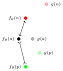
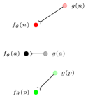
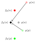
(a) symmetric	(b) regression	(c) relational	(d) asymmetric (this work)

Figure 1: Metric learning and knowledge transfer. (a) Symmetric: Positive (negative) pairs of examples mutually attracted (repulsed) in student space; teacher not used.(b) Regression (absolute ML+KD [81]): Examples in student space attracted to corresponding examples in teacher space; labels not used. (c) Relational (relative ML+KD [81] or distance-wise RKD [47]): Distances encouraged to be the same in both spaces; labels not used. (d) Asymmetric (this work): Anchors in student space attracted to (repulsed from) positives (negatives) in teacher space; both labels and teacher used.

Figure 1 illustrates the idea. When used with loss functions discussed in subsection 3.3, (3) (Figure 1(d)) uses both the labels and the teacher, essentially combining metric learning and knowledge transfer. With the same loss functions, (2) (Figure 1(a)) uses the labels only, focusing on metric learning only. Instead, as discussed in subsection 3.4, relational distillation [81, 47] uses the teacher only, focusing on knowledge transfer only (Figure 1(b,c)). In practice, these other solutions require a linear combination of two error functions for metric learning and knowledge transfer.

3.3 Loss functions using labels

When using the labels, we have access to positive and negative examples $P(a)$ and $N(a)$ per anchor $a$. The teacher $g$ may be used in addition to labels or not by using the asymmetric (3) or symmetric (2) similarity, respectively. We write either as $s_{\theta}(a,x)$ below.

Contrastive

The contrastive loss [18] encourages independently positive examples $p$ to be close to the anchor $a$ and negative examples $n$ farther from $a$ by margin $m$ in the student space:

$$\ell_{\mathrm{contr}}(a;\theta)\mathrel{:=}-\sum_{p\in P(a)}s_{\theta}(a,p)+\sum_{n\in N(a)}[s_{\theta}(a,n)-m]_{+}.$$ (4)

Triplet

The triplet loss [70] encourages positive examples $p$ to be closer to the anchor $a$ than negative examples $n$ by margin $m$ in the student space:

$$\ell_{\mathrm{triplet}}(a;\theta)\mathrel{:=}\sum_{(p,n)\in L(a)}[s_{\theta}(a,n)-s_{\theta}(a,p)+m]_{+},$$ (5)

where typically $L(a)\mathrel{:=}P(a)\times N(a)$. Positive and negative examples are not used independently: if similarities are ranked correctly, the corresponding loss term is zero.

Multi-similarity

The multi-similarity loss [71] treats positives and negatives independently:

$$\ell_{\mathrm{MS}}(a;\theta)\mathrel{:=}\frac{1}{\alpha}\log\left(1+\sum_{p\in P(a)}e^{-\alpha(s_{\theta}(a,p)-m)}\right)+\frac{1}{\beta}\log\left(1+\sum_{n\in N(a)}e^{\beta(s_{\theta}(a,n)-m)}\right).$$ (6)

Here, multiple examples are taken into account together by a nonlinear function: positives (negatives) that are farthest from (nearest to) the anchor receive the greatest relative weight.

3.4 Loss functions using the teacher only

When not using the labels, the only source of supervision is the teacher model $g$. Symmetric similarity (2) is not an option here; we either use use (3) or other ways to compare the two models. Given anchor $a$, the loss may depend on $a$ alone, or also the additional examples $U(a)$. We write $S(a,x)\mathrel{:=}\operatorname{sim}(g(a),g(x))$ for the similarity of $a$ and some $x\in U(a)$ in the teacher space.

Regression

The simplest option is regression, encouraging the representations of the same input example $a$ by the two models to be close by using asymmetric similarity (3):

$$\ell_{\mathrm{reg}}(a;\theta)\mathrel{:=}-s_{\theta}^{\mathrm{asym}}(a,a)=-\operatorname{sim}(f_{\theta}(a),g(a)).$$ (7)

For each anchor, it does not depend on any other example. It is the same as the absolute version of metric learning knowledge distillation (ML+KD) [81] and as contrastive loss (4) on asymmetric similarity (3) (using only the anchor as a positive for itself).

Relational distillation

Given an anchor $\mathbf{a}$ and one or more other vectors $\mathbf{x},\dots$ $\in^{d}$, relational knowledge distillation (RKD) [47] is based on a number of relational measurements $\psi(\mathbf{a},\mathbf{x},\dots)$. One such $\psi(\mathbf{a},\mathbf{x},\dots)$ is the distance $\left\|{\mathbf{a}-\mathbf{x}}\right\|$ for $\mathbf{x}\in^{d}$. Another is the angle $\operatorname{sim}(\mathbf{a}-\mathbf{x},\mathbf{a}-\mathbf{y})$ formed by $\mathbf{a},\mathbf{x},\mathbf{y}$, for $\mathbf{x},\mathbf{y}\in^{d}$. The loss is called distance-wise and angle-wise, respectively. The RKD loss encourages the same measurements by both models,

$$\ell_{\mathrm{RKD}}(a;\theta)\mathrel{:=}\sum_{(x,\dots)\in U(a)^{n}}r(\psi(f_{\theta}(a),f_{\theta}(x),\dots),\psi(g(a),g(x),\dots)),$$ (8)

where $n$ is e.g. $1$ for distance and $2$ for angle and $r$ is a regression loss, taken as Huber [47]. RKD encompasses regression by $\psi$ taken as the identity mapping on the anchor feature alone and $r$ taken as $-\operatorname{sim}$. It also encompasses the relative setting of ML+KD [81] by $\psi(\mathbf{a},\mathbf{x})\mathrel{:=}\left\|{\mathbf{a}-\mathbf{x}}\right\|$ and the direct match baseline of DarkRank [9] by $\psi(\mathbf{a},\mathbf{x})\mathrel{:=}\left\|{\mathbf{a}-\mathbf{x}}\right\|^{2}$ .

DarkRank

Let $V(a,x)\mathrel{:=}\{y\in U(a):S(a,y)\leq S(a,x)\}$ be the set of examples in $U(a)$ that are mapped farther away from anchor $a$ than $x$ in the teacher space. For each $x\in U(a)$, DarkRank [9] encourages those examples to be farther away from $a$ than $x$ in the student space:

$$\ell_{\mathrm{DR}}(a;\theta)\mathrel{:=}-\sum_{x\in U(a)}\left(s_{\theta}^{\mathrm{sym}}(a,x)-\log\sum_{y\in V(a,x)}e^{s_{\theta}^{\mathrm{sym}}(a,y)}\right)$$ (9)

It is an application of the listwise loss [7, 76], where the ground truth ranking is obtained by the teacher rather than some form of annotation.

4 Experiments

4.1 Setup

Datasets

We use the SfM dataset [53] for training, containing 133k images for training and 30k images for validation. We use the revisited $\mathcal{R}$Oxford5k and $\mathcal{R}$Paris6k datasets [51] for testing, each having 70 query images. All datasets depict particular architectural landmarks under very diverse viewing conditions. We follow the standard evaluation protocol, using the medium and hard settings [51]. We report mean average precision (mAP), including mean precision at 10 (mP@10) in the supplementary material. Comparisons are based on mAP. To compare with pruning [73], we also use the original Oxford5k [49] and Paris6k [50] datasets, reporting mAP only.

Networks

All models are pre-trained for classification on ImageNet [56] and then fine-tuned for image retrieval on SfM, following the setup of the same work. We use VGG-16 [60] and ResNet101 [22] as teacher models with the feature dimensionality $d$ of 512 and 2048, respectively. We use MobileNetV2 [57] and EfficientNet-B3 [63] as student networks, removing any fully connected layers and stacking one $1\times 1$ convolutional layer to match the dimensionality of the teacher. All networks use generalized mean-pooling (GeM) [53] on the last convolutional feature map.

Implementation details

The image resolution is limited to $362\times 362$ at training (fine-tuning). At testing, a multi-scale representation is used, with initial resolution of $1024\times 1024$ and scale factors of 1, $\frac{1}{\sqrt{2}}$ and $\frac{1}{2}$. The representation is pooled by GeM over the features of the three scaled inputs. We use supervised whitening, trained on the same SfM dataset [53]. In asymmetric testing, whitening is learned in the teacher space. Our implementation is based on the official code of [53] in PyTorch, as well as [71, 47, 9]. Teacher models are taken from [53].

Training and hyper-parameters

We follow the training setup of [53] for loss functions that use labels. We use the validation set to determine the hyperparameter values and the best model. We train all models using the SGD with learning rate decay of 0.99 per epoch. Symmetric training (2) takes place for 100 epochs or until convergence based on the validation set. For asymmetric training (3), this is extended to 300 epochs. Each epoch consists of 2000 tuples. A mini-batch has 10 tuples, each composed of 1 anchor, 1 corresponding positive and 5 negatives. For unsupervised losses we create tuples of the same overall size. We use weight decay of $10^{-6}$ in each experiment.

Loss functions

For contrastive loss (4), we set the margin $m=0.7$ and the initial learning rate $\eta$ to $10^{-5}$ and $10^{-3}$ for symmetric and asymmetric training, respectively. For triplet (5), we set $m=0.1$ and $\eta=10^{-8}$ . For multi-similarity (6) we set $m=0.6$, $\alpha=1$, $\beta=1$ and $\eta=10^{-8}$ for all setups. For regression (7), we set $\eta=10^{-3}$. We use the DA variant or RKD [47] (8), with the angle-wise and distance-wise loss weighted by a factor of 2 and 1 respectively, and $\eta=10^{-2}$. For DarkRank (DR) (9), we set $\eta=10^{-6}$ for the VGG16 teacher; for ResNet101, $\eta=10^{-5}$ for MobileNetV2 and $\eta=10^{-7}$ for EfficientNet-B3. We do not discriminate between the student training being supervised or not, since labels are already used for teacher training.

Mining

When using labels, we use hard negative mining as a default, following [53]. Negatives are mined each epoch from a random subset of 22k images of the training set. The negatives closest to the anchor (according to (2) or (3), depending on the setting) are selected. There is no mining for positives, because there are only few (1-2) positives per anchor. When not using labels, we draw additional examples uniformly at random as a default. There is no mining for regression.

4.2 Results

Student	Teacher		Lab	Loss	Self	Pos	Neg	Mining		Symmetric Testing				Asymmetric Testing
									Asym	Medium		Hard		Medium		Hard
										$\mathcal{R}$Oxf	$\mathcal{R}$Par	$\mathcal{R}$Oxf	$\mathcal{R}$Par	$\mathcal{R}$Oxf	$\mathcal{R}$Par	$\mathcal{R}$Oxf	$\mathcal{R}$Par
MobileNetV2	VGG16		✓	Contr (4)		✓	✓	hard	✓	57.3	67.1	31.1	41.3	38.3	49.8	18.4	23.8
			✓	Contr (4)	✓	✓	✓	hard	✓	57.3	68.4	31.5	42.2	42.9	55.9	22.6	31.4
			✓	Contr (4)		✓		hard	✓	55.9	66.7	31.1	40.6	34.1	47.3	17.0	24.5
			✓	Contr (4)	✓	✓		hard	✓	55.5	67.0	30.4	40.9	38.2	52.2	15.3	28.9
				Reg (7)	✓			–	✓	53.3	67.5	28.9	40.9	48.0	57.9	26.5	32.6

Table 1: Contrastive–regression ablation. Symmetric and asymmetric testing mAP on $\mathcal{R}$Oxford5k and $\mathcal{R}$Paris6k [51]. Lab: using labels in student model training. Pos, Neg: Using positives, negatives. Self: Using anchor (by teacher) as positive for itself (by student). Asym: Using asymmetric similarity (3) at training. The second row is an option that we call Contr⁺. GeM pooling and learned whitening [53] used in all cases.

Contrastive–regression ablation

As will be shown in the following results, contrastive loss and regression turn out be most effective in general. Moreover, by comparing (4) with (7), contrastive with asymmetric similarity (3) encompasses regression by setting each anchor as a positive for itself, without any other positive or negatives. To better understand the relation between these two loss functions, we perform an ablation study where we investigate versions of contrastive on (3) having negatives, or not, and the anchor itself as positive, or not. The results are shown in Table 1 for VGG16$\to$MobileNetV2. In symmetric testing, it turns out that the best combination is having both negatives and the anchor itself. The same happens in almost all cases for other teacher and student models, as shown in the supplementary material. We denote this combination as Contr⁺ and we include it in subsequent results. Asymmetric testing is much more challenging. The best is regression in this case, but Contr⁺ is still the second best.

Student		$d$	Teacher		Lab	Loss	Mining		Symmetric Testing				Asymmetric Testing
								Asym	Medium		Hard		Medium		Hard
									$\mathcal{R}$Oxf	$\mathcal{R}$Par	$\mathcal{R}$Oxf	$\mathcal{R}$Par	$\mathcal{R}$Oxf	$\mathcal{R}$Par	$\mathcal{R}$Oxf	$\mathcal{R}$Par
VGG16 [53]		512			✓	Contr (4)	hard		60.9	69.3	32.9	44.2
ResNet101 [53]		2048			✓	Contr (4)	hard		65.4	76.7	40.1	55.2
MobileNetV2		512			✓	Contr (4)	hard		53.6	66.4	28.8	39.7
		2048			✓	Contr (4)	hard		56.1	68.5	30.3	42.0
EfficientNet-B3		512			✓	Contr (4)	hard		53.8	70.9	26.2	46.0
		2048			✓	Contr (4)	hard		59.6	75.1	33.3	51.9
MobileNetV2		512	VGG16		✓	Contr+	hard	✓	57.3	68.4	31.5	42.2	42.9	55.9	22.6	31.4
					✓	Contr (4)	hard	✓	57.3	67.1	31.1	41.3	38.3	49.8	18.4	23.8
					✓	Triplet (5)	hard	✓	37.0	62.4	11.8	36.0	1.8	4.3	0.7	2.8
					✓	MS (6)	hard	✓	36.8	62.8	11.5	36.5	1.9	4.3	0.8	2.7
						Reg (7)	–	✓	53.3	67.5	28.9	40.9	48.0	57.9	26.5	32.6
						RKD (8)	random		46.2	64.3	21.8	37.6	2.0	4.1	0.8	2.6
						DR (9)	random		45.2	60.6	24.6	33.1	1.7	3.8	0.7	2.4
		2048	ResNet101		✓	Contr+	hard	✓	63.2	75.0	37.9	52.0	47.1	61.5	21.8	37.7
					✓	Contr (4)	hard	✓	60.8	72.1	36.1	47.6	32.3	51.5	9.6	28.2
					✓	Triplet (5)	hard	✓	45.5	68.0	19.6	43.4	1.3	3.7	0.7	2.4
					✓	MS (6)	hard	✓	44.5	68.1	17.9	43.2	1.4	3.6	0.7	2.3
						Reg (7)	–	✓	59.8	73.1	35.7	49.5	49.2	65.0	23.3	40.7
						RKD (8)	random		56.1	69.8	31.8	44.2	1.6	4.1	0.8	2.5
						DR (9)	random		48.3	58.0	23.3	31.5	1.3	4.1	0.6	2.7
EfficientNet-B3		512	VGG16		✓	Contr+	hard	✓	56.9	69.0	31.1	43.5	44.7	58.0	23.9	32.4
					✓	Contr (4)	hard	✓	56.8	70.4	31.2	45.4	43.8	24.9	23.0	6.1
					✓	Triplet (5)	hard	✓	33.7	64.6	8.0	40.3	1.4	4.0	0.6	2.5
					✓	MS (6)	hard	✓	33.9	64.9	8.1	40.6	1.4	3.9	0.6	2.5
						Reg (7)	–	✓	55.0	69.4	27.1	44.5	49.4	58.2	26.0	33.0
						RKD (8)	random		51.6	67.6	26.2	41.7	1.3	3.8	0.6	2.5
						DR (9)	random		34.7	61.1	8.5	35.2	1.4	3.9	0.6	2.4
		2048	ResNet101		✓	Contr+	hard	✓	66.8	77.1	42.5	55.5	45.2	63.7	19.6	40.9
					✓	Contr (4)	hard	✓	66.3	77.4	41.3	55.5	37.4	57.4	10.9	33.7
					✓	Triplet (5)	hard	✓	39.5	69.4	11.6	45.8	1.5	4.0	0.7	2.5
					✓	MS (6)	hard	✓	39.9	69.7	11.7	46.2	1.5	4.0	0.7	2.4
						Reg (7)	–	✓	64.9	74.4	40.5	52.4	52.9	65.2	27.8	42.4
						RKD (8)	random		56.3	73.0	30.5	46.4	1.6	3.8	0.7	2.4
						DR (9)	random		40.3	69.9	11.8	46.4	1.5	4.0	0.7	2.5

Table 2: Symmetric and asymmetric testing mAP on $\mathcal{R}$Oxford5k and $\mathcal{R}$Paris6k [51]. Lab: using labels in student model training. Asym: Using asymmetric similarity (3) at training (our work). Contr⁺ is defined in Table 1. Best result highlighted per teacher-student pair. GeM pooling and learned whitening [53] used in all cases.

Symmetric testing

According to the left part of Table 2, Contr⁺ works best on MobileNetV2, while on EfficientNet, either contrastive and Contr⁺ works best, with the two options having little difference. The difference to other loss functions using labels is large, reaching 20% or even 30% on $\mathcal{R}$Oxford5k. Triplet is known to be inferior to contrastive [53], but the difference is more pronounced in our knowledge transfer setting. This result is particularly surprising for multi-similarity, which is state of the art in fine-grained classification [71]. Also surprisingly, regression works best among loss functions not using labels, including recent knowledge transfer methods RKD [47] and DarkRank [9]. It is second or third best in all cases. This finding is contrary to [81], where the regression baseline is found inferior. DarkRank is inferior to RKD, in agreement with [47].

The superiority of contrastive or Contr⁺ over regression confirms that, by using our asymmetric similarity, the original metric learning task is still beneficial. Unlike knowledge distillation on classification tasks, knowledge transfer alone is not the best option. Focusing on the best results (contrastive or Contr⁺), we confirm that, with just one exception (VGG16$\to$EfficientNet on $\mathcal{R}$Paris6k hard), knowledge transfer always helps compared to training without the teacher, using the same $d$. The gain is more pronounced, reaching 7-10% on ResNet101$\to$MobileNetV2, when the teacher is stronger and the student is weaker (the exception corresponds to the weakest teacher and strongest student). MobileNetV2 performs only 2-3% below its teacher. Remarkably, EfficientNet outperforms its teacher: this happens on $\mathcal{R}$Paris6k for VGG16 and on all settings for ResNet101.

Asymmetric testing

Here, similarities are asymmetric at testing, with the database being represented by the teacher and queries by the student. According to the right part of Table 2, regression is the clear winner in this case. This is contrary to [59], where regression fails. In a sense, this can be expected since the student should learn to map images to features exactly like the teacher. Contr⁺ is clearly the second best, with the differences varying between 1-2% on $\mathcal{R}$Paris6k and up to 8% on $\mathcal{R}$Oxford5k. Contrastive is the third, with a further loss of roughly 5-10% or more. Knowledge transfer of weak information like relations or ranking fails completely in this case, which is totally expected. What is unexpected is that triplet and multi-similarity fail too.

When compared with symmetric testing using the corresponding teacher alone, the loss of using the student on queries is 8-16%. There is no substantial difference in this behavior between MobileNetV2 and EfficientNet. Asymmetric testing is considerably more challenging than symmetric. The closest work in terms of asymmetric testing is feature translation [27], where a shallow translator is learned instead of fine-tuning the student end-to-end. This approach performs poorly, with up to 40% mAP loss. Students are still large networks, so there is no computational gain.

Student	%FLOPS	%Param	Teacher	Lab	Loss	mAP
						Oxf	Par
VGG16 [53]	100	100		✓	Contr (4)	82.45	81.37
VGG16-PLFP [73]	57.37	61.05		✓	Contr (4)	76.20	73.18
MobileNetV2	2.44	19.58	VGG16	✓	Contr (4)	74.14	78.26
					Reg (7)	66.58	74.45
	3.14	32.97	ResNet101	✓	Contr (4)	75.30	83.23
					Reg (7)	63.57	76.96

Table 3: Symmetric testing mAP on Paris6k and Oxford5k. FLOPS and parameters relative to VGG16. Lab: using labels in student model training. Using asymmetric similarity (3) in all teacher-student settings. GeM pooling [53] used in all cases but not learned whitening.

Results on Paris6k and Oxford5k

We consider this experiment primarily for comparison with progressive local filter pruning (PLFP) [73], which performs symmetric testing with a pruned version of VGG16. For the sake of comparison, there is no whitening in this case. According to Table 3, MobileNetV2 has substantially lower FLOPS and parameters than the pruned VGG16, yet with either teacher it performs better on Paris and nearly the same on Oxford. EfficientNet, reported in the supplementary material, performs best, although it has more parameters.

5 Conclusions

There are certain unexpected or surprising findings in this work. First, regression is particularly effective in knowledge transfer. It appears that the more the constraints on student mappings (e.g. ranking $\to$ distance/angle relations $\to$ positions), the better the performance in standard symmetric testing. Second, the standard contrastive loss is particularly effective with asymmetric similarity at training, outperforming by a large margin state of the art methods like multi-similarity. A straightforward combination with regression—treating the anchor itself as positive—performs best on symmetric testing. In the new asymmetric testing task, regression is unsurprisingly a winner.

We have shown that using the original metric learning task while transferring knowledge is still beneficial in symmetric testing. It remains to be investigated whether the same can happen in asymmetric testing. We consider the same dataset in teacher and student training, so the latter is as supervised as the former. An interesting extension would be to consider a different, unlabeled dataset in student training. This would be a semi-supervised solution, like data distillation [54].

Appendix A Example of asymmetric hard example mining

Depending on the similarity we use in the loss function, i.e., symmetric (2) or asymmetric(3), we follow the same choice for hard negative mining. This means that, in mining based on asymmetric similarity, the features of anchor $a$ come from the student model $f_{\theta}(a)$ while the database is represented by the teacher $g$. The database is fixed and does not need to be re-computed after each epoch. Only the anchors are updated, which makes training more efficient. Figure 2 gives an example of the hard negatives mined for one anchor across different epochs. Before the training starts (epoch 0) the results are not very informative, which is not surprising giving that the feature spaces of the teacher and the student do not match. However, after just a few epochs we see harder negatives being selected. This example illustrates how asymmetric similarity acts as a knowledge transfer mechanism from the teacher to the student model.

Appendix B Model complexity and parameters

Table 4 gives the number of parameters and computational complexity (in FLOPS) for the networks used in this work. This includes two teachers. It is important to note that the versions of the teachers are already for image retrieval by removing the fully connected layers, hence this version of VGG16 has significantly fewer parameters than the original (around 138M). For the student networks, after removing the fully connected layers, a $1\times 1$ convolutional layer is added to match the output dimensionality of the teacher network. Those models are shown in Table 4 as well as a version of the student model without the additional convolutional layer and fully connected layers.

Network	Teacher	d	GFLOPS	Param(M)
VGG16 [53]		512	79.40	14.71
ResNet101 [53]		2048	42.85	42.50
MobileNetV2		1280	1,74	2.22
	VGG16	512	1.94	2.88
	ResNet101	2048	2.50	4.85
EfficientNet-B3		1536	5.36	10.70
	VGG16	512	5.56	11.48
	ResNet101	2048	6.26	13.84

Table 4: FLOPS and parameters for the networks used in this work. In the top segment, the teacher networks are adapted for image retrieval, i.e. the fully connected layers are removed. The bottom segment shows the student network adapted in the same way and also with an added layer (or not) to match the output dimensionality of the teacher.

Appendix C More results

Complete contrastive–regression ablation

Here, we present the full version of the results of the ablation from Table 1, for all four student-teacher combinations. Apart from mAP, we also report mP@10. Table 5 and Table 6 present the symmetric and asymmetric testing results, respectively. All results agree with the results of Table 1. For symmetric testing, contrastive loss with a single positive and no negatives is again the worst. The addition of the anchor as a positive for itself as well as the negatives improve the results substantially. Contr⁺, which uses both, performs best in most cases with the exception of VGG16$\to$EfficientNet. For asymmetric testing, regression is the best. The inclusion of the anchor as positive for itself gives better results than without it.

Epoch	$a$		$N(a)$
0
5
10
300

Figure 2: Asymmetric hard negative mining. One anchor $a$ shown on the first column, followed by the hard negatives $N(a)$ mined for this anchor, over different epochs. The anchor is represented by the student and the database of potential negatives by the teacher.

Student		$d$	Teacher	Lab	Loss	Self	Pos	Neg	Mining	Medium				Hard
										$\mathcal{R}$Oxford5k		$\mathcal{R}$Paris6k		$\mathcal{R}$Oxford5k		$\mathcal{R}$Paris6k
										mAP	mP@10	mAP	mP@10	mAP	mP@10	mAP	mP@10
MobileNetV2		512	VGG16	✓	Contr (4)		✓	✓	hard	57.3	77.1	67.1	95.7	31.1	47.3	41.3	80.4
				✓	Contr (4)	✓	✓	✓	hard	57.3	78.4	68.4	96.1	31.5	46.9	42.2	78.9
				✓	Contr (4)		✓		hard	55.9	79.2	66.7	95.0	31.1	44.0	40.6	78.9
				✓	Contr (4)	✓	✓		hard	55.5	76.1	67.0	96.0	30.4	44.1	40.9	81.4
					Reg (7)	✓			–	53.3	75.1	67.5	95.6	28.9	43.6	40.9	81.3
		2048	ResNet101	✓	Contr (4)		✓	✓	hard	60.8	81.7	72.1	97.3	36.1	50.4	47.6	85.1
				✓	Contr (4)	✓	✓	✓	hard	63.2	84.4	75.0	98.0	37.9	52.1	52.0	87.3
				✓	Contr (4)		✓		hard	51.8	72.5	67.6	96.0	27.6	38.1	41.3	80.0
				✓	Contr (4)	✓	✓		hard	60.6	80.0	74.1	97.0	35.7	49.4	50.9	85.6
					Reg (7)	✓			–	59.8	80.3	73.1	96.9	35.7	49.4	49.5	84.7
EfficientNet-B3		512	VGG16	✓	Contr (4)		✓	✓	hard	56.8	75.7	70.4	96.3	31.2	43.9	45.4	81.7
				✓	Contr (4)	✓	✓	✓	hard	56.9	75.6	69.0	96.0	31.1	46.7	43.5	80.9
				✓	Contr (4)		✓		hard	56.1	77.0	69.3	96.4	30.1	42.1	44.7	78.4
				✓	Contr (4)	✓	✓		hard	57.6	78.3	69.9	96.9	31.4	46.7	44.9	82.6
					Reg (7)	✓			–	55.0	75.0	69.4	96.6	27.1	42.3	44.5	80.4
		2048	ResNet101	✓	Contr (4)		✓	✓	hard	66.3	85.3	77.4	98.4	41.3	58.9	55.5	88.3
				✓	Contr (4)	✓	✓	✓	hard	66.8	84.7	77.1	98.6	42.5	58.7	55.5	87.9
				✓	Contr (4)		✓		hard	61.7	81.7	74.3	97.1	36.1	51.7	51.6	85.9
				✓	Contr (4)	✓	✓		hard	63.8	83.1	75.9	98.3	40.1	54.3	54.4	87.1
					Reg (7)	✓			–	64.9	83.7	74.4	97.7	40.5	55.9	52.4	87.1

Table 5: Complete contrastive–regression ablation: symmetric testing on $\mathcal{R}$Oxford5k and $\mathcal{R}$Paris6k [51]. Lab: using labels in student model training. Pos, Neg: Using positives, negatives. Self: Using anchor (by teacher) as positive for itself (by student). Using asymmetric similarity (3) at training in all cases. Best mAP highlighted per teacher-student pair. GeM pooling and learned whitening [53] used in all cases.

Student		$d$	Teacher	Lab	Loss	Self	Pos	Neg	Mining	Medium				Hard
										$\mathcal{R}$Oxford5k		$\mathcal{R}$Paris6k		$\mathcal{R}$Oxford5k		$\mathcal{R}$Paris6k
										mAP	mP@10	mAP	mP@10	mAP	mP@10	mAP	mP@10
MobileNetV2		512	VGG16	✓	Contr (4)		✓	✓	hard	38.3	53.7	49.8	84.4	18.4	32.8	23.8	55.7
				✓	Contr (4)	✓	✓	✓	hard	42.9	59.1	55.9	88.4	22.6	35.2	31.4	66.3
				✓	Contr (4)		✓		hard	34.1	48.9	47.3	82.0	17.0	25.6	24.5	53.4
				✓	Contr (4)	✓	✓		hard	38.2	52.0	52.2	86.0	15.3	26.2	28.9	64.1
					Reg (7)	✓			–	48.0	64.3	57.9	90.7	26.5	37.9	32.6	67.1
		2048	ResNet101	✓	Contr (4)		✓	✓	hard	32.3	49.7	51.5	83.3	9.6	18.3	28.2	62.4
				✓	Contr (4)	✓	✓	✓	hard	47.1	65.4	61.5	92.6	21.8	33.1	37.7	74.1
				✓	Contr (4)		✓		hard	27.3	38.4	47.7	80.9	8.4	15.3	24.3	50.6
				✓	Contr (4)	✓	✓		hard	40.5	58.2	55.8	87.6	17.4	26.3	29.9	63.4
					Reg (7)	✓			–	49.2	67.9	65.0	92.6	23.3	36.9	40.7	72.1
EfficientNet-B3		512	VGG16	✓	Contr (4)		✓	✓	hard	43.8	74.7	24.9	39.3	23.0	51.3	6.1	15.6
				✓	Contr (4)	✓	✓	✓	hard	44.7	61.5	58.0	93.3	23.9	37.9	32.4	69.1
				✓	Contr (4)		✓		hard	32.4	45.4	47.8	84.4	14.1	22.0	25.8	56.3
				✓	Contr (4)	✓	✓		hard	41.6	57.5	53.9	90.1	20.3	30.6	30.2	64.0
					Reg (7)	✓			–	49.4	70.0	58.2	92.4	26.0	39.6	33.0	70.6
		2048	ResNet101	✓	Contr (4)		✓	✓	hard	37.4	56.8	57.4	90.4	10.9	24.6	33.7	65.9
				✓	Contr (4)	✓	✓	✓	hard	45.2	67.2	63.7	92.1	19.6	35.5	40.9	73.6
				✓	Contr (4)		✓		hard	30.8	44.5	51.2	83.7	10.2	16.1	27.8	57.0
				✓	Contr (4)	✓	✓		hard	40.1	56.7	59.1	91.1	14.6	24.3	35.0	71.0
					Reg (7)	✓			–	52.9	71.8	65.2	93.3	27.8	41.5	42.4	71.9

Table 6: Complete contrastive–regression ablation: asymmetric testing on $\mathcal{R}$Oxford5k and $\mathcal{R}$Paris6k [51]. Lab: using labels in student model training. Pos, Neg: Using positives, negatives. Self: Using anchor (by teacher) as positive for itself (by student). Using asymmetric similarity (3) at training in all cases. Best mAP highlighted per teacher-student pair. GeM pooling and learned whitening [53] used in all cases.

Student		$d$	Teacher		Lab	Loss	Mining		Medium				Hard
								Asym	$\mathcal{R}$Oxf		$\mathcal{R}$Par		$\mathcal{R}$Oxf		$\mathcal{R}$Par
									mAP	mP@10	mAP	mP@10	mAP	mP@10	mAP	mP@10
VGG16		512			✓	Contr (4)	hard		60.9	81.9	69.3	97.4	32.9	50.9	44.2	83.1
ResNet101		2048			✓	Contr (4)	hard		65.4	85.7	76.7	98.4	40.1	56.6	55.2	87.7
MobileNetV2		512			✓	Contr (4)	hard		53.6	75.8	66.4	96.7	28.8	42.9	39.7	79.0
		2048			✓	Contr (4)	hard		56.1	79.0	68.5	98.1	30.3	46.0	42.0	82.6
EfficientNet-B3		512			✓	Contr (4)	hard		53.8	76.6	70.9	96.6	26.2	42.3	46.0	83.7
		2048			✓	Contr (4)	hard		59.6	86.1	75.1	95.1	33.3	46.0	51.9	87.6
MobileNetV2		512	VGG16		✓	Contr+	hard	✓	57.3	78.4	68.4	96.1	31.5	46.9	42.2	78.9
					✓	Contr (4)	hard	✓	57.3	77.1	67.1	95.7	31.1	47.3	41.3	80.4
					✓	Triplet (5)	hard	✓	37.0	55.2	62.4	94.4	11.8	23.0	36.0	73.7
					✓	MS (6)	hard	✓	36.8	55.2	62.8	94.4	11.5	22.2	36.5	75.0
						Reg (7)	–	✓	53.3	75.1	67.5	95.6	28.9	43.6	40.9	81.3
						RKD (8)	random		46.2	68.1	64.3	94.7	21.8	32.8	37.6	72.3
						DR (9)	random		45.2	66.5	60.6	92.1	24.6	34.9	33.1	74.1
		2048	ResNet101		✓	Contr+	hard	✓	63.2	84.4	75.0	98.0	37.9	52.1	52.0	87.3
					✓	Contr (4)	hard	✓	60.8	81.7	72.1	97.3	36.1	50.4	47.6	85.1
					✓	Triplet (5)	hard	✓	45.5	66.1	68.0	96.1	19.6	33.5	43.4	80.6
					✓	MS (6)	hard	✓	44.5	65.4	68.1	96.1	17.9	32.1	43.2	80.1
						Reg (7)	–	✓	59.8	80.3	73.1	96.9	35.7	49.4	49.5	84.7
						RKD (8)	random		56.1	79.3	69.8	96.3	31.8	46.0	44.2	82.3
						DR (9)	random		48.3	69.8	58.0	94.3	23.3	33.3	31.5	71.4
EfficientNet-B3		512	VGG16		✓	Contr+	hard	✓	56.9	75.6	69.0	96.0	31.1	46.7	43.5	80.9
					✓	Contr (4)	hard	✓	56.8	75.7	70.4	96.3	31.2	43.9	45.4	81.7
					✓	Triplet (5)	hard	✓	33.7	48.5	64.6	94.4	8.0	20.1	40.3	76.1
					✓	MS (6)	hard	✓	33.9	49.5	64.9	94.4	8.1	20.4	40.6	76.9
						Reg (7)	–	✓	55.0	75.0	69.4	96.6	27.1	42.3	44.5	80.4
						RKD (8)	random		51.6	71.4	67.6	95.3	26.2	38.5	41.7	81.1
						DR (9)	random		34.7	50.0	61.1	93.1	8.5	17.8	35.2	67.1
		2048	ResNet101		✓	Contr+	hard	✓	66.8	84.7	77.1	98.6	42.5	58.7	55.5	87.9
					✓	Contr (4)	hard	✓	66.3	85.3	77.4	98.4	41.3	58.9	55.5	88.3
					✓	Triplet (5)	hard	✓	39.5	57.3	69.4	95.9	11.6	24.3	45.8	81.1
					✓	MS (6)	hard	✓	39.9	57.4	69.7	95.7	11.7	24.2	46.2	81.4
						Reg (7)	–	✓	64.9	83.7	74.4	97.7	40.5	55.9	52.4	87.1
						RKD (8)	random		56.3	75.8	73.0	98.4	30.5	46.4	46.4	82.3
						DR (9)	random		40.3	58.4	69.9	95.9	11.8	24.6	46.4	81.1

Table 7: Symmetric testing on $\mathcal{R}$Oxford5k and $\mathcal{R}$Paris6k [51]. Lab: using labels in student model training. Asym: Using asymmetric similarity (3) at training. Best mAP highlighted per teacher-student pair. GeM pooling and learned whitening [53] used in all cases.

Complete symmetric and asymmetric testing results

Table 7 supplements Table 2 by adding mP@10 scores for all the symmetric testing experiments. Similarly, Table 8 adds mP@10 results to all asymmetric testing experiments. Overall, the conclusions made based on mAP apply to the mP@10 results.

Student		$d$	Teacher		Lab	Loss	Mining		Medium				Hard
								Asym	$\mathcal{R}$Oxf		$\mathcal{R}$Par		$\mathcal{R}$Oxf		$\mathcal{R}$Par
									mAP	mP@10	mAP	mP@10	mAP	mP@10	mAP	mP@10
VGG16		512			✓	Contr (4)	hard		60.9	81.9	69.3	97.4	32.9	50.9	44.2	83.1
ResNet101		2048			✓	Contr (4)	hard		65.4	85.7	76.7	98.4	40.1	56.6	55.2	87.7
MobileNetV2		512			✓	Contr (4)	hard		53.6	75.8	66.4	96.7	28.8	42.9	39.7	79.0
		2048			✓	Contr (4)	hard		56.1	79.0	68.5	98.1	30.3	46.0	42.0	82.6
EfficientNet-B3		512			✓	Contr (4)	hard		53.8	76.6	70.9	96.6	26.2	42.3	46.0	83.7
		2048			✓	Contr (4)	hard		59.6	86.1	75.1	95.1	33.3	46.0	51.9	87.6
MobileNetV2		512	VGG16		✓	Contr+	hard	✓	42.9	59.1	55.9	88.4	22.6	35.2	31.4	66.3
					✓	Contr (4)	hard	✓	38.3	53.7	49.8	84.4	18.4	32.8	23.8	55.7
					✓	Triplet (5)	hard	✓	1.8	0.0	4.3	1.3	0.7	0.0	2.8	1.4
					✓	MS (6)	hard	✓	1.9	0.0	4.3	1.6	0.8	0.0	2.7	1.6
						Reg (7)	–	✓	48.0	64.3	57.9	90.7	26.5	37.9	32.6	67.1
						RKD (8)	random		2.0	0.0	4.1	1.0	0.8	0.0	2.6	1.0
						DR (9)	random		1.7	0.0	3.8	0.3	0.7	0.0	2.4	0.3
		2048	ResNet101		✓	Contr+	hard	✓	47.1	65.4	61.5	92.6	21.8	33.1	37.7	74.1
					✓	Contr (4)	hard	✓	32.3	49.7	51.5	83.3	9.6	18.3	28.2	62.4
					✓	Triplet (5)	hard	✓	1.3	0.0	3.7	1.4	0.7	0.0	2.4	1.4
					✓	MS (6)	hard	✓	1.4	0.3	3.6	1.0	0.7	0.3	2.3	0.9
						Reg (7)	–	✓	49.2	67.9	65.0	92.6	23.3	36.9	40.7	72.1
						RKD (8)	random		1.6	1.3	4.1	2.3	0.8	1.1	2.5	1.6
						DR (9)	random		1.3	0.4	4.1	3.6	0.6	0.3	2.7	3.1
EfficientNet-B3		512	VGG16		✓	Contr+	hard	✓	44.7	61.5	58.0	93.3	23.9	37.9	32.4	69.1
					✓	Contr (4)	hard	✓	43.8	74.7	24.9	39.3	23.0	51.3	6.1	15.6
					✓	Triplet (5)	hard	✓	1.4	0.0	4.0	0.0	0.6	0.0	2.5	0.0
					✓	MS (6)	hard	✓	1.4	0.0	3.9	0.0	0.6	0.0	2.5	0.0
						Reg (7)	–	✓	49.4	70.0	58.2	92.4	26.0	39.6	33.0	70.6
						RKD (8)	random		1.3	0.0	3.8	0.7	0.6	0.0	2.5	0.3
						DR (9)	random		1.4	0.0	3.9	0.0	0.6	0.0	2.4	0.0
		2048	ResNet101		✓	Contr+	hard	✓	45.2	67.2	63.7	92.1	19.6	35.5	40.9	73.6
					✓	Contr (4)	hard	✓	37.4	56.8	57.4	90.4	10.9	24.6	33.7	65.9
					✓	Triplet (5)	hard	✓	1.5	0.7	4.0	1.6	0.7	0.7	2.5	0.9
					✓	MS (6)	hard	✓	1.5	0.7	4.0	1.4	0.7	0.7	2.4	1.0
						Reg (7)	–	✓	52.9	71.8	65.2	93.3	27.8	41.5	42.4	71.9
						RKD (8)	random		1.6	0.7	3.8	1.6	0.7	0.4	2.4	0.7
						DR (9)	random		1.5	0.9	4.0	1.9	0.7	0.9	2.5	1.4

Table 8: Asymmetric testing on $\mathcal{R}$Oxford5k and $\mathcal{R}$Paris6k [51]. Lab: using labels in student model training. Asym: Using asymmetric similarity (3) at training. Best mAP highlighted per teacher-student pair. GeM pooling and learned whitening [53] used in all cases. The results without a teacher in the top block correspond to symmetric testing (same as in Table 7) and are only added here for convenience.

References

- [1] Jimmy Ba and Rich Caruana. Do deep nets really need to be deep? In NIPS, 2014.
- [2] Artem Babenko, Anton Slesarev, Alexandr Chigorin, and Victor Lempitsky. Neural codes for image retrieval. In ECCV, 2014.
- [3] Mikhail Belkin and Partha Niyogi. Laplacian eigenmaps for dimensionality reduction and data representation. Neural computation, 15(6), 2003.
- [4] Oren Boiman, Eli Shechtman, and Michal Irani. In defense of nearest-neighbor based image classification. In CVPR, 2008.
- [5] Fatih Cakir, Kun He, Xide Xia, Brian Kulis, and Stan Sclaroff. Deep metric learning to rank. In CVPR, 2019.
- [6] Xuefei Cao, Bor-Chun Chen, and Ser-Nam Lim. Unsupervised deep metric learning via auxiliary rotation loss. arXiv preprint arXiv:1911.07072, 2019.
- [7] Zhe Cao, Tao Qin, Tie-Yan Liu, Ming-Feng Tsai, and Hang Li. Learning to rank: From pairwise approach to listwise approach. In ICML, 2007.
- [8] Ting Chen, Simon Kornblith, Mohammad Norouzi, and Geoffrey Hinton. A simple framework for contrastive learning of visual representations. arXiv preprint arXiv:2002.05709, 2020.
- [9] Yuntao Chen, Naiyan Wang, and Zhaoxiang Zhang. DarkRank: Accelerating deep metric learning via cross sample similarities transfer. In AAAI, 2018.
- [10] Damek Davis, Jonathan Balzer, and Stefano Soatto. Asymmetric sparse kernel approximations for large-scale visual search. In CVPR, 2014.
- [11] Jiankang Deng, Jia Guo, Niannan Xue, and Stefanos Zafeiriou. ArcFace: Additive angular margin loss for deep face recognition. In CVPR, 2019.
- [12] Wei Dong, Moses Charikar, and Kai Li. Asymmetric distance estimation with sketches for similarity search in high-dimensional spaces. In SIGIR, 2008.
- [13] Fartash Faghri, David J Fleet, Jamie Ryan Kiros, and Sanja Fidler. VSE++: Improving visual-semantic embeddings with hard negatives. arXiv preprint arXiv:1707.05612, 2017.
- [14] Andrea Frome, Greg S Corrado, Jon Shlens, Samy Bengio, Jeff Dean, Marc’Aurelio Ranzato, and Tomas Mikolov. Devise: A deep visual-semantic embedding model. In NIPS, 2013.
- [15] Yunchao Gong, Liu Liu, Ming Yang, and Lubomir Bourdev. Compressing deep convolutional networks using vector quantization. arXiv preprint arXiv:1412.6115, 2014.
- [16] Albert Gordo, Jon Almazan, Jerome Revaud, and Diane Larlus. Deep image retrieval: Learning global representations for image search. ECCV, 2016.
- [17] Albert Gordo and Florent Perronnin. Asymmetric distances for binary embeddings. In CVPR, 2011.
- [18] Raia Hadsell, Sumit Chopra, and Yann Lecun. Dimensionality reduction by learning an invariant mapping. In CVPR, 2006.
- [19] Xufeng Han, Thomas Leung, Yangqing Jia, Rahul Sukthankar, and Alexander C Berg. MatchNet: Unifying feature and metric learning for patch-based matching. In CVPR, 2015.
- [20] Ben Harwood, Vijay Kumar B G, Gustavo Carneiro, Ian Reid, and Tom Drummond. Smart mining for deep metric learning. In ICCV, 2017.
- [21] Kaiming He, Haoqi Fan, Yuxin Wu, Saining Xie, and Ross Girshick. Momentum contrast for unsupervised visual representation learning. arXiv preprint arXiv:1911.05722, 2019.
- [22] Kaiming He, Xiangyu Zhang, Shaoqing Ren, and Jian Sun. Deep residual learning for image recognition. In CVPR, 2016.
- [23] Geoffrey Hinton, Oriol Vinyals, and Jeff Dean. Distilling the knowledge in a neural network. arXiv preprint arXiv:1503.02531, 2015.
- [24] Elad Hoffer, Itay Hubara, and Daniel Soudry. Fix your classifier: the marginal value of training the last weight layer. arXiv preprint arXiv:1801.04540, 2018.
- [25] Andrew Howard, Mark Sandler, Grace Chu, Liang-Chieh Chen, Bo Chen, Mingxing Tan, Weijun Wang, Yukun Zhu, Ruoming Pang, Vijay Vasudevan, et al. Searching for MobileNetV3. In ICCV, 2019.
- [26] Andrew G Howard, Menglong Zhu, Bo Chen, Dmitry Kalenichenko, Weijun Wang, Tobias Weyand, Marco Andreetto, and Hartwig Adam. MobileNets: Efficient convolutional neural networks for mobile vision applications. arXiv preprint arXiv:1704.04861, 2017.
- [27] Jie Hu, Rongrong Ji, Hong Liu, Shengchuan Zhang, Cheng Deng, and Qi Tian. Towards visual feature translation. In CVPR, 2019.
- [28] Gao Huang, Zhuang Liu, Laurens van der Maaten, and Kilian Q. Weinberger. Densely connected convolutional networks. In CVPR, 2017.
- [29] Yanping Huang, Youlong Cheng, Ankur Bapna, Orhan Firat, Dehao Chen, Mia Chen, HyoukJoong Lee, Jiquan Ngiam, Quoc V Le, Yonghui Wu, and Zhifeng Chen. GPipe: Efficient training of giant neural networks using pipeline parallelism. In NIPS, 2019.
- [30] Forrest N Iandola, Song Han, Matthew W Moskewicz, Khalid Ashraf, William J Dally, and Kurt Keutzer. Squeezenet: Alexnet-level accuracy with 50x fewer parameters and <0.5 mb model size. arXiv preprint arXiv:1602.07360, 2016.
- [31] Ahmet Iscen, Giorgos Tolias, Yannis Avrithis, and Ondřej Chum. Mining on manifolds: Metric learning without labels. In CVPR, 2018.
- [32] Mihir Jain, Herve Jégou, and Patrick Gros. Asymmetric hamming embedding. In ACM Multimedia, 2011.
- [33] H. Jégou, M. Douze, and C. Schmid. Improving bag-of-features for large scale image search. IJCV, 87(3), 2010.
- [34] H. Jégou, M. Douze, and C. Schmid. Product quantization for nearest neighbor search. PAMI, 33(1):117–128, 2011.
- [35] H. Jégou, H. Harzallah, and C. Schmid. A contextual dissimilarity measure for accurate and efficient image search. In CVPR, 2007.
- [36] Hervé Jégou and Andrew Zisserman. Triangulation embedding and democratic kernels for image search. In CVPR, 2014.
- [37] Jaechul Kim and Kristen Grauman. Asymmetric region-to-image matching for comparing images with generic object categories. In CVPR, 2010.
- [38] Sungyeon Kim, Minkyo Seo, Ivan Laptev, Minsu Cho, and Suha Kwak. Deep metric learning beyond binary supervision. In CVPR, 2019.
- [39] Ryan Kiros, Ruslan Salakhutdinov, and Richard S Zemel. Unifying visual-semantic embeddings with multimodal neural language models. arXiv preprint arXiv:1411.2539, 2014.
- [40] Shengcai Liao and Stan Z Li. Efficient PSD constrained asymmetric metric learning for person re-identification. In ICCV, 2015.
- [41] Hanxiao Liu, Karen Simonyan, and Yiming Yang. DARTS: Differentiable architecture search. arXiv preprint arXiv:1806.09055, 2018.
- [42] Zhuang Liu, Mingjie Sun, Tinghui Zhou, Gao Huang, and Trevor Darrell. Rethinking the value of network pruning. In ICLR, 2018.
- [43] D.G. Lowe. Distinctive image features from scale-invariant keypoints. IJCV, 60(2):91–110, 2004.
- [44] Ishan Misra and Laurens van der Maaten. Self-supervised learning of pretext-invariant representations. arXiv preprint arXiv:1912.01991, 2019.
- [45] Behnam Neyshabur, Nati Srebro, Ruslan R Salakhutdinov, Yury Makarychev, and Payman Yadollahpour. The power of asymmetry in binary hashing. In NIPS, 2013.
- [46] Hyun Oh Song, Yu Xiang, Stefanie Jegelka, and Silvio Savarese. Deep metric learning via lifted structured feature embedding. In CVPR, 2016.
- [47] Wonpyo Park, Dongju Kim, Yan Lu, and Minsu Cho. Relational knowledge distillation. In CVPR, 2019.
- [48] Hieu Pham, Melody Y Guan, Barret Zoph, Quoc V Le, and Jeff Dean. Efficient neural architecture search via parameter sharing. arXiv preprint arXiv:1802.03268, 2018.
- [49] J. Philbin, O. Chum, M. Isard, J. Sivic, and A. Zisserman. Object retrieval with large vocabularies and fast spatial matching. In CVPR, 2007.
- [50] James Philbin, Ondrej Chum, Josef Sivic, Michael Isard, and Andrew Zisserman. Lost in quantization: Improving particular object retrieval in large scale image databases. In CVPR, 2008.
- [51] Filip Radenović, Ahmet Iscen, Giorgos Tolias, Yannis Avrithis, and Ondřej Chum. Revisiting oxford and paris: Large-scale image retrieval benchmarking. In CVPR, 2018.
- [52] Filip Radenović, Giorgos Tolias, and Ondřej Chum. CNN image retrieval learns from bow: Unsupervised fine-tuning with hard examples. ECCV, 2016.
- [53] Filip Radenović, Giorgos Tolias, and Ondřej Chum. Fine-tuning CNN image retrieval with no human annotation. PAMI, 41(7):1655–1668, 2018.
- [54] Ilija Radosavovic, Piotr Dollar, Ross Girshick, Georgia Gkioxari, and Kaiming He. Data distillation: Towards omni-supervised learning. In CVPR, 2018.
- [55] Ali Sharif Razavian, Josephine Sullivan, Atsuto Maki, and Stefan Carlsson. Visual instance retrieval with deep convolutional networks. arXiv preprint arXiv:1412.6574, 2014.
- [56] Olga Russakovsky, Jia Deng, Hao Su, Jonathan Krause, Sanjeev Satheesh, Sean Ma, Zhiheng Huang, Andrej Karpathy, Aditya Khosla, Michael Bernstein, et al. ImageNet large scale visual recognition challenge. IJCV, 115(3):211–252, 2015.
- [57] Mark Sandler, Andrew Howard, Menglong Zhu, Andrey Zhmoginov, and Liang-Chieh Chen. Mobilenetv2: Inverted residuals and linear bottlenecks. In CVPR, 2018.
- [58] Bernhard Schölkopf, Alexander Smola, and Klaus-Robert Müller. Nonlinear component analysis as a kernel eigenvalue problem. Neural computation, 10(5):1299–1319, 1998.
- [59] Yantao Shen, Yuanjun Xiong, Wei Xia, and Stefano Soatto. Towards backward-compatible representation learning. arXiv preprint arXiv:2003.11942, 2020.
- [60] Karen Simonyan and Andrew Zisserman. Very deep convolutional networks for large-scale image recognition. arXiv preprint arXiv:1409.1556, 2014.
- [61] Jake Snell, Kevin Swersky, and Richard Zemel. Prototypical networks for few-shot learning. In NIPS, 2017.
- [62] Mingxing Tan, Bo Chen, Ruoming Pang, Vijay Vasudevan, Mark Sandler, Andrew Howard, and Quoc V Le. MnasNet: Platform-aware neural architecture search for mobile. In CVPR, 2019.
- [63] Mingxing Tan and Quoc V Le. EfficientNet: Rethinking model scaling for convolutional neural networks. arXiv preprint arXiv:1905.11946, 2019.
- [64] J. Tenenbaum. Mapping a manifold of perceptual observations. In NIPS. 1997.
- [65] Giorgos Tolias, Yannis Avrithis, and Hervé Jégou. To aggregate or not to aggregate: Selective match kernels for image search. In ICCV, 2013.
- [66] Giorgos Tolias and Ondrej Chum. Asymmetric feature maps with application to sketch based retrieval. In CVPR, 2017.
- [67] Giorgos Tolias, Ronan Sicre, and Hervé Jégou. Particular object retrieval with integral max-pooling of cnn activations. ICLR, 2016.
- [68] Oriol Vinyals, Charles Blundell, Timothy Lillicrap, Koray Kavukcuoglu, and Daan Wierstra. Matching networks for one shot learning. In NIPS, 2016.
- [69] Hao Wang, Yitong Wang, Zheng Zhou, Xing Ji, Dihong Gong, Jingchao Zhou, Zhifeng Li, and Wei Liu. CosFace: Large margin cosine loss for deep face recognition. In CVPR, 2018.
- [70] Jiang Wang, Yang Song, Thomas Leung, Chuck Rosenberg, Jingbin Wang, James Philbin, Bo Chen, and Ying Wu. Learning fine-grained image similarity with deep ranking. In CVPR, 2014.
- [71] Xun Wang, Xintong Han, Weilin Huang, Dengke Dong, and Matthew R Scott. Multi-similarity loss with general pair weighting for deep metric learning. In CVPR, 2019.
- [72] Xun Wang, Haozhi Zhang, Weilin Huang, and Matthew R Scott. Cross-batch memory for embedding learning. arXiv preprint arXiv:1912.06798, 2019.
- [73] Xiaodong Wang, Zhedong Zheng, Yang He, Fei Yan, Zhiqiang Zeng, and Yi Yang. Progressive local filter pruning for image retrieval acceleration. arXiv preprint arXiv:2001.08878, 2020.
- [74] Chao-Yuan Wu, R. Manmatha, Alexander J. Smola, and Philipp Krahenbuhl. Sampling matters in deep embedding learning. In ICCV, 2017.
- [75] Zhirong Wu, Alexei A Efros, and Stella X Yu. Improving generalization via scalable neighborhood component analysis. In ECCV, 2018.
- [76] Fen Xia, Tie-Yan Liu, Jue Wang, Wensheng Zhang, and Hang Li. Listwise approach to learning to rank: theory and algorithm. In ICML, 2008.
- [77] Eric P Xing, Michael I Jordan, Stuart J Russell, and Andrew Y Ng. Distance metric learning with application to clustering with side-information. In NIPS, 2003.
- [78] Xinyi Xu, Yanhua Yang, Cheng Deng, and Feng Zheng. Deep asymmetric metric learning via rich relationship mining. In CVPR, 2019.
- [79] Mang Ye, Xu Zhang, Pong C. Yuen, and Shih-Fu Chang. Unsupervised embedding learning via invariant and spreading instance feature. In CVPR, June 2019.
- [80] Hong-Xing Yu, Ancong Wu, and Wei-Shi Zheng. Cross-view asymmetric metric learning for unsupervised person re-identification. In ICCV, 2017.
- [81] Lu Yu, Vacit Oguz Yazici, Xialei Liu, Joost Van De Weijer, Yongmei Cheng, and Arnau Ramisa. Learning metrics from teachers: Compact networks for image embedding. In CVPR, 2019.
- [82] Sergey Zagoruyko and Nikos Komodakis. Wide residual networks. arXiv preprint arXiv:1605.07146, 2016.
- [83] Xiangyu Zhang, Xinyu Zhou, Mengxiao Lin, and Jian Sun. ShuffleNet: An extremely efficient convolutional neural network for mobile devices. In CVPR, 2018.
- [84] Cai-Zhi Zhu, Herve Jégou, and Shin’ichi Satoh. Query-adaptive asymmetrical dissimilarities for visual object retrieval. In ICCV, 2013.