Effective conductivity of the multidimensional chessboard

Abstract

An algebraic formula for the effective conductivity of a $d$-dimensional, two-component chessboard (checkerboard) is proposed. The derivation relies on the self-duality of the square bond lattice, the principle of universality, and the analytical capabilities of the Walker Diffusion Method.

I introduction

There is long-standing interest in the derivation of exact expressions for the effective conductivity of two-component systems. These of course rely on the symmetries of the system. By consideration of an electric field applied across a two-dimensional (2D) medium that is a square array of identical circular inclusions imbedded in a matrix, Keller (Keller1964, ) showed that

$$\sigma\left(p,\alpha;q,\beta\right)\>\sigma\left(p,\beta;q,\alpha\right)=\alpha\,\beta$$ (1)

where $\sigma\left(p,\alpha;q,\beta\right)$ is the effective conductivity of the system $\left(p,\alpha;q,\beta\right)$, which is the medium with inclusions of conductivity $\alpha$ comprising areal fraction $p$, and matrix of conductivity $\beta$ comprising areal fraction $q=1-p$. Mendelson (Mendelson, ) subsequently showed that this relation holds as well when the inclusions are randomly distributed over the matrix. As in these cases, Eq. (1) pertains to all 2D, two-component, isotropic systems containing a percolating domain. Note that Eq. (1) is unaffected by the exchange $\alpha\leftrightarrow\beta$, which allows all conductivity values $\beta/\alpha\geq 0$.

A derivation of the effective conductivity $\sigma_{dD}$ of the $d$-dimensional, two-component chessboard has not appeared in the literature. The following section derives $\sigma_{2D}$ by utilizing the self-duality property of a 2D chessboard constructed as a square (conducting) bond network. Section III applies an analytic expression of the Walker Diffusion Method (WDM) to construct a formula for $\sigma_{dD}$. That result is assessed in Section IV, by a comparison with an analytical lower bound on $\sigma_{dD}$, and with calculated values for $\sigma_{3D}$, found in the literature. Final comments are made in Section V.

II use of self-duality

The dual of a two-component, 2D square bond lattice is constructed by crossing each $\alpha$ bond in the original system $\left(p,\alpha;q,\beta\right)$ with a $\alpha^{-1}$ bond and crossing each $\beta$ bond with a $\beta^{-1}$ bond. The dual system $\left(p,\alpha^{-1};q,\beta^{-1}\right)$ is again a 2D square bond lattice. Of relevance here is the fact that the conductivity of the original system equals the resistivity of its dual; that is,

$$\sigma\left(p,\alpha;q,\beta\right)\>\sigma\left(p,\alpha^{-1};q,\beta^{-1}\right)=1.$$ (2)

In the particular case of the 2D chessboard (constructed of conducting bonds), this relation becomes

$$\sigma\left(\nicefrac{{1}}{{2}},\alpha;\nicefrac{{1}}{{2}},\beta\right)\>\sigma\left(\nicefrac{{1}}{{2}},\alpha^{-1};\nicefrac{{1}}{{2}},\beta^{-1}\right)=1$$ (3)

or equivalently

$$\sigma\left(\nicefrac{{1}}{{2}},\alpha;\nicefrac{{1}}{{2}},\beta\right)\>\sigma\left(\nicefrac{{1}}{{2}},\beta;\nicefrac{{1}}{{2}},\alpha\right)=\alpha\beta$$ (4)

giving the analytical result

$$\sigma\left(\nicefrac{{1}}{{2}},\alpha;\nicefrac{{1}}{{2}},\beta\right)=\left(\alpha\beta\right)^{1/2}.$$ (5)

According to the principle of universality, any physical description and properties of a structure in space are unaffected by how that space is discretized. Thus Eq. (5) gives the effective conductivity $\sigma_{2D}$ for the regular chessboard that is a 2D square site lattice, as well.

Note that Eqs. (2) and (5) are broadly applicable as they do not actually specify the distribution of the $\alpha$ and $\beta$ bonds in the 2D systems $\left(p,\alpha;q,\beta\right)$ and $\left(\nicefrac{{1}}{{2}},\alpha;\nicefrac{{1}}{{2}},\beta\right)$. [Of course, the systems must be isotropic and subject to universality.] In fact, Eqs. (1) and (2) are identical, suggesting a duality-based proof of Keller’s and Mendelson’s results for their 2D matrix/inclusion systems.

Equation (5) also gives the effective conductivity of a chessboard comprised of triangular domains of the two components. As the triangular chessboard has no higher-dimension counterparts it is not considered further.

Unfortunately there is no duality “trick” available in higher dimensions, to apply to cubic and hypercubic bond lattices.

III application of the wdm

The “site” implementation of the WDM (CVS99, ) is based on the relation

$$\sigma=\left\langle\sigma(\mathbf{r})\right\rangle D_{w}$$ (6)

between the effective conductivity $\sigma$ of a multicomponent conducting medium and the (dimensionless) diffusion coefficient $D_{w}$ of a walker diffusing through the medium according to particular rules. The factor $\left\langle\sigma(\mathbf{r})\right\rangle$ is the volume-average conductivity of the medium. In the case of a two-component medium, $D_{w}$ is a functional of the conductivity ratio $\beta/\alpha$, so $D_{w}(p,\alpha;q,\beta)=D_{w}(p,\beta^{-1};q,\alpha^{-1})$ for example. Further, the value $D_{w}$ reflects the morphology of the system, and so the dimensionality $d$ of the system. Of course $D_{w}=1$ when $\alpha=\beta$, and $D_{w}<1$ otherwise.

In the particular case of a multidimensional chessboard, the function $D_{w}$ must be symmetric in $\alpha$ and $\beta$, meaning that it is unaffected by the exchange $\alpha\leftrightarrow\beta$, and must equal zero if either $\alpha$ or $\beta$ is zero. Further, $D_{w}\rightarrow 0$ as the contrast between the $\alpha$ and $\beta$ values increases (that is, as the ratio $\beta/\alpha\rightarrow 0$ or $\rightarrow\infty$). The simplest expression that satisfies these constraints is

$$D_{w}^{(dD)}=\left[\frac{4\,\alpha\beta}{\left(\alpha+\beta\right)^{2}}\right]^{t}$$ (7)

where the exponent $t$ is a function of the dimension $d$.

The relation between $t$ and $d$ is discovered by use of the equation

$$D_{w}^{(dD)}=\frac{2}{\alpha+\beta}\>\sigma_{dD}$$ (8)

for dimensions $1$ and $2$. In the case of the 1D chessboard,

$$\sigma_{1D}=\frac{L}{R}=\frac{L}{\sum\frac{l_{i}}{\sigma_{i}}}=\frac{L}{\left\langle\sigma_{i}^{-1}\right\rangle\sum l_{i}}=\frac{2\,\alpha\beta}{\alpha+\beta}$$ (9)

where $R$ is the resistance of an extended length $L=\sum l_{i}$ of the chessboard. Thus

$$D_{w}^{(1D)}=\frac{4\,\alpha\beta}{\left(\alpha+\beta\right)^{2}}.$$ (10)

In the case of the 2D chessboard,

$$D_{w}^{(2D)}=\frac{2\,(\alpha\beta)^{1/2}}{\alpha+\beta}.$$ (11)

Evidently the exponent $t=1/d$, giving the general results

$$D_{w}^{(dD)}=\left[\frac{4\,\alpha\beta}{\left(\alpha+\beta\right)^{2}}\right]^{1/d}=\left[D_{w}^{(1D)}\right]^{1/d}$$ (12)

and

$$\sigma_{dD}=\frac{\alpha+\beta}{2}D_{w}^{(dD)}=\left(\frac{\alpha+\beta}{2}\right)^{1-2/d}\left(\alpha\beta\right)^{1/d}.$$ (13)

Note that, for non-zero $\alpha$ and $\beta$, the effective conductivity $\sigma_{dD}\rightarrow\left(\alpha+\beta\right)/2$ as the chessboard dimension $d\rightarrow\infty$.

As the $D_{w}$ are dimensionless, it can be convenient to express them as functions of the ratio $r$ of the domain conductivities $\alpha$ and $\beta$. For example,

$$D_{w}^{(1D)}=\frac{4\,r}{\left(1+r\right)^{2}}$$ (14)

with $r\equiv\beta/\alpha$ (or $\alpha/\beta$ since the chessboards are symmetric in $\alpha$ and $\beta$).

IV Assessment

A condition on the effective conductivity of $d$-dimensional, isotropic, two-component media has been derived by Avellaneda et al. (Avell1988, ). Their Eq. (148) applied to the chessboard is

$$\frac{\left(\sigma_{dD}\right)^{2}}{\alpha\,\beta}+\left(d-2\right)\frac{2\>\sigma_{dD}}{\alpha+\beta}-d+1\geq 0$$ (15)

which by use of Eq. (6) can be written

$$\left[D_{w}^{(1D)}\right]^{-1}\left[D_{w}^{(dD)}\right]^{2}+\left(d-2\right)D_{w}^{(dD)}-d+1\geq 0.$$ (16)

Then substitution of the expression for $D_{w}^{(dD)}$ given by Eq. (12) produces the condition

$$\left[D_{w}^{(1D)}\right]^{2/d-1}+\left(d-2\right)\left[D_{w}^{(1D)}\right]^{1/d}-d+1\geq 0$$ (17)

that must be satisfied for all values $0<D_{w}^{(1D)}\leq 1$ and dimensions $d\geq 1$.

In the cases $d=1,2$ the equality holds for all values of $D_{w}^{(1D)}$; in the cases $d\geq 3$ the equality holds for $D_{w}^{(1D)}=1$ and the inequality holds for $D_{w}^{(1D)}<1$. This is visualized in Fig. 1, where each curve corresponds to a different $d$-dimensional chessboard, and shows the value of Eq. (17) over the range $0<D_{w}^{(1D)}\leq 1$. All curves are seen to lie on or above the value 0. Thus Eq. (13) giving the effective conductivity $\sigma_{dD}$ derived by consideration of the constraints on $D_{w}^{(dD)}$, complies with Eq. (15).

Figure 1: Plots of the left-hand side of Eq. (17) for chessboards of (top to bottom) dimension $d=100,10,5,3,2,1$. All curves lie in the space $\geq 0$.

Note that, by considering Eq. (15) to be a quadratic equation, the condition on $\sigma_{dD}$ is found to be

$$\sigma_{dD}\geq\frac{-\,\alpha\beta\left(d-2\right)}{\alpha+\beta}+\left[\left(\frac{\alpha\beta\left(d-2\right)}{\alpha+\beta}\right)^{2}+\left(d-1\right)\alpha\beta\right]^{1/2}$$ (18)

for all chessboard dimensions $d\geq 1$.

Helsing (Hels1993, ) derived a number of bounds that pertain to different intervals of $\sigma_{3D}$ values. Of particular interest is a tight upper bound for ratios greater than $\beta/\alpha\approx 21.56$, obtained by considering the conductances of two sets of two-component cubes and prisms (shown in his Figs. 1 and 2). He concludes that

$$\sigma_{3D}\leq 2\,\sigma_{2D}-\sigma_{1D}.$$ (19)

In contrast to the approach presented in Sec. III, which culminated in Eq. (13), more-conventional analytical and numerical calculations must contend with the sharp edges and corners of the chessboard domains.

Söderberg and Grimvall (Sod=000026Grim1983, ) developed an analytical model of the current distribution induced by an electric field applied across a 2D chessboard. By generalizing that for application to the 3D chessboard, they obtained the result

$$\sigma_{3D}\sim 2\left(\alpha\,\beta\right)^{1/2}$$ (20)

for the ratio $\beta/\alpha$ very near infinity.

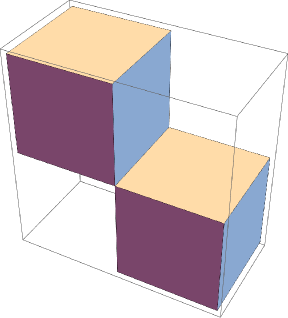
Keller (Keller1987, ) obtained this result as well, by noting that for 2D chessboards the current density in the less conductive domains decreases to the extent that current flow between the more conductive domains occurs mainly at the touching corners of those domains. For 3D chessboards, the current flow between the more conductive domains is concentrated at the touching edges of those domains. See Fig. 2 for an illustration of this geometry. Considering that $\sigma_{2D}=\left(\alpha\,\beta\right)^{1/2}$ even as $\beta/\alpha\rightarrow\infty$, the conductance at the edges of the higher-conductivity 3D domains is taken to be $\left(\alpha\,\beta\right)^{1/2}$. Then the factor of $2$ in Eq. (20) is obtained by accounting for the physical dimensions and 3D arrangement of the cubic domains.

Figure 2: For 3D chessboards with high contrast $\beta/\alpha$, the current flow between adjacent $\beta$-domains (the opaque cubes) occurs mainly at the “touching” edges of those domains.

Note that Eq. (18) gives the lower bound (LB)

$$\sigma_{dD}^{(\mathrm{LB)}}\sim\left(d-1\right)^{1/2}\left(\alpha\,\beta\right)^{1/2}$$ (21)

for a $d$-dimensional chessboard when the ratio $\beta/\alpha$ is very near infinity.

In comparison, Eq. (13) shows the behavior

$$\sigma_{dD}\sim\left(\frac{1}{2}\right)^{1-2/d}\alpha^{1/d}\,\beta^{1-1/d}$$ (22)

for a $d$-dimensional chessboard when the ratio $\beta/\alpha$ is very near infinity. Note that $\sigma_{3D}$ increases faster than does $\sigma_{2D}$ as $\beta\rightarrow\infty$, and $\sigma_{3D}$ declines more slowly than does $\sigma_{2D}$ as $\alpha\rightarrow 0$. This behavior is a consequence of the condition that $\sigma_{3D}>\sigma_{2D}$ when $\alpha\neq\beta$.

Kim (Kim2004, ) calculated several conductivity values for the 3D chessboard, using a Brownian motion simulation method in which walkers move according to first-passage-time equations. This numerical approach was developed by Kim and Torquato (Kim=000026Torq1990, ) and Torquato et al. (Torq=0000261999, ), and subsequently made more efficient by Kim (Kim2003, ).

Jylhä and Sihvola (Jyl=000026Sih2006, ) calculated several effective conductivity values pertinent to the 3D chessboard by use of a finite element code. Eight cubic domains comprising the “unit cell” of the chessboard contained about 274 000 elements. The mesh was sixteen times denser near the domain boundaries (faces), and a hundred times denser near the edges of the domains, than far from the boundaries. The applied electric field was normal to two opposing faces of the unit cell, and was forced to be tangental at the other four faces.

Note that these boundary conditions actually produce the effective conductivity $\sigma^{\prime}_{3D}$ of a block of eight contiguous domains sharing one corner, isolated from the rest of the (infinite) chessboard. Thus $\sigma^{\prime}_{3D}$ is the effective conductivity of a 3D array of these blocks. The current flow through this multi-block structure (in response to a potential difference across the structure) is less tortuous than the corresponding current flow through an actual 3D chessboard, so indicating $\sigma^{\prime}_{3D}>\sigma_{3D}$ for $\alpha\neq\beta$. In fact this block model provides a useful upper bound for $\sigma{}_{3D}$.

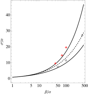
Figure 3 presents these analytical and numerical results for the 3D chessboard. The upper curve is a plot of Eq. (13),

$$\frac{\sigma_{3D}}{\alpha}=\frac{1+r}{2}\left[\frac{4\,r}{\left(1+r\right)^{2}}\right]^{1/3}$$ (23)

where $r=\beta/\alpha\geq 1$. The middle (dashed) curve is the corresponding plot of the bound Eq. (18): values for $\sigma_{3D}/\alpha$ should lie above it. The lower curve is a plot of $\sigma_{2D}/\alpha=\left(\beta/\alpha\right)^{1/2}$, for comparison to the other curves. The three points indicated by crosses (+), for $\beta/\alpha$ equal to $40,70,100$, are taken from Fig. 4 of Ref. (Jyl=000026Sih2006, ). The three points indicated by open circles (o), for $\beta/\alpha$ equal to $50,100,400$, are taken from Fig. 5 of Ref. (Kim2004, ).

Figure 3: Three curves showing (top to bottom) the derived Eq. (13) for $\sigma_{3D}$, the lower bound Eq. (18) for $\sigma_{3D}$, and $\sigma_{2D}$, for values $\beta/\alpha\geq 1$. The upper ($+$) and lower (o) sets of calculated points are taken from Ref. (Jyl=000026Sih2006, ) and Ref. (Kim2004, ), respectively.

V concluding remarks

The formula for $D_{w}^{(dD)}$ given by Eq. (7), and then Eq. (12), incorporates the symmetries and characteristics of the chessboard morphology in all dimensions. This is achieved by its expression as an exponential function, where the dimensional dependence resides in the exponent. In addition, this formulation satisfies the bound given by Eq. (15).

Future numerical work on the chessboard problem should focus on obtaining defensible bounds for $\sigma_{3D}$. These will support or disallow the analytic expression for $\sigma_{dD}$ given by Eq. (13).

Another two-component structure that occurs in all dimensions appears when $\alpha$ and $\beta$ sites are distributed randomly in the proportions $p_{c}$ and $\left(1-p_{c}\right)$, respectively. The fraction $p_{c}$ is the percolation threshold in the $d$-dimensional system. Thus $D_{w}^{(dD)}=0$ when $\beta=0$, and $D_{w}^{(dD)}=1$ when $\beta=\alpha$. The simplest expression for $D_{w}^{(dD)}$ is then

$$D_{w}^{(dD)}=\frac{\sigma_{dD}}{\left\langle\sigma(\mathbf{r})\right\rangle}=\frac{r^{u}}{p_{c}+\left(1-p_{c}\right)r}$$ (24)

where $r\equiv\beta/\alpha\leq 1$, and the value of the exponent $u$ depends on the dimension. In fact the effective conductivities of these $d$-dimensional systems do have the form

$$\sigma\left(p_{c},1;(1-p_{c}),r\right)=r^{u}$$ (25)

with $r\leq 1$. The exponents $u_{2D}=\nicefrac{{1}}{{2}}$ [CVSperc, ,Straley, ] and $u_{3D}=\nicefrac{{3}}{{4}}$ (CVSperc, ).