Entanglement Entropy of Fermions from Wigner Functions: Excited States and Open Quantum Systems

Abstract

We formulate a new “Wigner characteristics” based method to calculate entanglement entropies of subsystems of Fermions using Keldysh field theory. This bypasses the requirements of working with complicated manifolds for calculating Rényi entropies for many body systems. We provide an exact analytic formula for Rényi and von-Neumann entanglement entropies of non-interacting open quantum systems, which are initialised in arbitrary Fock states. We use this formalism to look at entanglement entropies of momentum Fock states of one-dimensional Fermions. We show that the entanglement entropy of a Fock state can scale either logarithmically or linearly with subsystem size, depending on whether the number of discontinuities in the momentum distribution is smaller or larger than the subsystem size. This classification of states in terms number of blocks of occupied momenta allows us to analytically estimate the number of critical and non-critical Fock states for a particular subsystem size. We also use this formalism to describe entanglement dynamics of an open quantum system starting with a single domain wall at the center of the system. Using entanglement entropy and mutual information, we understand the dynamics in terms of coherent motion of the domain wall wavefronts, creation and annihilation of domain walls and incoherent exchange of particles with the bath.

I Introduction

In a many body system, the erasure of information shows up as a classical probability in the description of the system. For quantum systems, if one starts from a generic pure quantum state and traces out some degrees of freedom, the description requires a “reduced” density matrix which allows quantum probability amplitudes and classical probabilities to co-exist in a single formalismHorodecki et al. (2009). Entanglement entropies (like Von-Neumann and Rényi entropies) are corresponding entropy measures of this resulting classical probability distribution, with the entanglement eigenvalues (the eigenvalues of the density matrix) giving the classical probability of finding the corresponding eigenstate in the ensemble. In this sense, entanglement entropies measure how much classical information is required to compensate for the loss of knowledge due to tracing over degrees of freedom.

Entanglement has been extensively studied in the context of quantum information and computation Nielsen and Chuang (2010), and in recent years, it has proved to be useful in many body physics as wellAmico et al. (2008). In particular, the scaling of bipartite entanglement entropy with subsystem size in ground statesEisert et al. (2010) has been used to detect topological phasesJiang et al. (2012); Kitaev and Preskill (2006); Grover et al. (2011) and quantum phase transitions Vidal et al. (2003). More recently, finite energy density eigenstates have also been shown to exhibit some universal scaling of entanglement entropy(EE) Vidmar et al. (2017); Hackl et al. (2019); Lu and Grover (2019a). Recently, entanglement entropy of many body systems have been measured experimentallyIslam et al. (2015); Lukin et al. (2019), although the system sizes are not in the thermodynamic limit. However, theoretical understanding of the same is comparatively still limited and efficient computational methods capable of accessing large system sizes are restricted to non-interacting theoriesPeschel (2003) or special integrable models in one dimension.

There have been three main approaches to calculating bipartite entanglement entropy of Fermionic quantum states: (1) Conformal Field Theory based approaches, which have yielded strong and crisp analytic predictions for size dependence of entanglement entropies in critical theories  Calabrese and Cardy (2009); Swingle (2012); Fradkin and Moore (2006) (2) Operator based approaches, which are confined to non-interacting systems, but have yielded exact answers Peschel (2003); Peschel and Eisler (2009) and (3) Field theory based approaches, which maps the problem to calculating partition function of the system on a Riemann surface with replicated sheets, with complicated boundary conditions Casini and Huerta (2009); Gioev and Klich (2006); Metlitski et al. (2009); Whitsitt et al. (2017) . There have of course been numerical approaches, which try to construct the state in the large dimensional Hilbert space either exactly (exact diagonalization)  Yu et al. (2016); Abanin et al. (2019); Samanta et al. (2020) or in approximate ways ( DMRG  Hastings et al. (2010); Grover (2013), Tensor Networks He et al. (2018)), and then work out the entanglement entropy by constructing a Schmidt decomposition of the state. With improvement of strategies to construct these states, this approach has yielded a wealth of information about structure of entanglement entropy of states. The numerical methods are less restricted than analytic ones in terms of applicability, but suffer from the problems of dealing with large Hilbert spaces.

In a recent paper, Chakraborty and Sensarma  Chakraborty and Sensarma (2018a) showed that Wigner characteristic functions for density matrices of bosonic many body systems are equivalent to partition functions in presence of time-localized sources (i.e. a delta function kick). The formalism can be adapted in a straightforward way to reduced density matrices by restricting the sources to the subregion where the reduced density matrix is supported. Combined with well known relations between Wigner functions and Rényi entropies of bosonic density matrices, this allowed a calculation of Rényi entropies of subsystems, which only involved correlation functions of the original model without any complicated Riemann surfaces. In this paper, we use similar ideas, combined with construction of “distribution functions” for Fermions by Glauber and Cahill Cahill and Glauber (1999), to show that one can construct Keldysh partition functions of the fermionic systems with time localized sources living on a subregion. One can use these Grassmann valued characteristic functions and integrate over the sources to obtain the Rényi entropies of arbitrary order, and hence von-Neumann entropy for a system of Fermions, both in and out of equilibrium. This part of the formalism was also developed independently by Haldar, Bera and Banerjee, who then went on to apply it to SYK models Haldar et al. (2020).

In this paper, we focus our attention on the application of this formalism to non equilibrium dynamics of Fermions in both open and closed quantum systems, starting from arbitrary initial conditions. A key result of this paper is that we obtain an exact analytic formula for the entanglement entropy of an open quantum system of Fermions whose dynamics start from an arbitrary initial Fock state. To our knowledge, this is the first time such a formula has been derived for open quantum dynamics with arbitrary initial conditions.

While a large amount of work has gone into understanding the entanglement properties of ground states of Fermions Eisert et al. (2010), the excited states have received relatively less analytic attention. Early work in this direction by Alba et. al  Alba et al. (2009) on entanglement entropy of excited states of $XY$ model showed the presence of “critical” states, whose entanglement entropy varied logarithmically with the size of the subsystem. Later works by Ares et.al Ares et al. (2014), Storms et al. Storms and Singh (2014), and more recently the works of Vidmar et al. Vidmar et al. (2017); Hackl et al. (2019), Carrasco et al. Carrasco et al. (2017), Jafarizadeh et al. Jafarizadeh and Rajabpour (2019), and Lu et al. Lu and Grover (2019b) have revived interest in the entanglement entropy of Fock states of Fermions We apply our exact formula to study the entanglement entropy of arbitrary momentum Fock states of spinless Fermions in one dimension. Here, our main results are: (i) For studying the behaviour of entanglement entropy, it is useful to classify Fock states in terms of number of blocks of occupied momenta in that state. This is similar to the classification proposed by Alba and Calabrese Alba et al. (2009) (ii) The entanglement entropy of a given Fock state scales logarithmically (“critical” behaviour) with the subsystem size if the subsystem size is much larger than the number of blocks of occupied momenta (or number of discontinuities in the momentum distribution) of the Fock state. The entropy scales linearly (“non-critical” behaviour) with the subsystem size when the number of discontinuities is much larger than the subsystem size. Thus Fock states are neither critical or non-critical by themselves, the same Fock state can appear critical or non-critical depending on the range of subsystem sizes one is probing. (iii) For a given subsystem size, we obtain an analytic estimate of the number of critical states in terms of the density of Fermions.

Entanglement dynamics in open quantum systems have been studied within the master equation approach Benatti et al. (2010) and quantum trajectory approach Nha and Carmichael (2004) , but they have been restricted to systems with $2$ or few qubitsAolita et al. (2015). A general analytic treatment of entanglement dynamics of many body systems starting from different initial conditions has been missing in the literature. Our exact formula fills this void for non-interacting Fermionic systems. Using this, we study the dynamics of an open quantum system of one dimensional spinless Fermions connected to a bath. We initialize this system in a Fock state with a density profile where the left half of the lattice is occupied and the right half is empty, creating a domain wall in the chain. We measure the time evolution of entanglement entropy of subsystems of different sizes placed at different locations in the system. We also look at the mutual information between the different components of a subsystem to see how they are entangled between themselves. We find that the dynamics of entanglement can be understood in terms three different processes: (i) an incoherent exchange of particles with the bath, which leads to a background evolution of entanglement, which does not depend on the location of the subsystem. (ii) A coherent wave of domain wall propagating and reflecting off the boundaries of the system, which leads to sharp jumps in entanglement entropy. These jumps occur at different times for subsystems at different locations, revealing the propagation and reflection of the wave. The coherent wave is damped by dissipation from the bath, and (iii) Local Rabi oscillations between nearest neighbours which also lead to splitting and merging of domains. This process leaves its imprint in the form of oscillations superposed on an overall background. We show that once the coherent wave hits the subsystem there is a sharp increase in the mutual information between the components of the subsystem, showing that they are getting entangled in the process. Finally, as the system evolves from a pure quantum state to a density matrix characterized by a thermal ensemble in the long time limit, we focus on the additional entropy density (entropy per site) of a subsystem vis-a-vis the full system, which represents the entropy of information loss due to tracing of degrees of freedom. We show that while the time evolution of entanglement entropy of larger subsystems closely follow that of the full system, the effects of the quantum processes can be cleanly demonstrated in the evolution of the excess entropy density.

We now provide a roadmap for the different sections of the paper: (i) In Section II, we define the Grassmann valued “Wigner characteristic function” of a fermionic density matrix, previously discussed by Glauber and Cahill Cahill and Glauber (1999), and show how one can relate integrals (over Grassmann valued arguments) of these functions to Rényi entropies of different orders. (ii) In Section III, we show how the Keldysh partition function of a Fermionic system with particular arrangement of sources is equal to the Wigner characteristic function of the reduced density matrix of a subsystem. (iii) In Section IV, we will extend this formalism to the case of non-equilibrium dynamics starting from arbitrary initial states. (iv) In section V, we derive an exact analytic formula for Rényi and von Neumann entropies of a subsystem of a open quantum system of non-interacting Fermions starting from an arbitrary Fock state. (vi) In section VI, we will focus our attention on arbitrary momentum Fock states and show that they can exibit linear or logarithmic scaling of entanglement entropy with subsystem size, depending the range of subsystem sizes one is probing. (vii) In section VII, we will study the evolution of entanglement entropy and mutual information in an open quantum system of one dimensional Fermions starting from a state with one half occupied and the other half empty.

II Wigner Functions and Entanglement Entropy of Fermions

We will study a system of $N$ spinless Fermions on a lattice with $V$ sites and calculate Rényi and von Neumann entropies of a subsystem $A$ with $V_{A}$ sites. We will consider a complete single particle basis $i$ with $V$ distinct values, and corresponding creation/annihilation operators $c^{\dagger}_{i}$ ( $c_{i}$). The Fermionic coherent states, defined by $|\bm{\zeta},\bm{\bar{\zeta}}\rangle:=\hat{D}(\bm{\zeta},\bm{\bar{\zeta}})|0\rangle$, are labelled by tuples of Grassman variables $\bm{\zeta}=(\zeta_{1},\zeta_{2},\mathellipsis,\zeta_{M})^{T}$ and $\bm{\bar{\zeta}}=(\bar{\zeta}_{1},\bar{\zeta}_{2},\mathellipsis,\bar{\zeta}_{M})$, where $M$ is the number of modes, $|0\rangle$ is the vacuum state, and the displacement operator is given by

$$\hat{D}(\bm{\zeta},\bm{\bar{\zeta}}):=\mathrm{e}^{\sum_{i}c^{\dagger}_{i}\zeta_{i}-\bar{\zeta}_{i}c_{i}}=\prod_{i}[1+\zeta_{i}c^{\dagger}_{i}-\bar{\zeta}_{i}c^{\dagger}_{i}-\bar{\zeta}_{i}\zeta_{i}(1/2-c^{\dagger}_{i}c_{i})]$$ (1)

These operators can be combined using

$$\hat{D}(\bm{\zeta},\bm{\bar{\zeta}})\hat{D}(\bm{\eta},\bm{\bar{\eta}})=\hat{D}(\bm{\zeta}+\bm{\eta},\bm{\bar{\zeta}}+\bm{\bar{\eta}})\,\mathrm{e}^{\frac{1}{2}\left(\bm{\bar{\eta}}\cdot\bm{\zeta}-\bm{\bar{\zeta}}\cdot\bm{\eta}\right)}.$$ (2)

To construct various “quasi-distribution functions”, in a vein similar to the Wigner distribution for BosonsCahill and Glauber (1969), it is useful to introduce another operator $\hat{E}(\bm{\zeta},\bm{\bar{\zeta}})$ where

$$\hat{E}(\bm{\zeta},\bm{\bar{\zeta}})=\prod_{i}(1-2c^{\dagger}_{i}c_{i})\hat{D}(\bm{\zeta},\bm{\bar{\zeta}})=\mathrm{e}^{i\pi\hat{N}_{tot}}\hat{D}(\bm{\zeta},\bm{\bar{\zeta}}).$$ (3)

$\hat{N}_{tot}$ is the total Fermion number operator. $\hat{E}$ is thus related to $\hat{D}$ by the fermion parity operator. This operator was first introduced by Cahill and Glauber  Cahill and Glauber (1999), although our definition differs from theirs by a sign of the arguments.

In this case, one can easily show that the delta function over Grassmans can be represented as

$$\delta(\bm{\zeta}-\bm{\eta}):=\prod_{i}(\zeta_{i}-\eta_{i})(\bar{\zeta}_{i}-\bar{\eta}_{i})=\mathrm{Tr}\left[\hat{D}(\bm{\zeta},\bm{\bar{\zeta}})\hat{E}(\bm{\eta},\bm{\bar{\eta}})\right]$$ (4)

where $\eta_{i}$ and $\bar{\eta}_{i}$ are Grassman variables. We note that any operator in the Fermionic Fock space, which preserves total Fermion parity, can be expanded in terms of either $\hat{D}$ or $\hat{E}$ as

$$\hat{F} = \int\mathcal{D}\left[\bm{\zeta},\bm{\bar{\zeta}}\right]f_{D}(\bm{\zeta},\bm{\bar{\zeta}})\hat{D}(\bm{\zeta},\bm{\bar{\zeta}})$$ (5)

$$= \int\mathcal{D}\left[\bm{\zeta},\bm{\bar{\zeta}}\right]f_{E}(\bm{\zeta},\bm{\bar{\zeta}})\hat{E}(\bm{\zeta},\bm{\bar{\zeta}})$$

where $\mathcal{D}\left[\bm{\zeta},\bm{\bar{\zeta}}\right]:=\prod_{i}\mathrm{d}\bar{\zeta}_{i}\mathrm{d}\zeta_{i}$ and

$$f_{D}(\bm{\zeta},\bm{\bar{\zeta}}) =\mathrm{Tr}\left[\hat{F}\hat{E}(\bm{\zeta},\bm{\bar{\zeta}})\right]$$

$$f_{E}(\bm{\zeta},\bm{\bar{\zeta}}) =\mathrm{Tr}\left[\hat{D}(\bm{\zeta},\bm{\bar{\zeta}})\hat{F}\right]$$ (6)

As a consequence of this, one can expand $\hat{E}$ in terms of $\hat{D}$,

$$\hat{E}(\bm{\zeta},\bm{\bar{\zeta}})=2^{M}\int\mathcal{D}\left[\bm{\eta},\bm{\bar{\eta}}\right]\hat{D}(\bm{\eta},\bm{\bar{\eta}})\mathrm{e}^{\frac{1}{2}\sum_{i}\bar{\zeta}_{i}\eta_{i}-\bar{\eta}_{i}\zeta_{i}}$$ (7)

One can now define the equivalent of the Wigner characteristic function for fermions,

$$\chi_{D}(\bm{\zeta},\bm{\bar{\zeta}}) =\rho_{E}(\bm{\zeta},\bm{\bar{\zeta}})=\mathrm{Tr}\left[\hat{\rho}\hat{D}(\bm{\zeta},\bm{\bar{\zeta}})\right]$$ (8)

$$\chi_{E}(\bm{\zeta},\bm{\bar{\zeta}}) =\rho_{D}(\bm{\zeta},\bm{\bar{\zeta}})=\mathrm{Tr}\left[\hat{\rho}\hat{E}(\bm{\zeta},\bm{\bar{\zeta}})\right]$$

$$=2^{M}\int\mathcal{D}\left[\bm{\eta},\bm{\bar{\eta}}\right]\chi_{D}(\bm{\eta},\bm{\bar{\eta}})\mathrm{e}^{\frac{1}{2}\sum_{i}\bar{\zeta}_{i}\eta_{i}-\bar{\eta}_{i}\zeta_{i}}$$

where $\hat{\rho}$ is the density matrix of the system in a $2^{M}$ dimensional Hilbert space. For a reduced density matrix of a subsystem of $V_{A}$ sites, $M=V_{A}$. All operator expectations can be written in terms of $\chi_{D}$ and we will later see that $\chi_{D}$ can be calculated within a path-integral/field theoretic approach.

Using the expansions, Eq. 5 and Eq. 6, together with the identity Eq. 4, the expectation of parity preserving operators are given by

$$\langle\hat{F}\rangle=\mathrm{Tr}\left[\hat{F}\hat{\rho}\right]=\int{\cal D}[\bm{\zeta},\bm{\bar{\zeta}}]~{}f_{D}(\bm{\zeta},\bm{\bar{\zeta}})~{}\chi_{D}(\bm{\zeta},\bm{\bar{\zeta}})$$ (9)

The second Rényi entropy, $S^{(2)}=-\ln\mathrm{Tr}\left[\hat{\rho}_{r}^{2}\right]$, is

$$S^{(2)}=-\ln\left[2^{V_{A}}\int\mathcal{D}\left[\bm{\zeta},\bm{\bar{\zeta}}\right]\mathcal{D}\left[\bm{\eta},\bm{\bar{\eta}}\right]\hskip 1.0pt\chi^{r}_{D}(\bm{\zeta},\bm{\bar{\zeta}})\,\chi^{r}_{D}(\bm{\eta},\bm{\bar{\eta}})\,\mathrm{e}^{\frac{1}{2}\sum^{{}^{\prime}}_{x}\bar{\zeta}_{x}\eta_{x}-\bar{\eta}_{x}\zeta_{x}}\right]$$ (10)

where $\hat{\rho}_{r}$ is the reduced density matrix. Here the ^′ in the summation indicates that the spatial index $x$ runs only over the subsystem $A$. Note that in case of continuum theories, the sum will be replaced by appropriate integrals. The above result can be generalized to the trace of $n$ operators to get the relation between the $n^{th}$ order Rényi entropy $S^{(n)}$ and the Wigner characteristic of the reduced density matrix

$$\begin{split}S^{(n)}=\frac{1}{1-n}\ln\left[2^{({n-1})V_{A}}\int\prod_{i=1}^{n-1}\mathcal{D}[\bm{\zeta}^{(i)},\bm{\bar{\zeta}}^{(i)}]\mathcal{D}[\bm{\eta}^{(i)},\bm{\bar{\eta}}^{(i)}]\prod_{i=1}^{n-1}\chi^{r}_{D}[\bm{\eta}^{(i)},\bm{\bar{\eta}}^{(i)}]~{}\chi^{r}_{D}\left[{\small\sum}\bm{\zeta}^{(i)},{\small\sum}\bm{\bar{\zeta}}^{(i)}\right]\right.\\ \left.\exp\frac{1}{2}\left({\sum_{i}\bm{\bar{\zeta}}^{(i)}\!\cdot\bm{\eta}^{(i)}-\bm{\bar{\eta}}^{(i)}\!\cdot\bm{\zeta}^{(i)}+\sum_{i>j}\bm{\bar{\zeta}}^{(i)}\!\cdot\bm{\zeta}^{(j)}-\bm{\bar{\zeta}}^{(j)}\!\cdot\bm{\zeta}^{(i)}}\right)\right]\end{split}$$ (11)

We note that if all the Renyi entropies are analytically known, the von Neumann entropy can be calculated by analytic continuation $S_{vN}:=\lim_{n\rightarrow 1}S^{(n)}$. Having related all the Rényi entanglement entropies of a subsystem of fermions to the Wigner characteristic function of the reduced density matrix $\chi^{r}_{D}$, we now focus our attention on methods to compute this function. In the next section, we will relate $\chi_{D}^{r}$ to a Schwinger Keldysh partition function of the fermionic system in presence of a particular set of sources.

III Keldysh Field Theory and Wigner Characteristic Function

Schwinger Keldysh field theories can describe quantum dynamics of both open and closed quantum many body systems out of thermal equilibrium. The key idea is to consider the time evolution of the density matrix, $\hat{\rho}(t)=\hat{U}(t,0)\hat{\rho}(0)\hat{U}^{\dagger}(t,0)$ and expand the forward time evolution operator $U$ in a path/functional integral with Grassmann fields $\psi_{+}(x,t)$ and $\bar{\psi}_{+}(x,t)$. The backward time evolution operator has a similar expansion in terms of $\psi_{-}(x,t)$ and $\bar{\psi}_{-}(x,t)$. This leads to a field theory with two copies of fields at each space time points.

Observables $O(t)=\mathrm{Tr}\left[\hat{O}\hat{\rho}(t)\right]/tr{\hat{\rho}(t)}$ are usually obtained in the field theoretic formalism by coupling sources to the fields, $J_{\pm}(x,t)$ coupling to $\bar{\psi}_{\pm}(x,t)$ and $\bar{J}_{\pm}(x,t)$ coupling to $\psi_{\pm}(x,t)$, and taking derivatives with respect to these sources, before setting the sources to zero. For time local observables, the standard practice is to take a symmetric linear combination of placing the operator on the $+$ and $-$ contour; i.e. $O(t)=[O_{+}(t)+O_{-}(t)]/2$.

It was first shown in Ref Chakraborty and Sensarma, 2018a, that the expectation of the displacement operator for a system of Bosons is equivalent to the Keldysh partition function in presence of a particular set of sources. We follow similar algebra to show that this holds for Fermionic Wigner characteristics as well. The key innovation in this derivation is to consider

$$\chi_{D}(\bm{\zeta},\bm{\bar{\zeta}},t)=\frac{\mathrm{Tr}\left[\hat{U}(\infty,t)\hat{D}^{1/2}(\bm{\zeta}/2,\bar{\bm{\zeta}}/2)\hat{U}(t,0)\hat{\rho}_{0}\hat{U}^{\dagger}(t,0)\hat{D}^{1/2}(\bm{\zeta}/2,\bar{\bm{\zeta}}/2)\hat{U}^{\dagger}(\infty,t)\right]}{\mathrm{Tr}\left[\hat{U}(\infty,0)\hat{\rho}_{0}\hat{U}^{\dagger}(\infty,0)\right]}$$ (12)

or $D\sim D^{1/2}_{+}D^{1/2}_{-}$, i.e. a multiplicative rather than a linear decomposition. We note that $\hat{D}^{1/2}$ is not a normal ordered operator. However, considering the anti-commutation of the Grassman fields, it can be shown that the insertion of $\hat{D}^{1/2}$ on the $\pm$ contour is equivalent to turning on a source $J_{\pm}(x,\tau)=\pm\iota\zeta_{x}\delta(\tau-t)$. We note that the change of sign between the sources on the $+$ and $-$ contour is due to the fact that the action on the $-$ contour has a $-$ sign relative to the action on the $+$ contour in the Keldysh formalism. Thus we can identify

$$\chi_{D}(\bm{\zeta},\bm{\bar{\zeta}},t)=Z\left[J_{\pm}(x,\tau)=\pm\iota\zeta_{x}\delta(\tau-t),\bar{J}_{\pm}(x,\tau)=\mp\iota\bar{\zeta}_{x}\delta(\tau-t)\right]$$ (13)

i.e. Wigner characteristic is the partition function with the above set of sources. For fermionic systems, it is useful to work with symmetric and antisymmetric combinations of the fields,

$$\psi_{1}(x,t) =[\psi_{+}(x,t)+\psi_{-}(x,t)]/\sqrt{2} \quad\psi_{2}(x,t) =[\psi_{+}(x,t)-\psi_{-}(x,t)]/\sqrt{2}$$ (14)

$$\bar{\psi}_{1}(x,t) =[\bar{\psi}_{+}(x,t)-\bar{\psi}_{-}(x,t)]/\sqrt{2} \quad\bar{\psi}_{2}(x,t) =[\bar{\psi}_{+}(x,t)+\bar{\psi}_{-}(x,t)]/\sqrt{2}.$$

One can similarly define sources $J_{1}(x,t)=[J_{+}(x,t)+J_{-}(x,t)]/\sqrt{2}$, $J_{2}(x,t)=[J_{+}(x,t)-J_{-}(x,t)]/\sqrt{2}$, $\bar{J}_{1}(x,t)=[\bar{J}_{+}(x,t)-\bar{J}_{-}(x,t)]/\sqrt{2}$ and $\bar{J}_{2}(x,t)=[\bar{J}_{+}(x,t)+\bar{J}_{-}(x,t)]/\sqrt{2}$, which couple to the respective rotated fields. If one considers the source pattern required for evaluating the Wigner characteristic in this Keldysh rotated basis, one finds that $J_{1}(x,\tau)=\bar{J}_{2}(x,\tau)=0$, with $\bar{J}_{1}(x,\tau)=-\frac{\iota}{\sqrt{2}}\bar{\zeta}_{x}\delta(t-\tau)$ and $J_{2}(x,\tau)=\frac{\iota}{\sqrt{2}}\zeta_{x}\delta(t-\tau)$. This leads to the final result

$$\chi_{D}(\bm{\zeta},\bm{\bar{\zeta}},t)=Z\left[J_{1}(x,\tau)=0,\bar{J}_{1}(x,\tau)=-\frac{\iota}{\sqrt{2}}\bar{\zeta}_{x}\delta(t-\tau),J_{2}(x,\tau)=\frac{\iota}{\sqrt{2}}\zeta_{x}\delta(t-\tau),\bar{J}_{2}(x,\tau)=0\right]$$ (15)

Note that the above equation is true for general interacting open or closed systems of Fermions.

To calculate Rényi entropies, one divides the system into subsystems $A$ and $B$ and traces the density matrix over degrees of freedom residing in $B$ to obtain a reduced density matrix. One then considers traces of products of such reduced density matrices. The standard field theoretic way of calculating this is to consider a field theory on a replicated manifold with complicated boundary conditions on the fields in the region $A$. In our formalism, the calculation of partition function naturally traces over degrees of freedom. To calculate the Wigner characteristic of the reduced density matrix (instead of the full density matrix), we simply need to restrict the sources to be nonzero in the region $A$ rather than the whole system. This makes our formalism ideally suited for calculating entanglement entropies of subsystem of Fermions.

We note that the standard Keldysh Field theory can treat non-equilibrium dynamics of the system (including coupling to baths), provided the initial state is in thermal equilibrium. We will deal with the case of arbitrary initial conditions in the next section. For thermal initial states, the gaussian action for a non-interacting system can be written as

$$S=\int dt\int dt^{\prime}\sum_{x,x^{\prime}}\psi^{\dagger}(x,t)G^{-1}(x,t;x^{\prime},t^{\prime})\psi(x^{\prime},t^{\prime})$$ (16)

Here $\psi^{\dagger}(x,t)=[\bar{\psi}_{1}(x,t),\bar{\psi}_{2}(x,t)]$. The inverse propagator $G^{-1}$ and the one particle Green’s functions $G$ have the structure

$$\hat{G}^{-1}=\left[\begin{array}[]{cc}(\hat{G}^{R})^{-1}&(\hat{G}^{-1})^{K}\\ 0&(\hat{G}^{A})^{-1}\end{array}\right]~{}~{}~{}~{}~{}\hat{G}=\left[\begin{array}[]{cc}\hat{G}^{R}&\hat{G}^{K}\\ 0&\hat{G}^{A}\end{array}\right]$$ (17)

where $\hat{G}^{R(A)}$ is the retarded (advanced) one particle Green’s function, and $\hat{G}^{K}$ is the Keldysh Green’s function . The equal time Keldysh Green’s function is related to the physical one particle correlators in the system. In this case, the functional integrals over the fermion fields can be carried out to compute the Wigner characteristic of the reduced density matrix

$$\chi^{r}_{D}(\bm{\zeta},\bm{\bar{\zeta}},t)=\mathrm{e}^{-\frac{1}{2}\sum^{{}^{\prime}}_{xx^{\prime}}\bar{\zeta}_{x}[\iota G^{K}(x,t;x^{\prime},t)]\zeta_{x^{\prime}}}$$ (18)

where once again $x$ and $x^{\prime}$ are restricted to the subregion $A$, and we have used the fact that partition function of a Keldysh field theory in absence of external sources is $1$ (this takes care of a factor of $\det\hat{G}^{-1}$ coming from the functional integrals). We will not comment on the particular form of $\hat{G}^{K}$ here, except reminding the readers that $\hat{G}^{K}$ is an anti-hermitian matrix in the space-time indices. This form of $\chi_{D}$ can then be used to calculate the second Rényi entropy

$$S^{(2)}(t)=-\ln\left[2^{L_{A}}\int{\cal D}[\bm{\zeta},\bm{\bar{\zeta}}]{\cal D}[\bm{\eta},\bm{\bar{\eta}}]~{}\mathrm{e}^{-\frac{1}{2}\sum^{{}^{\prime}}_{xx^{\prime}}(\bar{\zeta}_{x},\bar{\eta}_{x})\left(\begin{array}[]{cc}\iota G^{K}(x,t;x^{\prime},t)&-\delta_{x,x^{\prime}}\\ \delta_{x,x^{\prime}}&\iota G^{K}(x,t;x^{\prime},t)\end{array}\right)\left(\begin{array}[]{c}\zeta_{x^{\prime}}\\ \eta_{x^{\prime}}\end{array}\right)}\right]=-\mathrm{Tr}\left[\ln[\hat{1}+(\iota\hat{G}^{K}(t))^{2}]\right]$$ (19)

where the matrix $\hat{G}^{K}(t)=G^{K}(x,t;x^{\prime},t)$ is in the space of spatial co-ordinates running over subregion $A$. One can in fact write down a general expression for the $n^{th}$ order Rényi entropy of the system in terms of the Keldysh Green’s function of the system

$$S^{(n)}(t)=\frac{1}{1-n}\mathrm{Tr}\left[\ln\left[\left(\frac{\hat{1}-\iota\hat{G}^{K}(t)}{2}\right)^{n}+\left(\frac{\hat{1}+\iota\hat{G}^{K}(t)}{2}\right)^{n}\right]\right]$$ (20)

We can analytically continue the expression for $S^{(n)}$ to $n\to 1$ to get

$$S_{\text{vN}}=-\mathrm{tr}\left[\ln\left[\left(\frac{\hat{1}-\iota\hat{G}^{K}(t)}{2}\right)\ln\left(\frac{\hat{1}-\iota\hat{G}^{K}(t)}{2}\right)+\left(\frac{\hat{1}+\iota\hat{G}^{K}(t)}{2}\right)\ln\left(\frac{\hat{1}+\iota\hat{G}^{K}(t)}{2}\right)\right]\right]$$ (21)

This recovers the well known formula of RefPeschel, 2003 with the role of the correlation matrix played by $({\hat{1}-\iota\hat{G}^{K}(t)})/{2}$

IV Arbitrary Initial conditions

A large class of interesting problems regarding dynamics of entanglement entropies require description of dynamics starting from non-thermal initial states; e.g. we may be interested in starting an open quantum system in a product state in real space (with zero Rényi entropy) and describe the growth of entanglement as the system thermalizes. While textbook Keldysh field theory requires a thermal initial state, recent developments Chakraborty et al. (2019) have provided a way to describe quantum dynamics of many body systems starting from arbitrary initial conditions.By focussing at the initial time, the formalism can be easily adapted to investigate the entanglement entropy of particular Fock states or density matrices.

Here we will briefly review the formalism of incorporating initial athermal states as applied to the calculation of the Wigner characteristicsChakraborty et al. (2019). Consider an initial density matrix of the form $\hat{\rho}_{0}=\sum_{\{n\}}c_{\{n\}}|\{n\}\rangle\langle\{n\}|$ where $|\{n\}\rangle=\otimes_{\alpha}|n_{\alpha}\rangle$ is the occupation number state, and $\alpha$ denotes a single particle basis state. Note that $\alpha$ does not need to be a spatial co-ordinate; this formalism will work for any complete one particle basis. In this case, we need to add to the original Keldysh action a bilinear source term at $t=0$, $\delta S(u)=\iota\sum_{\alpha}\psi^{\ast}_{1}(\alpha,0)\psi_{2}(\alpha,0)\frac{1-u_{\alpha}}{1+u_{\alpha}}$. One then calculates the Wigner characteristic in this theory by adding appropriate sources and calculating the partition function in presence of these sources,

$$\chi^{r}_{D}(\bm{\zeta},\bm{\bar{\zeta}},t|\bm{u})=Z\left[J_{1}(x,\tau)=0,\bar{J}_{1}(x,\tau)=-\frac{\iota}{\sqrt{2}}\bar{\zeta}_{x}\delta(t-\tau),J_{2}(x,\tau)=\frac{\iota}{\sqrt{2}}\zeta_{x}\delta(t-\tau),\bar{J}_{2}(x,\tau)=0,u\right]$$ (22)

The Wigner characteristic for the dynamics with the initial condition is then given by

$$\chi^{r}_{D}(\bm{\zeta},\bm{\bar{\zeta}},t,)={\cal L}(\partial_{u},\rho_{0}){\cal N}(\bm{u})\chi_{D}(\bm{\zeta},\bm{\bar{\zeta}},t|\bm{u})|_{u=0}$$ (23)

where ${\cal N}(u)=\prod_{\alpha}(1+u_{\alpha})$ and ${\cal L}=\sum_{\{n\}}c_{\{n\}}\prod_{\alpha\in\mathcal{A}}\partial_{u_{\alpha}}$. ${\mathcal{A}}$ is the set of occupied modes in $|\{n\}\rangle$. For the case of an initial pure Fock state, we get

$$\chi^{r}_{D}(\bm{\zeta},\bm{\bar{\zeta}},t)=\prod_{\alpha}[1+n_{\alpha}\partial_{u_{\alpha}}]\chi_{D}(\bm{\zeta},\bm{\bar{\zeta}},t|\bm{u})|_{u=0}$$ (24)

Let us understand the consequences of these equations in the case of a non-interacting theory (with coupling to baths). The Wigner characteristic in presence of the sources $u$ will be given by

$$\chi^{r}_{D}(\bm{\zeta},\bm{\bar{\zeta}},t|\bm{u})=\exp\left[{-\frac{1}{2}\sum_{x,x^{\prime}\in A}\bar{\zeta}_{x}[\iota G^{K}(x,t;x^{\prime},t|\bm{u})]\zeta_{x^{\prime}}}\right]$$ (25)

In this case, the Keldysh Green’s function in presence of the $u$ sources is given by

$$\iota G^{K}(x,t;x^{\prime},t^{\prime}|\bm{u})=\sum_{\alpha}G^{R}(x,t;\alpha,0)G^{A}(\alpha,0;x^{\prime},t^{\prime})\frac{1-u_{\alpha}}{1+u_{\alpha}}+\iota\int_{0}^{t}dt_{1}\int_{0}^{t^{\prime}}dt_{2}G^{R}(x,t;x_{1},t_{1})\Sigma^{K}(x_{1},t_{1};x_{2},t_{2})G^{A}(x_{2},t_{2};x^{\prime},t^{\prime})$$ (26)

where $\Sigma^{K}$ is the Keldysh self energy due to possible coupling to external baths. Note once again that $\alpha$ is not necessarily a spatial co-ordinate; it can for example denote momentum labels. The physical Keldysh Greens function $\mathcal{G}^{K}$ is given in terms of the $\bm{u}$ dependent ones as

$$\iota\mathcal{G}^{K}(x,t;x^{\prime},t^{\prime}) ={\cal L}(\partial_{u},\hat{\rho}_{0})[{\cal N}(\bm{u})\iota G^{K}(x,t;x^{\prime},t^{\prime}|\bm{u})]|_{\bm{u}=0}$$

$$=\prod_{\alpha}[1+n_{\alpha}\partial_{u_{\alpha}}]\iota G^{K}(x,t;x^{\prime},t^{\prime}|\bm{u})]|_{\bm{u}=0}$$ (27)

One can show from Eq.26 that

$$\iota\mathcal{G}^{K}(x,t;x^{\prime},t^{\prime})=\Gamma(x,x^{\prime},t)-2\Lambda(x,x^{\prime},t)$$ (28)

where we define the following quantities as

$$\Lambda^{\alpha}(x,x^{\prime},t) =-\frac{1}{2}\partial_{u_{\alpha}}[\iota G^{K}(x,t;x^{\prime},t|\bm{u})]|_{u=0}=G^{R}(x,t;\alpha,0)[G^{R}(x^{\prime},t;\alpha,0)]^{\ast}$$

$$\Lambda(x,x^{\prime},t) =\sum_{\alpha}n_{\alpha}\Lambda^{\alpha}(x,x^{\prime},t)$$ (29)

$$\Gamma(x,x^{\prime},t) =\iota G^{K}(x,t;x^{\prime},t|\bm{u}=0)=\sum_{\alpha}\Lambda^{\alpha}(x,x^{\prime},t)+\iota\int_{0}^{t}dt_{1}\int_{0}^{t^{\prime}}dt_{2}G^{R}(x,t;x_{1},t_{1})\Sigma^{K}(x_{1},t_{1};x_{2},t_{2})G^{A}(x_{2},t_{2};x^{\prime},t^{\prime})$$

The initial condition specification $\{n_{\alpha}\}$ is entirely incorporated in $\Lambda$ alone, whereas $\Gamma$ is independent of the initial conditions and is fully determined by the system dynamics.

In the next section, we will first integrate over the arguments of the Wigner characteristic functions and then evaluate these multiple derivatives exactly to present an analytic answer for Rényi entropies of different orders (as well as the Von-Neuman entanglement entropy) of subsystems of non-interacting open quantum systems of Fermions. To our knowledge, this is the first time such a general formula is being derived for open quantum systems. An alternative formulation, where the derivatives are first computed to get the Wigner characteristic and the integrations are performed afterwards, leads to a diagrammatic evaluation of entanglement entropies. This will be shown in Appendix  A.

V Exact Formula for Entanglement entropies of Open Quantum Systems

In this section we will work out in detail the exact formula for the second Rényi entanglement entropy of an open quantum system. We will also provide the final answers for the $n^{th}$ order Rényi entropy, and hence for the Von-Neumann entanglement entropy for the system. The detailed derivation for this will be presented in Appendix  B.

The second Rényi entropy of an open quantum system, starting from a particular initial Fock state is given by

$$\mathrm{e}^{-S^{(2)}}=\prod_{\alpha}[1+n_{\alpha}\partial_{u_{\alpha}}]\prod_{\alpha}[1+n_{\beta}\partial_{v_{\beta}}]2^{V_{A}}\left[\int{\cal D}[\bm{\zeta},\bm{\bar{\zeta}}]{\cal D}[\bm{\eta},\bm{\bar{\eta}}]~{}\mathrm{e}^{-\frac{1}{2}\sum^{{}^{\prime}}(\bar{\zeta}_{x},\bar{\eta_{x}})\left(\begin{array}[]{cc}\iota G^{K}(x,t;x^{\prime},t|\bm{u})&-\delta_{x,x^{\prime}}\\ \delta_{x,x^{\prime}}&\iota G^{K}(x,t;x^{\prime},t|\bm{v})\end{array}\right)\left(\begin{array}[]{c}\zeta_{x^{\prime}}\\ \eta_{x^{\prime}}\end{array}\right)}\right]$$ (30)

where $G^{K}(x,t;x^{\prime},t|\bm{u})$ is given by Eq. 26. The gaussian integrals can be performed easily to get

$$\mathrm{e}^{-S^{(2)}}=\prod_{\alpha}\left[1+n_{\alpha}\partial_{u_{\alpha}}\right]\prod_{\beta}\left[1+n_{\beta}\partial_{v_{\beta}}\right]\left.\left[\frac{1}{2^{V_{A}}}\det\left[\mathbb{M}\right]\right]\right|_{{\tiny\begin{array}[]{c}\bm{u}=0\\ \bm{v}=0\end{array}}}$$ (31)

where $\mathbb{M}$ is a $2V_{A}\times 2V_{A}$ matrix defined as

$$\mathbb{M}\equiv\left(\begin{array}[]{cc}\mathbb{U}(\bm{u})&\mathbb{V}(\bm{v})\end{array}\right):=\left(\begin{array}[]{cc}\iota\hat{G}^{K}(\bm{u})&-\hat{1}\\ \hat{1}&\iota\hat{G}^{K}(\bm{v})\end{array}\right)$$ (32)

$\mathbb{U}$ & $\mathbb{V}$ are $2V_{A}\times V_{A}$ matrices depending on only $\bm{u}=\{u_{\alpha}\}$ and $\bm{v}=\{v_{\beta}\}$ respectively, and we have suppressed the matrix indices of $G^{K}$ for notational convenience. It is clear that

$$\mathbb{M}(\bm{u}=0,\bm{v}=0)=\left(\begin{array}[]{cc}\hat{\Gamma}&-\hat{1}\\ \hat{1}&\hphantom{-}\hat{\Gamma}\end{array}\right)$$ (33)

Note that the $u_{\alpha}$ derivatives only act on $\mathbb{U}$ and similarly $\{\partial_{v_{\beta}}\}$ only act on $\mathbb{V}$. Hence we can treat them separately and focus solely on the action of $\prod_{\alpha}[1+n_{\alpha}\partial_{u_{\alpha}}]$ on $\det\mathbb{M}$ for the sake of illustration.

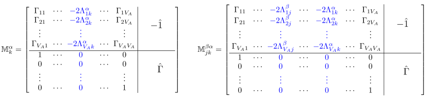
Figure 1: The matrix M obtained by taking u-derivatives of the determinant in Eq. 30 Note that the full answer for Rényi entropy is obtained by taking a sum of determinants of many such matrices. See text for details.

The first thing to note is that $\partial_{u_{\alpha}}\partial_{u_{\beta}}G^{K}(x,t;x^{\prime},t|\bm{u})=0$, i.e. there can only be a single derivative of a particular matrix element. Let us consider a single $u_{\alpha}$ derivative acting on $\text{det}~{}\mathbb{M}$. Consider a matrix where the matrix elements in all columns except the $x^{th}$ one ($x\leq V_{A}$) are same as $\mathbb{M}$, while the matrix elements in the $x^{th}$ column are replaced by their $u_{\alpha}$ derivatives. Let us call this matrix $\mathbb{M}^{\alpha}_{x}$. If we set $\bm{u}=\bm{v}=0$ in this matrix, we will replace the $x^{th}$ column by $\{-2\Lambda^{\alpha}(i,x)\}|_{i=1}^{V_{A}}$ on the top half and a $0$ vector in the bottom half. This matrix is shown in Fig 1. It is then easy to show that the derivative of the determinant is the sum of the determinant of these matrices, from $x=1$ to $x=V_{A}$

$$\partial_{u_{\alpha}}|\mathbb{M}|=\sum_{x=1}^{V_{A}}|\mathbb{M}^{\alpha}_{x}|$$ (34)

Here, for brevity we denote $|\ast|:=\det[\,\ast\,]$. One can take this argument forward to show that

$$\partial_{u_{\alpha}}\partial_{u_{\beta}}|\mathbb{M}|=\sum_{x_{1}\neq x_{2}}|\mathbb{M}^{\beta\alpha}_{x_{1}x_{2}}|$$ (35)

where $\mathbb{M}^{\beta\alpha}_{xx^{\prime}}$ is the matrix $\mathbb{M}$ with the $x_{1}^{th}$ column replaced by its $u_{\beta}$ derivative and the $x_{2}^{th}$ column replaced by its $u_{\alpha}$ derivative. For $(\bm{u},\bm{v})=0$, this matrix is shown in Fig 1. The $x_{1}^{th}$ column is replaced by $-2\Lambda_{\beta}(k,x_{1})$ and the $x_{2}^{th}$ column is replaced by $-2\Lambda^{\alpha}(k,x_{2})$. One can extend this construction for higher order derivatives to get

$$\prod_{\alpha}\left[1+n_{\alpha}\partial_{u_{\alpha}}\right]\lvert\mathbb{M}\rvert=\left[1+\sum_{\alpha}n_{\alpha}\partial_{u_{\alpha}}+\frac{1}{2!}\sum_{\alpha\neq\alpha^{\prime}}n_{\alpha}n_{\alpha^{\prime}}\partial_{u_{\alpha}}\partial_{u_{\alpha^{\prime}}}+\dotsb\right]\lvert\mathbb{M}\rvert$$ (36)

$$=\lvert\mathbb{M}(0)\rvert+\sum_{x=1}^{V_{A}}\sum_{\alpha=1}^{N}\lvert\mathbb{M}^{\alpha}_{x}\rvert+\frac{1}{2!}\sum_{x_{1}\neq x_{2}}\sum_{\alpha_{1}\neq\alpha_{2}}\lvert\mathbb{M}^{\alpha_{1}\alpha_{2}}_{x_{1}x_{2}}\rvert+\dotsb+\frac{1}{V_{A}!}\sum_{\begin{subarray}{c}x_{1}\ldots x_{V_{A}}\\ x_{i}\neq x_{j}\end{subarray}}\sum_{\begin{subarray}{c}\alpha_{1}\ldots\alpha_{V_{A}}\\ \alpha_{i}\neq\alpha_{j}\end{subarray}}\lvert\mathbb{M}^{\alpha_{1}\ldots\alpha_{V_{A}}}_{x_{1}\ldots x_{V_{A}}}\rvert.$$

where each of the terms above are evaluated at $\bm{u}=0$. At this point we note that $\hat{\Lambda}_{\alpha}$ has a factorizable form, i.e. $\Lambda^{\alpha}(x,x^{\prime},t)\sim g_{\alpha}(x)g^{\ast}_{\alpha}(x^{\prime})$. Hence, if any of the $\alpha$ indices are repeated in a matrix of the form $\mathbb{M}^{\alpha_{1}\alpha_{2}...}_{x_{1},x_{2}..}$, the corresponding columns are proportional to each other. As a result, the determinant of such a matrix is $0$. This allows us to replace the constrained sums on $\alpha$ indices in Eq. 36 by unconstrained sums. The added terms are zero, since they involve identification of $\alpha$ indices. The sums over $\alpha$ indices can be done and we can replace $\hat{\Lambda}^{\alpha}$ by $\hat{\Lambda}$ in each of the matrices. This defines a new matrix $\mathbb{M}_{x_{1}..x_{k}}$ where the $x_{1}$, … $x_{k}$ columns of $\mathbb{M}$ are replaced by the corresponding columns of $\mathbb{L}=\begin{pmatrix}-2\hat{\Lambda}&\hat{0}\\ \hphantom{-}\hat{0}&\hat{0}\end{pmatrix}$. Using this, we finally get

$$\prod_{\alpha}\left[1+n_{\alpha}\partial_{u_{\alpha}}\right]\lvert\mathbb{M}\rvert|_{\bm{u}=\bm{v}=0} =\lvert\mathbb{M}(0)\rvert+\sum_{x=1}^{V_{A}}\lvert\mathbb{M}_{x}\rvert+\frac{1}{2!}\sum_{x_{1}\neq x_{2}}\lvert\mathbb{M}_{x_{1}x_{2}}\rvert+\ldots+\frac{1}{V_{A}!}\sum_{x_{1}\ldots x_{V_{A}}}\lvert\mathbb{M}_{x_{1}\ldots x_{V_{A}}}\rvert=\lvert\mathbb{M}(0)+\mathbb{L}\rvert$$ (37)

Note that in the last line, sum of $2^{V_{A}}$ determinants have been reconstituted a single determinant. The easiest way to see this is to expand a determinant of sum of two matrices in terms of the matrix elements and regroup the terms. A similar procedure follows for the $\{v_{\beta}\}$ derivatives acting on $\mathbb{V}$, with columns of $\mathbb{M}$ being replaced by that of $\bar{\mathbb{L}}=\left(\begin{array}[]{cc}\hat{0}&\hphantom{-}\hat{0}\\ \hat{0}&-2\hat{\Lambda}\end{array}\right)$. Putting these results together into eqn.(31), we have

$$\mathrm{e}^{-S^{(2)}}=\frac{1}{2^{V_{A}}}\det\left[\begin{array}[]{cc}\hat{\Gamma}-2\hat{\Lambda}&-\hat{1}\\ \hat{1}&\hat{\Gamma}-2\hat{\Lambda}\\ \end{array}\right]=\det\left[\frac{\hat{1}+(\hat{\Gamma}-2\hat{\Lambda})^{2}}{2}\right]$$ (38)

and hence

$$S^{(2)} =-\mathrm{Tr}\left[\ln\left[\left(\frac{\hat{1}-\hat{\Gamma}}{2}+\hat{\Lambda}\right)^{2}+\left(\frac{\hat{1}+\hat{\Gamma}}{2}-\hat{\Lambda}\right)^{2}\right]\right]$$ (39)

The derivation can be readily extended for higher integer Rényi indices; for $n\geq 2$, we get

$$S^{(n)}=\frac{1}{1-n}\mathrm{Tr}\left[\ln\left[\left(\frac{\hat{1}-\hat{\Gamma}}{2}+\hat{\Lambda}\right)^{n}+\left(\frac{\hat{1}+\hat{\Gamma}}{2}-\hat{\Lambda}\right)^{n}\right]\right]$$ (40)

Details about the derivation of the above are presented in appendix B. We can then analytically continue the expression for $S^{(n)}$ in eqn.(40) to take the $n\to 1$ limit and recover the von-Neumann entanglement entropy,

$$S_{\text{vN}}=-\mathrm{Tr}\left[\left(\frac{\hat{1}-\hat{\Gamma}}{2}+\hat{\Lambda}\right)\ln\left(\frac{\hat{1}-\hat{\Gamma}}{2}+\hat{\Lambda}\right)+\left(\frac{\hat{1}+\hat{\Gamma}}{2}-\hat{\Lambda}\right)\ln\left(\frac{\hat{1}+\hat{\Gamma}}{2}-\hat{\Lambda}\right)\right].$$ (41)

These are exact results for the time dependent evolution of the entanglement von-Neumann and Rényi entropies of a generic gaussian fermionic open quantum system initialized to an arbitrary Fock state. They are the key new results presented in this paper. We note that these results are strictly valid when the number of particles $N$ is larger than the subsystem size $V_{A}$. In this case the reduced density matrix has support in the whole Fock space of the degrees of freedom in the subregion $A$, whereas when $N<V_{A}$, some states in the Fock space cannot be accessed. In the thermodynamic limit, $V\rightarrow\infty$ and $N\rightarrow\infty$, with a fixed density $N/V=\rho$. So, if $V_{A}\rightarrow\infty$ in a way that $V_{A}/V\rightarrow 0$ (this is the limit in which answers fro conformal field theories hold), the results above are always valid. If $V_{A}/V\rightarrow f$, i.e. the subsystem is a finite fraction of the system size, the results will continue to hold when $\rho>f$.

VI Entanglement Entropy of Fock states

In this section, we will focus our attention on the entanglement entropy of a class of Fermionic Fock states. In our formalism, this can be obtained by calculating the entanglement entropy at $t=0$. In absence of the dynamics, there is no difference between open and closed quantum systems.

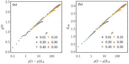
Figure 2: The scaling of (a) second Rényi entropy and (b) the von-Neumann entanglement entropy with the subsystem size for a Fermi sea of one dimensional spinless Fermions. Note the logarithmic scaling with the system size. The entanglement entropy vs subsystem size graph for Fermions at different densities $\rho$ collapse to a single graph when plotted as a function of $\rho(1-\rho)L_{A}$, where $L_{A}$ is the size of the subsystem

For a closed non-interacting system, $G^{R}(x,t;\alpha,0)=-i\Theta(t)\sum_{\mu}\phi_{\mu}(x)\phi^{\ast}_{\mu}(\alpha)\mathrm{e}^{-iE_{\mu}t}$, where $\mu$ denotes the eigenstates of the single-particle Hamiltonian with wavefunction $\phi_{\mu}$ and energy $E_{\mu}$. This leads to

$$\Gamma(x,x^{\prime},t)=\sum_{\alpha}G^{R}(x,t;\alpha,0)\left[G^{R}(x^{\prime},t;\alpha,0)\right]^{\ast}=\Theta(t)\delta_{x,x^{\prime}},$$ (42)

where we have used the orthonormality of wavefunctions $\sum_{\alpha}\phi_{\mu}(\alpha)\phi^{\ast}_{\nu}(\alpha)=\delta_{\mu,\nu}$ to get this answer. In this case, the entanglement entropies are given by

$$S^{(n)} = \frac{1}{1-n}\mathrm{Tr}\left[\ln\left[\hat{\Lambda}^{n}+(\hat{1}-\hat{\Lambda})^{n}\right]\right]$$

$$S_{vN} = -\mathrm{Tr}\left[\left[\hat{\Lambda}\ln\hat{\Lambda}+(1-\hat{\Lambda})\ln(1-\hat{\Lambda})\right]\right]$$ (43)

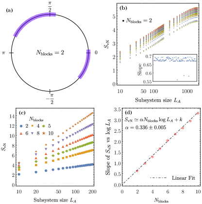
Figure 3: (a) A momentum Fock state of spinless Fermions in one dimension with $2$ contiguous blocks of occupied momenta. Note that under periodic boundary conditions, the Brillouin zone is mapped to a circle with circumference $2\pi/a$, where $a$ is the lattice spacing. (b) The scaling of von-Neumann entanglement entropy with subsystem size for Fock states with $2$ contiguous blocks. The slope of the logarithmic scaling is twice that for the Fermi sea ($y_{2}=2\times c/3$), where $c=1$ is the central charge for free Fermions. Inset: the value of the slope for each Fock state with $2$ contiguous blocks (plotted with configuration number). Note the lack of scatter in the slope, showing each $2$-block state has the same slope independent of the size or position of the blocks.(c) The scaling of entanglement entropy with subsystem size for Fock states with $p$ contiguous blocks with $p=2,4,5,6,8,10$. These states show logarithmic scaling with a coefficient which increases with $p$. (d) The coefficient of the logarithmic scaling plotted as a function of the number of blocks $p$, showing that the coefficient is simply $y_{p}=p\times c/3$. All the above data is for asystem with $L=4096$ sites and a density of $\rho=0.3$

While the above formulae are true for any closed system dynamics starting from Fock states, we will focus at $t=0$ where $\Lambda(x,x^{\prime},t=0)=\sum_{\alpha}n_{\alpha}^{0}\phi_{\alpha}(x)\phi^{\ast}_{\alpha}(x^{\prime})$. Here $n_{\alpha}^{0}$ is the occupation number of the mode $\alpha$ in the initial Fock state, and one gets the formula derived by Peschel et. al  Peschel (2003) using correlation matrix approach.

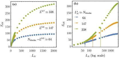
Figure 4: The scaling of entanglement entropy of momentum Fock states with subsystem size $L_{A}$ for states with $N_{b}=64$, $147$ and $338$ occupied blocks in a system with $4096$ lattice sites and a density of $\rho=0.3$. In (a) the subsystem size is on a linear scale, while in (b) the subsystem size is on a logarithmic scale. Note that at small values of $L_{A}$, the size dependence is linear (see (a)), which transitions to a logarithmic scaling for $L_{A}>N_{b}$, as seen in (b). The same states show critical or linear behaviour depending on the subsystem size.

We would like to point out one thing at the outset. If we consider a set of states $\{|n\rangle\}$, calculate the Rényi/von Neumann entanglement entropy for each one (with the same subsystem), and sample the entropy of the state $|n\rangle$ with probability $p_{n}$, this is not equal to the entanglement entropy of the density matrix $\hat{\rho}=\sum_{\{|n\rangle\}}p_{n}|n\rangle\langle n|$. For example, if $\hat{\rho}^{(n)}_{A}$ is the reduced density matrix obtained from $|n\rangle$, the first case yields $\mathrm{e}^{-S^{(2)}}=\sum_{n}p_{n}Tr\left[\hat{\rho}^{(n)}_{A}\right]^{2}$, while the second case yields $\mathrm{e}^{-S^{(2)}}=Tr\left[\sum_{n}p_{n}\hat{\rho}^{(n)}_{A}\right]^{2}$. This is in contrast to correlation functions, where these two procedures will yield the same result. For example, sampling all states with equal probability will not be equivalent to calculating entanglement entropy for an infinite temperature ensemble.

We consider momentum Fock states in a one dimensional lattice of spinless Fermions with periodic boundary conditions. In the thermodynamic limit, the momentum states are defined on a circle of circumference $2\pi/a$, where $a$ is the lattice spacing. In this case, $\hat{\Lambda}$ is a Toeplitz matrix generated by the momentum distribution (i.e. $\Lambda(x,x^{\prime},t=0)$ is the Fourier transform of the momentum distribution ). One can then use the Fisher Hartwig conjecture Basor and Morrison (1994); Alba et al. (2009), which relates the jump discontinuities in the generating function of a Toeplitz matrix to a power law scaling of its determinant with the dimension of the matrix. In this case, it relates the jump discontinuities to a logarithmic scaling of the entanglement entropies with the subsystem size $L_{A}$ (which is the dimension of the matrix $\Lambda$). For example, it is well known that the Fermi sea , which is a contiguous line of momentum occupancies with two jump discontinuities at the two ends, leads to a logarithmic dependence of the entanglement entropy with the subsystem size, with a coefficient related to the central charge of the corresponding conformal field theory, $c$: $S^{(2)}=\frac{c}{4}\ln~{}L_{A}$ and $S_{vN}=\frac{c}{3}\ln~{}L_{A}$ Calabrese and Cardy (2004), where $c=1$ for two species (left and right moving) of fermions in the system.

We consider a system of $L=4096$ lattice sites with different number of particles $N$, leading to different densities $\rho=N/L$. In Fig  2(a) and (b), we plot the Rényi and von Neumann entanglement entropy of the one dimensional Fermi sea as a function of the subsystem size $L_{A}$ to show the logarithmic scaling. We note that the curves for different densities collapse when plotted as a function of $\rho(1-\rho)L_{A}$. For closed fermionic systems, one can either describe the system in terms of particles created on top of a vacuum state with zero particles, or in terms of holes created on top of a state with all single particle modes filled. Thus, there is an invariance under $\rho\rightarrow 1-\rho$, which is reflected in the collapse of the curves when plotted as a function of $\rho(1-\rho)L_{A}$.

We now consider a Fock state made of two contiguous blocks of occupied momentum states. To see what this means, we show a Fock state with $N_{b}=2$ contiguous blocks of occupation in Fig 3(a). The entanglement entropy of this state is $S_{vN}=2\times\frac{c}{3}\ln~{}L_{A}$, as there are now four jump discontinuities in the momentum distribution. This answer does not depend on the size of the occupied blocks, their locations or the separation between them, and only cares about the number of jump discontinuities, just as Fisher Hartwig conjecture would predict. In Fig. 3(b), we plot the entanglement entropy of several of these “2-block” states with the subsystem size. The logarithmic scaling is obtained with a coefficient which is twice the coefficient for the Fermi sea. The value of this coefficient (slope of the curve), obtained for different “2-block” states, is shown in the inset of Fig. 3(b) as a function of the configuration number for about $100$ such states. The absence of scatter shows that each state follows the logarithmic scaling with the same co-efficient. We note that the intercept of the curve is non-universal and varies widely from one Fock state to another.

This argument can now be extended to the case of Fock states with $p$ contiguous blocks of momentum occupancy, which will have $S_{vN}=p\times\frac{c}{3}\ln~{}L_{A}$. In Fig. 3(c), we plot the entanglement entropy of Fock states with $p$ contiguous blocks of occupancy for $p=2,4,..10$ as a function of $L_{A}$ and show that the logarithmic scaling with the subsystem size is recovered. In Fig. 3(d), we plot the slope of the curve with $p$ to see that the coefficient matches our expectations. For each value of $p$ we have averaged over $20$ random configurations of the blocks and the variation of the slope from configuration to configuration is negligible. This suggests a classification of the “critical states” in terms of number of contiguous occupied blocks in the momentum space, $N_{b}$. We note that this classification is similar to the one proposed by Ref. Alba et al., 2009 and is different from that of Jafarizadeh et. al Jafarizadeh and Rajabpour (2019), since our states do not have any periodic arrangements in momentum space.

However, when we extend the above construction to states with larger number of contiguous blocks, a more comprehensive picture emerges. If we consider the entanglement entropy of Fock states with a particular value of $N_{b}$ as a function of the subsystem size $L_{A}$ (for $L_{A}/L\ll 1$), then:(i) $S_{vN}(N_{b})\sim N_{b}\times\frac{c}{3}\ln~{}L_{A}$ for $L_{A}\gg N_{b}$ and (ii) $S_{vN}(N_{b})\sim L_{A}$ for $L_{A}\ll N_{b}$, and the dependence on the subsystem size has a smooth crossover from linear to logarithmic around $N_{b}\sim L_{A}$. This is shown in Fig 4(a) and (b), where the entanglement entropy of states with $N_{b}=64$, $147$ and $338$ are plotted as a function of $L_{A}$ on linear and logarithmic scales respectively. We have used a system size of $L=4096$ and a density of $\rho=0.3$ for these plots. We clearly see that the dependence goes from linear to logarithmic and the change happens at $L_{A}\sim N_{b}$. We note that the Fisher Hartwig conjecture works for a finite number of singularities (compared to size of the matrix), and hence it is not surprising that it breaks down when number of discontinuities in the generating function is larger than the system size.

The key insight that we get from the above exercise is that there are no “critical” or “non-critical” states. The same quantum state can show either critical (logarithmic dependence on $L_{A}$) or non critical (linear dependence on $L_{A}$) behaviour of entanglement entropy depending on the size of the subsystem. For a given subsystem size, however, we can divide states into those which show logarithmic and linear dependence of entanglement entropy. Every Fock state can be written as the ground state of some non-interacting Hamiltonian and Alba et. al Alba et al. (2009) had showed that if this Hamiltonian is long ranged, then the entanglement entropy scales linearly with subsystem size, while a short range Hamiltonian results in a logarithmic scaling. In that language, the above results show that if the subsystem size is longer than the range of this Hamiltonian, the state will show critical behaviour in the scaling of the entanglement entropy. Note that this also points out the difficulty of obtaining these estimates numerically, since there is a strong subsystem size dependence of the results.

We will now estimate the number of these “critical” states (for a given $L_{A}$, and states with $N_{b}<L_{A}$) in a system with $N$ particles on $L$ sites. The first thing to note is that in general $1\leq N_{b}\leq\min(N,L-N)$. Since each occupied block has to be followed by an empty block, the number of blocks is bounded by the number of particles/holes in the system. Let us first consider the number of possible states with $N_{b}$ blocks. This problem is equivalent to the number of ways of choosing $N_{b}$ out of $N$ positions amongst the occupied momenta to place the boundaries of the blocks, multiplied by the number of ways of choosing $N_{b}$ out of $L-N$ positions amongst the unoccupied momenta to assign the gaps between the occupied blocks. So the total number of states with $N_{b}=Lx$ blocks is

$$\Omega(N_{b}) = \frac{N!}{(N-N_{b})!N_{b}!}\frac{L-N!}{(L-N-N_{b})!N_{b}!}$$

$$\sim \frac{\mathrm{e}^{-L[2x\ln x+(\rho-x)\ln(\rho-x)+(1-\rho-x)\ln(1-\rho-x)]}}{\mathrm{e}^{-L[\rho\ln\rho+(1-\rho)\ln(1-\rho)]}}$$

where we have used the thermodynamic limit with $N=L\rho$. in the last line. The number of critical states is obtained by summing over this expression for $0<x<\alpha$, where the subsystem size $L_{A}=L\alpha$. Now in general one requires $\alpha\ll 1$ for the critical logarithmic scaling to hold (this is the limit in which conformal invariance is preserved). So we expect an exponentially large number of “critical” states, although they will form a vanishing fraction of the total number of states, unless $L_{A}/L$ is a substantial fraction, in which case one needs to worry about corrections due to finite $L_{A}/L$.

VII Entanglement Dynamics in Open Quantum Systems

In this section, we will finally use our formalism to compute the dynamics of entanglement entropy in an open quantum system of Fermions. We will see how the entanglement entropy bears the signatures of different classical and quantum processes during the evolution of the system.

We consider a one dimensional lattice of spinless Fermions with nearest neighbour hopping and free boundary conditions

$$H_{s}=-g\sum_{i=1}^{L-1}c^{\dagger}_{i+1}c_{i}+h.c.$$ (45)

where $i$ indicate the lattice site and $g$ is the hopping amplitude which sets the bandwidth of the system. At $t=0$, the system is in a Fock state described by occupation number of each lattice site. The particular initial condition we choose here is the following: Sites $1$ to $L/2$ are filled with $1$ particle, while sites $L/2+1$ to $L$ are empty. This is shown in Fig. 5(b). We note that the spinless Fermi gas in one dimension can be mapped to a spin system. In that language, our initial condition corresponds to a domain wall at the center of the system.

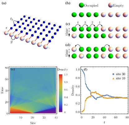
Figure 5: (a) A schematic diagram of a one dimensional Fermionic chain with nearest neighbour hopping $g$, with each site coupled to a Fermionic bath represented by one dimensional chains with hopping $t_{B}$. The system bath coupling is $\epsilon$. (b) The initial real space Fock state with the left half of the system filled with $1$ particle per site and the right half kept empty. The system has $L=40$ sites. There is a domain wall at the center of the system. (c-d) The different physical processes during the non-equilibrium dynamics of this open quantum system: (c) Coherent motion of a domain wall wavefront across the system and (d) Breaking of a single domain into multiple domains and vice-versa. In addition every site can exchange energy and particles with the local bath (e) A color plot of the evolution of the density profile of the system after it is coupled to an external bath at $t=0$. The propagation of the wavefront of domain walls lead to the characteristic diamond shapes in the color plot. (f) The density profile of two sites located symmetrically from the center on the left and right. The initial in(de)crease is due to exchange of particles with the bath, whereas the sharp jumps correspond to the passing of a domain wavefront. The oscillations correspond to breaking up of a single domain into two and vice-versa. The coherent motion gets damped and settles into a homogeneous value for the density at long times. The graphs correspond to parameters $g=1.0$, $t_{B}=2.0$, $\epsilon=0.2$. The bath temperature is $T=1.0$ and chemical potential $\mu=-1.11$, so that the equilibrium density of the system is $\rho_{eq}=0.32$ in this case.

At $t=0$ we also turn on the coupling of this system to an external bath of Fermions with which it can exchange energy and particles. Each site of the system couples to a bath, which is modelled as another linear chain of free Fermions with a nearest neighbour hopping scale $t_{B}$. The system bath coupling is linear and is controlled by a parameter $\epsilon$. A schematic of the system , the bath and the system bath coupling is shown in Fig 5(a). The details of this model is the same as that used in Ref Chakraborty and Sensarma, 2018b, which was used to study the dynamics of correlation functions in the system. The effect of the bath on our system is characterized by the spectral function of the bath $J(\omega)$, its temperature $T$ and its chemical potential $\mu$. In the long time limit, we expect our system to thermalize with this bath with a density determined by $T$, $\mu$ and $g$. For our specific model of the bath, the spectral density is given by $J(\omega)=\Theta(4t_{B}^{2}-\omega^{2})\frac{2}{t_{B}}\sqrt{1-\omega^{2}/4t_{B}^{2}}$, with a band width of $4t_{B}$. The band edge singularities of this spectral function leads to non-Markovian dynamics in this system  Chakraborty and Sensarma (2018b). Throughout this section, we will consider a lattice of $L=40$ sites. Our system will be characterized by a hopping strength $g=1.0$, while the bath is characterized by a hopping $t_{B}=2.0$ (making sure bath bandwidth is larger than system bandwidth, so that it acts as a heat bath for all modes in the system), a temperature $T=1.0$ ( we take $k_{B}=1$) and a chemical potential $\mu=-1.1$, which corresponds to a bath particle density of $0.4$. If the system thermalizes with the bath, it should have a density of $0.32$, as compared to an initial density of $n=0.5$. The system bath coupling is set to $\epsilon=0.2$.

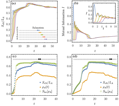
Figure 6: (a) The time evolution of entanglement entropy of $2$-site subsystems located at various distances $\delta$ from the center of the system. The subsystems are shown as colored dots, and the entropy of the corresponding subsystem is plotted with same color. After an initial common rise, the curves show a sudden rise at different times corresponding to the time the wave front passes through this subsystem. (b) The mutual information between the two $1$-site subsystems that make up the $2$ site subsystems shown in (a). The sharp rise and the oscillations are prominent here. Inset: a close up of the small time dynamics of the mutual information showing that it rises at different times for subsystems at different distances from the center. (c) and (d) The time evolution of average density $\rho_{A}$ (yellow) and entanglement entropy density $S_{vN}/L_{A}$ (blue) of a $2$-site subsystem starting at the (c) $24^{th}$ and (d)$35^{th}$ site. The green curve is $S_{loc}$, which is the entropy of an effective one site subsystem with the average density. The graphs correspond to a system hopping $g=1.0$, a bath hopping $t_{B}=2.0$, a system bath coupling $\epsilon=0.2$. The bath temperature $T=1.0$ and chemical potential $\mu=-1.11$, so that the equilibrium density of the system is $\rho_{eq}=0.32$ in this case.

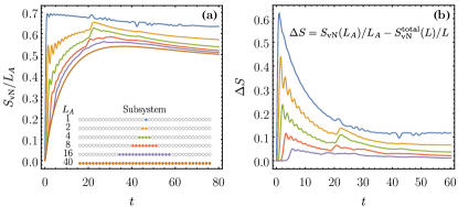
Figure 7: (a) Evolution of entanglement entropy (per site) $S_{vN}/L_{A}$ of subsystems, of different sizes, $L_{A}=1$, $2$, $4$, $8$, $16$, and $40$ (whole system), located in the central part of the system. Note the sharp jump occuring at different initial times for different subsystems coupled with oscillations. These features are absent when $L_{A}=40$, i.e. the whole system is considered. (b) The time evolution of $\Delta S$, the excess entropy per site of the subsystems, as measured from the entropy per site of the whole system. This measures the additional entropy obtained due to tracing of degrees of freedom. The graphs correspond to a system hopping $g=1.0$, a bath hopping $t_{B}=2.0$, a system bath coupling $\epsilon=0.2$. The bath temperature $T=1.0$ and chemical potential $\mu=-1.11$, so that the equilibrium density of the system is $\rho_{eq}=0.32$ in this case.

As this open quantum system evolves, we track the dynamics of entanglement entropy in the system with the formalism we have developed. There are three distinct processes that happen and leave their imprint on both the correlation functions and entanglement measures in the system. The first is an exchange of particles between the system and the bath, which changes the imposed density pattern in the system. This is a local and incoherent process depicted in figure 5(a). The second process corresponds to creation of two domain walls at the center which spread outwards like a wavefront, leading to a domain of particles going right and a domain of holes going left. This is schematically depicted in 5(c). These wavefronts are then reflected back from the boundaries towards the center. This is equivalent to sloshing of particle and hole domains in the system and is a coherent quantum process. The waves are damped due to the incoherent exchange with the bath and eventually die off. The third process that happens is the creation and annihilation of additional domain walls due to hopping of the particles, resulting in local Rabi oscillations in the system. This mechanism, depicted in Fig 5(d) is also a coherent quantum process.

Let us first focus on the evolution of the density profile in this system. In Fig 5(e), we plot the particle density as a function of space and time in a color plot. The wavefront dynamics is clearly visible as a sharp jump in the density profile, which propagates outward from the center with a uniform velocity. On the right hand section of the lattice, which starts with no particles, the jump leads to an increase in the density, while it leads to a decrease in density on the left half which starts with a local density of $1$. This is equivalent to a particle and a hole domain moving outward. The reflection of the waves from the boundary leads to the characteristic diamond shape in the figure. The creation and annihilation of domain walls create subsidiary wavefronts, leading to the additional ripples seen in the pattern. Finally the settling down of the wave is due to damping coming from interaction with the bath. We note that the wavefront velocity $v\sim 1.9~{}ga$, whereas the subsequent ripples give a timescale $\tau_{r}\sim g^{-1}$, as expected from the hopping scale in the problem. This is clearly seen in Fig. 5(f), where we plot the time evolution of density of a single site on the left and right half of the system. The sharp jumps correspond to the wavefront passing through the site, while the oscillations, which occur after the initial wavefront has passed, have a frequency $\sim g$. The damping of the coherent motion occurs on the dissipation time scale provided by the bath, $\tau_{B}\sim 2t_{B}/\epsilon^{2}=20$, as seen from Fig. 5 (e) and (f).

We now shift our focus to the dynamics of entanglement measures in this system. In Fig. 6(a), we plot the von-Neumann entanglement entropy per site of several 2 site subsystems of our open quantum system as a function of time. These two sites ($[i,i+1]$) are next to each other, but their location is varied from the center outward towards the right. Defining $\delta=i-L/2$, i.e. the distance from the center, the curves correspond to $\delta=0$ (blue), $\delta=2$ (orange), $\delta=4$ (green), $\delta=6$ (red), and $\delta=8$ (purple), as shown in Fig. 6(a). The entropy starts at zero, as expected for a product state, and there is an initial rise which is independent of the location of the subsystem. This is dominated by the exchange of particles with the bath and consequent hopping of these particles between the two sites. Then, there is a sharp rise in the entanglement entropy of the subsystem when the wavefront of the domain sloshing passes through the subsystem. This sharp rise happens at a later time as we move the subsystem outwards from the center, and the time of the jump coincides with the time when the average density in the subsystem also shows a jump, as shown in Fig. 6(c) & (d). We can thus correlate this feature with the passing of the wavefront. The entanglement entropy then rises slowly with a shoulder like feature, which has oscillations superimposed on it. During this time the system is undergoing local Rabi oscillations between nearest neighbours leading to creation and annihilation of additional domains in the system. The incoherent exchange with the bath is also active during this time. One can again see a sharp jump around $t=20$, when the reflected wave passes through the subsystem. Note that this jump occurs first for subsystems farther from the center, since the reflected wave reaches this point earlier. Beyond this point, the entanglement entropy settles into a long time decay to its final equilibrium value. During this time, the entanglement entropy is independent of the location of the subsystem, since the local incoherent exchange with the bath is dominating the dynamics during this period.

We have seen that there is a clear correlation between features in the dynamics of density and entanglement entropy of the system. An obvious question is whether one can explain the dynamics of the entanglement entropy solely in terms of the density dynamics. To explore this question, note that for a spinless system, fixing the density of a $1$ site subsystem fixes its density matrix, and hence its entanglement entropy. If the density is $\rho$, this local entanglement entropy $S_{\text{loc}}=-[\rho\ln\rho+(1-\rho)\ln(1-\rho)]$. Thus, we can compare the entanglement entropy of the two site subsystem with that of an effective one site subsystem with the same average density. The difference will be related to entanglement between the two sites making up the subsystem. In Fig 6(c), we plot the entanglement entropy and average density of a $2$-site subsystem starting at the $24^{th}$ site (this is to the right of the center) as a function of time. In the same figure, we also plot the entropy of an effective $1$-site subystem with average occupation $\rho(t)$, i.e.

$$S_{\text{loc}}(t)=-[\rho(t)\ln\rho(t)+(1-\rho(t))\ln(1-\rho(t))].$$ (46)

We see that these two curves fall on top of each other till the first coherent wave hits the subsystem, and then they differ from each other, while following the same general trends. Similar trends can be seen for another two site subsystem starting on the $35^{th}$ site in Fig 6(d). In this case, the coherent wave passes later and hence the entanglement entropy follows $S_{\text{loc}}$ for a longer time. This reconfirms the idea that the initial dynamics is incoherent till the domain wall wavefront hits the subsystem.

A better way to distinguish the entanglement between the degrees of freedom in the subsystem is to calculate the mutual information. For the two site subsystem composed of site $i$ and site $i+1$, the mutual information between the sites, $I$ is given by

$$I(i,i+1)=S_{\text{vN}}(i,i+1)-S_{\text{vN}}(i)-S_{\text{vN}}(i+1),$$ (47)

where $S_{\text{vN}}(i,i+1)$ is the entanglement entropy of the two state system, $S_{\text{vN}}(i)$ and $S_{\text{vN}}(i+1)$ are the entanglement of the corresponding single site systems. This quantity would be zero if the two sites are not entangled. The mutual information between the two consecutive sites at different locations are plotted as a function of time in Fig 6(b). We have plotted the mutual information for the same set of subsystems for which entanglement entropy was plotted in Fig 6(a) with the same color coding. In this case, we find large jumps with oscillations superimposed on an increasing background. The background is independent of the location of the subsystem. This comes from the change in particle density due to exchange with the bath, and these particles getting entangled by hopping. The initial jumps coincide with the passing of the coherent wavefront and occurs later for subsystems which are located farther from the center. This is shown in the inset of Fig 6(b) for small times. The mutual information decays with some oscillations (created by breaking up of the domain walls) and finally settles to the background once this wave is damped around $t=20$. The mutual information thus cleanly picks up the quantum coherence on top of the increasing background due to incoherent exchange with the bath and subsequent coupling of the sites due to hopping.

We now focus on how the evolution of the entanglement entropy is affected by the size of the subsystem. For this we consider subsystems of increasing size centered around the middle of the system. The time evolution of the entanglement entropy density (i.e. the entanglement entropy divided by the subsystem size) of different sized subsystems is plotted in Fig 7(a). The different sizes plotted are $L_{A}=1$ (blue), $L_{A}=2$ (orange), $L_{A}=4$ (green), $L_{A}=8$ (red), $L_{A}=16$ (purple), and $L_{A}=40$ (brown), which corresponds to the whole system. While the entanglement entropy of the subsystems show the sudden jump and oscillations evident in the two site systems, the amplitude of these oscillations go down as we look at larger and larger subsystems. In fact the evolution of entropy for the full system is smooth and devoid of these features. The finite subsystems follow this curve upto a point and then deviate to manifest the effects of quantum processes in the system.

When we calculate the entanglement entropy of a subsystem in a pure quantum state, it has a simple interpretation: the loss of information about the quantum degrees of freedom shows up as entropy of the reduced density matrix. However in an open quantum system, the whole system evolves from a pure state to a density matrix and has an entropy of its own (the $L=40$ curve shows evolution of this entropy). To take this into account, we define the excess entropy density of a subsystem,

$$\Delta S=\frac{S_{\text{vN}}(L_{A})}{L_{A}}-\frac{S_{\text{vN}}(L)}{L}.$$ (48)

This is the additional randomness introduced into the subsystem due to tracing of the complementary degrees of freedom. In Fig 7(b), we plot the time evolution of $\Delta S$ for different subsystem sizes (with same color coding as Fig 7(a)). We see that this excess entropy shows a steep jump followed by a decay with oscillations superposed on it. The characteristic jumps due to passing of the wavefront is clearly evident in this plot. We also note that in the long time limit, it is clear that the smaller subsystems have more excess entropy density. This is expected since we are tracing over larger number of degrees of freedom in this case, leading to more information loss.

VIII Conclusions

In this paper, we have formulated a new way of calculating entanglement entropy of Fermionic systems through the construction of a Wigner functio,n which is a Grassmann valued function of Grassmann variables. The Wigner function is then identified with the Keldysh partition function of the system with a set of sources, which are proportional to the arguments of the Wigner function.

We have extended this formalism to non-equilibrium dynamics starting from arbitrary initial conditions. For a non-interacting fermionic open quantum system, starting from an initial Fock state, we have derived exact formulae for the entanglement entropy of a subsystem. This is the key new universal result in this paper, which has a wide scope of application in different situations.

We have used our formalism to look at entanglement entropy of momentum Fock states of one-dimensional Fermions. We find that the states can be classified by the number of contiguous blocks of momentum occupancy in them. This is also related to the number of zeroes in the dispersion of the effective Hamiltonian, for which this Fock state is a ground state. If the number of momentum occupancy blocks is smaller than the size of the subsystem, the entanglement entropy of the subsystem scales logarithmically with the subsystem size, and the state looks “critical”; i.e. shares the property of many body systems at phase transitions. On the other hand when the number of blocks is larger than the subsystem size, the entanglement entropy scales linearly with the subsystem size, which is a typical property of thermal systems. So, the same state can either look “critical” or “thermal” depending on the range of subsystem size one is looking at. We use this idea to analytically estimate the number of “critical” states for a given subsystem size.

Finally, we use our formalism to study the evolution of entanglement entropy of subsystems of a one dimensional open quantum system, which is initialized to a state with a domain wall at the center of the lattice. We understand the dynamics in terms of the coherent motion of the domain walls together with incoherent exchange of particles with the bath.

We would like to note that the formulae that we have derived in this paper are applicable to a large class of systems under different situations. They will especially help in understanding behaviour of entanglement entropy in higher dimensional systems, where there are very few answers known, but we leave this question for a future work,

Appendix A Wigner Characteristic and Diagrammatic Expansion of Rényi Entropy

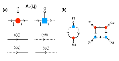
Figure 8: (a) Vertices and propagators used in evaluating the second Rényi entropy. Note that the solid lines begin and end at circular vertices, while the dotted lines begin and end at the square vertices. The third line from the vertices (ending in a small circle) is used to denote the mode or $\alpha$ index of the vertex. The lines coming from the vertices are joined to form propagators. The four kinds of propagators are indicated in the figure. (b) A disconnected diagram for the evaluation of $\mathrm{e}^{-S^{(2)}}$. Note that the indices of the circular vertices are constrained to be $\alpha_{1}\neq\alpha_{2}\neq\alpha_{3}$. Similarly, the indices of the square vertices must satisfy $\gamma_{1}\neq\gamma_{2}\neq\gamma_{3}$. These constrained summations make evaluation of these diagrams difficult.

In this section, we will provide an alternative derivation of the formulae derived above, which will also indicate a way forward for the case where the number of particles is smaller than the subsystem size. In this case, we will first obtain the Wigner characteristic function by taking the derivatives with respect to initial sources in Eq. 24 to write

$$\chi_{D}(\bm{\zeta},\bm{\bar{\zeta}},t)=\mathrm{e}^{-\frac{1}{2}\bm{\bar{\zeta}}\hat{\Gamma}(t)\bm{\zeta}}\prod_{\alpha}[1+n_{\alpha}\bm{\bar{\zeta}}\hat{\Lambda}^{\alpha}(t)\bm{\zeta}]$$ (49)

where $\bm{\bar{\zeta}}=(\bar{\zeta}_{x_{1}},\bar{\zeta}_{x_{2}}...\bar{\zeta}_{x_{V_{A}}})$, and $\hat{\Gamma}$ and $\hat{\Lambda}$ are matrices in $x$,$x^{\prime}$ space. The second Rényi entropy is then given by

$$\mathrm{e}^{-S^{(2)}}=\int{\cal D}[\bm{\zeta},\bm{\bar{\zeta}}]{\cal D}[\eta,\bar{\eta}]\mathrm{e}^{-\frac{1}{2}\left(\bar{\bm{\zeta}},\bar{\bm{\eta}}\right)\left(\begin{array}[]{cc}\hat{\Gamma}(t)&-\hat{1}\\ \hat{1}&\hat{\Gamma}(t)\end{array}\right)\left(\begin{array}[]{c}\bm{\zeta}\\ \bm{\eta}\end{array}\right)}\prod_{\alpha}[1+n_{\alpha}\bm{\bar{\zeta}}\hat{\Lambda}^{\alpha}(t)\bm{\zeta}]\prod_{\gamma}[1+n_{\gamma}\bm{\bar{\eta}}\hat{\Lambda}^{\gamma}(t)\bm{\eta}]$$ (50)

where $n_{\alpha}$ is the occupation number of the mode $\alpha$ in the initial state. The appearance of integrals of a gaussian function multiplied by polynomials in Eq. 50 suggest the use of Wick’s theorem and resultant diagrammatic representations to evaluate $\mathrm{e}^{-S^{(2)}}$. The key elements of this expansion are shown in Fig.  8. The vertices $n_{\alpha}\hat{\Lambda}^{\alpha}$ coupling to the $\bm{\bar{\zeta}},\bm{\zeta}$ variables is represented by a circle with three legs sticking out; the top leg ending in a small circle indicates the label $\alpha$, which we will refer to as “index” of the vertex. The horizontal outgoing leg indicates the coupling to $\bm{\bar{\zeta}}$ and the horizontal incoming leg indicates the coupling to$\bm{\zeta}$. Similar construction is done with square vertices for $n_{\gamma}\hat{\Lambda}^{\gamma}$ s coupling to $\bm{\bar{\eta}},\bm{\eta}$ variables. Note that the $\bm{\bar{\zeta}},\bm{\zeta}$ variables are denoted by thick lines, while $\bm{\bar{\eta}},\bm{\eta}$ variables are denoted by dashed lines. While the square and circular vertices represent the same matrix, it is useful to keep them as separate vertices for various book keeping purposes. These are shown in Fig.  8(a). Fig. 8 (a) also shows the propagators: the expectation $\langle\zeta\bar{\zeta}\rangle=2\left[\hat{1}+\hat{\Gamma}^{2}\right]^{-1}\hat{\Gamma}$ is denoted by a thick straight line, $\langle\eta\bar{\eta}\rangle=2\left[\hat{1}+\hat{\Gamma}^{2}\right]^{-1}\hat{\Gamma}$ by a dashed straight line, $\langle\eta\bar{\zeta}\rangle=-2\left[\hat{1}+\hat{\Gamma}^{2}\right]^{-1}$ is denoted by a dashed-thick line and $\langle\bar{\eta}\zeta\rangle=2\left[\hat{1}+\hat{\Gamma}^{2}\right]^{-1}$ is denoted by a thick-dashed line. The diagrams for $\mathrm{e}^{-S^{(2)}}$ then correspond to motifs where no lines are hanging out (much like diagrams for partition functions in standard field theories). They are composed of rings with square and circular vertices sitting on them. Note that a diagram for $\mathrm{e}^{-S^{(2)}}$ can consist of several such disconnected rings. One such diagram is shown in Fig. Fig.  8 (b).

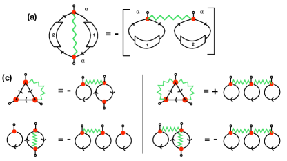
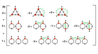
Figure 9: (a) Vertices and propagators used in evaluating the second Rényi entropy. Note that the solid lines begin and end at circular vertices, while the dotted lines begin and end at the square vertices. The third line from the vertices (ending in a small circle) is used to denote the mode or $\alpha$ index of the vertex. The lines coming from the vertices are joined to form propagators. The four kinds of propagators are indicated in the figure. (b) A disconnected diagram for the evaluation of $\mathrm{e}^{-S^{(2)}}$. Note that the indices of the circular vertices are constrained to be $\alpha_{1}\neq\alpha_{2}\neq\alpha_{3}$. Similarly, the indices of the square vertices must satisfy $\gamma_{1}\neq\gamma_{2}\neq\gamma_{3}$. These constrained summations make evaluation of these diagrams difficult.

The rules for evaluating a particular diagram can be given by: (i) For each vertex put the corresponding $n_{\alpha}\hat{\Lambda}_{\alpha}$ matrix (in $x$,$x^{\prime}$ space). (ii) For each propagator multiply by the corresponding matrix; keep the order of multiplication intact since $\hat{\Gamma}$ and $\hat{\Lambda}_{\alpha}$ do not commute when there is a Keldysh self-energy due to coupling to an external bath. (iii) For each ring, take the trace of this product in the $x$, $x^{\prime}$ space and multiply. (v) Multiply by $(-1)^{F}$, where $F$ is the number of Fermion loops (in this case, number of disconnected rings). (iv) For each diagram, multiply by the symmetry factor, which is the number of different connections which produce the same diagram. (vi) Sum over all possible $\alpha$ s and $\gamma$ s of the $\Lambda$ matrices, making sure that all $\alpha$ values are distinct and all $\gamma$ values are distinct. (vii) This last constraint comes from expanding the product

$$\prod_{\alpha}\left[1+n_{\alpha}\bar{\zeta}_{x}\hat{\Lambda}^{\alpha}(xx^{\prime})\zeta_{x^{\prime}}\right]=1+\sum_{\alpha}n_{\alpha}\bar{\zeta}_{x}\hat{\Lambda}^{\alpha}(xx^{\prime})\zeta_{x^{\prime}}+\frac{1}{2!}\sum_{\alpha\neq\beta}n_{\alpha}\bar{\zeta}_{x_{1}}\hat{\Lambda}^{\alpha}(x_{1}x^{\prime}_{1})\zeta_{x^{\prime}_{1}}n_{\beta}\bar{\zeta}_{x_{2}}\hat{\Lambda}^{\beta}(x_{2}x^{\prime}_{2})\zeta_{x^{\prime}_{2}}+\cdots.$$ (51)

The constrained sum leads to great difficulties in evaluating the diagrams; since one cannot treat the $\alpha$ and $\gamma$ indices as internal indices to be summed over independently, one has to evaluate the diagrams resulting from all the permutations of these indices separately, leading to exponential growth in number of diagrams.

We note that a-priori there is no small parameter in this expansion and hence it does not make sense to evaluate a few diagrams.

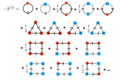
Figure 10: The series of connected diagrams for calculation of $S^{(2)}$

However, for the case of Fermions, one can get rid of the constrained summations by the following argument: The constrained sums over distinct pairs can be written in terms of unconstrained sums and identification of variables, e.g. $\sum_{(a,b)}f(a,b)=\frac{1}{2!}\left[\sum_{ab}f(a,b)-\sum_{a}f(a,a)\right]$ and so on, where $(a,b)$ denote distinct pairs. Thus the constrained summation can be overcome at the expense of having additional diagrams, where some of the circular (or square) vertices are identified. We denote such an identification by putting a wavy line joining the vertices. Fig.  9 (a) shows all diagrams (with associated symmetry factors) with three circular vertices in the expansion of $\mathrm{e}^{-S^{(2)}}$, written in terms of identified vertices. Note that diagrams can have more than two vertices identified.

The matrix $n_{\alpha}\hat{\Lambda}_{\alpha}$ has a factorizable form, i.e. $\hat{\Lambda}^{\alpha}(x,x^{\prime})\sim g_{\alpha}(x)g^{\ast}_{\alpha}(x^{\prime})$ and $n_{\alpha}^{2}=n_{\alpha}$. Using this, one can then easily show that $\mathrm{Tr}\left[\hat{\Lambda}^{\alpha}\hat{A}\hat{\Lambda}^{\alpha}\hat{B}\right]=\left(\mathrm{Tr}\left[\hat{A}\hat{\Lambda}^{\alpha}\right]\right)\left(\mathrm{Tr}\left[\hat{B}\hat{\Lambda}^{\alpha}\right]\right)$ for any matrices $\hat{A}$ and $\hat{B}$. In terms of diagrams, this implies that a ring, where two indices are identified, is equal to negative of a “disconnected” diagram with two rings each involving one of the indentified vertices. This is shown in Fig.  9 (b). The negative sign comes because the equivalent “disconnected” diagram has an extra fermion loop, while the Trace factorization does not give any minus sign. With this, one can show that diagrams with any non-zero number of identifications cancel each other. For example, the equivalences between the diagrams in Fig.  9 (a) are shown in Fig.  9 (c). It is easy to see from a simple counting that the diagrams in Fig.  9 (a) with the wavy lines sum to zero. This cancellation works out for each set of diagrams which has $n$ circular vertices and $m$ square vertices (these include disconnected diagrams of a particular “order”). Note that the Fermion minus sign is crucial for this cancellation, and this would not occur for a similar construction with Bosons.

The net result of the cancellation described above is that we can simply replace the “distinct pair summations” over the indices by unconstrained summations. Since the propagators do not depend on the index, this allows us to replace every vertex by $\hat{\Lambda}=\sum_{\alpha}n_{\alpha}\hat{\Lambda}^{\alpha}$, and hence we can now drop the line on the vertices ending in a small circle, which was used to indicate the index. Going back to the integral which gave rise to this diagrammatics, we can now write it as

$$\mathrm{e}^{-S^{(2)}}=\int{\cal D}[\bm{\zeta},\bm{\bar{\zeta}}]{\cal D}[\bm{\eta},\bm{\bar{\eta}}]~{}\mathrm{e}^{-\dfrac{1}{2}\begin{matrix}\begin{pmatrix}\bm{\bar{\zeta}}&\bm{\bar{\eta}}\end{pmatrix}\\ \hskip 2.0pt\end{matrix}\left(\begin{array}[]{cc}\hat{\Gamma}(t)&-\hat{1}\\ \hat{1}&\hat{\Gamma}(t)\end{array}\right)\left(\begin{array}[]{c}\bm{\zeta}\\ \bm{\eta}\end{array}\right)}\sum_{l=0}^{N}\frac{\left[\bm{\bar{\zeta}}\hat{\Lambda}(t)\bm{\zeta}\right]^{l}}{l!}\sum_{m=0}^{N}\frac{\left[\bm{\bar{\eta}}\hat{\Lambda}(t)\bm{\eta}\right]^{m}}{m!}$$ (52)

We note that the number of Grassmann variables $\zeta_{x}$ (and $\eta_{x}$) is $L_{A}$. Hence for $l>L_{A}$, $\left[\bm{\bar{\zeta}}\hat{\Lambda}(t)\bm{\zeta}\right]^{l}$ inevitably repeats one or more $\zeta_{x}$ s in the string, and the string is then zero by definition. For $N\geq L_{A}$, this allows us to extend the summation over $l$ or $m$ in Eq. 52 to $\infty$ and we get a factor of $\mathrm{e}^{\bm{\bar{\zeta}}\hat{\Lambda}(t)\bm{\zeta}+\bm{\bar{\eta}}\hat{\Lambda}(t)\bm{\eta}}$ from the polynomials. Combining with the Gaussian part, this gives

$$\mathrm{e}^{-S^{(2)}}=\int{\cal D}[\bm{\zeta},\bm{\bar{\zeta}}]{\cal D}[\bm{\eta},\bm{\bar{\eta}}]~{}\mathrm{e}^{-\dfrac{1}{2}\begin{matrix}\begin{pmatrix}\bm{\bar{\zeta}}&\bm{\bar{\eta}}\end{pmatrix}\\ \hskip 2.0pt\end{matrix}\left(\begin{array}[]{cc}\hat{\Gamma}(t)-2\hat{\Lambda}(t)&-\hat{1}\\ \hat{1}&\hat{\Gamma}(t)-2\hat{\Lambda}(t)\end{array}\right)\left(\begin{array}[]{c}\bm{\zeta}\\ \bm{\eta}\end{array}\right)}$$ (53)

which leads to the formula Eq. 39.

Further, if we assume that the number of particles $N$ goes to infinity, the series does not terminate after a finite number of terms. Then we can use the linked cluster theorem to show that the expansion for $S^{(2)}$ will only have connected diagrams, i.e. single rings with different arrangement of square and circular vertices. The first few terms in this series (upto $4^{th}$ order in $\hat{\Lambda}$ has been shown in Fig. 10. The diagram evaluation rules are same as before with two additional rules: (a) vertices are represented by $\hat{\Lambda}$ and (b) an additional factor of $1/{m!n!}$ multiplies diagrams with $m$ circular and $n$ square vertices.

Appendix B Derivation of Formulae for $S^{(n)}$ and $S_{vN}$

In this Appendix, we show the derivation of the formulae for $S^{(n)}$ which has been quoted in the main text. The proof follows the essence of the analysis in section V; we start from the expression of $S^{(n)}$ in terms of the characteristic function given in Eq.11, evaluate it for a generic free field theory to get an expression for $\mathrm{Tr}\left[\hat{\rho}^{n}\right]$ in presence of the additional sources $u$. Then we act with the derivative operators $\mathcal{L}$ to get a determinant involving the physical Keldysh Greens function at equal times, $\mathcal{G}^{K}$, which is simplified to get Eq.40.

Substituting $\chi^{r}_{D}$ from Eq.25 into the expression for $\mathrm{Tr}\left[\hat{\rho}_{r}^{n+1}\right]$ as inferred from Eq.11, we get

$$\begin{split}\mathrm{Tr}\left[\hat{\rho}_{r}^{n+1}\right](\bm{u},\{\bm{v}^{(i)}\})=2^{nV_{A}}\int\prod_{i=1}^{n}\mathcal{D}[\bm{\zeta}^{(i)},\bm{\bar{\zeta}}^{(i)}]\mathcal{D}[\bm{\eta}^{(i)},\bm{\bar{\eta}}^{(i)}]\exp\frac{1}{2}\left[-\sum_{i}\bm{\bar{\eta}}^{(i)}\iota\hat{G}^{K}(\bm{v}_{i})\bm{\eta}^{(i)}-\sum_{ij}\bm{\bar{\zeta}}^{(i)}\iota\hat{G}^{K}(\bm{u})\bm{\zeta}^{(j)}\right]\\ \exp\frac{1}{2}\left({\sum_{i}\bm{\bar{\zeta}}^{(i)}\!\cdot\bm{\eta}^{(i)}-\bm{\bar{\eta}}^{(i)}\!\cdot\bm{\zeta}^{(i)}+\sum_{i>j}\bm{\bar{\zeta}}^{(i)}\!\cdot\bm{\zeta}^{(j)}-\bm{\bar{\zeta}}^{(j)}\!\cdot\bm{\zeta}^{(i)}}\right)\end{split}$$ (54)

where $\bm{u}$ and $\bm{v}^{(i)}$ are the auxiliary sources keeping track of initial condition $\hat{\rho}_{0}$. The corresponding Rényi entropy is recovered after acting on the above with a string of differential operators $\mathcal{L}$, one for each instance of $\chi_{D}^{r}$, i.e.,

$$\mathrm{e}^{-(n)S^{(n+1)}}:=\mathcal{L}(\partial_{\bm{u}},\hat{\rho}_{0})\prod_{i=1}^{n}\mathcal{L}\left(\partial_{\bm{v^{(i)}}},\hat{\rho}_{0}\right)\mathrm{Tr}\left[\hat{\rho}_{r}^{n+1}\right](\bm{u},\{\bm{v}^{(i)}\})$$ (55)

It is convenient to re-imagine the fields $\bm{\zeta}^{(i)}$ to be components of $\bm{Z}=(\bm{\zeta}^{(1)},\bm{\zeta}^{(2)},\cdots,\bm{\zeta}^{(n)})^{T}$ and $\eta^{(i)}$ as components of $\bm{E}=(\bm{\eta}^{(1)},\bm{\eta}^{(2)},\cdots,\bm{\eta}^{(n)})^{T}$, and similarly for the bar-ed fields. Re-expressing Eq.54 in terms of objects in this superspace of $n$ copies of the fields,

$$\mathrm{Tr}\left[\hat{\rho}_{r}^{n+1}\right](\bm{u},\{\bm{v}^{(i)}\}) =2^{nV_{A}}\int\mathcal{D}[\bm{Z},\bar{\bm{Z}}]\mathcal{D}[\bm{E},\bar{\bm{E}}]\exp\left[-\frac{1}{2}\begin{matrix}\begin{pmatrix}\bar{\bm{Z}},\bar{\bm{E}}\end{pmatrix}\\ \hphantom{-}\end{matrix}\begin{pmatrix}\mathbb{I}_{F}\otimes\iota\hat{G}^{K}(\bm{u})-\mathbb{I}_{S}\otimes\hat{1}&-\mathbb{I}_{D}\otimes\hat{1}\\ \mathbb{I}_{D}\otimes\hat{1}&\hat{\mathbb{G}}_{D}(\{\bm{v}^{(i)}\})\end{pmatrix}\begin{pmatrix}\bm{Z}\\ \bm{E}\end{pmatrix}\right]$$

$$=\frac{1}{2^{nV_{A}}}\det\begin{bmatrix}\mathbb{I}_{F}\otimes\iota\hat{G}^{K}(\bm{u})-\mathbb{I}_{A}\otimes\hat{1}&-\mathbb{I}_{D}\otimes\hat{1}\\ \mathbb{I}_{D}\otimes\hat{1}&\iota\hat{\mathbb{G}}_{D}(\{\bm{v}^{(i)}\})\end{bmatrix}$$ (56)

where $\mathbb{I}_{D}$ is the $n\times n$ identity matrix, $\mathbb{I}_{F}$ is a $n\times n$ full matrix with each entry being $1$, and $\mathbb{I}_{A}$ is an antisymmetric matrix with all the entries above the principal diagonal being $-1$ as shown below

$$\begin{gathered}\mathbb{I}_{D}=\begin{pmatrix}1&&0\\ &\ddots&\\ 0&&1\end{pmatrix}_{n\times n}\quad\mathbb{I}_{F}=\begin{pmatrix}1&\cdots&1\\ \vdots&\ddots&\vdots\\ 1&\cdots&1\end{pmatrix}_{n\times n}\\[5.0pt] \mathbb{I}_{A}=\begin{pmatrix}0&-1&\cdots&-1\\ 1&\ddots&\ddots&\hphantom{-}\vdots\\ \vdots&\ddots&\ddots&-1\\ 1&\cdots&1&0\end{pmatrix}_{n\times n}\end{gathered}$$ (57)

$\iota\hat{\mathbb{G}}_{D}$ is a ${nV_{A}\times nV_{A}}$ block diagonal matrix such that

$$\iota\hat{\mathbb{G}}_{D}(\{\bm{v}^{(i)}\})=\mathrm{Diag}\left(\iota\hat{G}^{K}(\bm{v}^{(1)}),\cdots,\iota\hat{G}^{K}(\bm{v}^{(n)})\right)$$ (58)

The expression in Eq.32 is a special case of the matrix within the determinant in Eq.56 for $n=1$, more so since the former doesn’t correctly anticipate the structure of the latter. However, they both have a similar layout, in sense that each column depends on only a single family of auxiliary sources $\{\bm{u},\{\bm{v}^{(i)}\}\}$. Owing to this fact, each of the differential operators in Eq.55 act on columns independently to give a sum of an exponential number of terms, which can be reconstituted into one term like in Eq.37. This complicated procedure is symbolically equivalent to replacing the auxiliary source dependent Greens functions as $\iota\hat{G}^{K}(\bm{u})\to\hat{\Gamma}-2\hat{\Lambda}$ in 56. Thus, defining $\iota\hat{\mathbb{G}}^{K}_{D}=\mathbb{I}_{D}\otimes(\hat{\Gamma}-2\hat{\Lambda})$, we have,

$$\mathrm{e}^{-nS^{(n+1)}} =\frac{1}{2^{nV_{A}}}\det\begin{bmatrix}\mathbb{I}_{F}\otimes(\hat{\Gamma}-2\hat{\Lambda})-\mathbb{I}_{A}\otimes\hat{1}&-\mathbb{I}_{D}\otimes\hat{1}\\ \mathbb{I}_{D}\otimes\hat{1}&\iota\hat{\mathbb{G}}^{K}_{D}\end{bmatrix}$$

$$=\frac{1}{2^{nV_{A}}}\det\left[\mathbb{I}_{D}\otimes\hat{1}+\mathbb{I}_{F}\otimes(\hat{\Gamma}-2\hat{\Lambda})^{2}\right.$$

$$\hphantom{=\frac{1}{2^{nV_{A}}}\det\mathbb{I}_{D}\otimes\hat{1}+\mathbb{I}_{F}}\left.-\mathbb{I}_{A}\otimes(\hat{\Gamma}-2\hat{\Lambda})\right]$$ (59)

where in the last line we have used a result about the determinants of block matricesSilvester (2000). Note that for $n=1$, $\mathbb{I}_{S}=0,~{}\mathbb{I}_{D}=\mathbb{I}_{F}=1$ and we exactly recover our result for $S^{(2)}$. We now evaluate the determinant in Eq.59 to get an expression free of the $\mathbb{I}$ structures. First we can show that for matrices $\hat{A},\hat{B}$ such that $[\hat{A},\hat{B}]=0$

$$\begin{gathered}\det\left[\mathbb{I}_{D}\otimes\hat{1}+\mathbb{I}_{F}\otimes(\hat{A}\hat{B})-\mathbb{I}_{A}\otimes\hat{B}\right]\qquad\qquad\\ \qquad=\det\left[\frac{\hat{1}-\hat{A}}{2}\left(\hat{1}-\hat{B}\right)^{n}+\frac{\hat{1}+\hat{A}}{2}\left(\hat{1}+\hat{B}\right)^{n}\right]\end{gathered}$$ (60)

This can be proved by induction on the size of the $\mathbb{I}$ matrices $n$ (and hence the Rényi index). The inductive hypothesis can be checked to be trivially true for $n=1$. For order $n$ the $nV_{A}\times nV_{A}$ matrix on the LHS of Eq.59 can be partitioned to isolate the last $V_{A}\times V_{A}$ sub-block at the lower end. Again using the previously mentioned formula for the determinant of block matricesSilvester (2000), we can show that the hypothesis holds for order $n$, assuming that it is also true for order $n-1$. This completes the proof.

In our case $\hat{A}=\hat{B}=\hat{\Gamma}-2\hat{\Lambda}$. Substituting and simplifying, we get,

$$S^{(n)} =\frac{1}{1-n}\det\left[\left(\frac{\hat{1}+\hat{\Gamma}-2\hat{\Lambda}}{2}\right)^{n}+\left(\frac{\hat{1}-\hat{\Gamma}+2\hat{\Lambda}}{2}\right)^{n}\right]$$ (61)

which is our desired result. The analytic continuation to $n\to 1$ gives us the expression for the vonNeumann entropy as quoted in Eq.41 of the main text.