Hadronic light-by-light contribution to $(g-2)_{\mu}$
from lattice QCD with SU(3) flavor symmetry

Abstract

We perform a lattice QCD calculation of the hadronic light-by-light contribution to $(g-2)_{\mu}$ at the SU(3) flavor-symmetric point $m_{\pi}=m_{K}\simeq 420\,$MeV. The representation used is based on coordinate-space perturbation theory, with all QED elements of the relevant Feynman diagrams implemented in continuum, infinite Euclidean space. As a consequence, the effect of using finite lattices to evaluate the QCD four-point function of the electromagnetic current is exponentially suppressed. Thanks to the SU(3)-flavor symmetry, only two topologies of diagrams contribute, the fully connected and the leading disconnected. We show the equivalence in the continuum limit of two methods of computing the connected contribution, and introduce a sparse-grid technique for computing the disconnected contribution. Thanks to our previous calculation of the pion transition form factor, we are able to correct for the residual finite-size effects and extend the tail of the integrand. We test our understanding of finite-size effects by using gauge ensembles differing only by their volume. After a continuum extrapolation based on four lattice spacings, we obtain $a_{\mu}^{\rm hlbl}=(65.4\pm 4.9\pm 6.6)\times 10^{-11}$, where the first error results from the uncertainties on the individual gauge ensembles and the second is the systematic error of the continuum extrapolation. Finally, we estimate how this value will change as the light-quark masses are lowered to their physical values.

I Introduction

Electrons and muons carry a magnetic moment aligned with their spin. The proportionality factor between the two axial vectors is parameterized by the gyromagnetic ratio $g$. In Dirac’s theory, $g=2$, and for a lepton family $\ell$ one characterizes the deviation of $g$ from this reference value by $a_{\ell}=(g-2)_{\ell}/2$. Historically, the ability of Quantum Electrodynamics (QED) to quantitatively predict this observable played a crucial role in establishing quantum field theory as the framework in which particle physics theories are formulated.

Presently, the achieved experimental precision on the measurement of the anomalous magnetic moment of the muon Bennett et al. (2006), $a_{\mu}$, is 540 ppb. At this level of precision, such a measurement tests not only QED, but also the effects of the weak and the strong interaction of the Standard Model (SM) of particle physics. Currently there exists a tension of about 3.7 standard deviations between the SM prediction and the experimental measurement. The status of this test of the SM is reviewed in Jegerlehner and Nyffeler (2009); Blum et al. (2013); Jegerlehner (2017); Aoyama et al. (2020). At the time of writing, the E989 experiment at Fermilab is performing a new direct measurement of $a_{\mu}$ Grange et al. (2015), and a further experiment using a different experimental technique is planned at J-PARC Mibe (2011). The final goal of these experiments is to reduce the uncertainty on $a_{\mu}$ by a factor of four. A commensurate reduction of the theory error is thus of paramount importance.

The precision of the SM prediction for $a_{\mu}$ is completely dominated by hadronic uncertainties. The leading hadronic contribution enters at second order in the fine-structure constant $\alpha$ via the vacuum polarization and must be determined at the few-permille level in order to match the upcoming precision of the direct measurements of $a_{\mu}$. The most accurate determination comes from the use of $e^{+}e^{-}\to{\rm hadrons}$ data via a dispersion relation, although lattice QCD calculations have made significant progress in computing this quantity from first principles Meyer and Wittig (2019); Aoyama et al. (2020). The hadronic light-by-light (HLbL) scattering contribution $a_{\mu}^{\rm hlbl}$, which is of third order in $\alpha$, currently contributes at a comparable level to the theory uncertainty budget and is being addressed both by dispersive and lattice methods; see Blum et al. (2017); Asmussen et al. (2019a); Colangelo et al. (2018) and references therein.

Our approach for determining $a_{\mu}^{\rm hlbl}$ is based on coordinate-space perturbation theory where the QED elements of the Feynman diagrams yielding $a_{\mu}^{\rm hlbl}$ are precomputed in infinite volume, and only the four-point amplitude of the electromagnetic current is actually computed on the lattice. Here we compute the lattice contribution at a point in the space of light quark masses corresponding to QCD with exact SU(3)-flavor (denoted SU(3)_f in the rest of this work) symmetry. Furthermore, the sum of the three light quark masses is approximately the same as in nature. These two conditions leads to a degenerate mass of pions, kaons and the eta meson of about 420 MeV.

Our motivation for calculating $a_{\mu}^{\rm hlbl}$ at the SU(3)_f-symmetric point is twofold. First, the lattice calculation itself is simplified in that only two out of five classes of Wick contractions contribute, due to the vanishing trace of the quark electric charge matrix. In addition, the overall lattice calculation is computationally far cheaper than for physical quark masses, so that more tests of systematic errors can be performed. Second, the interpretation of the results is simplified: the SU(3)_f-symmetry reduces the number of unknown parameters in model estimates based on the exchange of the lightest mesons. In particular, the transition form factor (TFF) of the pion, which describes the coupling of the neutral pion to two virtual photons, has been calculated Gérardin et al. (2019a) on the lattice ensembles that we use. The TFF of the eta meson coincides with the TFF of the pion up to a simple overall charge factor. Of the pseudoscalar mesons, only the TFF of the $\eta^{\prime}$ remains independent and is largely unknown at the SU(3)_f-symmetric point, however experimental information is available for the two-photon decay width (which provides the coupling strength to two real photons) and some experimental results are available for the singly as well as the doubly-virtual form factor Gronberg et al. (1998); del Amo Sanchez et al. (2011); Lees et al. (2018), although only for relatively large virtualities above 1.5 GeV².

The simplified connection to model estimates enables our work to provide a valuable cross-check for the predictions of hadronic models and dispersive methods; this work is thereby complementary to lattice calculations directly aiming at $a_{\mu}^{\rm hlbl}$ for physical quark masses Blum et al. (2020). At the same time, this study allows us to learn about the size of various sources of systematic error, particularly the finite-size effects, and how well we are able to correct for them semi-analytically.

The rest of this paper is organized as follows: We begin by presenting our methodology in Section II, including the two methods we will investigate for computing the quark-connected contribution to $a_{\mu}^{\rm hlbl}$. Section III begins with a description of the lattice ensembles used in this work, as well as an example of the lowest-lying relevant meson spectrum for one of our ensembles. We then discuss the lattice determination of the $\pi^{0}$ and $\eta$ transition form factors used for the modelling and finite-size correction of our data. Section IV discusses the various model predictions for the integrand at the SU$(3)_{\rm f}$-symmetric point and confronts these with a selection of our lattice data. Results for the fully-connected class of Wick contractions are presented in Section V, and those for the non-vanishing disconnected class in Section VI. In both cases, the lattice results are compared to the prediction for the exchange of pseudoscalar mesons at the integrand level. The main result of this paper — $a_{\mu}^{\rm hlbl}$ at the SU(3)_f-symmetric point, Eq. (31) — is obtained in Section VII, which also contains a discussion of how this result will change for physical values of the quark masses. We summarize our findings and conclude in Section VIII, and various technical aspects of the calculation are described in more detail in the appendices (A, B, C).

II Methodology

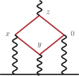
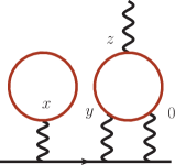
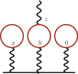
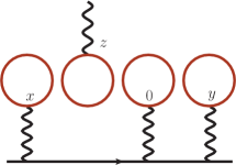
Figure 1: Five Wick-contraction topologies that are necessary for the calculation of $a_{\mu}^{\rm hlbl}$ as listed in Table 1. For each diagram, nontrivial permutations of the four quark-photon vertices yield the number of contractions listed in that table. The two diagrams in the first line are the dominant ones and the other three vanish in the SU$(3)_{\rm f}$ limit.

One can compute the light-by-light scattering contribution to the $g-2$ of the muon in position space by performing the integrals

$$a_{\mu}^{\rm hlbl}=\frac{m_{\mu}e^{6}}{3}\int d^{4}y\int d^{4}x\;\mathcal{\bar{L}}_{[\rho,\sigma];\mu\nu\lambda}(x,y)\;i\widehat{\Pi}_{\rho;\mu\nu\lambda\sigma}(x,y),$$ (1)

where $\mathcal{\bar{L}}$ is a QED kernel and $i\widehat{\Pi}$ is a spatial moment of the connected Euclidean four-point function in QCD,

$$i\widehat{\Pi}_{\rho;\mu\nu\lambda\sigma}(x,y) = -\int d^{4}z\,z_{\rho}\,\widetilde{\Pi}_{\mu\nu\sigma\lambda}(x,y,z),$$ (2)

$$\widetilde{\Pi}_{\mu\nu\sigma\lambda}(x,y,z) \equiv \Big{\langle}\,j_{\mu}(x)\,j_{\nu}(y)\,j_{\sigma}(z)\,j_{\lambda}(0)\Big{\rangle}_{\rm QCD}\,,$$ (3)

with $j_{\mu}(x)$ the hadronic component of the electromagnetic current

$$j_{\mu}(x)=\frac{2}{3}(\overline{u}\gamma_{\mu}u)(x)-\frac{1}{3}(\overline{d}\gamma_{\mu}d)(x)-\frac{1}{3}(\overline{s}\gamma_{\mu}s)(x)\,.$$ (4)

The QCD correlation function consists of all the various ways one can contract four vector currents, as shown in Fig. 1, all of which are “disconnected” except for the fully-connected contribution. At the flavor-symmetric point, only the upper two topologies contribute. Away from this point it is expected, from large-$N_{c}$ arguments as well as from numerical evidence by the RBC/UKQCD collaboration Blum et al. (2017), that the remaining topologies are suppressed. The number of contractions for each topology is given in Table 1.

	conn	$2+2$	$3+1$	$2+1+1$	$1+1+1+1$
$m_{l}\neq m_{s}$	6	3	8	6	1
$m_{l}=m_{s}$	6	3	0	0	0

Table 1: Number of contractions needed for each type of diagram in Fig. 1.

More information on the infinite-volume QED kernel $\mathcal{\bar{L}}(x,y)$ can be found in Asmussen et al. (2020). We make use of $O(4)$ symmetry to simplify the integral further,

$$a_{\mu}^{\rm hlbl}=\int_{0}^{\infty}d|y|\,f(|y|),$$ (5)

where in the starting representation (1),

$$f(|y|)=\frac{m_{\mu}e^{6}}{3}2\pi^{2}|y|^{3}\int d^{4}x\;\mathcal{\bar{L}}_{[\rho,\sigma];\mu\nu\lambda}(x,y)\;i\widehat{\Pi}_{\rho;\mu\nu\lambda\sigma}(x,y).$$ (6)

We will often display this integrand and always denote it by $f(|y|)$, even though in practice we employ modified representations of $a_{\mu}^{\rm hlbl}$. One type of modification concerns the kernel $\mathcal{\bar{L}}_{[\rho,\sigma];\mu\nu\lambda}(x,y)$. Various subtraction terms to the kernel have been proposed to beneficially change the shape of the integrand Blum et al. (2017); Asmussen et al. (2019b) without changing the resulting integral. The importance of performing such subtractions cannot be understated as the unsubtracted kernel is poorly suited for practical lattice simulations due to being too peaked at short distances.

Here we make extensive use of a new subtraction scheme for the QED kernel Asmussen et al. (2019b),

$$\mathcal{\bar{L}}^{(\Lambda)}_{[\rho,\sigma];\mu\nu\lambda}(x,y)= \mathcal{\bar{L}}_{[\rho,\sigma];\mu\nu\lambda}(x,y)$$ (7)

$$-\partial_{\mu}^{(x)}(x_{\alpha}e^{-\Lambda m_{\mu}^{2}x^{2}/2})\mathcal{\bar{L}}_{[\rho,\sigma];\alpha\nu\lambda}(0,y)$$

$$-\partial_{\nu}^{(y)}(y_{\alpha}e^{-\Lambda m_{\mu}^{2}y^{2}/2})\mathcal{\bar{L}}_{[\rho,\sigma];\mu\alpha\lambda}(x,0),$$

where $\Lambda$ is an arbitrary, tuneable, dimensionless free parameter. When $\Lambda=0$ we have the $\mathcal{\bar{L}}^{(2)}$ kernel of Asmussen et al. (2020) and as $\Lambda\rightarrow\infty$ we recover the unsubtracted $\mathcal{\bar{L}}^{(0)}$. The benefit of such a choice of kernel is that we are able to tune the shape of the integrand to reduce the long-distance effects while still preserving the beneficial properties of short-distance subtractions. An investigation of this kernel with the infinite-volume lepton loop is presented in Appendix B.

In this section we will write the formulae for obtaining $a_{\mu}^{\rm hlbl}$ in terms of continuous integrals. The lattice, however, is discrete so we can only approximate these integrals with finite sums,

$$\int d^{4}x\approx a^{4}\sum_{t/a=-N_{t}/2}^{N_{t}/2-1}\>\>\sum_{z/a=-N_{z}/2}^{N_{z}/2-1}\>\>\sum_{y/a=-N_{y}/2}^{N_{y}/2-1}\>\>\sum_{x/a=-N_{x}/2}^{N_{x}/2-1},$$ (8)

where $a$ is the lattice spacing and $N_{\mu}=L_{\mu}/a$. In Eq. (2), we set $z_{\rho}=L/2\rightarrow 0$ to accommodate the discontinuity when it changes sign. The integral of $f(|y|)$ with respect to $|y|$ can be performed with the trapezoid rule and in practice we will average over equivalent values of $f(|y|)$ to both increase statistical precision and reduce computational cost. Later on in the analysis we will show results for the partially-integrated value of $a_{\mu}$,

$$a_{\mu}(|y|_{\text{max}})=\int_{0}^{|y|_{\text{max}}}d|y|f(|y|)$$ (9)

with the hope that we will see a plateau at large-enough $|y|_{\text{max}}$, indicating that our integral has saturated.

In the following three subsections we will discuss two methods to compute the connected contribution: the first, Method 1, is a direct calculation of the three pairs of connected Wick contractions; the second, Method 2, uses rearrangements of the integrand expressed in terms of only one pair of Wick contraction to make the calculation cheaper. We will then give the methodology used for the calculation of the disconnected contribution, which also uses some rearrangements in the integrand.

II.1 Connected contribution (Method 1)

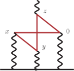
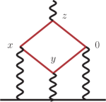
Figure 2: Wick contractions for the connected contribution. Each diagram represents two contractions with quark flow in opposite directions.

The Wick contractions for the connected contribution are shown in Fig. 2. With four local vector currents, the four-point correlation function can be written as

$$\widetilde{\Pi}^{\rm conn}_{\mu\nu\sigma\lambda}(x,y,z)=\frac{18}{81}Z_{V}^{4}\left(\widetilde{\Pi}_{\mu\nu\sigma\lambda}^{(1)}(x,y,z)+\widetilde{\Pi}_{\mu\nu\sigma\lambda}^{(2)}(x,y,z)+\widetilde{\Pi}_{\mu\nu\sigma\lambda}^{(3)}(x,y,z)\right)\,,$$ (10)

where $Z_{V}$ is the renormalization factor of the vector current and each term represents one diagram in Fig. 2, i.e. a pair of Wick contractions. We will use the $Z_{V}$ values from Gérardin et al. (2019b) without the $O(a)$-improvement terms proportional to quark mass combinations. The value $18/81$ is the necessary charge factor for the degenerate light and strange quarks. Writing the $\widetilde{\Pi}^{(1,2,3)}$s in terms of propagators yields

$$\widetilde{\Pi}_{\mu\nu\sigma\lambda}^{(1)}(x,y,z)= -2\text{Re}\left\langle\,\hbox{\rm Tr}\left[S(0,x)\gamma_{\mu}S(x,y)\gamma_{\nu}S(y,z)\gamma_{\sigma}S(z,0)\gamma_{\lambda}\right]\right\rangle_{U},$$ (11)

$$\widetilde{\Pi}_{\mu\nu\sigma\lambda}^{(2)}(x,y,z)= -2\text{Re}\left\langle\,\hbox{\rm Tr}\left[S(0,y)\gamma_{\nu}S(y,z)\gamma_{\sigma}S(z,x)\gamma_{\mu}S(x,0)\gamma_{\lambda}\right]\right\rangle_{U},$$

$$\widetilde{\Pi}_{\mu\nu\sigma\lambda}^{(3)}(x,y,z)= -2\text{Re}\left\langle\,\hbox{\rm Tr}\left[S(0,y)\gamma_{\nu}S(y,x)\gamma_{\mu}S(x,z)\gamma_{\sigma}S(z,0)\gamma_{\lambda}\right]\right\rangle_{U},$$

where $S(x,y)$ is the quark propagator with sink at $x$ and source at $y$ and $\langle\cdots\rangle_{U}$ is the expectation value over gauge configurations. The trace is over both Dirac and color indices. In Method 1, the six contractions are computed explicitly and we choose the direction $y/a\propto(1,1,1,1)$. In this method, we first compute the point-to-all propagator $S(\cdot,0)$ and the six sequential propagators using the fields $z_{[\rho}\gamma_{\sigma]}S(z,0)$ as sources (the anti-symmetrization of the indices $\rho$ and $\sigma$ is imposed by the symmetries of the QED kernel). Then, for each value of $|y|$ used to sample the integrand in Eq. (5), we compute the point-to-all propagator $S(\cdot,y)$ and the six sequential propagators using the fields $z_{[\rho}\gamma_{\sigma]}S(z,y)$ as sources. Therefore, for $N$ evaluations of the integrand, we need $7(N+1)$ propagator inversions. In our set-up all currents are local except for the one at $x$, which will be either local or the point-split, the latter implying a suitable modification of Eq. (11).

In practice, since we are (mostly) using open-boundary conditions in the time direction, the origin is located somewhere near the middle time-slice and randomly distributed in the spatial volume. We also average over the 16 combinations $y/a=(\pm n,\pm n,\pm n,\pm n)$ to increase statistics.

II.2 Connected contribution (Method 2)

The idea for Method 2 is simple: we pick a reference diagram that is easiest to compute and use a change of variables in the integrals to relate the other diagrams to this reference. Here, we pick the diagram that does not have a propagator from the origin to $y$, or from $z$ to $x$ (the leftmost of Fig. 2). Such a choice avoids the extra inversions required for the sequential sources as we discussed in Method 1. Simplistically, for two samples of a single $|y|$ (i.e. $+y$ and $-y$) we only need two point-to-all propagators. In fact, we can do much better than this if we keep propagators in memory so that they can be reused.

The diagrams $\widetilde{\Pi}^{(2)}$ and $\widetilde{\Pi}^{(3)}$ are related to $\widetilde{\Pi}^{(1)}$ by applying symmetries to Eq. (11): Euclidean-space translations and inversions, along with cyclicity of the trace Asmussen et al. (2019b, 2020). This leads to our master formula for Method 2:

$$\begin{gathered}a_{\mu}^{\rm conn}=-\frac{18}{81}Z_{\rm V}^{4}\frac{m_{\mu}e^{6}}{3}2\pi^{2}\int d|y||y|^{3}\;\int d^{4}x\\ \bigg{(}(\mathcal{\bar{L}}^{(\Lambda)}_{[\rho,\sigma];\mu\nu\lambda}(x,y)+\mathcal{\bar{L}}^{(\Lambda)}_{[\rho,\sigma];\nu\mu\lambda}(y,x)-\mathcal{\bar{L}}^{(\Lambda)}_{[\rho,\sigma];\lambda\nu\mu}(x,x-y))\int d^{4}z\>z_{\rho}\widetilde{\Pi}^{(1)}_{\mu\nu\sigma\lambda}(x,y,z)\\ +\mathcal{\bar{L}}^{(\Lambda)}_{[\rho,\sigma];\lambda\nu\mu}(x,x-y)x_{\rho}\int d^{4}z\>\widetilde{\Pi}^{(1)}_{\mu\nu\sigma\lambda}(x,y,z)\bigg{)}.\end{gathered}$$ (12)

In infinite volume, the integral is equal to the result of Method 1, but the integrand $f(|y|)$ will generally be different. As a result, the systematic effects in Method 2 will be different from Method 1.

We invert point-source propagators along the line $(n,n,n,3n+t_{\text{min}}/a)$, and what we call $|y|$ will be the difference between these points; here the integer $n$ ranges from 0 to $N_{i}/2$. The closest source position in time ($t_{\text{min}}$) is chosen to be suitably away from our (usually) open temporal boundary, ideally $m_{\pi}t_{\text{min}}>4$ and $m_{\pi}(L_{t}-t_{\text{max}})>4$. This line of propagator sources was chosen as we typically have a large anisotropy in the temporal direction, allowing us to achieve sizeable values of $|y|$.

In our implementation, we keep all $N_{i}/2$ of the propagators in memory and perform the integrals for every possible $y$ and origin, so for $N$ propagator inversions we have $N(N-1)$ samples distributed among the different values of non-zero $|y|$. To further boost statistics we will also average other directions that give the same $|y|$, e.g. $y/a=(\pm n,\pm n,\pm n,t_{\text{max}}/a-3n)$.

II.3 Disconnected contribution

The disconnected contribution can be computed from the two-point contraction

$$\Pi_{\mu\nu}(x,y)=-\text{Re}\left(\text{Tr}[S(y,x)\gamma_{\mu}S(x,y)\gamma_{\nu}]\right).$$ (13)

An important point to note is that $\Pi_{\mu\nu}$ has a vacuum expectation value (VeV) that must be subtracted to ensure that the two “disconnected” quark loops are still connected by gluons. To this end, we define

$$\hat{\Pi}_{\mu\nu}(x,y)=\Pi_{\mu\nu}(x,y)-\langle\Pi_{\mu\nu}(x,y)\rangle_{U},$$ (14)

and use this to compute the $2+2$ quark-disconnected contribution to $a_{\mu}^{\rm hlbl}$,

$$a_{\mu}^{\rm disc}= -\frac{36}{81}Z_{\rm V}^{4}\frac{m_{\mu}e^{6}}{3}2\pi^{2}\int d|y||y|^{3}\int d^{4}x$$ (15)

$$\biggl{\langle} (\mathcal{\bar{L}}^{(\Lambda)}_{[\rho,\sigma];\mu\nu\lambda}(x,y)+\mathcal{\bar{L}}^{(\Lambda)}_{[\rho,\sigma];\nu\mu\lambda}(y,x))\hat{\Pi}_{\mu\lambda}(x,0)\int d^{4}z\>z_{\rho}\hat{\Pi}_{\sigma\nu}(z,y)$$

$$+\mathcal{\bar{L}}^{(\Lambda)}_{[\rho,\sigma];\mu\nu\lambda}(x,y)\hat{\Pi}_{\mu\nu}(x,y)\int d^{4}z\>z_{\rho}\hat{\Pi}_{\sigma\lambda}(z,0)\biggr{\rangle}_{U}.$$

In our implementation we compute a grid of point-source propagators from some $t_{\text{min}}$ to $t_{\text{max}}$ wrapping completely around the spatial directions alternating between $(2n,2n,2n,6m+t_{\text{min}}/a)$ and $(2n+1,2n+1,2n+1,6m+3+t_{\text{min}}/a)$ where $n$ and $m$ take values between $0$ and $N_{i}/2-1$, and $0$ and $(t_{\text{max}}-t_{\text{min}})/(6a)$ respectively.

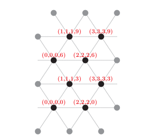
Figure 3: Illustration of the grid of propagators used in the toy example given in the text. Filled circles indicate sites that lie on the lattice, gray circles are ones accessible through periodicity and the dashed lines indicate lines along our preferred directions $(1,1,1,3)$ and $(2,2,2,0)$.

Giving a toy example; for a $4^{3}\times 12$ periodic lattice we would invert point-source propagators at $(0,0,0,0),(2,2,2,0),(1,1,1,3),(3,3,3,3),(0,0,0,6),(2,2,2,6),(1,1,1,9),$ and $(3,3,3,9)$. This is illustrated in Fig. 3. We then compute the two-point contraction of Eq. (13) for each of these sources and keep it in memory. We then perform a doubly-nested loop over all of the source positions, where we only integrate combinations of two-point contractions where our $y$ lies in a direction we like, e.g. along the directions $(1,1,1,3)$ and $(2,2,2,0)$. The results of the $z$ and $x$ integrations are saved to disk, the VeV is subtracted, and the final contraction of indices is performed offline in the analysis.

The benefit of such a method over calculating each separate $|y|$ individually is the quadratic growth of equivalent combinations of $|y|$ that are available as the number of source fields grows. For our $4^{3}\times 12$ example we have $6$ values of equivalent $|y|$ per source position. It would be impractical to perform this calculation without exploiting this fact. We find it is beneficial to truncate the $x$-integral in our set-up to avoid negligible, noisy contributions at large distances. As our kernels are computed on-the-fly this is also useful as a computer-time saving measure as it reduces the number of QED kernel calls. We truncate the integral over $x$ to points that lie within a maximum distance [$(r/a)^{2}=81,81,121,169$ for our coarsest to finest ensembles respectively] from the origin or from $y$, while we do not truncate the $z$-integral. Although these truncations differ in physical volume, the ensembles H101 and H200 were tested for smaller and larger values of $(r/a)^{2}$ on a subset of our data and even smaller values of $(r/a)^{2}$ than used here, for example $49$ and $64$ for the ensemble H101, were found to be consistent.

To reiterate, in our full calculation we do not perform the integrals for all possible $y$-vectors, as there are many that we expect to have bad finite-volume or discretization effects. For instance, in the toy example we could calculate $f(|y|)$ for the $y$-vector $y/a=(0,0,0,6)$, but this would have significant cut-off effects. Typically, we filter-out about $\approx 80\%$ of the possible $y$-vectors and keep only (the modulus of) those parallel to $(1,1,1,3)$, $(2,2,2,0)$, and occasionally $(1,1,1,1)$.

III Lattice parameters and properties of SU$(3)_{\rm f}$-symmetric QCD

Calculations have been performed on lattice ensembles provided by the Coordinated Lattice Simulations (CLS) initiative Bruno et al. (2015), which have been generated using three flavors of non-perturbatively $O(a)$-improved Wilson-clover fermions and with the tree-level $O(a^{2})$-improved Lüscher-Weisz (Symanzik) gauge action. In particular, we consider only those with SU$(3)_{\rm f}$-symmetry. On these ensembles, the mass of the octet of light pseudoscalar mesons is approximately 420 MeV. These ensembles are summarized in Table 2 and in Fig. 4: there are four lattice spacings, as well as two pairs of ensembles that differ only by their volume.

Label	$\beta$	$\kappa$	size	bdy. cond.	$a$ (fm)	$m_{\pi,K,\eta}$ (MeV)	$m_{\pi}L$
U103	3.40	0.13675962	$24^{3}\times 128$	open	0.08636(98)(40)	415(5)	4.4
H101	3.40	0.13675962	$32^{3}\times 96$	open	0.08636(98)(40)	418(5)	5.9
B450	3.46	0.13689	$32^{3}\times 64$	periodic	0.07634(92)(31)	417(5)	5.2
H200	3.55	0.137	$32^{3}\times 96$	open	0.06426(74)(17)	421(5)	4.4
N202	3.55	0.137	$48^{3}\times 128$	open	0.06426(74)(17)	412(5)	6.4
N300	3.70	0.137	$48^{3}\times 128$	open	0.04981(56)(10)	421(5)	5.1

Table 2: Lattice ensembles with SU$(3)_{\rm f}$-symmetry used in this work. Each ensemble is parametrized by the gauge coupling parameter $\beta$, the quark hopping parameter $\kappa$, the lattice size, and the temporal boundary condition. The lattice spacing $a$ was determined in Ref. Bruno et al. (2017).

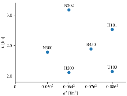
Figure 4: Spatial extent $L$ and lattice spacing $a$ for the ensembles with SU$(3)_{\rm f}$-symmetry used in this work.

III.1 The $\text{SU}(3)_{\rm f}$ meson spectrum

At long distances, the leading contributions to the four-point correlator emanate from the lowest-lying mesons. Clearly, the degenerate $\pi^{0}$ and $\eta$-pole contributions dominate at the longest distances. However, at intermediate distances the contributions from heavier states, including resonances in the two-pseudoscalar channel, may also play a significant rôle. Especially since in our calculation at the SU$(3)_{\rm f}$-point the pseudoscalar mesons are not appreciably light compared to the other mesons. Therefore, we present results from a limited spectroscopic study of the low-lying meson spectrum in all relevant channels with total angular momentum $J\leq 1$.

Only charge-conjugation-even ($C$-even) mesons can couple to two electromagnetic currents and thus contribute in exchange diagrams to the four-point function. However, from the Wick-contraction structure, one can view Method 2 as using charged vector currents (see Appendix A) and it is possible to couple a $C$-odd state to two of them. Therefore, the integrand for Method 2 can receive contributions from $C$-odd mesons such as the rho Asmussen et al. (2019b). For that reason, we also inspect the spectrum of $C$-odd mesons, even if their contributions to $a_{\mu}^{\rm hlbl}$ must vanish in the infinite-volume limit once all integrals are performed.

Our dedicated spectroscopy calculation is performed on the ensemble H101. This made use of the distillation framework Peardon et al. (2009) (for the connected hadron two-point functions) and its stochastic formulation Morningstar et al. (2011), which was essential for efficiently computing the disconnected hadron two-point functions needed in the singlet sector. However, we have only used smeared quark bilinears as interpolating operators, and the lack of non-local multimeson-like interpolators means that this calculation should not generally be considered as a robust determination of the spectrum. This analysis precludes the use of finite-volume quantization conditions; therefore, only the approximate locations of resonances can be found, provided that they are narrow. Nevertheless, since we compute diagonal correlators, the effective masses taken at any Euclidean time provide an upper bound on the ground-state energy in a given channel. This observation is particularly useful in the flavor-singlet $0^{++}$ channel, which turns out to admit a stable ground-state meson. Such a stable scalar meson has been found previously Briceno et al. (2017) in a lattice calculation at a similar pion mass, though not at an SU(3)_f-symmetric point.

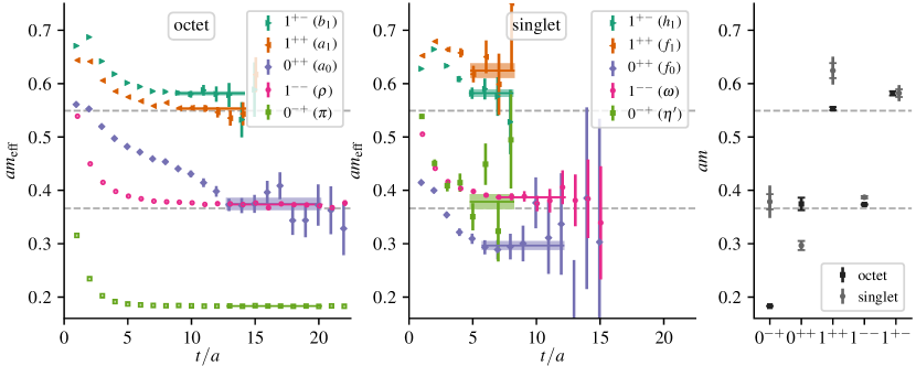
Figure 5: The meson spectrum of ensemble H101. Effective masses are shown for each channel in the flavor octet (left) and singlet (center) sectors, along with bands indicating the plateau fits. Note that in many cases (in particular the octet pseudoscalar and vector channels), the error bar is smaller than the plotted symbol. Fitted masses are shown in the right panel; the outer error bars include an estimate of systematic uncertainty obtained by shifting the plateau fit range. Horizontal dashed lines indicate thresholds at twice and three times the octet pseudoscalar mass.

$J^{PC}$	octet		singlet
$0^{-+}$	$\pi$	418(1)(0)	$\eta^{\prime}$	865(32)(61)
$0^{++}$	$a_{0}$	856(27)(12)	$f_{0}$	678(20)(10)
$1^{++}$	$a_{1}$	1264(7)(9)	$f_{1}$	1427(32)(50)
$1^{--}$	$\rho$	853(2)(1)	$\omega$	884(5)(3)
$1^{+-}$	$b_{1}$	1329(9)(3)	$h_{1}$	1330(16)(30)

Table 3: Estimated meson masses in MeV from ensemble H101. The first uncertainty is statistical and the second was determined by varying the plateau fit range. The scale-setting uncertainty has not been included.

Results are shown in Fig. 5 and summarized in Table 3. Note that since the signal in the flavor-singlet sector is much worse, the plateau fits had to be done at relatively short time separations, so that the shown uncertainty on the mass may be an underestimate. In addition, the plateau for the flavor-octet scalar is relatively poor, which might be due to its coupling to two octet pseudoscalars in S-wave and the plateau’s proximity to the corresponding threshold. In the case of a mis-identified plateau, the true ground-state energy would be lower, since the effective masses shown here are expected to approach the ground-state energy from above.

For the flavor-octet sector, after the $\pi^{0}$, the next-longest-distance meson-exchange contributions in the integrand for $a_{\mu}^{\rm hlbl}$ come from the $a_{0}$ and (for the Method 2 integrand) the $\rho$, both of which sit near $2m_{\pi}$. For the flavor-singlet sector, the three corresponding mesons are also the lightest, although the ordering is different, with the $f_{0}$ (or $\sigma$) being a bound state with mass near 680 MeV and the $\eta^{\prime}$ mass sitting higher, somewhere near $2m_{\pi}$. For the disconnected diagrams, which receive the difference between contributions from the exchanges of singlet and octet mesons (see section IV.1), the pseudoscalars will provide the longest-distance contribution but we should also expect a significant contribution from scalars. The difference between the octet and singlet vector meson masses is very small; if the same holds for their form factors, then their combined contribution to the integrand will be negligible.

III.2 Pion-pole and $\eta$-pole contributions to $a_{\mu}^{\rm hlbl}$

In Ref. Gérardin et al. (2019a) a model independent parametrization of the pion TFF has been obtained on the same set of lattice ensembles as used in this work. These results can be used to compute the pion-pole contribution, $a_{\mu}^{\mathrm{hlbl};\pi^{0}}$, at the SU$(3)_{\rm f}$-symmetric point in the continuum limit. This result will be used in Section VII.3 to obtain a rough estimate of $a_{\mu}^{\rm hlbl}$ at the physical pion mass. More importantly, in Sections V.1, V.2, and VI, a vector meson dominance (VMD) parametrization of the TFF will be used to estimate the finite-size corrections to our lattice data at the symmetric point. For this purpose, we have performed a new fit to the data from Gérardin et al. (2019a) assuming a VMD parametrization, where we have restricted the fit to the singly-virtual case where the model provides a good description of our data. The fit parameters used in this work are collected in Table 4.

In Gérardin et al. (2019a), two strategies have been used to extract the pion TFF, and the corresponding results for the pion-pole contribution are displayed in Fig. 6 for two different discretizations of the 3-point correlation function (see Gérardin et al. (2019a) for details). In the first strategy, the TFF was computed on each lattice ensemble separately. This allowed us to determine the pion-pole contribution for different values of the pion mass and lattice spacing. The physical value was then obtained by a combined chiral-continuum extrapolation of $a_{\mu}^{\mathrm{hlbl};\pi^{0}}$. We have repeated this analysis but now restrict the fit to only the ensembles included in this study. Here we use the pion mass of the given ensemble (instead of the physical one as done in Gérardin et al. (2019a)) in the weight functions that appear in Eq. (74) of Gérardin et al. (2019a). This leads to the result (1) of Fig. 6.

In the second strategy, the pion TFF was directly extrapolated to the physical point using a global fit that includes several ensembles including, and away from, the SU$(3)_{\rm f}$-point. From the resulting fit parameters, we can extract the pion TFF in the continuum limit at a pion mass of 420 MeV. Using this result in Eq. (74) of Gérardin et al. (2019a), we obtain the grey point of Fig. 6, which we find to be in very good agreement with the first estimate.

Label	${\cal F}_{\pi^{0}\gamma\gamma}(0,0)$$\,[{\rm GeV}^{-1}]$	$M_{V}$ [MeV]
H101	0.237(5)	921(13)
B450	0.230(5)	942(25)
H200	0.219(6)	979(26)
N202	0.227(5)	952(15)
N300	0.214(5)	1001(23)

Table 4: The VMD fit parameters of the $\pi^{0}$ transition form factor.

The second strategy has the advantage of using an expanded set of ensembles (15 in total) to determine the TFF,

$$a_{\mu}^{\mathrm{hlbl};\pi^{0}}=21.0(1.2)\times 10^{-11}\qquad(\textrm{SU$(3)_{\rm f}$ point})$$ (16)

at the SU$(3)_{\rm f}$-point which is to be compared to the physical-pion value

$$a_{\mu}^{\mathrm{hlbl};\pi^{0}}=59.7(3.6)\times 10^{-11}\qquad(\textrm{physical point}).$$ (17)

Unsurprisingly, we observe a strong dependence on the pion mass. The smaller pion contribution in Eq. (16) compared with (17) is due roughly in equal parts to the heavier pion mass and to the reduced coupling to photons, as can be seen by comparing the entries in Table 4 to the physical value, ${\cal F}_{\pi^{0}\gamma\gamma}(0,0)\approx 0.274\,{\rm GeV}^{-1}$.

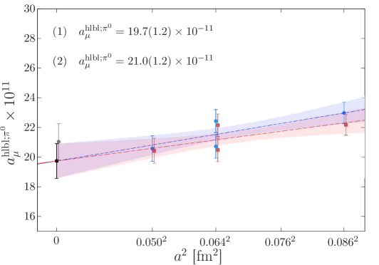
Figure 6: The pion-pole contribution to $a_{\mu}^{\rm hlbl}$ at the SU(3)_f symmetric point with a pion mass of 420 MeV. Blue and red points correspond to two different discretizations of the 3-pt correlation function. The results (1) and (2) are explained in the main text.

At the SU$(3)_{\rm f}$-symmetric point, the $\eta$ is mass-degenerate with the pion, $m_{\eta}\simeq 420\,$MeV, and contributes exactly $1/3$ of the $\pi^{0}$ exchange to $a_{\mu}^{\rm hlbl}$, i.e.

$$a_{\mu}^{\rm hlbl;\eta}=(7.0\pm 0.4)\times 10^{-11}\qquad(\textrm{SU$(3)_{\rm f}$-point}).$$ (18)

A lattice calculation at the physical point for this contribution is not yet available, but the most recent estimate, which comes from Canterbury approximants Masjuan and Sanchez-Puertas (2017); Aoyama et al. (2020), is $a_{\mu}^{\rm hlbl,\eta,{\rm phys}}=16.3\times 10^{-11}$. This comparison shows that at the physical point the $\eta$ gives a much larger contribution to $a_{\mu}^{\rm hlbl}$ than at the SU$(3)_{\rm f}$-symmetric point, in spite of being heavier. This can be traced back to its much larger coupling to two photons,

$${\cal F}_{\eta\gamma\gamma}(0,0)[{\rm GeV}^{-1}]\simeq\left\{\begin{array}[]{ll}0.12&\textrm{SU$(3)_{\rm f}$ point},\\ 0.27&\textrm{physical point}.\end{array}\right.$$ (19)

IV Hadronic models vs.  the lattice integrand $f(|y|)$

In subsection IV.1, we state the theoretical predictions for the integrand $f(|y|)$ corresponding to the quark-connected diagrams in Method 1 and Method 2, as well as for the disconnected diagram. Then, in subsection IV.2, we compare the lattice $|y|$-integrand obtained by Method 1 for the quark-connected contribution to hadronic model predictions. For this purpose, we will focus on the ensembles N202 and H200. N202 has the largest physical volume ($L=3.08$ fm) of all ensembles considered in this work, and H200 (with $L=2.06$ fm) differs only by its comparatively smaller volume. Since these only differ by their volume, they allow us to test our understanding of finite-volume effects. Finally, a comparison of the theory predictions for the integrand of the quark-disconnected contributions to the corresponding lattice data is made in subsection IV.3.

IV.1 Predictions for the integrand

In order to gain some insight into the various contributions to the quantity $a_{\mu}^{\rm hlbl}$, we will compare predictions for the pseudoscalar exchanges as well as the contribution from a constituent-quark loop, and a charged-pseudoscalar loop, to the lattice data. Here, we provide some details as to how these predictions are obtained. Expressions for the amplitudes $i\widehat{\Pi}_{\rho;\mu\nu\lambda\sigma}$ calculated with a fermion loop, a charged-pion loop, or with the pseudoscalar exchange can be found in Asmussen et al. (2018, 2020). In QCD with exact SU(3)_f-symmetry, the $\eta$ contribution to $a_{\mu}^{\rm hlbl}$ is always one third of the contribution of the $\pi^{0}$.

The flavor structure of single-meson exchanges in the different Wick-contraction topologies of four-point functions was discussed in detail in Ref. Gérardin et al. (2018), including the case of $N_{\rm f}=3$ QCD. The quark-connected diagrams receive contributions only from flavor-octet mesons, enhanced by a factor of three. This is compensated by the quark-disconnected diagrams, which contain the differences between the flavor-singlet and twice the flavor-octet meson contributions. In the large-$N_{c}$ limit, the singlet and octet contributions to the disconnected diagrams will cancel as their spectra becomes the same. For QCD, this degeneracy is most strongly broken in the pseudoscalar sector, where the octet’s mass is far below the singlet’s.

To interpret the integrand in Method 2, one needs a mapping of individual quark-level Wick contractions onto meson-exchange diagrams Asmussen et al. (2019b) (see Appendix A for a derivation based on partially quenched chiral perturbation theory). It turns out that $\widetilde{\Pi}^{(1)}_{\mu\nu\sigma\lambda}(x,y,z)$ does not contain the meson-exchange diagram in which the $\pi^{0}$ and $\eta$ propagate between the pair of vertices $(0,y)$ and $(x,z)$. Also, the normalization of the two other $(\pi^{0},\eta)$-exchange diagrams is such that $\widetilde{\Pi}^{\rm conn}_{\mu\nu\sigma\lambda}$ contains the same $(\pi^{0},\eta)$ contribution as $\widetilde{\Pi}_{\mu\nu\sigma\lambda}$, enhanced (in the present SU(3)_f case) by the charge factor three.

In addition, we need the mapping of individual quark-level disconnected diagrams onto meson-exchange diagrams. Here it turns out that there is a one-to-one mapping between a given quark-level diagram and a meson-exchange diagram. For instance, take a quark-level diagram, consisting of two quark loops each containing two vectorial vertices; each quark loop thus defines a pair of vertices. Such a diagram is in one-to-one correspondence with the diagram in which the meson is exchanged between the two pairs of vertices. For octet mesons, the latter diagram has a weight of $-2$ relative to its normalization in the full HLbL amplitude. For singlet mesons, this relative weight factor is simply unity.

The short-distance contribution to $a_{\mu}^{\rm hlbl}$ is sometimes modelled by a constituent-quark loop. This corresponds to an effective degree of freedom, and the mass assigned to the ‘constituent quark’ is typically on the order of 300 MeV Bijnens et al. (1996). In the following sub-section, we will address the question “to what extent does such a contribution describe the short-distance part of the $|y|$ integrand?”. In this case, the Wick contractions and weight factors of the constituent quark simply correspond to those of the fundamental quark degrees of freedom.

We have computed the charged pion and kaon loop contributions in the framework of scalar QED Asmussen et al. (2019b, 2020). The contribution of these loops to the set of quark-connected contractions and their contribution to the set of quark-disconnected contractions add up coherently, the latter being twice as large as the former. This result can again be derived in partially-quenched perturbation theory. While the $(\pi^{0},\eta)$ exchange contribution to the full $a_{\mu}^{\rm hlbl}$ is three times smaller than its contribution to $a_{\mu}^{\rm conn}$, the charged-pseudoscalar loop contribution is three times larger. The charged-pseudoscalar loop’s contribution might seem negligible in comparison to the integrand of the quark-connected, but it need not be negligible in the full integrand.

IV.2 Lattice connected contribution

Fig. 7 displays the integrand obtained with Method 1 and $\Lambda=0.16$. It is compared to the integrand for the exchange of the $(\pi^{0},\eta)$ mesons with a VMD TFF and using the parameters of Table 4. Beyond 1.5 fm, the prediction is consistent with the lattice data, albeit within large relative errors. Between 0.8 fm and 1.4 fm, the lattice data lie noticeably below the pseudoscalar-octet exchange prediction.

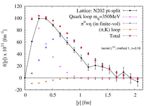
Figure 7: Integrand for the connected contribution on ensemble N202 using Method 1 with $\Lambda=0.16$. The lattice data use a point-split current at $x$. The integrand is compared to the prediction for the exchange of the $\pi^{0}$ and $\eta$ mesons with a VMD transition form factor, which is expected to provide a good approximation to the tail. In addition, an attempt to describe the short-distance contribution with a constituent-quark loop with a quark mass of 350 MeV is made.

At distances up to 0.8 fm, one would certainly not expect the pseudoscalar-octet exchange to saturate the integrand. We have attempted to model the higher-energy contributions using a constituent-quark loop, displayed in Fig. 7. For a constituent-quark mass of 350 MeV, the sum of this contribution and the pseudoscalar-octet exchange provides a good description of the maximum height of the integrand. At distances $|y|\lesssim 0.4$ fm, one must expect large cutoff effects on the lattice integrand, as the separation of sources becomes comparable to our lattice spacing. This interpretation is confirmed by comparing the integrand to the one obtained using exclusively the local current, as in the left panel of Fig. 8, where a sizeable difference is visible up to about 0.4 fm. An interesting observation is that upon adding the constituent-quark loop to the pseudoscalar-octet exchange the result does not improve the agreement with the lattice data in the region $0.8{\rm\,fm}<|y|<1.4{\rm\,fm}$. A clear excess remains in the prediction; we currently do not have a compelling explanation for this excess. The exchange of the lightest scalar-octet mesons ($a_{0}$ type) would have the right sign to explain the effect, since scalar-meson exchanges are known to contribute negatively to $a_{\mu}^{\rm hlbl}$. In the future, a calculation of the scalar contribution along the lines of Knecht et al. (2018) would be worthwhile to find out whether it accounts for this missing effect. The charged-pion loop is also expected to contribute negatively and we have studied this contribution in the scalar-QED framework in Asmussen et al. (2019b). We found the integrand to be negligible compared with the $\pi^{0}$ contribution beyond $|y|=0.6\,$fm, and introducing a vector form factor for the charged pion would likely only reduce the integrand further. It thus remains an open problem to understand the physics underlying the integrand for $|y|$ around 1 fm.

The effect of the finite volume on the lattice integrand is illustrated in Fig. 9. A clear effect is seen between the comparatively ‘small’ ensemble H200 and the ‘large’ N202, the former integrand lying below the latter. This finite-volume dependence matches in sign and typical size the volume dependence of the pseudoscalar-octet exchange contribution, as seen in the figure.

IV.3 Lattice disconnected contribution

Fig. 12 (later in the text) displays the disconnected integrand for several gauge ensembles. It is compared to the prediction of the $(\pi^{0},\eta)$ exchange, including its appropriate weight factor of $-2$ for the disconnected contribution, both in finite and infinite volume. The finite-volume effect predicted from the $(\pi^{0},\eta)$ exchange calculation is very small, and the lattice data from ensembles N202 and H200 confirms this expectation, at least at distances $|y|<0.9\,$fm, where the statistical errors allow for a meaningful comparison.

The main difference between the disconnected and the connected contributions is that for the disconnected the $(\pi^{0},\eta)$ exchange already provides a decent description of the lattice data for $|y|$ below 1 fm; in other words, we do not observe a large short-distance contribution. The $\eta^{\prime}$ and the $\sigma$ mesons being singlets, they contribute to the disconnected diagrams with the same weight factor as they would to the full HLbL amplitude Bijnens and Relefors (2016); Gérardin et al. (2018). In order to estimate the typical size of these heavy-meson contributions, we have computed the $\eta^{\prime}$ contribution under the following assumptions: The $\eta^{\prime}$ mass was set to 982 MeV, a value close to the result of our calculation on ensemble H101. Its coupling to two photons, ${\cal F}_{\eta^{\prime}\gamma\gamma}$, was assumed to be equal to its value at physical quark masses. The virtuality dependence of the transition form factor can be modelled with a VMD ansatz, with vector mass 952 MeV. Under these assumptions, the contribution is positive and sizeable (compared to the $(\pi^{0},\eta)$ exchange) up to $|y|=1.5\,$fm. In addition, we expect a significant contribution from the stable $\sigma$ meson, whose mass we have found to lie well below the $\pi\pi$ threshold. As a scalar, the $\sigma$ would contribute negatively and thus compensate to some extent the $\eta^{\prime}$ contribution. Again, a dedicated calculation in the framework of Knecht et al. (2018) would certainly be worthwhile. The estimate for the $\eta^{\prime}$ contribution displayed in Fig. 12 is only meant to be representative of one particular meson-exchange contribution, with other cancellations being expected.

V Results for the quark-connected contribution

V.1 Results from Method 1

The lattice results for the quark-connected contribution to $a_{\mu}^{\rm hlbl}$ using Method 1 have been generated along the direction $y/a\propto(1,1,1,1)$. We have used two different discretizations of the four-point correlation function: the vector current located at the site $x$ is either local or point-split (conserved), while the three other currents are always local. Our results are summarized in Table 5 and the integrand for the ensemble N202 (also presented in Sec. IV.2, Fig. 7) is shown on Fig. 8. The signal-to-noise ratio clearly deteriorates rapidly at large distances and we observe slightly better statistical precision when using a conserved vector current at $x$. Both discretizations give similar results, suggesting that there are small discretization effects present. In the end we will quote a final result with the fully-local discretization for a direct comparison with the results obtained using Method 2.

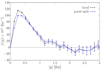
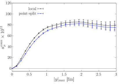
Figure 8: Results for the ensemble N202 using Method 1 with $\Lambda=0.16$. Black points use a local current at the site $x$ in Eq. (6) (which is our default approach) and blue points use a conserved current at $x$. Left: integrand $f(|y|)$ as a function of $|y|$. Right: integrated value of $a_{\mu}^{\rm conn}$ as a function of $|y|_{\rm max}$.

Although all the ensembles used in this work satisfy $m_{\pi}L>4$, we still expect significant finite size effects (FSEs) due to the pseudoscalar-pole contribution, which is the dominant contribution in model estimates of hadronic light-by-light scattering Prades et al. (2009), being a long-range phenomenon. Even with heavy pions $m_{\pi}\approx 400~{}$MeV, the tail extends beyond $|y|=2.5~{}\text{fm}$ Asmussen et al. (2020). A comparison of the integrand for the ensembles H200 and N202, which only differ by their physical volumes, is depicted on the left panel of Fig. 9. Assuming a VMD model for the TFF, the pseudoscalar contribution can be computed in both finite and infinite volume. For more information on the calculation of the TFF we refer the reader back to Sec. III.2; the parameters we use for modelling our data are summarized in Table 4 in that section.

To obtain our final estimate, the lattice data are integrated up to $|y|_{\rm cut}$ where the integrand is compatible with zero. For $|y|>|y|_{\rm cut}$, the tail is aproximated by the pseudoscalar-pole contribution in infinite volume. Finally, for $|y|<|y|_{\rm cut}$, the FSEs are estimated as the difference between the pseudoscalar-pole’s contribution computed in finite and infinite volume:

$$a_{\mu}^{\rm conn}=a_{\mu}^{\rm data}+a_{\mu}^{\rm tail}+a_{\mu}^{\rm FSE}\,.$$ (20)

A systematic error of 25% is attributed to both the tail extension and the FSE correction. Since the same VMD model is used in both cases, we treat these corrections as being fully correlated.

The value of $a_{\mu}^{\rm conn}$ as a function of $|y|_{\rm cut}$ is shown in the right panel of Fig. 9; we observe a nice plateau for values $|y|_{\rm cut}>1.2~{}$fm, suggesting that our systematic error estimate is quite conservative. Estimates of the finite-size corrections for each ensemble are summarized in Table 5 with their corresponding values of $|y|_{\rm cut}$. In particular, we note that the systematic error on the FSEs is always larger than the statistical precision, except for our largest ensemble N202.

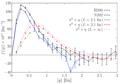
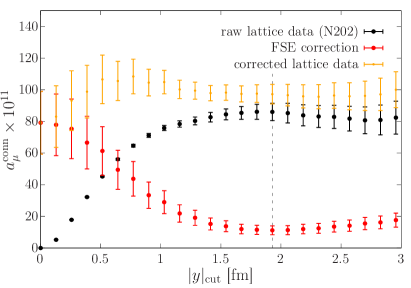
Figure 9: Study of FSEs for Method 1. Left: Integrand for the ensembles H200 and N202 with $m_{\pi}L=4.4$ and 6.4 respectively. Right: Value of $a_{\mu}^{\rm conn}$ for the ensemble N202 using the FSE correction prescription described in the text, as a function of $|y|_{\rm cut}$

Label	$|y|_{\rm cut}$ [fm]	$a_{\mu}^{\rm data}$	$a_{\mu}^{\rm FSE}$	$a_{\mu}^{\rm tail}$	$a_{\mu}^{\text{conn}}$
U103	1.55	69.0(2.2)	31.0	4.3	104.3(2.2)(8.8)
H101	1.73	71.6(2.9)	13.1	3.8	88.5(2.9)(4.2)
B450	1.68	72.9(3.8)	18.3	4.0	95.2(3.8)(5.6)
H200	1.54	71.1(2.8)	27.3	6.1	104.4(2.8)(8.4)
N202	1.93	85.5(4.5)	9.0	1.7	96.3(4.5)(2.7)
N300	1.59	79.2(4.2)	15.6	4.1	99.0(4.2)(4.9)

Table 5: Results for the connected contribution using Method 1 with four local vector currents using the decomposition given by Eq. (20). A $25\%$ systematic to the total correction is used.

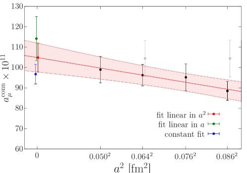
Figure 10: Continuum extrapolation of the connected contribution using Method 1. We perform a linear fit in $a^{2}$ (red), a linear fit in $a$ (green) or a constant fit (blue). The coarsest lattice spacing is excluded from the constant fit. Ensembles in grey have $m_{\pi}L<5$ and are not included in the fits and they have been shifted for clarity.

For the ensembles U103 and H200, with $m_{\pi}L<5$, we see very large FSE corrections, of the order of $50~{}\%$. After these corrections the values of $a_{\mu}^{\rm conn}$ do become compatible with the results at $m_{\pi}L>5$ within about 1.5 $\sigma$. We also observe a systematic over-estimate in comparison to the larger-volume results, and when it comes to our final continuum extrapolation we will omit these results.

$O(a)$-improvement is not implemented for the vector currents used in this work, but our experience with other observables involving electromagnetic currents, such as the LO HVP Gérardin et al. (2019c) and the pion TFF Gérardin et al. (2019a), suggests the remaining $O(a)$ terms are small compared to the quadratic contribution. A linear fit in $a^{2}$ leads to $a_{\mu}^{\rm conn,M1}=104.1(6.9)\times 10^{-11}$ with $\chi^{2}/\mathrm{d.o.f.}=0.4$. To estimate the systematic error associated with this continuum extrapolation, we perform a constant fit which excludes the coarsest lattice spacing and obtain the slightly smaller value $a_{\mu}^{\rm conn,M1}=96.7(4.7)\times 10^{-11}$ with $\chi^{2}/\mathrm{d.o.f.}=0.3$. Finally, we also tried a linear fit in the lattice spacing which leads to $a_{\mu}^{\rm conn,M1}=113.8(10.5)\times 10^{-11}$. The results of all these fits are shown in Fig. 10.

We quote our continuum-extrapolated value for the quark-connected contribution to $a_{\mu}^{\rm hlbl}$ using Method 1 at the SU(3)_f-symmetric point as

$$a_{\mu}^{\rm conn,M1}=104.1(6.9)(3.7)\times 10^{-11},$$ (21)

where the first error includes both the statistical error and the systematic from the finite-size correction. The second error is an estimate of the continuum-limit extrapolation systematic error, taken as half the difference between the linear in $a^{2}$ and constant fit ansätze.

V.2 Results from Method 2

In our measurement of the quark-connected contribution to $a_{\mu}^{\rm hlbl}$ using Method 2 we focus on $\Lambda=0.4$; this value was already indicated as being beneficial for the lepton loop as discussed in Appendix B. We performed measurements on all ensembles with $\Lambda=0.0,0.4,0.8,$ and $1.0$ and found that $\Lambda=0.0$ approached plateau too slowly and $\Lambda=1.0$ had a significant peak in the integrand at short distances but a more-pronounced negative-valued tail. It appears that $\Lambda=0.4$ is a near-optimal choice for our calculation.

Although not presented here, we also performed the contractions with conserved currents at $x$ and/or $z$. We found that putting a conserved current at $z$ yields a result roughly comparable (point-by-point) to the determination with just 4 local currents. Having a conserved current at $x$ appears to introduce large, unwanted discretization effects. From a computational standpoint the calculation with four local currents is simpler and has no apparent downside, so that is what we will present from here on.

Label	$|y|_{\rm cut}$ [fm]	$a_{\mu}^{\rm data}$	$a_{\mu}^{\rm FSE}$	$a_{\mu}^{\rm tail}$	$a_{\mu}^{\text{conn}}$
U103	1.85	58.9(1.8)	14.3	13.3	86.5(1.8)(6.9)
H101	2.55	75.7(2.9)	6.9	2.6	85.2(2.9)(2.4)
B450	2.00	73.6(3.3)	7.6	9.4	90.3(3.3)(4.3)
H200	1.75	68.6(1.8)	13.7	13.6	95.8(1.8)(6.8)
N202	2.60	91.0(2.5)	3.8	1.9	96.7(2.5)(1.5)
N300	2.10	79.0(1.8)	7.1	6.2	92.3(1.8)(3.4)

Table 6: Results for the connected contribution using Method 2. Here $a_{\mu}^{\rm data}$ corresponds to the value using lattice data up to some linearly-interpolated value of $y=|y|_{\rm cut}$, chosen to minimize the total error of $a_{\mu}^{\rm conn}$. Again, a $25\%$ systematic to the total correction is used. In the last column we give the infinite-volume result.

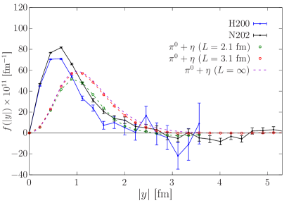
Figure 11: Study of FSEs for Method 2. Left: Integrand for the ensembles H200 and N202 with $m_{\pi}L=4.4$ and $6.4$ respectively. Right: Value of $a_{\mu}^{\rm conn}$ for the ensemble N202 using the FSE correction prescription described in the text, as a function of $|y|_{\rm cut}$.

The left plot of Fig. 11 illustrates the finite-size effect between ensembles N202 and H200, and the discrepancy between these ensembles that differ only by volume is significant. The pion-pole prediction describes the tails of both data-sets reasonably well at large-enough values of $|y|$, although it completely under-estimates the position and height of the short-distance peak of the integrand. It is also worth noting how less statistically precise the result of H200 is compared to N202 for a comparable number of measurements; this gives some indication that the statistical precision is linked to either $m_{\pi}L$ or the physical volume. It is clear that much like for Method 1 there is a significant signal-to-noise problem for large values of $|y|$.

We perform the same finite-size correction procedure for Method 2 as we did for Method 1 above. On the right of Fig. 11 we show the stability of performing the FSE correction with varied $|y|_{\rm cut}$ matching point on ensemble N202. We find excellent stability for many different values of $|y|_{\rm cut}$ and the matching point of $2.6$ fm was chosen in an attempt to minimize the total error.

If we consider the results of Table 6 we see good agreement after finite-size correction between ensembles that only differ by volume (compare U103 with H101, and H200 with N202), which suggests that our finite-size correction procedure is sensible. Unlike for Method 1 we see no reason to exclude these smaller volumes from our final extrapolation. An unusual result in our determination in Method 2 comes from the ensemble N300, which lies below the trend of all our other data points. Since it is the finest ensemble, we have no reason to exclude it, even though this point will reduce the quality of our final extrapolations.

We hold off on presenting the continuum-limit extrapolation here as we will employ a combined extrapolation after the next section (See Sec. VII.1, Fig. 14). However, we will quote the result of the connected continuum extrapolation,

$$a_{\mu}^{\text{conn,M2}}=98.9(2.5)\times 10^{-11}.$$ (22)

The quoted error is a combination of the statistical and 100%-correlated finite-size systematic. We observe that within error this value is in complete agreement with the determination of Method 1.

V.3 Comparison of the two methods

Calculation	$N_{\text{Conf}}$	$N_{\text{Src}}$	$N_{\text{Prop}}$
Method 1	$800$	$48$	$280,800$
Method 2	$901$	$25$	$22,525$
Disconnected	$225$	$480$	$108,000$

Table 7: Resources used for the calculations on ensemble N202. $N_{\text{Conf}}$ gives the number of gauge configurations used, $N_{\text{Src}}$ the number of source positions per gauge configuration, and $N_{\text{Prop}}$ the total number of propagator solves.

The appeal of Method 2 for computing the connected contribution is mostly practical: it is computationally far less expensive than Method 1. The saving between the two is roughly an order of magnitude, see Tab. 7 for a exemplary comparison of computational cost for one particular ensemble, N202. This is because Method 2 effectively replaces sequential propagator solves by additional, much cheaper, QED kernel evaluations. The downside of using these additional kernels is that their combination tends to broaden the integrand $f(|y|)$. This behavior was seen in the lepton loop study of Appendix B and is also clearly the case with all the lattice QCD data in this work. We can use the parameter $\Lambda$ of Eq. (7) to partially ameliorate this broadening; the use of such a subtraction kernel appears to be very important specifically for Method 2, as this regulator offers little to no advantage for Method 1.

If we compare the results for the integrand of H200 and N202 using Method 1 with those of Method 2 (Figs. 8 and 11 respectively) we see that the integrand for Method 2 is in general less-peaked at short distances and extends further in $|y|$. For example, the integrand for N202 using Method 1 is effectively zero around 2 fm, whereas for Method 2 it becomes zero closer to 3 fm. This behavior is reflected in Tables 5 and 6 by larger choices of $|y|_{\text{cut}}$ for Method 2 compared to Method 1.

Again comparing Tables 5 and 6, we see that for both methods the smaller boxes (those with $m_{\pi}L<5$) require a significant finite volume correction. As the data for Method 2 uses the direction $(1,1,1,3)$ we approach the boundary of the lattice ($L/2$) slowly for increasing $|y|$, and so the finite volume effect is smaller in comparison to the direction used in Method 1. We do, however, see somewhat larger discretization effects for Method 2 compared to those found in Method 1, perhaps $O(15\%)$ opposed to $O(10\%)$ at our coarsest lattice spacing respectively. It is quite possible this is due to the $\Lambda$-regulator enhancing the integrand at shorter distances. Nevertheless, this is not a significant problem as we have several fine lattice spacings to help determine the continuum limit.

If we were to use $\Lambda=0.0$ with Method 2 the tail would extend even further into the region where finite-volume effects become significant. This is likely still controllable for the symmetric-point ensembles used here as they have large volumes and $m_{\pi}L$, but this would become much more problematic for lighter-pion-mass ensembles where the signal is expected to degrade quickly at large distances and the integrand is expected to be even broader.

In the following sections, when we combine the results for the connected and disconnected contributions, we will use the results from Method 2 as our connected contribution. This is because they are statistically more precise while still being consistent with those of Method 1.

VI Results for the quark-disconnected contribution

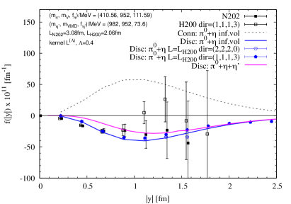
Figure 12: Integrand for the disconnected contribution on ensembles H101 and U103 (left), as well as N202 and H200 (right). The lattice data are shown as black points. The black dashed line shows the fully-connected model prediction, the blue line the $\pi^{0}+\eta$ contribution for the disconnected and the magenta line gives the $\pi^{0}+\eta+\eta^{\prime}$. The blue points show the $\pi^{0}+\eta$ contribution in finite volume.

Table 8 lists the ensembles and statistics used for the computation of the quark-disconnected contribution. As the smaller ensembles (U103, H101, B450, H200) were considerably cheaper to perform inversions on, their statistics is greatly enhanced. As the lattice volume increases, the cost of propagator inversions increases with some power $V^{n}$, with $n>1$, and this quickly becomes the dominant cost of the computation. The column $N_{\text{Src}}$ indicates the number of point-source propagators inverted per gauge configuration to build the grid and the final column indicates the maximum and minimum number of equivalent values of $|y|$ available from the set-up. For the ensembles with open boundary conditions, the number of self-averages, $N_{\rm{Equiv}}$, for a given $|y|$ decreases as $|y|/a$ increases. Therefore open temporal boundaries make this calculation much more difficult as the signal degrades rapidly with large $|y|/a$.

Label	$(t_{\text{min}},t_{\text{max}})/a$	$N_{\text{Src}}$	$N_{\rm Conf}$	$N_{\rm{Equiv}}$(max,min)
U103	$(20,107)$	360	1030	(2112,432)
H101	$(24,72)$	272	1008	(1568,128)
B450∗	$(0,64)$	128	1611	(512,128)
H200	$(24,72)$	272	500	(1568,128)
N202	$(36,93)$	480	225	(2784,672)
N300	$(27,99)$	600	271	(3504,1152)

Table 8: The setup used for each ensemble in the computation of the quark-disconnected contribution. $N_{\text{Src}}$ gives the number of propagator inversions per configuration, $N_{\rm{Conf}}$ gives the number of gauge configurations used and $N_{\rm{Equiv}}$ gives the maximum and minimum number of equivalent values of $|y|$ averaged per configuration. Shorter separations have larger numbers of self-averages, whereas larger values of $|y|$ have smaller $N_{\rm{Equiv}}$. The ensemble B450 has a periodic temporal boundary and temporal length of $2\times$ that of the the spatial, so values of $y/a=n(2,2,2,4)$ could be used, as well as the full periodicity in time.

The ensemble B450 has lattice volume $32^{3}\times 64$ and periodic boundary condition in time, so a fully-periodic grid built of the two basis vectors $(4,4,4,0)$ and $(2,2,2,4)$ was used. All of the other determinations had multiples of $(1,1,1,3)$ and $(2,2,2,0)$ $|y|$ directions, so it is possible that B450 might have noticeably different discretization and finite-volume effects as this direction lies in a different lattice irreducible representation of the broken rotation group $O(4)$. However, as we see in Figs. 12 and 13 the short-distance contribution to the integral is small, and so we can assume the same is true of the discretization effects. As we appropriately correct for FSEs with this choice of direction, we do not expect a significant discrepancy compared to the open-boundary data. Upon continuum extrapolation (Fig. 14) it does seem that this ensemble is consistent with the others, indicating that rotation-breaking artifacts are not the main source of discretization effects.

The integrand for the disconnected contribution is displayed in Fig. 12 for the value $\Lambda=0.4$; much like for Method 2 we find this value to be preferable. The integrand is compared to the prediction for the exchange of the $\pi^{0}$ and $\eta$ mesons with a VMD TFF. In addition, the same prediction including an estimate of the $\eta^{\prime}$ contribution, based on the assumptions in Section IV.3, is indicated.

We do not see any statistically significant finite-volume effects in the integrands between the ensembles U103 and H101, and H200 and N202, for $|y|<1\,$fm. This observation is consistent with the predictions for the $(\pi^{0},\eta)$ exchange in finite volume. The central values of the integrand obtained on ensembles with different volumes differ substantially at some larger values of $|y|$, however this is also in the regime where the signal is rapidly deteriorating, if not lost already. There is a trend in the tail for the larger-volume results to enhance the magnitude of the disconnected contribution, much like what we saw in the connected contribution. We see some enhancement of the integrand compared to the $\pi^{0}+\eta+\eta^{\prime}$ prediction at short distances; the likely cause of this is the contribution from scalar mesons.

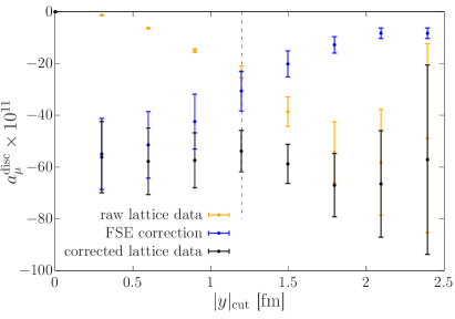
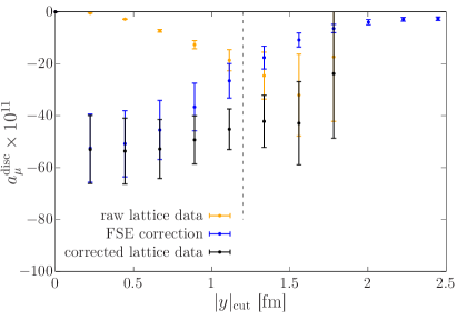
Figure 13: Value of $a_{\mu}^{\rm disc}$ as a function of $|y|_{\rm cut}$ for ensembles H101 (left) and N202 (right).

Clearly, the $\pi^{0}$ and $\eta$ exchanges already provide a rather good description of the shape of the integrand, unlike in the case of the connected contribution (e.g. Figs. 8 and 11). At the same time, the loss of the signal beyond 1.2 fm means that we cannot, at this point, confirm the validity of the $(\pi^{0},\eta)$ exchange at long distances. Given the rapid degradation in signal of the disconnected data, probing large distances of the disconnected contribution will be a very challenging undertaking. There are however good reasons to believe that this description should apply in that regime, and in the following we assume this to be the case.

Label	$a_{\mu}^{\rm data}$	$a_{\mu}^{\rm FSE}$	$a_{\mu}^{\mathrm{tail};\pi^{0}+\eta}$	$a_{\mu}^{\mathrm{tail};\eta^{\prime}}$	$a_{\mu}^{\text{disc}}$
U103	$-17.7(1.9)$	$-2.4$	$-30.0$	4.11	$-45.9(1.9)(7.1)$
H101	$-23.4(2.3)$	$-0.6$	$-30.0$	4.11	$-49.8(2.3)(6.6)$
B450	$-26.7(3.4)$	$-0.9$	$-28.4$	4.11	$-51.8(3.4)(6.3)$
H200	$-12.6(3.7)$	$-2.2$	$-28.2$	4.14	$-38.9(3.7)(6.6)$
N202	$-21.0(6.0)$	$-0.2$	$-28.2$	4.14	$-45.3(6.0)(6.1)$
N300	$-20.6(5.4)$	$-0.7$	$-24.7$	4.01	$-42.0(5.4)(5.4)$

Table 9: Finite-volume corrected disconnected contributions to $a_{\mu}^{\text{hlbl}}$ at the SU$(3)_{\text{\rm f}}$-symmetric point. A breakdown of the FSE contributions to the total results are shown, again a $25\%$ systematic to the total finite-size correction is used. The value of $|y|_{\text{cut}}$ was $1.2\text{ fm}$ for each ensemble.

Table 9 summarizes our results. We perform the FSE matching at a single linearly-interpolated point of $|y|_{\rm cut}=1.2\>\text{fm}$. This point appears to be where we start losing signal for most of our ensembles, and so a significant proportion of the tail of the integrand has to be modelled. We take solace in the fact that the model appears to describe our data well even at distances far shorter than 1.2 fm, as can be seen in Figs. 12 and 13. By far the largest part of the correction comes from modelling the tail with the $(\pi^{0},\eta)$ exchange. This correction is of the order of $100\%$ of the lattice-determined contribution. We have also computed an estimate of the $\eta^{\prime}$ exchange contribution as described in section IV.3. The values in Table 9 show that its contribution to the tail, $|y|>1.2$ fm, is much smaller. Its magnitude is covered by the systematic uncertainty we assign to the modelling of the tail. We have chosen to include the estimated contribution of the $\eta^{\prime}$ to the tail in the central value of $a_{\mu}^{\rm disc}$.

Anticipating the combined analysis presented in section VII.1, the continuum-extrapolated disconnected value we obtain from a constrained-slope fit to both the connected Method 2 data and the disconnected data is

$$a_{\mu}^{\rm disc}=-33.5(4.2)\times 10^{-11}.$$ (23)

We observe that this result amounts to be about $(-1/3)$ of the connected contribution.

VII The total $a_{\mu}^{\rm hlbl}$

The main purpose of this section is to describe how we arrive at our final result for the total $a_{\mu}^{\rm hlbl}$ (subsection VII.1), in which the systematics of the continuum extrapolation are discussed in detail. The following sub-section VII.2 presents a study of the dependence of our result on the muon mass, and finally, subsection VII.3 discusses what outcome one may expect for $a_{\mu}^{\rm hlbl}$ at physical quark masses based on our findings.

VII.1 Final result for $a_{\mu}^{\rm hlbl}$ in SU$(3)_{\rm f}$-symmetric QCD

VII.1.1 Combining the connected and disconnected contributions

In order to obtain the final result for $a_{\mu}^{\rm hlbl}=a_{\mu}^{\rm conn}+a_{\mu}^{\rm disc}$, we combine the disconnected data with the connected data of Method 2, as it is consistent with, yet statistically more precise than that of Method 1. We then perform two analyses on this combined data set. The full set of data for the two contributions and their sum is shown in Fig. 14, along with fits and results from the first analysis whose description follows. Both the connected and disconnected data show a negative slope in $a^{2}$ despite the two contributions having opposite signs. This indicates that the leading discretization effects do not arise from a common multiplicative effect such as the renormalization factor.

The first analysis consists in simultaneously extrapolating both the connected and the disconnected contributions to the continuum with a slope in $a^{2}$ constrained to be equal for the two contributions, before summing the two constant parameters of the fit to obtain $a_{\mu}^{\rm hlbl}$. In this procedure, the results for the connected contribution and the disconnected contribution are both corrected for finite-size effects and for the extension of the $|y|$-integrand. The statistical errors are obtained under the bootstrap, and a correlated gaussian sample with appropriate width is propagated for the systematic error due to the correction. The systematic error of the correction, which is set to $25\%$ of its size, is treated as being fully anti-correlated between the connected and the disconnected contribution (recall that the two contributions have opposite sign). The fit ansatz for the two continuum extrapolations is a polynomial of degree one in $a^{2}$. For this analysis we obtain the result,

$$a_{\mu}^{\rm hlbl}=65.4(4.9)\times 10^{-11}.$$ (24)

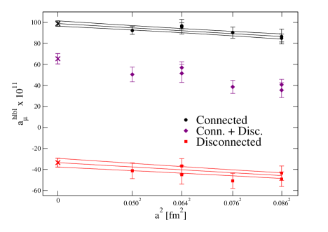
Figure 14: Combined continuum-extrapolation analysis for the connected and disconnected data. The fits were constrained to have the same slope and the final sum of the two was performed on the constant fit parameters. Also shown is the individual sum of the connected and disconnected pieces. The purple cross represents the addition of the continuum-extrapolated results for the connected and disconnected contributions.

In the second analysis method, the connected and disconnected contributions are summed prior to performing the continuum extrapolation. This extrapolation is then performed linearly in $a^{2}$. In this analysis, the correction applied to the lattice data is split into two parts, (a) $a_{\mu}^{\rm FSE}$, the pure finite-size correction on the integrand, and (b) $a_{\mu}^{\rm tail}$, the extension of the integrand beyond some $|y|_{\rm cut}$. In combining the connected and disconnected contributions, each part is treated as being fully anti-correlated between the connected and the disconnected contribution; however, in contrast with the first analysis, the correlation between the systematic errors of the two parts is considered to be zero. The alternative point of view adopted here is that predicting the tail of the infinite-volume integrand is a rather different exercise from predicting the finite-size effect on the finite-volume integrand; one of the two predictions could be successful while the other is not. The result of this procedure is

$$a_{\mu}^{\rm hlbl}=64.5(6.7)\times 10^{-11}.$$ (25)

The two analyses produce compatible values for $a_{\mu}^{\rm hlbl}$ but the first is more precise and allows more flexibility since the two contributions are treated separately. Therefore, we will use the first analysis for the final result and study variations on it to estimate the systematic uncertainty.

VII.1.2 Continuum extrapolation systematics

Our data are noisy and it is difficult to find a fit that describes them perfectly, so we identify several different choices of continuum extrapolation to investigate the spread and provide an associated continuum-extrapolation systematic. We note that (also expressed in Sec. V.1) as we are not using the $O(a)$-improved vector currents it is possible that we have a term linear in the lattice spacing. We consider the two fit forms:

$$a_{\mu}^{\text{conn}}(a)=a_{\mu}^{\text{conn}}(0)+Aa^{n},\qquad a_{\mu}^{\text{disc}}(a)=a_{\mu}^{\text{disc}}(0)+Ba^{m},$$ (26)

with various cuts to the data, constraints on $A$ and $B$, and choices of $n$ and $m$ as listed in Table 10. We then add the distributions $a_{\mu}^{\rm hlbl}=a_{\mu}^{\text{conn}}(0)+a_{\mu}^{\text{disc}}(0)$ to obtain the results shown in Fig. 15.

Index	$a$-Cut [fm]	Constraint	$n$	$m$	Index	$a$-Cut [fm]	Constraint	$n$	$m$
1	None	None	1	1	6	None	None	2	2
2	None	$A=B$	1	1	7	None	$A=B$	2	2
3	None	$B=0$	1	-	8	None	$B=0$	2	-
4	$<0.0864$	None	1	1	9	$<0.0864$	None	2	2
5	$<0.0864$	$A=B$	1	1	10	$<0.0864$	$A=B$	2	2

Table 10: Different fit forms used to estimate the continuum extrapolation systematic.

It is clear that any time we omit the coarse data the fit wants to flatten the slope. This is due to the anomalously low result of N300. When we do not include the coarse ensembles the error increases substantially, which is fairly indicative that the fit is struggling to accurately model the data.

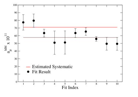
Figure 15: An estimate of our continuum extrapolation systematic on the full $a_{\mu}^{\rm hlbl}$ for the combination of Method 2 and the disconnected data.

If we perform a fit linear in $a$ the central value moves up, as was also the case for the Method 1 continuum extrapolation. We choose to quote the linear in $a^{2}$ fit to all the data with a constrained slope as our final result as it has the best $\chi^{2}/\mathrm{d.o.f.}=2$. For the continuum-extrapolation systematic, we use the lower error bound of the largest fit result and the upper bound of our lowest fit result. It is clear that constraining the slope or letting it vary does little to the position of the central value apart from reducing the error, this suggests that the fit is having a hard time accurately determining the slope with the quality of the data we have at present.

VII.2 The dependence of our results on the muon mass

Since the mesons at the SU(3)_f-symmetric point can be viewed as ‘heavy’ degrees of freedom relative to the muon, we would expect $a_{\mu}^{\rm hlbl}$ to be roughly proportional to $m_{\mu}^{2}$. Here, we will study what happens if we re-scale the muon mass on one of our ensembles. We are motivated to do so by our experience on related projects Gérardin et al. (2019c) whereby adjusting the muon mass by some dimensionless ratio can flatten the approach to the chiral limit. Here we investigate this idea by defining two quantities,

$$\overline{a}^{\text{hlbl}}_{\mu}=\left(\frac{f_{\pi}^{\text{Latt.}}}{f_{\pi}^{\text{Phys.}}}\right)^{2}a_{\mu}^{\rm hlbl}(m_{\mu}^{\text{Phys.}}),$$ (27)

and,

$$\quad\tilde{a}^{\text{hlbl}}_{\mu}=a_{\mu}^{\text{hlbl}}\left(\frac{f_{\pi}^{\text{Latt.}}}{f_{\pi}^{\text{Phys.}}}m_{\mu}^{\text{Phys.}}\right).$$ (28)

The first quantity rescales the integrated result by the lattice-determined pion decay constant divided by the value in continuum, squared. The second quantity re-scales the muon mass used as input in our determination by this ratio. These two definitions would be comparable if $a_{\mu}^{\rm hlbl}$ scales as $m_{\mu}^{2}$, which is to be expected in the heavy-quark limit.

Fig. 16 illustrates the effect of these re-scaling procedures on the connected contribution to $a_{\mu}^{\rm hlbl}$ on one of our coarsest and largest boxes, H101 (results are from Method 2 with $\Lambda=0.4$). It is clear that these two prescriptions are equivalent within error, which suggests that any change in the muon mass leads to a quadratic change in the integrated result. We can also use this analysis to very naively infer how much we expect the result to grow as we approach the chiral limit, and it appears that for the connected contribution this could be of the order of a $25\%$ increase.

Figure 16: Partially-integrated lattice results for the ensemble H101 with and without re-scaling of the integral.

VII.3 Expectations for $a_{\mu}^{\rm hlbl}$ in QCD with physical quark masses

In this subsection, we first quantify the contributions to $a_{\mu}^{\rm hlbl}$ at the SU$(3)_{\rm f}$-symmetric point not coming from the light pseudoscalars. These contributions are expected to have only a modest quark-mass dependence, and they are also the hardest to determine quantitatively by (experimental-)data-driven methods. Therefore any information on these contributions is worthwhile collecting. By using our determination of this contribution together with our previous calculation of the $\pi^{0}$ exchange, we can arrive at an estimate for $a_{\mu}^{\rm hlbl}$ at physical quark masses.

We begin by noting that, subtracting the $\pi^{0}$ and $\eta$ contributions (respectively Eqs. (16) and (18)) from our final SU(3)-point result (31), the contribution of heavier intermediate states amounts to

$$a_{\mu}^{\rm hlbl,SU(3)_{\rm f}}-a_{\mu}^{\rm hlbl,\pi^{0}+\eta,SU(3)_{\rm f}}=(37.4\pm 8.3)\times 10^{-11}.$$ (29)

In particular, this contribution accounts for 57% of the total $a_{\mu}^{\rm hlbl}$, and we have added all statistical and systematic errors in quadrature.

Next, we may try to roughly estimate $a_{\mu}^{\rm hlbl}$ at the physical point. As the $(u,d)$ quark masses are lowered to their physical values at fixed trace of the quark mass matrix, it is the pion whose mass changes by the largest factor: it becomes a factor of three lighter. Since we have an evaluation of the $\pi^{0}$ exchange contribution at the SU$(3)_{\rm f}$-symmetric point and at the physical point (see Eqs. (16–17)), we can correct for this effect,

$$a_{\mu}^{\rm hlbl,SU(3)_{\rm f}}-a_{\mu}^{\rm hlbl,\pi^{0},SU(3)_{\rm f}}+a_{\mu}^{\rm hlbl,\pi^{0},{\rm phys}}=(104.1\pm 9.1)\times 10^{-11}.$$ (30)

One can think of Eq. (30) as a rough estimate of $a_{\mu}^{\rm hlbl}$ at the physical point, purely based on our lattice QCD results and the assumption of a negligible quark-mass dependence of the non-$\pi^{0}$-exchange contributions. As argued in the next paragraph, we expect such an estimate to hold at the 20% level. It is well in line with the most recent evaluations Aoyama et al. (2020).

In order to assess the systematic uncertainty of such an estimate, we perform a slightly more sophisticated method to correct for the quark-mass dependence of the $\eta$ contribution and the charged pion loop. Within the scalar QED framework, we find $-6.3\times 10^{-11}$ for the pion loop, to be doubled to include the kaon loop, and we expect a factor of two to three reduction if one includes an electromagnetic form factor for the pseudoscalar. Therefore, further subtracting $a_{\mu}^{{\rm hlbl},(\pi^{\pm},K^{\pm}),{\rm SU}(3)_{\rm f}}\approx 2\times(-3.0)\times 10^{-11}$ from Eq. (29), we obtain $(43.4\pm 9.3)\times 10^{-11}$. This number represents our estimate of the non-pseudo-Goldstone contributions at the SU$(3)_{\rm f}$ -symmetric point. We observe that by neglecting the quark-mass dependence of this contribution, and using the dispersive $\pi^{0}$-exchange Hoferichter et al. (2018); Aoyama et al. (2020) and the Canberbury-approximant $\eta$-exchange Masjuan and Sanchez-Puertas (2017); Aoyama et al. (2020) results for $a_{\mu}^{\rm hlbl,\pi^{0}+\eta,{\rm phys}}=79.3\times 10^{-11}$ and the box contribution Colangelo et al. (2017); Aoyama et al. (2020) to $a_{\mu}^{{\rm hlbl},(\pi^{\pm},K^{\pm}),{\rm phys}}=-16.4\times 10^{-11}$, we arrive at the estimate $10^{11}a_{\mu}^{\rm hlbl,phys}=79.3(3.0)-16.4(2)+43.4(9.3)=106.3(9.8)$. It is only slightly different from the more naive estimate of Eq. (30). Therefore we consider it safe to assign a systematic error of 20% to Eq. (30) as an estimate of $a_{\mu}^{\rm hlbl}$ at the physical point. This uncertainty estimate also generously covers the $a_{\mu}^{\rm hlbl,phys}$ value obtained by assuming that the non-pseudo-Goldstone contributions increase from the SU(3)_f to the physical point by a factor $(f_{\pi}^{\rm SU(3)_{\rm f}}/f_{\pi}^{\rm phys})^{2}$ to account approximately for the quark-mass dependence of the QCD resonances; see the previous subsection concerning this point.

VIII Conclusions

In this work we have computed the hadronic light-by-light contribution to the $g-2$ of the muon using lattice QCD at the SU$(3)_{\text{\rm f}}$-symmetric point with $m_{\pi}=m_{K}\approx 420$ MeV. We chose to initially work at the symmetric point for several reasons: Due to the significantly reduced computational cost (as compared to simulations at physical quark masses), we are able to control all known sources of systematic error, in particular the finite-size and finite lattice spacing effects. Second, the SU(3)_f-symmetry implies that only two out of five quark-contraction topologies contribute, and it simplifies the hadronic models with which the integrand can be compared and interpreted. For instance, the $\eta$-exchange contribution simply amounts to one third of the pion-exchange. Third, the overall contribution from states beyond the light pseudoscalars is not expected to be strongly quark-mass dependent, so that the present calculation already constrains its size.

In order to help interpret our results for $a_{\mu}^{\rm hlbl}$, we have performed an exploratory study of the low-lying meson spectrum at the SU(3)_f point. The most remarkable feature is the existence of a stable singlet $J^{PC}=0^{++}$ meson with a mass of about 680 MeV. Also, our previous calculation of the pion transition form factor Gérardin et al. (2019a) allows us to quantify the contributions of the $\pi^{0}$ and $\eta$ exchanges.

Our strategy to calculate $a_{\mu}^{\rm hlbl}$ relies on coordinate-space perturbation theory, for which muon and photon propagators are computed in infinite volume. We have presented the integrand for the final, one-dimensional integral over the distance $|y|$ of a quark-photon vertex from one of the other two internal vertices, since it contains more information than the final $a_{\mu}^{\rm hlbl}$ value. For the quark-connected contribution we have identified two methods of calculation that we call Method 1 and Method 2. The former amounts to a direct computation of the three connected diagrams, but it is a numerically costly approach, as it involves many sequential-propagator calculations. To make this computation much cheaper, we have utilized several changes of variables and translational invariance to rewrite the integral in terms of an easy-to-calculate single diagram and a combination of different kernels; this we call Method 2.

For a single $|y|$-value, Method 2 requires only two propagator inversions, at the meagre cost of a more-complicated QED-kernel calculation. Method 2 has another computational advantage over Method 1 in that it allows one to store a set of propagators in memory and perform their integrals, redefining the origin to be each propagator source; thereby, for $N$ propagators we can compute $N(N-1)$ non-zero samples of $f(|y|)$. If the source points are evenly spaced and the volume is periodic this amounts to $N$ self-averages per $|y|$. Such self-averaging is crucial in reducing the cost of the calculation.

We note that the combination of kernels needed for Method 2 broadens the integrand in $|y|$ significantly. To counteract this effect, we have introduced a new class of subtracted kernels with a gaussian-regulator $\Lambda$. This parameter $\Lambda$ effectively allows us to tune the shape of the integrand to peak at shorter-distances. We find that a value of $\Lambda=0.4$ suits our purposes quite well and allows for the integral of the connected lattice data to saturate at reasonably short distances of about $2\text{ fm}$.

We have handled the disconnected contribution by introducing a sparse sub-grid of equi-distant point sources, the idea being that we obtain a large number of self-averages from treating our origin as each point on the grid. Such a technique is necessary as this contribution is extremely noisy and suffers from a significant signal-to-noise problem at large distances. We note that potentially millions of averages are needed in order to get good control over errors at distances of order $2\text{ fm}$.

In our calculation, we have seen that finite-size effects are significant, and having a good theoretical understanding of the tail of the integrand is very important. For the quark-connected contribution, we have approximated the $\pi^{0}$ and $\eta$ meson exchange contribution to the integrand using a vector-dominance transition form factor and compared it to the lattice data; only at fairly large $|y|$ does the prediction quantitatively represent the integrand. We therefore attempt to conservatively incorporate as much lattice data as possible before making contact with the model. For the disconnected contribution, the model does a satisfactory job of describing the data over the entire range of $|y|$ where we have signal, and we therefore match on to the prediction at shorter distances, where we still have control over the statistical errors of the lattice data.

We have shown that both the disconnected and connected contributions have a non-negligible discretization effect within our measured precision. It appears to be of the same sign and comparable magnitude for both contributions, but ultimately this extrapolation appears well under control. We decide to quote a result from a fit linear in $a^{2}$ with a constrained slope to the data of Method 2 and the disconnected as,

$$a_{\mu}^{\rm hlbl}=(65.4\pm 4.9\pm 6.6)\times 10^{-11},$$ (31)

at the SU(3) flavor-symmetric point, where the first error results from the uncertainties on the individual gauge ensembles, and the second is the systematic error of the continuum extrapolation.

We have discussed in subsection VII.3 how we expect our result for $a_{\mu}^{\rm hlbl}$ to evolve as the up and down quark masses are lowered towards their physical values at fixed trace of the quark mass matrix. Correcting for the increase in the $\pi^{0}$ exchange contribution using our previous lattice calculation Gérardin et al. (2019a), we arrive at a value (Eq. (30)) which is very well in line with the most recent phenomenological Aoyama et al. (2020) and lattice QCD results Blum et al. (2020). This value is quite stable under varying the assumptions about the quark-mass dependence of heavier-state contributions.

In order to reduce the systematic uncertainty of $a_{\mu}^{\rm hlbl}$ at physical quark masses using lattice QCD, obviously simulations at lighter quark masses are needed. The methods we have developed to correct for finite-size effects and to extend the tail of the $|y|$-integrand based on the $\pi^{0}$ exchange will be extremely valuable in this endeavor. While we have reached a semi-quantitative understanding of the integrand in terms of hadronic models, further work is needed on the theory side to bring this description to a fully quantitative level.

Appendix A Pseudoscalar-meson-exchange-channel matching in Method 2 and the quark-disconnected contribution

In this work, when we compute the quark-connected diagrams using Method 2 and the quark-disconnected diagrams, only a subset of Feynman diagrams are considered due to the contributing Wick-contractions at QCD level. In order to study the FSE in an effective field theory framework, one has to map these contractions to the corresponding Feynman diagrams in the effective theory. Our study of the FSE is based on pseudoscalar-meson (PS) exchange from Chiral Perturbation Theory. The matching between the QCD Feynman diagrams and the PS-meson-exchange channels can be done in various ways. Here, we present a determination of the matching using Partially-Quenched QCD (PQQCD) and Partially-Quenched Chiral Perturbation Theory (PQChPT). There have been many applications of PQQCD in the Lattice QCD community (see e.g. Bernard and Golterman (1992); Sharpe and Shoresh (2000); Giusti and Lüscher (2009)). In particular, it can serve as a tool to give an estimate of the size of the contribution coming from quark-disconnected diagrams compared to the connected ones for some observables Della Morte and Jüttner (2010). Here we do not intend to detail the formalism, but only to give some arguments to explain how we reach the mappings explained in our methodology.

PQQCD is a theory with a graded Lie-group SU$(N|M)$ as symmetry group. In this theory there are $N-M$ sea quarks and $M$ valence (quenched) quarks with their ghost counterparts. The presence of these quenched quarks does not change the partition function from the un-quenched theory with $N-M$ dynamical quarks. Therefore, one can formulate each of the different Wick contractions needed for computing an $n$-point function (in an un-quenched theory) in a partially-quenched theory by adding certain number of quenched quarks. Then, one can study the long-distance behavior of the observable using PQChPT, which is the corresponding effective field theory to PQQCD.

With only three flavors (as is the case in this work), one cannot build a four-point function that requires only quark-connected diagrams, because each quark line would require a different flavor in order to avoid disconnected diagrams. However, such a four-point function can be constructed with an additional quenched quark flavor, i.e. SU$(4|1)$ PQQCD. For instance, if we introduce a quenched quark $r$ and its ghost $\tilde{r}$ with the same mass as the ones originally present in the SU$(3)_{\rm f}$ theory, namely $u$, $d$ and $s$, in the computation of the four-point function

$$\langle\bar{u}\gamma_{\mu}d(x)\bar{d}\gamma_{\nu}s(y)\bar{s}\gamma_{\sigma}r(z)\bar{r}\gamma_{\sigma}u(0)+h.c.\rangle,$$ (32)

only quark-connected diagrams are involved. Eq. (32) is exactly the four-point function $\widetilde{\Pi}^{(1)}_{\mu\nu\sigma\lambda}(x,y,z,0)$ that is used for the connected contribution in Method 2.

Moreover, one can study the quark-disconnected diagrams that we consider in this work within the same partially quenched theory. For instance,

$$\langle\bar{u}\gamma_{\mu}d(x)\bar{d}\gamma_{\nu}u(y)\bar{s}\gamma_{\sigma}r(z)\bar{r}\gamma_{\sigma}s(0)+h.c.\rangle$$ (33)

only contains the disconnected diagram where $(x,y)$ and $(z,0)$ are connected by quark lines.

To determine the relevent PS-meson-exchange channel, one can consider the Wess-Zumino-Witten term Wess and Zumino (1971); Witten (1983) in PQChPT at leading order in the decay constant. Eq. (32) can be understood as a four-point vector current correlation function. A general procedure is to include all the possible super traces of operators Detmold et al. (2006). However, in the case of the coupling to external charged vector currents, which are the Noether currents of the symmetry group SU$(N|M)$ whose generators are super-traceless, the only allowed non-vanishing term is proportional to

$$\textrm{str}(T^{a}T^{b}T^{c})\int d^{4}x\phi^{c}\epsilon^{\mu\nu\rho\sigma}F^{a}_{\mu\nu}F^{b}_{\rho\sigma},$$ (34)

where $\phi$ is the Goldstone boson/ghost field, $F_{\mu\nu}$ is the field strength of the external vector current and the $T^{a}$’s are the generators of the group. As a result, in momentum-space, the PS-meson exchange in the $s$-channel of the two-vector-currents-to-two-vector-currents process $v^{a_{1}}v^{b_{1}}\rightarrow v^{a_{2}}v^{b_{2}}$ is proportional to

$$\textrm{str}(\{T^{a_{1}},T^{b_{1}}\}T^{c_{1}})\textrm{str}(\{T^{a_{2}},T^{b_{2}}\}T^{c_{2}})g^{c_{1}c_{2}}G(p^{2}),$$ (35)

where $G$ is the scalar field propagator ,

$$G(p^{2})=\frac{1}{p^{2}+m_{\pi}^{2}},$$ (36)

and

$$g^{ab}=2\textrm{str}(T^{a}T^{b}).$$ (37)

The matching between different contractions and the PS-exchange channels based on this computation is shown in Fig. 17.

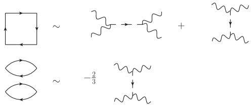
Figure 17: Correspondence between connected (Method 2) and disconnected diagrams (left) and PS-meson exchange channels (right) in position space of the four-point functions described in the text. The top-left figure should be understood as containing quark flow in both orientations, representing exactly all the relevent diagrams for Method 2. Note that the charge factors are not included here.

With the charge factors included, one will recover the ratio between the total quark-disconnected contribution and the total quark-connected given in Ref. Gérardin et al. (2018), based on charge factor arguments.

Appendix B The new subtraction with the lepton-loop

In this section we investigate the new subtraction for both Methods 1 and 2 using the infinite volume lepton-loop. A comparison of previous results with our kernel to the lepton-loop can be found in Asmussen et al. (2018, 2020). The lepton-loop result can be determined easily by standard numerical integration techniques, the results of which can be used to inform our choices of kernel parameters in the full QCD calculation.

For both figures (18 and 19) we set the lepton mass equal to that of the muon.

Fig. 18 shows the results for Method 1. There is little difference between the choices of $\Lambda$ for this calculation and they all saturate the integral reasonably quickly. The result when $\Lambda=\infty$ is too peaked at short distances to make this a useful kernel for the lattice computation. All of the peak positions for the integrands are roughly at the same (small) value of $|y|$.

In Fig. 19 we show the results for Method 2. We see that the usual kernel ($\Lambda=\infty$) is very peaked at short distances, this will make it unsuitable for the lattice calculation. We also note that $\Lambda=0$ gives a broad integrand that very slowly approaches the exact result, this also makes it somewhat unsuitable for a lattice calculation unless a large physical volume and large values of $|y|$ are available.

The choice of $\Lambda=0.4$ has a slightly more pronounced peak at small $|y|$ than $\Lambda=0$ and it goes to zero at large distances rapidly. There is a small negative contribution to the integral at large $|y|$, but in the full QCD case can be corrected for by modelling the tail, as $\Lambda$ increases this negative correction grows. If our lepton-loop result translates to full QCD this choice of $\Lambda$ should allow for most of our integral to be encompassed by the lattice volume.

(a) Method 1 integrands

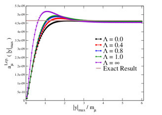
(b) Method 1 integrals

Figure 18: Left: the integrands in Method 1 of several $\Lambda$ choices of the new subtracted kernel. Right: the results of the partial integration of the integrands up to some $|y|_{\text{max}}$. These results were obtained with lepton mass equal to the muon mass and the exact result used was $4.6497\times 10^{-9}$ Laporta and Remiddi (1993).

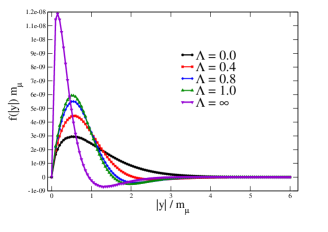
(a) Method 2 integrands

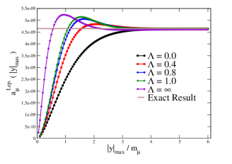
(b) Method 2 integrals

Figure 19: Same as Fig. 18 but for Method 2.

If we compare the two methods using the lepton-loop we see that the parameter $\Lambda$ makes a significant difference to the integrand for Method 2. Any of the choices $\Lambda=0.0,0.4,0.8,1.0$ seem usable for Method 1. It is interesting to note that Method 2 actively shifts the peak of the integrand to typically intermediate distances. So, with a careful choice of the parameter $\Lambda$ we can tune the kernel to peak in a region where the calculation is not so sensitive to either of the lattice cut-offs of lattice spacing and volume.

Appendix C Kernel independence of $a_{\mu}^{\rm conn}$ and $a_{\mu}^{\rm disc}$

The validity of the subtractions applied to the QED kernel originates from the Ward identity (current conservation) satisfied by the electromagnetic current. Thus, one will expect a kernel-independent result at the level of the total result of $a_{\mu}^{\rm hlbl}$. In this paper, we have treated the contribution from the connected diagrams ($a_{\mu}^{\rm conn}$) and the contribution from the disconnected diagrams ($a_{\mu}^{\rm disc)}$) separately. One natural question would be whether these two quantities themselves are also kernel-independent. The answer to this question is yes, due to the Ward identity satisfied by the vector current. We will give a proof of this statement in the SU$(3)_{f}$ case.
In Euclidean space-time, if an infinitesimal transformation $\delta_{\epsilon}$ of the fields does not change the path integral measure, we have

$${}\langle\delta_{\epsilon}S\mathcal{O}\rangle=\langle\delta_{\epsilon}\mathcal{O}\rangle,$$ (38)

where $S$ is the QCD action and $\mathcal{O}$ is any operator. Without changing the action, we can consider a partially-quenched theory by introducing a quenched quark $r$ and its ghost partner $\tilde{r}$ (see Appendix A). If we consider an infinitesimal transformation generated by the local SU$(2)_{f}$ symmetry of the quark pair $(u,d)$ and their conjugates :

$$\begin{split}&\delta_{\epsilon}u(x_{0})=i\epsilon(x_{0})d(x_{0}),\quad\delta_{\epsilon}d(x_{0})=i\epsilon(x_{0})u(x_{0}),\\ &\delta_{\epsilon}\bar{u}(x_{0})=-i\epsilon(x_{0})\bar{d}(x_{0}),\quad\delta_{\epsilon}\bar{d}(x_{0})=-i\epsilon(x_{0})\bar{u}(x_{0}),\end{split}$$ (39)

we have the following expression for the variation of the action related to the corresponding Noether current

$$\delta_{\epsilon}S=i\epsilon(x_{0})\partial_{\lambda}(\bar{u}\gamma_{\lambda}d+\bar{d}\gamma_{\lambda}u)(x_{0}).$$ (40)

We now consider the trilocal operator $\mathcal{O}_{\mu\nu\sigma}(x,y,z):=\bar{u}\gamma_{\mu}d(x)\bar{s}\gamma_{\nu}r(y)\bar{r}\gamma_{\sigma}s(z)$, which transforms as

$$\delta_{\epsilon}\mathcal{O}_{\mu\nu\sigma}(x)=i\epsilon(\bar{u}\gamma_{\mu}u-\bar{d}\gamma_{\mu}d)(x)\bar{s}\gamma_{\nu}r(y)\bar{r}\gamma_{\lambda}s(z).$$ (41)

Plugging in everything in Eq. (38), we have

$$\partial_{\lambda}\langle\bar{u}\gamma_{\mu}d(x)\bar{d}\gamma_{\lambda}u(x_{0})\bar{s}\gamma_{\nu}r(y)\bar{r}\gamma_{\sigma}s(z)\rangle=\partial_{\lambda}\langle\Pi_{\mu\lambda}(x,x_{0})\Pi_{\nu\sigma}(y,z)\rangle_{U}=0,$$ (42)

where $\Pi_{\mu\nu}(x,x_{0})\Pi_{\nu\sigma}(y,z)$ gives one of the contractions needed for the disconnected computation. One can then easily show that all the disconnected diagrams have similar current-conservation property. Consequently, the subtractions that we apply to the QED-kernel do not change the result on the contribution from the disconnected diagrams. It follows directly that the connected contribution is also kernel-independent, because $a_{\mu}^{\rm conn}=a_{\mu}^{\rm hlbl}-a_{\mu}^{\rm disc}$ in our SU$(3)_{f}$ case. One can further show that $a_{\mu}^{\rm conn}$ is also itself kernel-independent in general flavor cases.

References

- Bennett et al. (2006) G. W. Bennett et al. (Muon ), “Final report of the E821 muon anomalous magnetic moment measurement at BNL,” Phys. Rev. D 73, 072003 (2006), arXiv:hep-ex/0602035 .
- Jegerlehner and Nyffeler (2009) F. Jegerlehner and A. Nyffeler, “The muon ,” Phys. Rept. 477, 1 (2009), arXiv:0902.3360 [hep-ph] .
- Blum et al. (2013) T. Blum, A. Denig, I. Logashenko, E. de Rafael, B. Lee Roberts, et al., “The muon theory value: Present and future,” (2013), arXiv:1311.2198 [hep-ph] .
- Jegerlehner (2017) F. Jegerlehner, The Anomalous Magnetic Moment of the Muon (Springer Tracts Mod. Phys., vol. 274, 2017).
- Aoyama et al. (2020) T. Aoyama et al., “The anomalous magnetic moment of the muon in the Standard Model,” (2020), arXiv:2006.04822 [hep-ph] .
- Grange et al. (2015) J. Grange et al. (E989), “Muon technical design report,” (2015), arXiv:1501.06858 [physics.ins-det] .
- Mibe (2011) T. Mibe (J-PARC ), “Measurement of muon and EDM with an ultra-cold muon beam at J-PARC,” Tau lepton physics. Proceedings, 11th International Workshop, TAU 2010, Manchester, UK, September 13-17, 2010, Nucl. Phys. B (Proc. Suppl.) 218, 242 (2011).
- Meyer and Wittig (2019) H. B. Meyer and H. Wittig, “Lattice QCD and the anomalous magnetic moment of the muon,” Prog. Part. Nucl. Phys. 104, 46 (2019), arXiv:1807.09370 [hep-lat] .
- Blum et al. (2017) T. Blum, N. Christ, M. Hayakawa, T. Izubuchi, L. Jin, C. Jung, and C. Lehner, “Connected and leading disconnected hadronic light-by-light contribution to the muon anomalous magnetic moment with a physical pion mass,” Phys. Rev. Lett. 118, 022005 (2017), arXiv:1610.04603 [hep-lat] .
- Asmussen et al. (2019a) N. Asmussen, A. Gérardin, A. Nyffeler, and H. B. Meyer, “Hadronic light-by-light scattering in the anomalous magnetic moment of the muon,” SciPost Phys. Proc. 1, 031 (2019a), arXiv:1811.08320 [hep-lat] .
- Colangelo et al. (2018) G. Colangelo, M. Hoferichter, M. Procura, and P. Stoffer, “Hadronic light-by-light contribution to : a dispersive approach,” Proceedings, 35th International Symposium on Lattice Field Theory (Lattice 2017): Granada, Spain, June 18-24, 2017, EPJ Web Conf. 175, 01025 (2018), arXiv:1711.00281 [hep-ph] .
- Gérardin et al. (2019a) A. Gérardin, H. B. Meyer, and A. Nyffeler, “Lattice calculation of the pion transition form factor with Wilson quarks,” Phys. Rev. D 100, 034520 (2019a), arXiv:1903.09471 [hep-lat] .
- Gronberg et al. (1998) J. Gronberg et al. (CLEO), “Measurements of the meson-photon transition form factors of light pseudoscalar mesons at large momentum transfer,” Phys. Rev. D 57, 33 (1998), arXiv:hep-ex/9707031 .
- del Amo Sanchez et al. (2011) P. del Amo Sanchez et al. (BaBar), “Measurement of the and transition form factors,” Phys. Rev. D 84, 052001 (2011), arXiv:1101.1142 [hep-ex] .
- Lees et al. (2018) J. P. Lees et al. (BaBar), “Measurement of the transition form factor,” Phys. Rev. D 98, 112002 (2018), arXiv:1808.08038 [hep-ex] .
- Blum et al. (2020) T. Blum, N. Christ, M. Hayakawa, T. Izubuchi, L. Jin, C. Jung, and C. Lehner, “Hadronic light-by-light scattering contribution to the muon anomalous magnetic moment from lattice QCD,” Phys. Rev. Lett. 124, 132002 (2020), arXiv:1911.08123 [hep-lat] .
- Asmussen et al. (2020) N. Asmussen, A. Gérardin, J. R. Green, H. B. Meyer, and A. Nyffeler, “Hadronic light-by-light scattering contribution to the muon from lattice QCD: semi-analytical calculation of the QED kernel,” (2020), in preparation.
- Asmussen et al. (2019b) N. Asmussen, E.-H. Chao, A. Gérardin, J. R. Green, R. J. Hudspith, H. B. Meyer, and A. Nyffeler, “Developments in the position-space approach to the HLbL contribution to the muon on the lattice,” Proceedings, 37th International Symposium on Lattice Field Theory (Lattice 2019), Wuhan, China, 16–22 June 2019, (2019b), arXiv:1911.05573 [hep-lat] .
- Gérardin et al. (2019b) A. Gérardin, T. Harris, and H. B. Meyer, “Nonperturbative renormalization and -improvement of the nonsinglet vector current with Wilson fermions and tree-level Symanzik improved gauge action,” Phys. Rev. D 99, 014519 (2019b), arXiv:1811.08209 [hep-lat] .
- Bruno et al. (2015) M. Bruno et al., “Simulation of QCD with flavors of non-perturbatively improved Wilson fermions,” JHEP 02, 043 (2015), arXiv:1411.3982 [hep-lat] .
- Bruno et al. (2017) M. Bruno, T. Korzec, and S. Schaefer, “Setting the scale for the CLS flavor ensembles,” Phys. Rev. D 95, 074504 (2017), arXiv:1608.08900 [hep-lat] .
- Peardon et al. (2009) M. Peardon, J. Bulava, J. Foley, C. Morningstar, J. Dudek, R. G. Edwards, B. Joó, H.-W. Lin, D. G. Richards, and K. J. Juge (Hadron Spectrum), “Novel quark-field creation operator construction for hadronic physics in lattice QCD,” Phys. Rev. D 80, 054506 (2009), arXiv:0905.2160 [hep-lat] .
- Morningstar et al. (2011) C. Morningstar, J. Bulava, J. Foley, K. J. Juge, D. Lenkner, M. Peardon, and C. H. Wong, “Improved stochastic estimation of quark propagation with Laplacian Heaviside smearing in lattice QCD,” Phys. Rev. D 83, 114505 (2011), arXiv:1104.3870 [hep-lat] .
- Briceno et al. (2017) R. A. Briceno, J. J. Dudek, R. G. Edwards, and D. J. Wilson, “Isoscalar scattering and the meson resonance from QCD,” Phys. Rev. Lett. 118, 022002 (2017), arXiv:1607.05900 [hep-ph] .
- Nyffeler (2016) A. Nyffeler, “Precision of a data-driven estimate of hadronic light-by-light scattering in the muon : Pseudoscalar-pole contribution,” Phys. Rev. D94, 053006 (2016), arXiv:1602.03398 [hep-ph] .
- Masjuan and Sanchez-Puertas (2017) P. Masjuan and P. Sanchez-Puertas, “Pseudoscalar-pole contribution to the : a rational approach,” Phys. Rev. D 95, 054026 (2017), arXiv:1701.05829 [hep-ph] .
- Asmussen et al. (2018) N. Asmussen, A. Gérardin, H. B. Meyer, and A. Nyffeler, “Exploratory studies for the position-space approach to hadronic light-by-light scattering in the muon ,” Proceedings, 35th International Symposium on Lattice Field Theory (Lattice 2017): Granada, Spain, June 18-24, 2017, EPJ Web Conf. 175, 06023 (2018), arXiv:1711.02466 [hep-lat] .
- Gérardin et al. (2018) A. Gérardin, J. Green, O. Gryniuk, G. von Hippel, H. B. Meyer, V. Pascalutsa, and H. Wittig, “Hadronic light-by-light scattering amplitudes from lattice QCD versus dispersive sum rules,” Phys. Rev. D 98, 074501 (2018), arXiv:1712.00421 [hep-lat] .
- Bijnens (2016) J. Bijnens, “Hadronic light-by-light contribution to : extended Nambu-Jona-Lasinio, chiral quark models and chiral Lagrangians,” EPJ Web Conf. 118, 01002 (2016), arXiv:1510.05796 [hep-ph] .
- Bijnens and Relefors (2016) J. Bijnens and J. Relefors, “Pion light-by-light contributions to the muon ,” JHEP 09, 113 (2016), arXiv:1608.01454 [hep-ph] .
- Bijnens et al. (1996) J. Bijnens, E. Pallante, and J. Prades, “Analysis of the hadronic light-by-light contributions to the muon ,” Nucl. Phys. B 474, 379 (1996), arXiv:hep-ph/9511388 .
- Knecht et al. (2018) M. Knecht, S. Narison, A. Rabemananjara, and D. Rabetiarivony, “Scalar meson contributions to from hadronic light-by-light scattering,” Phys. Lett. B 787, 111 (2018), arXiv:1808.03848 [hep-ph] .
- Prades et al. (2009) J. Prades, E. de Rafael, and A. Vainshtein, “The hadronic light-by-light scattering contribution to the muon and electron anomalous magnetic moments,” Adv. Ser. Direct. High Energy Phys. 20, 303 (2009), arXiv:0901.0306 [hep-ph] .
- Gérardin et al. (2019c) A. Gérardin, M. Cè, G. von Hippel, B. Hörz, H. B. Meyer, D. Mohler, K. Ottnad, J. Wilhelm, and H. Wittig, “The leading hadronic contribution to from lattice QCD with flavours of O() improved Wilson quarks,” Phys. Rev. D 100, 014510 (2019c), arXiv:1904.03120 [hep-lat] .
- Hoferichter et al. (2018) M. Hoferichter, B.-L. Hoid, B. Kubis, S. Leupold, and S. P. Schneider, “Pion-pole contribution to hadronic light-by-light scattering in the anomalous magnetic moment of the muon,” Phys. Rev. Lett. 121, 112002 (2018), arXiv:1805.01471 [hep-ph] .
- Colangelo et al. (2017) G. Colangelo, M. Hoferichter, M. Procura, and P. Stoffer, “Dispersion relation for hadronic light-by-light scattering: two-pion contributions,” JHEP 04, 161 (2017), arXiv:1702.07347 [hep-ph] .
- Lüscher and Schaefer (2013) M. Lüscher and S. Schaefer, “Lattice QCD with open boundary conditions and twisted-mass reweighting,” Comput. Phys. Commun. 184, 519 (2013), arXiv:1206.2809 [hep-lat] .
- Edwards and Joó (2005) R. G. Edwards and B. Joó (SciDAC, LHPC, UKQCD), “The Chroma software system for lattice QCD,” Lattice field theory. Proceedings, 22nd International Symposium, Lattice 2004, Batavia, USA, June 21-26, 2004, Nucl. Phys. B (Proc. Suppl.) 140, 832 (2005), arXiv:hep-lat/0409003 .
- Stathopoulos and McCombs (2010) A. Stathopoulos and J. R. McCombs, “PRIMME: PReconditioned Iterative MultiMethod Eigensolver—methods and software description,” ACM Trans. Math. Softw. 37, 21:1 (2010).
- Jülich Supercomputing Centre (2015) Jülich Supercomputing Centre, “JUQUEEN: IBM Blue Gene/Q supercomputer system at the Jülich Supercomputing Centre,” J. Large-Scale Res. Facil. 1, A1 (2015).
- Bernard and Golterman (1992) C. W. Bernard and M. F. Golterman, “Chiral perturbation theory for the quenched approximation of QCD,” Phys. Rev. D 46, 853 (1992), arXiv:hep-lat/9204007 .
- Sharpe and Shoresh (2000) S. R. Sharpe and N. Shoresh, “Physical results from unphysical simulations,” Phys. Rev. D 62, 094503 (2000), arXiv:hep-lat/0006017 .
- Giusti and Lüscher (2009) L. Giusti and M. Lüscher, “Chiral symmetry breaking and the Banks-Casher relation in lattice QCD with Wilson quarks,” JHEP 03, 013 (2009), arXiv:0812.3638 [hep-lat] .
- Della Morte and Jüttner (2010) M. Della Morte and A. Jüttner, “Quark disconnected diagrams in chiral perturbation theory,” JHEP 11, 154 (2010), arXiv:1009.3783 [hep-lat] .
- Wess and Zumino (1971) J. Wess and B. Zumino, “Consequences of anomalous Ward identities,” Phys. Lett. B 37, 95 (1971).
- Witten (1983) E. Witten, “Global aspects of current algebra,” Nucl. Phys. B 223, 422 (1983).
- Detmold et al. (2006) W. Detmold, B. Tiburzi, and A. Walker-Loud, “Electromagnetic and spin polarizabilities in lattice QCD,” Phys. Rev. D 73, 114505 (2006), arXiv:hep-lat/0603026 .
- Laporta and Remiddi (1993) S. Laporta and E. Remiddi, “The analytical value of the electron light-light graphs contribution to the muon in QED,” Phys. Lett. B 301, 440 (1993).