On the Iteration Complexity of Hypergradient Computation

Abstract

We study a general class of bilevel problems, consisting in the minimization of an upper-level objective which depends on the solution to a parametric fixed-point equation. Important instances arising in machine learning include hyperparameter optimization, meta-learning, and certain graph and recurrent neural networks. Typically the gradient of the upper-level objective (hypergradient) is hard or even impossible to compute exactly, which has raised the interest in approximation methods. We investigate some popular approaches to compute the hypergradient, based on reverse mode iterative differentiation and approximate implicit differentiation. Under the hypothesis that the fixed point equation is defined by a contraction mapping, we present a unified analysis which allows for the first time to quantitatively compare these methods, providing explicit bounds for their iteration complexity. This analysis suggests a hierarchy in terms of computational efficiency among the above methods, with approximate implicit differentiation based on conjugate gradient performing best. We present an extensive experimental comparison among the methods which confirm the theoretical findings.

1 Introduction

Several problems arising in machine learning and related disciplines can be formulated as bilevel problems, where the lower-level problem is a fixed point equation whose solution is part of an upper-level objective. Instances of this framework include hyperparameter optimization (Maclaurin et al., 2015; Franceschi et al., 2017; Liu et al., 2018; Lorraine et al., 2019; Elsken et al., 2019), meta-learning (Andrychowicz et al., 2016; Finn et al., 2017; Franceschi et al., 2018), as well as recurrent and graph neural networks (Almeida, 1987; Pineda, 1987; Scarselli et al., 2008).

In large scale scenarios, there are thousands or even millions of parameters to find in the upper-level problem, making black-box approaches like grid and random search (Bergstra & Bengio, 2012) or Bayesian optimization (Snoek et al., 2012) impractical. This has made gradient-based methods (Domke, 2012; Maclaurin et al., 2015; Pedregosa, 2016) popular in such settings, but also it has raised the issue of designing efficient procedures to approximate the gradient of the upper-level objective (hypergradient) when finding a solution to the lower-level problem is costly.

The principal goal of this paper is to study the degree of approximation to the hypergradient of certain iterative schemes based on iterative or implicit differentiation. In the rest of the introduction we present the bilevel framework, alongside some relevant examples in machine learning. We then outline the gradient approximation methods that we analyse in the paper and highlight our main contributions. Finally, we discuss and compare our results with previous work in the field.

The bilevel framework.

In this work, we consider the following bilevel problem.

$$\min_{\lambda\in\Lambda}f(\lambda):=E(w(\lambda),\lambda)$$ (1)

$$\text{\ \ \ subject~{}to ~{}}w(\lambda)=\Phi(w(\lambda),\lambda),$$

where $\Lambda$ is a closed convex subset of $\mathbb{R}^{n}$ and $E\colon\mathbb{R}^{d}\times\Lambda\to\mathbb{R}$ and $\Phi\colon\mathbb{R}^{d}\times\Lambda\rightarrow\mathbb{R}^{d}$ are continuously differentiable functions. We assume that the lower-level problem in (LABEL:mainprob) (which is a fixed point-equation) admits a unique solution. However, in general, explicitly computing such solution is either impossible or expensive. When $f$ is differentiable, this issue affects the evaluation of the hypergradient $\nabla f(\lambda)$, which at best can only be approximately computed.

A prototypical example of the bilevel problem (LABEL:mainprob) is

$$\min_{\lambda\in\Lambda}f(\lambda):=E(w(\lambda),\lambda))$$ (2)

$$\text{\ \ \ subject~{}to ~{}}w(\lambda)={\rm arg}\min_{u\in\mathbb{R}^{d}}\ell(u,\lambda),$$

where $\ell\colon\mathbb{R}^{d}\times\Lambda\to\mathbb{R}$ is a loss function, twice continuously differentiable and strictly convex w.r.t. the first variable. Indeed if we let $\Phi$ be such that $\Phi(w,\lambda)=w-\alpha(\lambda)\nabla_{1}\ell(w,\lambda)$, where $\alpha\colon\Lambda\to\mathbb{R}_{++}$ is differentiable, then problem (LABEL:mainprob1) and problem (LABEL:mainprob) are equivalent. Specific examples of problem (LABEL:mainprob1), which include hyperparameter optimization and meta-learning, are discussed in Section 3.1.

Other instances of the bilevel problem (LABEL:mainprob), which are not of the special form of problem (LABEL:mainprob1), arise in the context of so-called equilibrium models (EQM). Notably, these comprise some types of connectionist models employed in domains with structured data. Stable recurrent neural networks (Miller & Hardt, 2019), graph neural networks (Scarselli et al., 2008) and the formulations by Bai et al. (2019) belong to this class. EQM differ from standard (deep) neural networks in that the internal representations are given by fixed points of learnable dynamics rather than compositions of a finite number of layers. The learning problem for such type of models can be written as

$$\min_{\lambda=(\gamma,\theta)\in\Lambda}f(\lambda):=\sum_{i=1}^{n}E_{i}(w_{i}(\gamma),\theta),$$ (3)

$$\text{\ \ \ subject~{}to }w_{i}(\gamma)=\phi_{i}(w_{i}(\gamma),\gamma),\text{ for }1\leq i\leq n,$$

where the operators $\phi_{i}:\mathbb{R}^{d}\times\Lambda\rightarrow\mathbb{R}^{d}$ (here $\Phi=(\phi_{i})_{i=1}^{n}$) are associated to the training points $x_{i}$’s, and the error functions $E_{i}$ are the losses incurred by a standard supervised algorithm on the transformed dataset $\{w_{i}(\gamma),y_{i}\}_{i=1}^{n}$. A specific example is discussed in Section 3.2

In this paper, we present a unified analysis which allows for the first time to quantitatively compare popular methods to approximate $\nabla f(\lambda)$ in the general setting of problem (LABEL:mainprob). The strategies we consider can be divided in two categories:

1. Iterative Differentiation (ITD) (Maclaurin et al., 2015; Franceschi et al., 2017, 2018; Finn et al., 2017). One defines the sequence of functions $f_{t}(\lambda)=E(w_{t}(\lambda),\lambda)$, where $w_{t}(\lambda)$ are the fixed-point iterates generated by the map $\Phi(\cdot,\lambda)$. Then $\nabla f(\lambda)$ is approximated by $\nabla f_{t}(\lambda)$, which in turn is computed using forward (FMAD) or reverse (RMAD) mode automatic differentiation (Griewank & Walther, 2008).

2. Approximate Implicit Differentiation (AID) (Pedregosa, 2016; Rajeswaran et al., 2019; Lorraine et al., 2019). First, an (implicit) equation for $\nabla f(\lambda)$ is obtained through the implicit function theorem. Then, this equation is approximately solved by using a two stage scheme. We analyse two specific methods in this class: the fixed-point method (Lorraine et al., 2019), also referred to as recurrent backpropagation in the context of recurrent neural networks (Almeida, 1987; Pineda, 1987), and the conjugate gradient method (Pedregosa, 2016).

Both schemes can be efficiently implemented using automatic differentiation (Griewank & Walther, 2008; Baydin et al., 2018) achieving similar cost in time, while ITD has usually a larger memory cost than AID.

Contributions.

Although there is a vast amount of literature on the two hypergradient approximation strategies previously described, it remains unclear whether it is better to use one or the other. In this work, we shed some light over this issue both theoretically and experimentally. Specifically our contributions are the following:

• We provide iteration complexity results for ITD and AID when the mapping defining the fixed point equation is a contraction. In particular, we prove non-asymptotic linear rates for the approximation errors of both approaches.

• We make a theoretical and numerical comparison among different ITD and AID strategies considering several experimental scenarios.

We note that, to the best of our knowledge, non-asymptoptic rates of convergence for AID were only recently given in the case of meta-learning (Rajeswaran et al., 2019). Furthermore, we are not aware of any previous results about non-asymptotic rates of convergence for ITD.

Related Work.

Iterative differentiation for functions defined implicitly has been extensively studied in the automatic differentiation literature. In particular (Griewank & Walther, 2008, Chap. 15) derives asymptotic linear rates for ITD under the assumption that $\Phi(\cdot,\lambda)$ is a contraction. Another attempt to theoretically analyse ITD is made by Franceschi et al. (2018) in the context of the bilevel problem (LABEL:mainprob1). There, the authors provide sufficient conditions for the asymptotic convergence of the set of minimizers of the approximate problem to the set of minimizers of the bilevel problem. In contrast, in this work, we give rates for the convergence of the approximate hypergradient $\nabla f_{t}(\lambda)$ to the true one (i.e. $\nabla f(\lambda)$). ITD is also considered in (Shaban et al., 2019) where $\nabla f_{t}(\lambda)$ is approximated via a procedure which is reminiscent of truncated backpropagation. The authors bound the norm of the difference between $\nabla f_{t}(\lambda)$ and its truncated version as a function of the truncation steps. This is different from our analysis which directly considers the problem of estimating the gradient of $f$.

In the case of AID, an asymptotic analysis is presented in (Pedregosa, 2016), where the author proves the convergence of an inexact gradient projection algorithm for the minimization of the function $f$ defined in problem (LABEL:mainprob1), using increasingly accurate estimates of $\nabla f(\lambda)$. Whereas Rajeswaran et al. (2019) present complexity results in the setting of meta-learning with biased regularization. Here, we extend this line of work by providing complexity results for AID in the more general setting of problem (LABEL:mainprob).

We also mention the papers by Amos & Kolter (2017) and Amos (2019), which present techniques to differentiate through the solutions of quadratic and cone programs respectively. Using such techniques allows one to treat these optimization problems as layers of a neural network and to use backpropagation for the end-to-end training of the resulting learning model. In the former work, the gradient is obtained by implicitly differentiating through the KKT conditions of the lower-level problem, while the latter performs implicit differentiation on the residual map of Minty’s parametrization.

A different approach to solve bilevel problems of the form (LABEL:mainprob1) is presented by Mehra & Hamm (2019), who consider a sequence of “single level” objectives involving a quadratic regularization term penalizing violations of the lower-level first-order stationary conditions. The authors provide asymptotic convergence guarantees for the method, as the regularization parameter tends to infinity, and show that it outperforms both ITD and AID on different settings where the lower-level problem is non-convex.

All previously mentioned works except (Griewank & Walther, 2008) consider bilevel problems of the form (LABEL:mainprob1). Another exception is (Liao et al., 2018), which proposes two improvements to recurrent backpropagation, one based on conjugate gradient on the normal equations, and another based on Neumann series approximation of the inverse.

2 Theoretical Analysis

In this section we establish non-asymptotic bounds on the hypergradient (i.e. $\nabla f(\lambda)$) approximation errors for both ITD and AID schemes (proofs can be found in Appendix A). In particular, in Section 2.1 we address the iteration complexity of ITD, while in Section 2.2, after giving a general bound for AID, we focus on two popular implementations of the AID scheme: one based on the conjugate gradient method and the other on the fixed-point method.

Notations.

We denote by $\lVert{\cdot}\rVert$ applied to a vector (matrix) the Euclidean (spectral) norm. For a differentiable function $f\colon\mathbb{R}^{n}\to\mathbb{R}^{m}$ we denote by $f^{\prime}(x)\in\mathbb{R}^{m\times n}$ the derivative of $f$ at $x$. When $m=1$, we denote by $\nabla f\colon\mathbb{R}^{n}\to\mathbb{R}^{n}$ the gradient of $f$. For a real-valued function $g\colon\mathbb{R}^{n}\times\mathbb{R}^{m}\to\mathbb{R}$ we denote by $\nabla_{1}g(x,y)\in\mathbb{R}^{n}$ and $\nabla_{2}g(x,y)\in\mathbb{R}^{m}$ the partial derivatives w.r.t. the first and second variable respectively. We also denote by $\nabla^{2}_{1}g(x,y)\in\mathbb{R}^{n\times n}$ and $\nabla^{2}_{12}g(x,y)\in\mathbb{R}^{n\times m}$ the second derivative of $g$ w.r.t. the first variable and the mixed second derivative of $g$ w.r.t. the first and second variable. For a vector-valued function $h\colon\mathbb{R}^{n}\times\mathbb{R}^{m}\to\mathbb{R}^{k}$ we denote, by $\partial_{1}h(x,y)\in\mathbb{R}^{k\times n}$ and $\partial_{2}h(x,y)\in\mathbb{R}^{k\times m}$ the partial Jacobians w.r.t. the first and second variable respectively at $(x,y)\in\mathbb{R}^{m}\times\mathbb{R}^{n}$.

In the rest of the section, referring to problem (LABEL:mainprob), we will group the assumptions as follows. Assumption A is general while Assumption B and C are specific enrichments for ITD and AID respectively.

Assumption A.

For every $\lambda\in\Lambda$,

1. $w(\lambda)$ is the unique fixed point of $\Phi(\cdot,\lambda)$.

2. $I-\partial_{1}\Phi(w(\lambda),\lambda)$ is invertible.

3. $\partial_{1}\Phi(\cdot,\lambda)$ and $\partial_{2}\Phi(\cdot,\lambda)$ are Lipschitz continuous with constants $\nu_{1,\lambda}$ and $\nu_{2,\lambda}$ respectively.

4. $\nabla_{1}E(\cdot,\lambda)$ and $\nabla_{2}E(\cdot,\lambda)$ are Lipschitz continuous with constants $\eta_{1,\lambda}$ and $\eta_{2,\lambda}$ respectively.

A direct consequence of Assumption Ai-ii and of the implicit function theorem is that $w(\cdot)$ and $f(\cdot)$ are differentiable on $\Lambda$. Specifically, for every $\lambda\in\Lambda$, it holds that

$$w^{\prime}(\lambda) =(I-\partial_{1}\Phi(w(\lambda),\lambda))^{-1}\partial_{2}\Phi(w(\lambda),\lambda)$$ (4)

$$\nabla{f}(\lambda) =\nabla_{2}E(w(\lambda),\lambda)+w^{\prime}(\lambda)^{\top}\nabla_{1}E(w(\lambda),\lambda).$$ (5)

See Theorem A.1 for details. In the special case of problem (LABEL:mainprob1), equation (4) reduces (see Corollary A.1) to

$$w^{\prime}(\lambda)=-\nabla^{2}_{1}\ell(w(\lambda),\lambda)^{-1}\nabla_{21}^{2}\ell(w(\lambda),\lambda).$$

Before starting with the study of the two methods ITD and AID, we give a lemma which introduces three additional constants that will occur in the complexity bounds.

Lemma 2.1.

Let $\lambda\in\Lambda$ and let $D_{\lambda}>0$ be such that $\lVert{w(\lambda)}\rVert\leq D_{\lambda}$. Then there exist $L_{E,\lambda},L_{\Phi,\lambda}\in\mathbb{R}_{+}$ s.t.

$$\sup_{\lVert{w}\rVert\leq 2D_{\lambda}}\lVert\nabla_{1}E({w},{\lambda})\rVert\leq L_{E,\lambda},~{}~{}\sup_{\lVert{w}\rVert\leq 2D_{\lambda}}\lVert{\partial_{2}\Phi(w,\lambda)}\rVert\leq L_{\Phi,\lambda}\\$$

The proof exploits the fact that the image of a continuous function applied to a compact set remains compact.

2.1 Iterative Differentiation

In this section we replace $w(\lambda)$ in (LABEL:mainprob) by the $t$-th iterate of $\Phi(\cdot,\lambda)$, for which we additionally require the following.

Assumption B.

For every $\lambda\in\Lambda$, $\Phi(\cdot,\lambda)$ is a contraction with constant $q_{\lambda}\in(0,1)$.

The approximation of the hypergradient $\nabla f(\lambda)$ is then obtained as in Algorithm 1.

Algorithm 1 Iterative Differentiation (ITD)

1. Let $t\in\mathbb{N}$, set $w_{0}(\lambda)=0$, and compute,

   $$\begin{array}[]{l}\text{for}\;i=1,2,\ldots t\\[1.72218pt] \left\lfloor\begin{array}[]{l}w_{i}(\lambda)=\Phi(w_{i-1}(\lambda),\lambda).\end{array}\right.\end{array}\vspace{-1ex}$$

2. Set $f_{t}(\lambda)=E(w_{t}(\lambda),\lambda)$.

3. Compute $\nabla f_{t}(\lambda)$ using automatic differentiation.

Assumption B looks quite restrictive, however it is satisfied in a number of interesting cases:

1. In the setting of the bilevel optimization problem (LABEL:mainprob1), suppose that for every $\lambda\in\Lambda$, $\ell(\cdot,\lambda)$ is $\mu_{\ell}(\lambda)$-strongly convex and $L_{\ell}(\lambda)$-Lipschitz smooth for some continuously differentiable functions $\mu_{\ell}\colon\Lambda\to\mathbb{R}_{++}$, and $L_{\ell}\colon\Lambda\to\mathbb{R}_{++}$. Set $\kappa(\lambda)=L_{\ell}(\lambda)/\mu_{\ell}(\lambda)$,

   $$\alpha(\lambda)=\frac{2}{\mu_{\ell}(\lambda)+L_{\ell}(\lambda)},\ \text{and}\ \ q_{\lambda}=\frac{\kappa(\lambda)-1}{\kappa(\lambda)+1}.$$ (6)

   Then, $\Phi(w,\lambda)=w-\alpha(\lambda)\nabla_{1}\ell(w,\lambda)$ is a contraction w.r.t. $w$ with constant $q_{\lambda}$ (see Appendix B).

2. For strongly convex quadratic functions, accelerated methods like Nesterov’s (Nesterov, 1983) or heavy-ball (Polyak, 1987) can be formulated as fixed-point iterations of a contraction in the norm defined by a suitable positive definite matrix.

3. In certain graph and recurrent neural networks of the form (3), where the transition function is assumed to be a contraction (Scarselli et al., 2008; Almeida, 1987; Pineda, 1987).

The following lemma is a simple consequence of the theory on Neumann series and shows that Assumption B is stronger than Assumption Ai-ii. For reader’s convenience the proof is given in Appendix A.

Lemma 2.2.

Let Assumption B be satisfied. Then, for every $\lambda\in\Lambda$, $\Phi(\cdot,\lambda)$ has a unique fixed point and, for every $w\in\mathbb{R}^{d}$, $I-\partial_{1}\Phi(w,\lambda)$ is invertible and

$$\lVert{(I-\partial_{1}\Phi(w,\lambda))^{-1}}\rVert\leq\frac{1}{1-q_{\lambda}}.$$

In particular, i and ii in Assumption A hold.

With Assumption B in force and if $w_{t}(\lambda)$ is defined as at point 1 in Algorithm 1, we have the following proposition that is essential for the final bound.

Proposition 2.1.

Suppose that Assumptions Aiii and B hold and let $t\in\mathbb{N}$, with $t\geq 1$. Moreover, for every $\lambda\in\Lambda$, let $w_{t}(\lambda)$ be computed by Algorithm 1 and let $D_{\lambda}$ and $L_{\Phi,\lambda}$ be as in Lemma 2.1. Then, $w_{t}(\cdot)$ is differentiable and, for every $\lambda\in\Lambda$,

$$\lVert{w^{\prime}_{t}(\lambda)-w^{\prime}(\lambda)}\rVert\\ \leq\left(\nu_{2,\lambda}+\nu_{1,\lambda}\frac{L_{\Phi,\lambda}}{1-q_{\lambda}}\right)D_{\lambda}tq_{\lambda}^{t-1}+\frac{L_{\Phi,\lambda}}{1-q_{\lambda}}q_{\lambda}^{t}.$$ (7)

Leveraging Proposition 2.1, we give the main result of this section.

Theorem 2.1.

(ITD bound) Suppose that Assumptions Aiii-iv and B hold and let $t\in\mathbb{N}$ with $t\geq 1$. Moreover, for every $\lambda\in\Lambda$, let $w_{t}(\lambda)$ and $f_{t}$ be defined according to Algorithm 1 and let $D_{\lambda},L_{E,\lambda}$, and $L_{\Phi,\lambda}$ be as in Lemma 2.1. Then, $f_{t}$ is differentiable and, for every $\lambda\in\Lambda$,

$$\lVert{\nabla f_{t}(\lambda)-\nabla f(\lambda)}\rVert\leq\Big{(}c_{1}(\lambda)+c_{2}(\lambda)\frac{t}{q_{\lambda}}+c_{3}(\lambda)\Big{)}q_{\lambda}^{t},$$ (8)

where

$$c_{1}(\lambda) =\left(\eta_{2,\lambda}+\frac{\eta_{1,\lambda}L_{\Phi,\lambda}}{1-q_{\lambda}}\right)D_{\lambda},$$

$$c_{2}(\lambda) =\left(\nu_{2,\lambda}+\frac{\nu_{1,\lambda}L_{\Phi,\lambda}}{1-q_{\lambda}}\right)L_{E,\lambda}\,D_{\lambda},$$

$$c_{3}(\lambda) =\frac{L_{E,\lambda}\,L_{\Phi,\lambda}}{1-q_{\lambda}}.$$

In this generality this is a new result that provides a non-asymptotic linear rate of convergence for the gradient of $f_{t}$ towards that of $f$.

2.2 Approximate Implicit Differentiation

In this section we study another approach to approximate the gradient of $f$. We derive from (4) and (5) that

$$\nabla f(\lambda)=\nabla_{2}E(w(\lambda),\lambda)+\partial_{2}\Phi(w(\lambda),\lambda)^{\top}v(\lambda)$$ (9)

where $v(\lambda)$ is the solution of the linear system

$$(I-\partial_{1}\Phi(w(\lambda),\lambda)^{\top})v=\nabla_{1}E(w(\lambda),\lambda).$$ (10)

However, in the above formulas $w(\lambda)$ is usually not known explicitly or is expensive to compute exactly. To solve this issue $\nabla f(\lambda)$ is estimated as in Algorithm 2. Note that, unlike ITD, this procedure is agnostic about the algorithms used to compute the sequences $w_{t}(\lambda)$ and $v_{t,k}(\lambda)$. Interestingly, in the context of problem (LABEL:mainprob1), choosing $\Phi(w,\lambda)=w-\nabla_{1}\ell(w,\lambda)$ in Algorithm 2 yields the same procedure studied by Pedregosa (2016).

Algorithm 2 Approximate Implicit Differentiation (AID)

1. Let $t\in\mathbb{N}$ and compute $w_{t}(\lambda)$ by $t$ steps of an algorithm converging to $w(\lambda)$, starting from $w_{0}(\lambda)=0$.

2. Compute $v_{t,k}(\lambda)$ after $k$ steps of a solver for the system

   $$(I-\partial_{1}\Phi(w_{t}(\lambda),\lambda)^{\top})v=\nabla_{1}E(w_{t}(\lambda),\lambda).\vspace{-.25truecm}$$ (11)

3. Compute the approximate gradient as

   $$\hat{\nabla}{f}(\lambda)\!:=\!\nabla_{2}E(w_{t}(\lambda),\lambda)+\partial_{2}\Phi(w_{t}(\lambda),\lambda)^{\top}\!v_{t,k}(\lambda).\vspace{-.45truecm}$$

The number of iterations $t$ and $k$ in Algorithm 2 give a direct way of trading off accuracy and speed. To quantify this trade off we consider the following assumptions.

Assumption C.

For every $\lambda\in\Lambda$,

1. $\forall\,w\in\mathbb{R}^{d}$, $I-\partial_{1}\Phi(w,\lambda)$ is invertible.

2. $\lVert{w_{t}(\lambda)-w(\lambda)}\rVert\leq\rho_{\lambda}(t)\lVert{w(\lambda)}\rVert$, $\rho_{\lambda}(t)\leq 1$, and $\rho_{\lambda}(t)\to 0$ as $t\to+\infty$.

3. $\lVert{v_{t,k}(\lambda)-v_{t}(\lambda)}\rVert\leq\sigma_{\lambda}(k)\lVert{v_{t}(\lambda)}\rVert$ and $\sigma_{\lambda}(k)\to 0$ as $k\to+\infty$.

If Assumption Ci holds, then, for every $\lambda\in\Lambda$, since the map $w\mapsto\lVert{(I-\partial_{1}\Phi(w,\lambda))^{-1}}\rVert$ is continuous, we have

$$\sup_{\lVert{w}\rVert\leq 2D_{\lambda}}\lVert{(I-\partial_{1}\Phi(w,\lambda))^{-1}}\rVert\leq\frac{1}{\mu_{\lambda}}<+\infty,$$ (12)

for some $\mu_{\lambda}>0$. We note that, in view of Lemma 2.2, Assumption B implies Assumption Ci (which in turn implies Assumption Aii) and in (12) one can take $\mu_{\lambda}=1-q_{\lambda}$. We stress that, Assumption Cii-iii are general and do not specify the type of algorithms solving the fixed-point equation $w=\Phi(w,\lambda)$ and the liner system (11). It is only required that such algorithms have explicit rates of convergence $\rho_{\lambda}(t)$ and $\sigma_{\lambda}(k)$ respectively. Finally, we note that Assumption Cii is less restrictive than Assumption B and encompasses the procedure at point 1 in Algorithm 1: indeed in such case Cii holds with $\rho_{\lambda}(t)=q_{\lambda}^{t}$.

It is also worth noting that the AID procedure requires only to store the last lower-level iterate, i.e. $w_{t}(\lambda)$. This is a considerable advantage over ITD, which instead requires to store the entire lower-level optimization trajectory $(w_{i}(\lambda))_{0\leq i\leq t}$, if implemented using RMAD.

The iteration complexity bound for AID is given below. This is a general bound which depends on the rate of convergence $\rho_{\lambda}(t)$ of the sequence $(w_{t}(\lambda))_{t\in\mathbb{N}}$ and the rate of convergence $\sigma_{\lambda}(k)$ of the sequence $(v_{t,k}(\lambda))_{k\in\mathbb{N}}$.

Theorem 2.2.

(AID bound) Suppose that Assumptions Aiiiiiv and Ci–iii hold. Let $\lambda\in\Lambda$, $t\in\mathbb{N}$, $k\in\mathbb{N}$. Let $D_{\lambda},L_{E,\lambda}$, and $L_{\Phi,\lambda}$ be as in Lemma 2.1 and let $\mu_{\lambda}$ be defined according to (12). Let $\hat{\nabla}f(\lambda)$ be defined as in Algorithm 2 and let $\hat{\Delta}=\lVert{\hat{\nabla}f(\lambda)-\nabla f(\lambda)}\rVert$. Then,

$$\hat{\Delta}\leq\left(\eta_{2,\lambda}+\frac{\eta_{1,\lambda}L_{\Phi,\lambda}}{\mu_{\lambda}}+\frac{\nu_{2,\lambda}L_{E,\lambda}}{\mu_{\lambda}}+\frac{\nu_{1,\lambda}L_{\Phi,\lambda}L_{E,\lambda}}{\mu_{\lambda}^{2}}\right)\\ \times D_{\lambda}\rho_{\lambda}(t)+\frac{L_{\Phi,\lambda}L_{E,\lambda}}{\mu_{\lambda}}\sigma_{\lambda}(k).$$ (13)

Furthermore, if Assumption B holds, then $\mu_{\lambda}=1-q_{\lambda}$ and

$$\hat{\Delta}\leq\Big{(}c_{1}(\lambda)+\frac{c_{2}(\lambda)}{1-q_{\lambda}}\Big{)}\rho_{\lambda}(t)+c_{3}(\lambda)\sigma_{\lambda}(k).$$ (14)

where $c_{1}(\lambda)$, $c_{2}(\lambda)$ and $c_{3}(\lambda)$ are defined in Theorem 2.1.

Theorem 2.2 provides a non-asymptotic rate of convergence for $\hat{\nabla}f$ which contrasts with the asymptotic result given in Pedregosa (2016). In this respect, making Assumption Ci instead of the weaker Assumption Aii is critical.

Depending on the choice of the solver for the linear system (11) different AID methods are obtained. In the following we consider two cases.

AID with the Conjugate Gradient Method (AID-CG).

For the sake of brevity we set $A_{\lambda,t}=I-\partial_{1}\Phi(w_{t}(\lambda),\lambda)^{\top}$ and $b_{\lambda,t}=\nabla_{1}E(w_{t}(\lambda),\lambda)$. Then, the linear system (11) is equivalent to the following minimization problem

$$\min_{v\in\mathbb{R}^{d}}\frac{1}{2}\lVert{A_{\lambda,t}v-b_{\lambda,t}}\rVert^{2},$$ (15)

which, if $\partial_{1}\Phi(w_{t}(\lambda),\lambda)$ is symmetric (so that $A_{\lambda,t}$ is also symmetric) is in turn equivalent to

$$\min_{v\in\mathbb{R}^{d}}\frac{1}{2}v^{\top}A_{\lambda,t}v-v^{\top}b_{\lambda,t}.$$ (16)

Several first order methods solving problems (15) or (16) satisfy assumption Ciii with linear rates and require only Jacobian-vector products. In particular, for the symmetric case (16), the conjugate gradient method features the following linear rate

$$\lVert{v_{t,k}(\lambda)-v_{t}(\lambda)}\rVert\\ \leq 2{\textstyle\sqrt{\kappa(A_{\lambda,t})}}\bigg{(}\!\frac{\sqrt{\kappa(A_{\lambda,t})}-1}{\sqrt{\kappa(A_{\lambda,t})}+1}\bigg{)}^{\!k}\!\!\lVert{v_{t,0}(\lambda)\!-\!v_{t}(\lambda)}\rVert,$$ (17)

where $\kappa(A_{\lambda,t})$ is the condition number of $A_{\lambda,t}$. In the setting of case a outlined in Section 2.1, $A_{\lambda,t}=\alpha(\lambda)\nabla^{2}_{1}\ell(w_{t}(\lambda),\lambda)$ and

$$\mu_{\ell}(\lambda)I\preccurlyeq\nabla_{1}^{2}\ell(w_{t}(\lambda),\lambda)\preccurlyeq L_{\ell}(\lambda)I.$$

Therefore the condition number of $A_{\lambda,t}$ satisfies $\kappa(A_{\lambda,t})\leq L_{\ell}(\lambda)/\mu_{\ell}(\lambda)=\kappa(\lambda)$ and hence

$$\frac{\sqrt{\kappa(A_{\lambda,t})}-1}{\sqrt{\kappa(A_{\lambda,t})}+1}\leq\frac{\sqrt{\kappa(\lambda)}-1}{\sqrt{\kappa(\lambda)}+1}\leq\frac{\kappa(\lambda)-1}{\kappa(\lambda)+1}=q_{\lambda}.$$ (18)

AID with the Fixed-Point Method (AID-FP).

In this paragraph we make a specific choice for the sequence $(v_{t,k}(\lambda))_{k\in\mathbb{N}}$ in Assumption Ciii. We let Assumption B be satisfied and consider the following algorithm. For every $\lambda\in\Lambda$ and $t\in\mathbb{N}$, we choose $v_{t,0}(\lambda)=0\in\mathbb{R}^{d}$ and,

$$\begin{array}[]{l}\text{for}\;k=1,2,\ldots\\[1.72218pt] \left\lfloor\begin{array}[]{l}v_{t,k}(\lambda)=\partial_{1}\Phi(w_{t}(\lambda),\lambda)^{\top}v_{t,k-1}(\lambda)\\[4.30554pt] \qquad\qquad\qquad\qquad\quad+\nabla_{1}E(w_{t}(\lambda),\lambda).\end{array}\right.\end{array}$$ (19)

In such case the rate of convergence $\sigma_{\lambda}(k)$ is linear. More precisely, since $\lVert{\partial_{1}\Phi(w_{t}(\lambda),\lambda)}\rVert\leq q_{\lambda}<1$ (from Assumption B), then the mapping

$$T\colon v\mapsto\partial_{1}\Phi(w_{t}(\lambda),\lambda)v+\nabla_{1}E(w_{t}(\lambda),\lambda)$$

is a contraction with constant $q_{\lambda}$. Moreover, the fixed-point of $T$ is the solution of (11). Therefore, $\lVert{v_{t,k}(\lambda)-v_{t}(\lambda)}\rVert\leq q_{\lambda}^{k}\lVert{v_{t,0}(\lambda)-v_{t}(\lambda)}\rVert$. In the end the following result holds.

Theorem 2.3.

If Assumption B holds and $(v_{t,k}(\lambda))_{k\in\mathbb{N}}$ is defined according to (19), then Assumption Ciii is satisfied with $\sigma_{\lambda}(k)=q_{\lambda}^{k}$.

Now, plugging the rate $\sigma_{\lambda}(k)=q_{\lambda}^{k}$ into the general bound (14) yields

$$\hat{\Delta}\leq\Big{(}c_{1}(\lambda)+\frac{c_{2}(\lambda)}{1-q_{\lambda}}\Big{)}\rho_{\lambda}(t)+c_{3}(\lambda)q_{\lambda}^{k}.$$ (20)

However, an analysis similar to the one in Section 2.1 shows that the above result can be slightly improved as follows.

Theorem 2.4.

(AID-FP bound) Suppose that Assumptions Aiiiiiv and Assumption B hold. Suppose also that (19) holds. Let $\hat{\nabla}f(\lambda)$ be defined according to Algorithm 2 and $\hat{\Delta}=\lVert{\hat{\nabla}f(\lambda)-\nabla f(\lambda)}\rVert$. Then, for every $t,k\in\mathbb{N}$,

$$\hat{\Delta}\leq\Big{(}c_{1}(\lambda)+c_{2}(\lambda)\frac{1-q_{\lambda}^{k}}{1-q_{\lambda}}\Big{)}\rho_{\lambda}(t)+c_{3}(\lambda)q_{\lambda}^{k},$$ (21)

where $c_{1}(\lambda)$, $c_{2}(\lambda)$ and $c_{3}(\lambda)$ are given in Theorem 2.1.

We end this section with a discussion about the consequences of the presented results.

2.3 Discussion

Theorem 2.2 shows that Algorithm 2 computes an approximate gradient of $f$ with a linear convergence rate (in $t$ and $k$), provided that the solvers for the lower-level problem and the linear system converge linearly. Furthermore, under Assumption B, both AID-FP and ITD converge linearly. However, if in Algorithm 2 we define $w_{t}(\lambda)$ as at point 1 in Algorithm 1 (so that $\rho_{\lambda}(t)=q_{\lambda}^{t}$), and take $k=t$, then the bound for AID-FP (21) is lower than that of ITD (8), since $q_{\lambda}(1-q_{\lambda}^{t})/(1-q_{\lambda})=\sum_{i=1}^{t}q_{\lambda}^{i}<t$ for every $t\geq 1$. This analysis suggests that AID-FP converge faster than ITD.

We now discuss the choice of the algorithm to solve the linear system (11) in Algorithm 2. Theorem 2.4 provides a bound for AID-FP, which considers procedure (19). However, we see from (14) in Theorem 2.2 that a solver for the linear system with rate of convergence $\sigma_{\lambda}(k)$ faster than $q_{\lambda}^{k}$ may give a better bound. The above discussion, together with (17) and (18), proves that AID-CG has a better asymptotic rate than AID-FP for instances of problem (LABEL:mainprob1) where the lower-level objective $\ell(\cdot,\lambda)$ is Lipschitz smooth and strongly convex (case a outlined in Section 2.1).

Finally, we note that both ITD and AID consider the initialization $w_{0}(\lambda)=0$. However, in a gradient-based bilevel optimization algorithm, it might be more convenient to use a warm start strategy where $w_{0}(\lambda)$ is set based on previous upper-level iterations. Our analysis can be applied also in this case, but the related upper bounds will depend on the upper-level dynamics. This aspect makes it difficult to theoretically analyse the benefit of a warm start strategy, which remains an open question.

3 Experiments

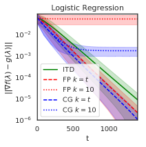
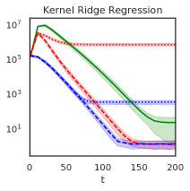
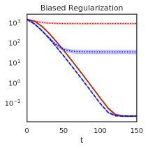
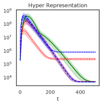
Figure 1: Convergence of different hypergradient approximations, where $g(\lambda)$ is equal to $\nabla f_{t}(\lambda)$ for ITD and to $\hat{\nabla}f(\lambda)$ for CG and FP. Mean and standard deviation (shaded areas) are computed over 20 values of $\lambda$ sampled uniformly from $[\lambda_{\min},\lambda_{\max}]^{n}$.

In the first part of this section we focus on the hypergradient approximation error and show that the upper bounds presented in the previous section give a good estimate of the actual convergence behaviour of ITD and AID strategies on a variety of settings. In the second part we present a series of experiments pertaining optimization on both the settings of hyperparameter optimization, as in problem (LABEL:mainprob1), and learning equilibrium models, as in problem (3). The algorithms have been implemented in PyTorch (Paszke et al., 2019). In the following, we shorthand AID-FP and AID-CG with FP and CG, respectively.

3.1 Hypergradient Approximation

In this section, we consider several problems of type (LABEL:mainprob1) with synthetic generated data (see Section C.1 for more details) where $D=(X,y)$ and $D^{\prime}=(X^{\prime},y^{\prime})$ are the training and validation sets respectively, with $X\in\mathbb{R}^{n_{e}\times p}$, $X^{\prime}\in\mathbb{R}^{n^{\prime}_{e}\times p}$, being $n_{e},n^{\prime}_{e}$ the number of examples in each set and $p$ the number of features. Specifically we consider the following settings, which are representative instances of relevant bilevel problems in machine learning.

Logistic Regression with $\ell_{2}$ Regularization (LR). This setting is similar to the one in Pedregosa (2016), but we introduce multiple regularization parameters:

$$f(\lambda) =\sum_{(x_{e},y_{e})\in D^{\prime}}\psi(y_{e}x_{e}^{\top}w(\lambda)),$$

$$w(\lambda) =\operatorname*{argmin}_{w\in\mathbb{R}^{p}}\sum_{(x_{e},y_{e})\in D}\psi(y_{e}x_{e}^{\top}w)+\frac{1}{2}w^{\top}{\rm diag}(\lambda)w,$$

where $\lambda\in\mathbb{R}^{p}_{++}$, $\psi(x)=\log(1+e^{-x})$ and ${\rm diag}(\lambda)$ is the diagonal matrix formed by the elements of $\lambda$.

Kernel Ridge Regression (KRR). We extend the setting presented by Pedregosa (2016) considering a $p$-dimensional Gaussian kernel parameter $\gamma$ in place of the usual one:

$$f(\beta,\gamma) =\frac{1}{2}\lVert{y^{\prime}-K^{\prime}(\gamma)w(\beta,\gamma)}\rVert^{2},$$ (22)

$$w(\beta,\gamma) =\operatorname*{argmin}_{w\in\mathbb{R}^{n_{e}}}\frac{1}{2}w^{\top}\left(K(\gamma)+\beta I\right)w-w^{\top}y,$$

where $\beta\in(0,\infty)$, $\gamma\in\mathbb{R}^{p}_{++}$ and $K^{\prime}(\gamma)$, $K(\gamma)$ are respectively the validation and training kernel matrices (see Section C.1).

Table 1: Objective (test accuracy) values after $s$ gradient descent steps where $s$ is $1000$, $500$ and $4000$ for Parkinson, 20 newsgroup and Fashion MNIST respectively. Test accuracy values are in %. $k_{r}=10$ for Parkinson and 20 newsgroup while for Fashion MNIST $k_{r}=5$.

Parkinson
	$t=100$	$t=150$
ITD	2.39 (75.8)	2.11 (69.7)
FP $k=t$	2.37 (81.8)	2.20 (77.3)
CG $k=t$	2.37 (78.8)	2.20 (77.3)
FP $k=k_{r}$	2.71 (80.3)	2.60 (78.8)
CG $k=k_{r}$	2.33 (77.3)	2.02 (77.3)

20 newsgroup
$t=10$	$t=25$	$t=50$
1.08 (61.3)	0.97 (62.8)	0.89 (64.2)
1.03 (62.1)	1.02 (62.3)	0.84 (64.4)
0.93 (63.7)	0.78 (63.3)	0.64 (63.1)
$-$	0.94 (63.6)	0.97 (63.0)
$-$	0.82 (64.3)	0.75 (64.2)

Fashion MNIST
$t=5$	$t=10$
0.41 (84.1)	0.43 (83.8)
0.41 (84.1)	0.43 (83.8)
0.42 (83.9)	0.42 (84.0)
$-$	0.42 (83.9)
$-$	0.42 (84.0)

Biased Regularization (BR). Inspired by Denevi et al. (2019); Rajeswaran et al. (2019), we consider the following.

$$f(\lambda) =\frac{1}{2}\lVert{X^{\prime}w(\lambda)-y^{\prime}}\rVert^{2},$$

$$w(\lambda) =\operatorname*{argmin}_{w\in\mathbb{R}^{p}}\frac{1}{2}\lVert{Xw-y}\rVert^{2}+\frac{\beta}{2}\lVert{w-\lambda}\rVert^{2},$$

where $\beta\in\mathbb{R}_{++}$ and $\lambda\in\mathbb{R}^{p}$.

Hyper-representation (HR). The last setting, reminiscent of (Franceschi et al., 2018; Bertinetto et al., 2019), concerns learning a (common) linear transformation of the data and is formulated as

$$f(H) =\frac{1}{2}\lVert{X^{\prime}Hw(H)-y^{\prime}}\rVert^{2}$$

$$w(H) =\operatorname*{argmin}_{w\in\mathbb{R}^{d}}\frac{1}{2}\lVert{XHw-y}\rVert^{2}+\frac{\beta}{2}\lVert{w}\rVert^{2}$$

where $H\in\mathbb{R}^{p\times d}$ and $\beta\in\mathbb{R}_{++}$.

LR and KRR are high dimensional extensions of classical hyperperparameter optimization problems, while BR and HR, are typically encountered in multi-task/meta-learning as single task objectives. Note that Assumption B (i.e. $\Phi(\cdot,\lambda)$ is a contraction) can be satisfied for each of the aforesaid scenarios, since they all belong to case a of Section 2.1 (KRR, BR and HR also to case b).

We solve the lower-level problem in the same way for both ITD and AID methods. In particular, in LR we use the gradient descent method with optimal step size as in case a of Section 2.1, while for the other cases we use the heavy-ball method with optimal step size and momentum constants. Note that this last method is not a contraction in the original norm, but only in a suitable norm depending on the lower-level problem itself. To compute the exact hypergradient, we differentiate $f(\lambda)$ directly using RMAD for KRR, BR and HR, where the closed form expression for $w(\lambda)$ is available, while for LR we use CG with $t=k=2000$ in place of the (unavailable) analytic gradient.

Figure 1 shows how the approximation error is affected by the number of lower-level iterations $t$. As suggested by the iteration complexity bounds in Section 2, all the approximations, after a certain number of iterations, converge linearly to the true hypergradient. Furthermore, in line with our analysis (see Section 2.3), CG gives the best gradient estimate (on average), followed by FP, while ITD performs the worst. For HR, the error of all the methods increases significantly at the beginning, which can be explained by the fact that the heavy ball method is not a contraction in the original norm and may diverge at first. CG $k=10$ outperforms FP $k=10$ on 3 out of 4 settings but both remain far from convergence.

3.2 Bilevel Optimization

In this section, we aim to solve instances of the bilevel problem (LABEL:mainprob) in which $\lambda$ has a high dimensionality.

Kernel Ridge Regression on Parkinson. We take $f(\beta,\gamma)$ as defined in problem (22) where the data is taken from the UCI Parkinson dataset (Little et al., 2008), containing 195 biomedical voice measurements (22 features) from people with Parkinson’s disease. To avoid projections, we replace $\beta$ and $\gamma$ respectively with $\exp(\beta)$ and $\exp(\gamma)$ in the RHS of the two equations in (22). We split the data randomly into three equal parts to make the train, validation and test sets.

Logistic Regression on 20 Newsgroup. This dataset contains 18000 news divided in 20 topics and the features consist in 101631 tf-idf sparse vectors. We split the data randomly into three equal parts for training, validation and testing. We aim to solve the bilevel problem

$$\begin{gathered}\min_{\lambda\in\mathbb{R}^{p}}\mathrm{CE}(X^{\prime}w(\lambda),y^{\prime})\\ w(\lambda)=\operatorname*{argmin}_{w\in\mathbb{R}^{p\times c}}\mathrm{CE}(Xw,y)+\frac{1}{2cp}\sum_{i=1}^{c}\sum_{j=1}^{p}\exp(\lambda_{j})w_{ij}^{2}\end{gathered}$$

where $\mathrm{CE}$ is the average cross-entropy loss, $c=20$ and $p=101631$. To improve the performance, we use warm-starts on the lower-level problem, i.e. we take $w_{0}(\lambda_{i})=w_{t}(\lambda_{i-1})$ for all methods, where $(\lambda_{i})_{i=1}^{s}$ are the upper-level iterates.

Training Data Optimization on Fashion MNIST. Similarly to (Maclaurin et al., 2015), we optimize the features of a set of 10 training points, each with a different class label on the Fashion MNIST dataset (Xiao et al., 2017). More specifically we define the bilevel problem as

$$\begin{gathered}\min_{X\in\mathbb{R}^{c\times p}}\mathrm{CE}(X^{\prime}w(X),y^{\prime})\\[-3.44444pt] w(X)=\arg\min_{w\in\mathbb{R}^{p\times c}}\mathrm{CE}(Xw,y)+\frac{\beta}{2cp}\lVert{w}\rVert^{2}\end{gathered}$$

where $\beta=1$, $c=10$, $p=784$, $y=(0,\dots,c)^{\top}$ and $(X^{\prime},y^{\prime})$ contains the usual training set.

We solve each problem using (hyper)gradient descent with fixed step size selected via grid search (additional details are provided in Section C.2). The results in Table 1 show the upper-level objective and test accuracy both computed on the approximate lower-level solution $w_{t}(\lambda)$ after bilevel optimization. For Parkinson and Fashion MNIST, there is little difference among the methods for a fixed $t$. For 20 newsgroup, CG $k=t$ reaches the lowest objective value, followed by CG $k=10$. We recall that for ITD we have cost in memory which is linear in $t$ and that, in the case of 20 newsgroup for some $t$ between $50$ and $100$, this cost exceeded the 11GB on the GPU. AID methods instead, require little memory and, by setting $k<t$, yield similar or even better performance at a lower computation time. Finally, we stress that since the upper-level objective is nonconvex, possibly with several minima, gradient descent with a more precise estimate of the hypergradient may get more easily trapped in a bad local minima.

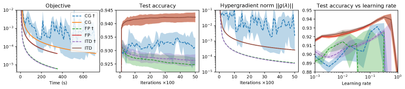
Figure 2: Experiments on EQM problems. Mean (solid or dashed lines) and point-wise minimum-maximum range (shaded regions) across 5 random seeds that only control the initialization of $\lambda$. The estimated hypergradient $g(\lambda)$ is equal to $\nabla f_{t}(\lambda)$ for ITD and $\hat{\nabla}f(\lambda)$ for AID. We used $t=k=20$ for all methods and Nesterov momentum for optimizing $\lambda$, applying a projection operator at each iteration except for the methods marked with ${\dagger}$. When performing projection, the curves produced by the three approximation schemes mostly overlap, indicating essentially the same performance (although at a different computational cost).

Equilibrium Models. Our last set of experiments investigates the behaviour of the hypergradient approximation methods on a simple instance of EQM (see problem (3)) on non-structured data. EQM are an attractive class of models due to their mathematical simplicity, enhanced interpretability and memory efficiency. A number of works (Miller & Hardt, 2019; Bai et al., 2019) have recently shown that EQMs can perform on par with standard deep nets on a variety of complex tasks, renewing the interest in these kind of models.

We use a subset of $n_{e}=5000$ instances randomly sampled from the MNIST dataset as training data and employ a multiclass logistic classifier paired with a cross-entropy loss. We picked a small training set and purposefully avoided stochastic optimization methods to better focus on issues related to the computation of the hypergradients itself, avoiding the introduction of other sources of noise. We parametrize $\phi_{i}$ as

$$\phi_{i}(w_{i},\gamma)=\tanh(Aw_{i}+Bx_{i}+c)\quad\text{for}\;1\leq i\leq n_{e}$$ (23)

where $x_{i}\in\mathbb{R}^{p}$ is the $i$-th example, $w_{i}\in\mathbb{R}^{h}$ and $\gamma=(A,B,C)\in\mathbb{R}^{h\times h}\times\mathbb{R}^{h\times p}\times\mathbb{R}^{h}$. Such a model may be viewed as a (infinite layers) feed-forward neural network with tied weights or as a recurrent neural network with static inputs. Additional experiments with convolutional equilibrium models may be found in Appendix C.3. Imposing $\lVert{A}\rVert<1$ ensures that the transition functions (23), and hence $\Phi$, are contractions. This can be achieved during optimization by projecting the singular values of $A$ onto the interval $[0,1-\varepsilon]$ for $\varepsilon>0$. We note that regularizing the norm of $\partial_{1}\phi_{i}$ or adding $L_{1}$ or $L_{\infty}$ penalty terms on $A$ may encourage, but does not strictly enforce, $\lVert{A}\rVert<1$.

We conducted a series of experiments to ascertain the importance of the contractiveness of the map $\Phi$, as well as to understand which of the analysed methods is to be preferred in this setting. Since here $\partial_{1}\Phi$ is not symmetric, the conjugate gradient method must be applied on the normal equations of problem (15). We set $h=200$ and use $t=20$ fixed-point iterations to solve the lower-level problem in all the experiments. The first three plots of Figure 2 report training objectives, test accuracies and norms of the estimated hypergradient for each of the three methods, either applying or not the constraint on $A$, while the last explores the sensitivity of the methods to the choice of the learning rate. Unconstrained runs are marked with ${\dagger}$. Referring to the rightmost plot, it is clear (large shaded regions) that not constraining the spectral norm results in unstable behaviour of the “memory-less” AID methods (green and blue lines) for all but a few learning rates, while ITD (violet), as expected, suffers comparatively less. On the contrary, when $\lVert{A}\rVert<1$ is enforced, all the approximation methods are successful and stable, with FP to be preferred being faster then CG on the normal equations and requiring substantially less memory than ITD. As a side note, referring to Figure 2 left and center-left, we observe that projecting onto the spectral ball acts as powerful regularizer, in line with the findings of Sedghi et al. (2019).

4 Conclusions

We studied a general class of bilevel problems where at the lower-level we seek for a solution to a parametric fixed point equation. This formulation encompasses several learning algorithms recently considered in the literature. We established results on the iteration complexity of two strategies to compute the hypergradient (ITD and AID) under the assumption that the fixed point equation is defined by a contraction mapping. Our practical experience with these methods on a number of bilevel problems indicates that there is a trade-off between the methods, with AID based on the conjugate gradient method being preferable due to a potentiality better approximation of the hypergradient and lower space complexity. When the contraction assumption is not satisfied, however, our experiments on equilibrium models suggest that ITD is more reliable than AID methods. In the future, it would be valuable to extend the ideas presented here to other challenging machine learning scenarios not covered by our theoretical analysis. These include bilevel problems in which the lower-level is only locally contactive, nonsmooth, possibly nonexpansive or can only be solved via a stochastic procedure. At the same time, there is a need to clarify the tightness of the iteration complexity bounds presented here.

Acknowledgments.

This work was supported in part by a grant from SAP SE.

Appendix

The Appendix is organized as follows.

• Appendix A presents the proofs of the results stated in Section 2.

• Appendix B specializes the bounds in Section 2 in the case where the lower-level solution can be written as the fixed point of a one step gradient descent map.

• Appendix C presents the details of the experiments in Section 3 and additional results.

Appendix A Proofs of the Results in Section 2

In this section we provide complete proofs of the results presented in the main body, which are restated here for the convenience of the reader. We also report few necessary additional results.

Theorem A.1.

(Differentiability of $f$). Consider problem (LABEL:mainprob) and suppose that Assumption Ai-ii holds. Then $w(\cdot)$ and $f(\cdot)$ are differentiable on $\Lambda$ and, for every $\lambda\in\Lambda$

$$w^{\prime}(\lambda) =(I-\partial_{1}\Phi(w(\lambda),\lambda))^{-1}\partial_{2}\Phi(w(\lambda),\lambda)$$ (24)

$$\nabla{f}(\lambda) =\nabla_{2}E(w(\lambda),\lambda)+w^{\prime}(\lambda)^{\top}\nabla_{1}E(w(\lambda),\lambda).$$ (25)

Proof.

The function $G(w,\lambda):=w-\Phi(w,\lambda)$ is continuously differentiable on $\mathbb{R}^{d}\times\Lambda$. Then, we have

$$\partial_{1}G(w(\lambda),\lambda)=I-\partial_{1}\Phi(w(\lambda),\lambda),$$

which is invertible due to Assumption Aii. Thus, since $G(w(\lambda),\lambda)=0$, the implicit function theorem yields that $w(\lambda)$ is continuously differentiable with derivative

$$w^{\prime}(\lambda) =\partial_{1}G(w(\lambda),\lambda)^{-1}\partial_{2}G(w(\lambda),\lambda)$$

$$=(I-\partial_{1}\Phi(w(\lambda),\lambda))^{-1}\partial_{2}\Phi(w(\lambda),\lambda).$$

Finally, (25) follows from the chain rule for differentiation. ∎

Corollary A.1.

Suppose that in problem (LABEL:mainprob1), the function $\ell\colon\mathbb{R}^{d}\times\Lambda\to\mathbb{R}$ is twice continuously differentiable and strongly convex w.r.t. the first variable. Let $\alpha\colon\Lambda\to\mathbb{R}_{++}$ be a differentiable function. Then the conclusions of Theorem A.1 hold and

$$(\forall\,\lambda\in\Lambda)\quad w^{\prime}(\lambda)=-\nabla^{2}_{1}\ell(w,\lambda)^{-1}\nabla_{21}^{2}\ell(w(\lambda),\lambda).$$

Proof.

Define $\Phi(w,\lambda)=w-\alpha(\lambda)\nabla_{1}\ell(w,\lambda)$. Then, Fermat’s rule for the lower-problem in (LABEL:mainprob1) yields that $w(\lambda)$ is a fixed point for $\Phi(\cdot,\lambda)$, while $I-\partial_{1}\Phi(w(\lambda),\lambda)$ is invertible since

$$I-\partial_{1}\Phi(w(\lambda),\lambda)=\alpha(\lambda)\nabla^{2}_{1}\ell(w,\lambda)$$

and $\alpha(\lambda)\neq 0$. Therefore, Theorem A.1 applies and, since $\partial_{2}\Phi(w(\lambda),\lambda)=-\alpha(\lambda)\nabla^{2}_{21}\ell(w(\lambda),\lambda)$, (24) yields $w^{\prime}(\lambda)=-\frac{\alpha(\lambda)}{\alpha(\lambda)}\nabla^{2}_{1}\ell(w,\lambda)^{-1}\nabla_{21}^{2}\ell(w(\lambda),\lambda)$. ∎

See 2.2

Proof.

Let $\lambda\in\Lambda$ and $w\in\mathbb{R}^{d}$. Since $\Phi(\cdot,\lambda)$ is Lipschitz continuous with constant $q_{\lambda}$, it follows that

$$\lVert{\partial_{1}\Phi(w,\lambda)}\rVert\leq q_{\lambda}<1.$$ (26)

Therefore,

$$\sum_{k=0}^{\infty}\lVert{\partial_{1}\Phi(w,\lambda)}\rVert^{k}\leq\sum_{k=0}^{\infty}q_{\lambda}^{k}=\frac{1}{1-q_{\lambda}}.$$

Thus, $I-\partial_{1}\Phi(w,\lambda)$ is invertible and $\sum_{k=0}^{\infty}\partial_{1}\Phi(w,\lambda)^{k}=(I-\partial_{1}\Phi(w,\lambda))^{-1}$ and the bound follows. ∎

In the following technical lemma we give two results which are fundamental for the proofs of the ITD bound (Theorem 2.1) and the AID-FP bound (Theorem 2.4). The first result is standard (see (Polyak, 1987), Lemma 1, Section 2.2).

Lemma A.1.

Let $(u_{k})_{k\in\mathbb{N}}$ and $(\tau_{k})_{k\in\mathbb{N}}$ be two sequences of real non-negative numbers and let $q\in[0,\infty)$. Suppose that, for every $k\in\mathbb{N}$, with $k\geq 1$,

$$u_{k}\leq qu_{k-1}+\tau_{k-1}.$$ (27)

Then, the following hold.

1. If $(\tau_{k})_{k\in\mathbb{N}}\equiv\tau$, then $u_{k}\leq q^{k}u_{0}+\tau(1-q^{k})/(1-q)$.

2. If, for every integer $k\geq 1$, $\tau_{k}\leq q\tau_{k-1}$, then $u_{k}\leq q^{k}u_{0}+kq^{k-1}\tau_{0}$.

Proof.

Let $k\in\mathbb{N}$, with $k\geq 1$. Then, we have

$$u_{k} \leq qu_{k-1}+\tau_{k-1}$$

$$\leq q(qu_{k-2}+\tau_{k-2})+\tau_{k-1}$$

$$=q^{2}u_{k-2}+(\tau_{k-1}+q\tau_{k-2})$$

$$\;\;\vdots$$

$$\leq q^{k}u_{0}+\sum_{i=0}^{k-1}q^{i}\tau_{k-1-i}.$$ (28)

i: Suppose that $(\tau_{k})_{k\in\mathbb{N}}\equiv\tau$. Then it follows from (28) that $u_{k}\leq q^{k}u_{0}+\tau\sum_{i=0}^{k-1}q^{i}=q^{k}u_{0}+\tau(1-q^{k})/(1-q)$.

ii: Suppose that, for every integer $k\geq 1$, $\tau_{k}\leq q\tau_{k-1}$. Then, for every integers $k,i$ with $i\leq k-1$, we have $\tau_{k-1-i}\leq q^{k-1-i}\tau_{0}$, which substituted into (28) yields

$$u_{k}\leq q^{k}u_{0}+\sum_{i=0}^{k-1}q^{i}q^{k-1-i}\tau_{0}$$

and ii follows. ∎

See 2.1

Proof.

We assume that $(w_{t}(\lambda))_{t\in\mathbb{N}}$ is defined through the iteration

$$w_{t}(\lambda)=\Phi(w_{t-1}(\lambda),\lambda)$$ (29)

starting from $w_{0}(\lambda)=0\in\mathbb{R}^{d}$. Let $t\in\mathbb{N}$ with $t\geq 1$. Then, the mapping $\lambda\mapsto w_{t}(\lambda)$ is differentiable since, in view of (1), it is a composition of differentiable functions, whereas $w^{\prime}(\lambda)$ exists due to Theorem A.1. Differentiating the lower-level equation in (LABEL:mainprob) and the recursive equation in (29), we get

$$w^{\prime}_{t}(\lambda) =\partial_{1}\Phi(w_{t-1}(\lambda),\lambda)w^{\prime}_{t-1}(\lambda)+\partial_{2}\Phi(w_{t-1}(\lambda),\lambda)$$

$$w^{\prime}(\lambda) =\partial_{1}\Phi(w(\lambda),\lambda)w^{\prime}(\lambda)+\partial_{2}\Phi(w(\lambda),\lambda).$$ (30)

Therefore, we get

$$\lVert w^{\prime}_{t}(\lambda) -w^{\prime}(\lambda)\rVert$$

$$\leq\lVert{\partial_{1}\Phi(w_{t-1}(\lambda),\lambda)-\partial_{1}\Phi(w(\lambda),\lambda)}\rVert\lVert{w^{\prime}(\lambda)}\rVert$$

$$\qquad+\lVert{\partial_{1}\Phi(w_{t-1}(\lambda),\lambda)}\rVert\lVert{w^{\prime}_{t-1}(\lambda)-w^{\prime}(\lambda)}\rVert$$

$$\qquad+\lVert{\partial_{2}\Phi(w_{t-1}(\lambda),\lambda)-\partial_{2}\Phi(w(\lambda),\lambda)}\rVert$$

and hence, we derive from Assumption Aiii, Assumption B, equation (4) and Lemmas 2.1 and 2.2, that

$$\lVert w^{\prime}_{t}(\lambda) -w^{\prime}(\lambda)\rVert$$

$$\leq(\nu_{2,\lambda}+\nu_{1,\lambda}L_{\Phi,\lambda}/(1-q_{\lambda}))\lVert{w_{t-1}(\lambda)-w(\lambda)}\rVert$$

$$\qquad+q_{\lambda}\lVert{w^{\prime}_{t-1}(\lambda)-w^{\prime}(\lambda)}\rVert.$$

Then, setting $p:=\nu_{2,\lambda}+\nu_{1,\lambda}L_{\Phi,\lambda}/(1-q_{\lambda})$, $\Delta_{t}:=\lVert{w_{t}(\lambda)-w(\lambda)}\rVert$ and $\Delta^{\prime}_{t}:=\lVert{w^{\prime}_{t}(\lambda)-w^{\prime}(\lambda)}\rVert$, we get

$$\Delta_{t}\leq q_{\lambda}\Delta_{t-1}\quad\text{and}\quad\Delta^{\prime}_{t}\leq q_{\lambda}\Delta^{\prime}_{t-1}+p\Delta_{t-1}.$$

Therefore, it follows from Lemma A.1ii (with $u_{t}=\Delta^{\prime}_{t}$ and $\tau_{t}=p\Delta_{t}$) that

$$\Delta^{\prime}_{t}\leq q_{\lambda}^{t}\Delta^{\prime}_{0}+tq_{\lambda}^{t-1}p\Delta_{0}\leq\frac{L_{\Phi,\lambda}}{1-q_{\lambda}}q_{\lambda}^{t}+pD_{\lambda}tq_{\lambda}^{t-1},$$

where in the last inequality we used the bounds (see (30) and Lemmas 2.1 and 2.2)

$$\Delta_{0} =\lVert{w(\lambda)-w_{0}(\lambda)}\rVert=\lVert{w(\lambda)}\rVert\leq D_{\lambda}$$

$$\Delta^{\prime}_{0} =\lVert{w^{\prime}(\lambda)-w^{\prime}_{0}(\lambda)}\rVert=\lVert{w^{\prime}(\lambda)}\rVert\leq\frac{L_{\Phi,\lambda}}{1-q_{\lambda}}.$$ (31)

Recalling the definitions of $p$ and $\Delta^{\prime}_{t}$, (7) follows. ∎

See 2.1

Proof.

It follows from the definitions of $f_{t}$ and $f$ in Algorithm 1 and (LABEL:mainprob) respectively and the chain rule for differentiation that

$$\nabla f_{t}(\lambda) =\nabla_{2}E(w_{t}(\lambda),\lambda)+w^{\prime}_{t}(\lambda)^{\top}\nabla_{1}E(w_{t}(\lambda),\lambda)$$

$$\nabla f(\lambda) =\nabla_{2}E(w(\lambda),\lambda)+w^{\prime}(\lambda)^{\top}\nabla_{1}E(w(\lambda),\lambda).$$

Therefore,

$$\lVert\nabla f_{t} (\lambda)-\nabla f(\lambda)\rVert$$

$$\leq\lVert{\nabla_{2}E(w_{t}(\lambda),\lambda)-\nabla_{2}E(w(\lambda),\lambda)}\rVert$$

$$\qquad+\lVert{w^{\prime}(\lambda)}\rVert\lVert{\nabla_{1}E(w_{t}(\lambda),\lambda)-\nabla_{1}E(w(\lambda),\lambda)}\rVert$$

$$\qquad+\lVert{w^{\prime}_{t}(\lambda)-w^{\prime}(\lambda)}\rVert\lVert{\nabla_{1}E(w_{t}(\lambda),\lambda)}\rVert.$$

Now, we note that $\lVert{w_{t}(\lambda)}\rVert\leq\lVert{w_{t}(\lambda)-w(\lambda)}\rVert+\lVert{w(\lambda)}\rVert\leq(q_{\lambda}^{t}+1)\lVert{w(\lambda)}\rVert\leq 2D_{\lambda}$. Therefore, it follows from Assumption Aiv and Lemmas 2.1 and 2.2 that

$$\lVert{\nabla f_{t}(\lambda)-\nabla f(\lambda)}\rVert\leq \left(\eta_{2,\lambda}+\eta_{1,\lambda}L_{\Phi,\lambda}/(1-q_{\lambda})\right)q_{\lambda}^{t}D_{\lambda}$$

$$+L_{E,\lambda}\lVert{w^{\prime}(\lambda)-w^{\prime}_{t}(\lambda)}\rVert,$$

where we used $\lVert{w_{t}(\lambda)-w(\lambda)}\rVert\leq q_{\lambda}^{t}\lVert{w_{0}(\lambda)-w(\lambda)}\rVert=q_{\lambda}^{t}\lVert{w(\lambda)}\rVert\leq q_{\lambda}^{t}D_{\lambda}$. Then, (8) follows from Proposition 2.1. ∎

Now we address the proofs related to the AID method described in Section 2.2.

See 2.2

Proof.

For the sake of brevity we set

$$A_{\lambda,t} =I-\partial_{1}\Phi(w_{t}(\lambda),\lambda)^{\top}\!\!\!, A_{\lambda} =I-\partial_{1}\Phi(w(\lambda),\lambda)^{\top}\!\!\!,$$

$$Z_{\lambda,t} =\partial_{2}\Phi(w_{t}(\lambda),\lambda), Z_{\lambda} =\partial_{2}\Phi(w(\lambda),\lambda),$$

$$b_{\lambda,t} =\nabla_{1}E(w_{t}(\lambda),\lambda), b_{\lambda} =\nabla_{1}E(w(\lambda),\lambda),$$

$$c_{\lambda,t} =\nabla_{2}E(w_{t}(\lambda),\lambda), c_{\lambda} =\nabla_{2}E(w(\lambda),\lambda).$$

It follows form Assumption Cii that $\lVert{w_{t}(\lambda)-w(\lambda)}\rVert\leq\rho_{\lambda}(t)\lVert{w(\lambda)}\rVert\leq\rho_{\lambda}(t)D_{\lambda}\leq D_{\lambda}$ and hence $\lVert{w_{t}(\lambda)}\rVert\leq\lVert{w_{t}(\lambda)-w(\lambda)}\rVert+\lVert{w(\lambda)}\rVert\leq 2D_{\lambda}$. Then the following upper bounds related to the above quantities follow from Assumptions Aiii-iv, equation (12) and Lemma 2.1.

$$\lVert{A_{\lambda,t}\!-\!A_{\lambda}}\rVert\leq\nu_{1,\lambda}\rho_{\lambda}(t)D_{\lambda},\ \lVert{Z_{\lambda,t}\!-\!Z_{\lambda}}\rVert\leq\nu_{2,\lambda}\rho_{\lambda}(t)D_{\lambda},$$

$$\lVert{b_{\lambda,t}-b_{\lambda}}\rVert\leq\eta_{1,\lambda}\rho_{\lambda}(t)D_{\lambda},\ \lVert{c_{\lambda,t}-c_{\lambda}}\rVert\leq\eta_{2,\lambda}\rho_{\lambda}(t)D_{\lambda},$$

$$\lVert{A_{\lambda,t}^{-1}}\rVert,\lVert{A_{\lambda}^{-1}}\rVert\leq\frac{1}{\mu_{\lambda}},\ \lVert{Z_{\lambda,t}}\rVert\leq L_{\Phi,\lambda},\ \lVert{b_{\lambda,t}}\rVert,\lVert{b_{\lambda}}\rVert\leq L_{E,\lambda}.$$

Now, setting $v_{t}(\lambda)=A_{\lambda,t}^{-1}b_{\lambda,t}$ and $v(\lambda)=A_{\lambda}^{-1}b_{\lambda}$, $\hat{\nabla}f(\lambda)$ and (9) can be written as

$$\hat{\nabla}f(\lambda)=c_{\lambda,t}+Z_{\lambda,t}^{\top}v_{t,k}(\lambda),\ \nabla f(\lambda)=c_{\lambda}+Z_{\lambda}^{\top}v(\lambda).$$

Then, we have

$$\lVert \hat{\nabla}f(\lambda)-\nabla f(\lambda)\rVert$$

$$=\lVert{c_{\lambda,t}+Z_{\lambda,t}^{\top}v_{t,k}(\lambda)-c_{\lambda}-Z_{\lambda}^{\top}v(\lambda)}\rVert$$

$$\leq\lVert{c_{\lambda,t}-c_{\lambda}}\rVert$$

$$\quad\ +\lVert{Z_{\lambda,t}^{\top}v_{t,k}(\lambda)-Z_{\lambda,t}^{\top}v(\lambda)+Z_{\lambda,t}^{\top}v(\lambda)-Z_{\lambda}^{\top}v(\lambda)}\rVert$$

$$\leq\lVert{c_{\lambda,t}-c_{\lambda}}\rVert$$

$$\quad\ +\lVert{Z_{\lambda,t}}\rVert\lVert{v_{t,k}(\lambda)-v(\lambda)}\rVert+\lVert{Z_{\lambda,t}-Z_{\lambda}}\rVert\lVert{v(\lambda)}\rVert$$

$$\leq\lVert{c_{\lambda,t}-c_{\lambda}}\rVert$$

$$\quad\ +\lVert{Z_{\lambda,t}}\rVert\lVert{v_{t,k}(\lambda)-v(\lambda)}\rVert\!+\!\lVert{Z_{\lambda,t}-Z_{\lambda}}\rVert\lVert{A_{\lambda}^{-1}}\rVert\lVert{b_{\lambda}}\rVert$$

$$\leq\left(\eta_{2,\lambda}+\frac{\nu_{2,\lambda}L_{E,\lambda}}{\mu_{\lambda}}\right)\rho_{\lambda}(t)D_{\lambda}+L_{\Phi,\lambda}\lVert{v_{t,k}(\lambda)-v(\lambda)}\rVert.$$

Moreover, it follows from Ciii that

$$\lVert{v_{t,k}(\lambda)-v(\lambda)}\rVert \leq\lVert{v_{t,k}(\lambda)-v_{t}(\lambda)}\rVert+\lVert{v_{t}(\lambda)-v(\lambda)}\rVert$$

$$\leq\sigma_{\lambda}(k)\frac{L_{E,\lambda}}{\mu_{\lambda}}+\lVert{v_{t}(\lambda)-v(\lambda)}\rVert.$$

Finally, we have

$$\lVert v_{t}(\lambda) -v(\lambda)\rVert$$

$$\leq\lVert{A_{\lambda,t}^{-1}b_{\lambda,t}-A_{\lambda,t}^{-1}b_{\lambda}+A_{\lambda,t}^{-1}b_{\lambda}-A_{\lambda}^{-1}b_{\lambda}}\rVert$$

$$\leq\lVert{A_{\lambda,t}^{-1}}\rVert\lVert{b_{\lambda,t}-b_{\lambda}}\rVert+\lVert{b_{\lambda}}\rVert\lVert{A_{\lambda,t}^{-1}-A_{\lambda}^{-1}}\rVert$$

$$\leq\frac{\eta_{1,\lambda}\rho_{\lambda}(t)D_{\lambda}}{\mu_{\lambda}}+L_{E,\lambda}\lVert{A_{\lambda,t}^{-1}-A_{\lambda}^{-1}}\rVert$$

$$\leq\frac{\eta_{1,\lambda}\rho_{\lambda}(t)D_{\lambda}}{\mu_{\lambda}}+L_{E,\lambda}\lVert{A_{\lambda,t}^{-1}}\rVert\lVert{A_{\lambda}-A_{\lambda,t}}\rVert\lVert{A_{\lambda}^{-1}}\rVert$$

$$\leq\frac{\eta_{1,\lambda}\rho_{\lambda}(t)D_{\lambda}}{\mu_{\lambda}}+\frac{L_{E,\lambda}\nu_{1,\lambda}\rho_{\lambda}(t)D_{\lambda}}{\mu_{\lambda}^{2}}.$$

Combining all together we get (13). As regards the second part of the statement, if Assumption B is satisfied, then, in view of Lemma 2.2, we can take $\mu_{\lambda}=1-q_{\lambda}$ in (12) and obtain (14). ∎

The following two propositions allow us to derive the refined iteration complexity bound for AID-FP.

Proposition A.1.

Suppose that (19) holds. Let $\lambda\in\Lambda,t\in\mathbb{N}$. Let $u_{t,0}(\lambda)=0\in\mathbb{R}^{d\times n}$ and for every integer $k\geq 1$,

$$u_{t,k}(\lambda)=\partial_{1}\Phi(w_{t}(\lambda),\lambda)u_{t,k-1}(\lambda)+\partial_{2}\Phi(w_{t}(\lambda),\lambda).$$

Then, for every $k\in\mathbb{N}$,

$$u_{t,k}(\lambda)^{\!\top}\nabla_{1}E(w_{t}(\lambda),\lambda)=\partial_{2}\Phi(w_{t}(\lambda),\lambda)^{\top}\!v_{t,k}(\lambda).$$ (32)

Proof.

We set $Y=\partial_{1}\Phi(w_{t}(\lambda),\lambda)\in\mathbb{R}^{d\times d}$, $C=\partial_{2}\Phi(w_{t}(\lambda),\lambda)\in\mathbb{R}^{d\times n}$, and $b=\nabla_{1}E(w_{t}(\lambda),\lambda)\in\mathbb{R}^{d}$. Let $k\in\mathbb{N}$, $k\geq 1$. Then,

$$u_{t,k}(\lambda) =Yu_{t,k-1}(\lambda)+C$$

$$=Y^{2}u_{t,k-2}(\lambda)+(1+Y)C$$

$$\;\;\vdots$$

$$=Y^{k}u_{t,0}(\lambda)+\sum_{i=0}^{k-1}Y^{i}C$$

$$=\sum_{i=0}^{k-1}Y^{i}C.$$

In the same way, it follows from (19) that $v_{t,k}(\lambda)=Y^{\top}v_{t,k-1}(\lambda)+b=\sum_{i=0}^{k-1}(Y^{\top})^{i}b$. Therefore, we have

$$u_{t,k}(\lambda)^{\top}b =C^{\top}\left(\sum_{i=0}^{k-1}Y^{i}\right)^{\top}b$$

$$=C^{\top}\sum_{s=i}^{k-1}(Y^{\top})^{i}b$$

$$=C^{\top}v_{t,k}(\lambda)$$

and the statement follows. ∎

Using Proposition A.1, for AID-FP we can write

$$\hat{\nabla}{f}(\lambda)\!=\!\nabla_{\!2}E(w_{t}(\lambda),\lambda)+u_{t,k}(\lambda)^{\!\top}\!\nabla_{\!1}E(w_{t}(\lambda),\lambda).$$ (33)

Then a result similar to Proposition 2.1 can be derived.

Proposition A.2.

Suppose that Assumption Aiiii and Assumption B hold. Let $\lambda\in\Lambda$ and $(u_{t,k}(\lambda))_{k\in\mathbb{N}}$ be defined as in Proposition A.1. Then, for every $t,k\in\mathbb{N}$, with $t\geq 1$,

$$\lVert{u_{t,k}(\lambda)-w^{\prime}(\lambda)}\rVert\\ \leq\left(\!\nu_{2,\lambda}+\nu_{1,\lambda}\frac{L_{\Phi,\lambda}}{(1-q_{\lambda})}\!\right)\!\frac{D_{\lambda}(1-q_{\lambda}^{k})}{1-q_{\lambda}}\rho_{\lambda}(t)+\frac{L_{\Phi,\lambda}}{1-q_{\lambda}}q_{\lambda}^{k}.$$

Proof.

Let $t,k\in\mathbb{N}$, with $t,k\geq 1$. Recalling that

$$u_{t,k}(\lambda)=\partial_{1}\Phi(w_{t}(\lambda),\lambda)u_{t,k-1}(\lambda)+\partial_{2}\Phi(w_{t}(\lambda),\lambda)$$

$$w^{\prime}(\lambda)=\partial_{1}\Phi(w(\lambda),\lambda)w^{\prime}(\lambda)+\partial_{2}\Phi(w(\lambda),\lambda)$$

we can bound the norm of the difference as follows

$$\lVert u_{t,k}(\lambda) -w^{\prime}(\lambda)\rVert$$

$$\leq \lVert{\partial_{1}\Phi(w_{t}(\lambda),\lambda)-\partial_{1}\Phi(w(\lambda),\lambda)}\rVert\lVert{w^{\prime}(\lambda)}\rVert$$

$$+\lVert{\partial_{1}\Phi(w_{t}(\lambda),\lambda)}\rVert\lVert{u_{t,k-1}(\lambda)-w^{\prime}(\lambda)}\rVert$$

$$+\lVert{\partial_{2}\Phi(w_{t}(\lambda),\lambda)-\partial_{2}\Phi(w(\lambda),\lambda)}\rVert$$

$$\leq (\nu_{2,\lambda}+\nu_{1,\lambda}L_{\Phi,\lambda}/(1-q_{\lambda}))\lVert{w_{t}(\lambda)-w(\lambda)}\rVert$$

$$+q_{\lambda}\lVert{u_{t,k-1}(\lambda)-w^{\prime}(\lambda)}\rVert,$$

which gives a recursive inequality. Then, setting $p:=\nu_{2,\lambda}+\nu_{1,\lambda}L_{\Phi,\lambda}/(1-q_{\lambda})$, $\Delta_{t}:=\lVert{w_{t}(\lambda)-w(\lambda)}\rVert$ and $\hat{\Delta}^{\prime}_{k}:=\lVert{u_{t,k}(\lambda)-w^{\prime}(\lambda)}\rVert$, we have

$$\hat{\Delta}^{\prime}_{k}\leq q_{\lambda}\hat{\Delta}^{\prime}_{k-1}+p\Delta_{t}.$$

Therefore, it follows from Lemma A.1i with $\tau=p\Delta_{t}$, that

$$\hat{\Delta}^{\prime}_{k} \leq q_{\lambda}^{k}\hat{\Delta}^{\prime}_{0}+p\Delta_{t}\frac{1-q_{\lambda}^{k}}{1-q_{\lambda}}$$

$$\leq\frac{L_{\Phi,\lambda}}{1-q_{\lambda}}q_{\lambda}^{k}+pD_{\lambda}\rho_{\lambda}(t)\frac{1-q_{\lambda}^{k}}{1-q_{\lambda}},$$

where in the last inequality we used Assumption Cii and (see (31)) $\hat{\Delta}^{\prime}_{0}=\lVert{u_{t,0}(\lambda)-w^{\prime}(\lambda)}\rVert=\lVert{w^{\prime}(\lambda)}\rVert\leq L_{\Phi,\lambda}/(1-q_{\lambda})$. The statement follows. ∎

See 2.4

Proof.

Let $t\in\mathbb{N}$ with $t\geq 1$ and let $(u_{t,k}(\lambda))_{k\in\mathbb{N}}$ be defined as in Proposition A.1. Then, the difference between exact and approximate gradients can be bound as follows

$$\lVert\hat{\nabla}f(\lambda) -\nabla f(\lambda)\rVert$$

$$\leq \lVert{\nabla_{2}E(w_{t}(\lambda),\lambda)-\nabla_{2}E(w(\lambda),\lambda)}\rVert$$

$$+\lVert{w^{\prime}(\lambda)}\rVert\lVert{\nabla_{1}E(w_{t}(\lambda),\lambda)-\nabla_{1}E(w(\lambda),\lambda)}\rVert$$

$$+\lVert{w^{\prime}(\lambda)-u_{t,k}(\lambda)}\rVert\lVert{\nabla_{1}E(w_{t}(\lambda),\lambda)}\rVert.$$

Now note that $\lVert{w_{t}(\lambda)}\rVert\leq\lVert{w_{t}(\lambda)-w(\lambda)}\rVert+\lVert{w(\lambda)}\rVert\leq(\rho_{\lambda}(t)+1)\lVert{w(\lambda)}\rVert\leq 2D_{\lambda}$. Then it follows from the assumptions and Lemmas 2.2 and 2.1 that

$$\lVert{\nabla f(\lambda)-\hat{\nabla}{f}(\lambda)}\rVert\leq \left(\eta_{2,\lambda}+\frac{\eta_{1,\lambda}L_{\Phi,\lambda}}{1-q_{\lambda}}\right)\rho_{\lambda}(t)D_{\lambda}$$

$$+L_{E,\lambda}\lVert{u_{t,k}(\lambda)-w^{\prime}(\lambda)}\rVert,$$

and the last term can be bounded using Proposition A.2. ∎

Appendix B Gradient Descent as a Contraction Map

Consider problem (LABEL:mainprob1) and take

$$\Phi(w,\lambda)=w-\alpha(\lambda)\nabla_{1}\ell(w,\lambda),$$

where $\ell\colon\mathbb{R}^{d}\times\Lambda\to\mathbb{R}$ is twice continuously differentiable and, for every $\lambda\in\Lambda$,

1. $\ell(\cdot,\lambda)$ is $\mu_{\ell}(\lambda)$-strongly convex and $L_{\ell}(\lambda)$-Lipschitz smooth, with $\mu_{\ell}(\lambda)>0$ and $L_{\ell}(\lambda)>0$.

2. $\alpha\colon\Lambda\subset\mathbb{R}^{n}\to\mathbb{R}_{++}$ is differentiable.

Then, if $\alpha(\lambda)\in(0,2/L_{\ell}(\lambda))$, $\Phi(\cdot,\lambda)$ is a contraction with constant $q_{\lambda}=\max\{1-\alpha(\lambda)\mu_{\ell}(\lambda),\alpha(\lambda)L_{\ell}(\lambda)-1\}$. The optimal choice of the step-size leads to set $\alpha(\lambda)=2/(L_{\ell}(\lambda)+\mu_{\ell}(\lambda))$ giving

$$q_{\lambda}=\frac{L_{\ell}(\lambda)-\mu_{\ell}(\lambda)}{L_{\ell}(\lambda)+\mu_{\ell}(\lambda)}=\frac{\kappa(\lambda)-1}{\kappa(\lambda)+1},$$

where $\kappa(\lambda)=L_{\ell}(\lambda)/\mu_{\ell}(\lambda)$ is the condition number of the lower level problem in (LABEL:mainprob1). Note that, for every $t\in\mathbb{N}$ and $\lambda\in\Lambda$,

$$\mu_{\ell}(\lambda)I\preccurlyeq\nabla_{1}^{2}\ell(w_{t}(\lambda),\lambda)\preccurlyeq L_{\ell}(\lambda)I$$ (34)

hence the condition number of $\nabla_{1}^{2}\ell(w_{t}(\lambda),\lambda)$ is smaller than $\kappa(\lambda)$.

We can write the derivatives of $\Phi$ as:

$$\partial_{2}\Phi(w,\lambda) =-\nabla_{1}\ell(w,\lambda)\nabla\alpha(\lambda)^{\top}-\alpha(\lambda)\nabla^{2}_{21}\ell(w,\lambda)$$ (35)

$$\partial_{1}\Phi(w,\lambda) =I-\alpha(\lambda)\nabla^{2}_{1}\ell(w,\lambda)$$ (36)

Remark B.1.

When evaluated in $(w(\lambda),\lambda)$, one does not need $\nabla\alpha(\lambda)$ for (35), because the first term on the r.h.s of eq. 35 is $0$:

$$\partial_{2}\Phi(w(\lambda),\lambda)=-\alpha(\lambda)\nabla^{2}_{21}\ell(w(\lambda),\lambda).$$

From the remark it follows that $\lVert{\partial_{2}\Phi(w(\lambda),\lambda)}\rVert=\alpha(\lambda)\lVert{\nabla^{2}_{21}\ell(w(\lambda),\lambda)}\rVert$

Furthermore, if we assume $\nabla^{2}_{1}\ell(\cdot,\lambda)$ is $\hat{\rho}_{1,\lambda}$-Lipschitz and $\nabla^{2}_{21}\ell(\cdot,\lambda)$ is $\hat{\rho}_{2,\lambda}$-Lipschitz then, calling $\Delta_{\partial_{1}\Phi}:=\lVert{\partial_{1}\Phi(w_{1},\lambda)-\partial_{1}\Phi(w_{2},\lambda)}\rVert$ and $\Delta_{\partial_{2}\Phi}:=\lVert{\partial_{2}\Phi(w_{1},\lambda)-\partial_{2}\Phi(w_{2},\lambda)}\rVert$ we have:

$$\Delta_{\partial_{1}\Phi} =\lVert{\alpha(\lambda)\left(\nabla^{2}_{1}\ell(w_{1},\lambda)-\nabla^{2}_{1}\ell(w_{2},\lambda)\right)}\rVert$$

$$\leq\alpha(\lambda)\hat{\rho}_{1,\lambda}\lVert{w_{1}-w_{2}}\rVert.$$

and

$$\Delta_{\partial_{2}\Phi} = \lVert\left(\nabla_{1}\ell(w_{1},\lambda)-\nabla_{1}\ell(w_{2},\lambda)\right)\nabla\alpha(\lambda)^{\top}$$

$$+\alpha(\lambda)\left(\nabla^{2}_{21}\ell(w_{1},\lambda)-\nabla^{2}_{21}\ell(w_{2},\lambda)\right)\rVert$$

$$\leq (L_{\ell}(\lambda)\lVert{\nabla\alpha(\lambda)}\rVert+\alpha(\lambda)\hat{\rho}_{2,\lambda})\lVert{w_{1}-w_{2}}\rVert.$$

Thus, Assumption Aiii holds with $\nu_{1,\lambda}=\alpha(\lambda)\hat{\rho}_{1,\lambda}$ and $\nu_{2,\lambda}=L_{\ell}(\lambda)\lVert{\nabla\alpha(\lambda)}\rVert+\alpha(\lambda)\hat{\rho}_{2,\lambda}$. Moreover, if we pick $L_{\ell,\lambda}$ such that $\lVert{\nabla^{2}_{21}\ell(w(\lambda),\lambda)}\rVert\leq L_{\ell,\lambda}$, then Theorems 2.1,2.2 and 2.4 hold with

$$q_{\lambda} =\max\{1-\alpha(\lambda)\mu_{\ell}(\lambda),\alpha(\lambda)L_{\ell}(\lambda)-1\}$$

$$c_{1}(\lambda) :=\left(\eta_{2,\lambda}+\frac{\eta_{1,\lambda}\alpha(\lambda)L_{\ell,\lambda}}{1-q_{\lambda}}\right)D_{\lambda}$$

$$c_{2}(\lambda) :=\left(L_{\ell}(\lambda)\lVert{\nabla\alpha(\lambda)}\rVert+\alpha(\lambda)\hat{\rho}_{2,\lambda}\right)L_{E,\lambda}\,D_{\lambda}$$

$$\ \ +\frac{\hat{\rho}_{1,\lambda}\alpha(\lambda)^{2}L_{\ell,\lambda}L_{E,\lambda}\,D_{\lambda}}{1-q_{\lambda}}$$

$$c_{3}(\lambda) :=\frac{L_{E,\lambda}\,\alpha(\lambda)\lVert{\nabla^{2}_{21}\ell(w(\lambda),\lambda)}\rVert}{(1-q_{\lambda})}.$$

Given Remark B.1 and to avoid additional complexity of the algorithm, we can consider replacing $\partial_{2}\Phi(w,\lambda)$ with $\hat{\partial}_{2}\Phi(w,\lambda)=-\alpha(\lambda)\nabla^{2}_{21}\ell(w,\lambda)$ in the expression for both $\nabla f_{t}(\lambda)$ and $\hat{\nabla}f(\lambda)$. We apply this change in all the experiments of case (LABEL:mainprob1).

Appendix C Experiments

C.1 Hypergradient Approximation

In this section we provide details for the experiments in Section 3.1.

We define the train and validation kernel matrices in (22) as follows:

$$K^{\prime}(\gamma)_{i,j} =\exp\left[-\left(X^{\prime}_{i}-X_{j}\right)^{\top}{\rm diag}(\gamma)\left(X^{\prime}_{i}-X_{j}\right)\right]$$

$$K(\gamma)_{i,j} =\exp\left[-\left(X_{i}-X_{j}\right)^{\top}{\rm diag}(\gamma)\left(X_{i}-X_{j}\right)\right].$$

We generate synthetic data by sampling each element of $X$ and $X^{\prime}$ from a normal distribution. $y$ (and in the same way $y^{\prime}$) is subsequently obtained in the following ways for the different settings outlined in Section 3.1.

$$y =sign(Xw_{*}+m\epsilon)\quad\qquad$$ (LR)

$$y =Xw_{*}+m\epsilon\quad\qquad$$ (KRR)

$$y =X(w_{*}+b_{*})+m\epsilon\qquad$$ (BR)

$$y =XH_{*}w_{*}+m\epsilon\qquad$$ (HR)

where $sign$ is the elementwise sign function, each element of $\epsilon$, $w_{*}$ and $H_{*}$ is sampled from a normal distribution, $b_{*}=\mathbb{1}$, and $m=0.1$. $X$,$X^{\prime}$ have dimension $50\times 100$ while $H$ is a $100\times 200$ matrix. The results in Figure 1 report mean and std over $20$ values of $\lambda$ such that $\lambda_{i}\sim\mathcal{U}(\lambda_{\min},\lambda_{\max})$ for $1\leq i\leq n$ where $\mathcal{U}$ is the uniform distribution on the interval [$\lambda_{\min}$, $\lambda_{\max}$] which is $[0.01,10]$, $[0.0005,0.005]$, $[-5,5]$ and $[-1,1]$ respectively for LR, KRR, BR, HR. Furthemrmore we set $\beta=1$ for BR and $\beta=10$ for HR. $\lambda_{\min}$, $\lambda_{\max}$ and $\beta$ are selected as to make the expected lower-level problem difficult ($q_{\lambda}$ close to $1$).

We note that in Figure 1 the asymptotic error for KRR, BR and HR is considerably large. We suspect that this is due to the numerical error made by the hypergradient approximation procedures being larger than the one made when computing the exact hypergradient using the closed form expression of $w(\lambda)$. Indeed, we have observed that using double precision halves the asymptotic error, but we did not investigate further. Our theoretical analysis does not take this source of error into account since it assumes infinite precision arithmetic.

C.2 Bilevel Optimization

This section contains the details and some additional results on the experiments in Section 3.2 on problems of type (LABEL:mainprob1).

The average cross-entropy in 20 newsgroup and Fashion MNIST is defined as

$$\mathrm{CE}(Z,y)=-\frac{1}{|y|}\sum_{k=1}^{|y|}\sum_{i=1}^{c}\delta_{i,y_{k}}\log\left(\frac{e^{Z_{ki}}}{\sum_{j=1}^{c}e^{Z_{kj}}}\right)$$

where $Z_{k}\in\mathbb{R}^{c}$ $y_{k}\in\{0,\dots,c\}$ are respectively the prediction scores and the class label for the $k$-th example, $\delta_{i,y_{k}}$ equals $1$ when $i=y_{k}$ and $0$ otherwise and $|y|$ is the number of examples.

To solve the upper-level problem we use gradient descent with fixed step-size where the gradient is estimated using ITD or AID methods. In particular, we generate the sequence $(\lambda_{i})^{s}_{i}$ as follows:

$$\lambda_{i}=\lambda_{i-1}-\zeta g(\lambda_{i-1})$$

where $g(\lambda)=\nabla f_{t}(\lambda)$ for ITD and $g(\lambda)=\hat{\nabla}f(\lambda)$ for AID are computed respectively using Algorithm 1 and Algorithm 2 with $t$ and $k$ fixed throughout the optimization.

All methods compute $w_{t}(\lambda)$ using $t$-steps of the same algorithm solving the lower-level problem in (LABEL:mainprob1). In particular we use heavy ball with optimal constants for Parkinson and gradient descent with step-size manually chosen for the other two settings where it is harder to compute the optimal one. Specifically, we set the step-size to $10^{3}$ for 20 newsgroup and $10^{4}$ for Fashion MNSIT.

The initial parameter $\lambda_{0}$ is set to $(\beta_{0},\gamma_{0})=(0,-\log(p)\mathbb{1})$ for Parkinson, $0\in\mathbb{R}^{p}$ for 20 newsgroup and $X_{0}=0\in\mathbb{R}^{c\times p}$ for Fashion MNIST. Furthermore, the regularization parameter $\beta$ is set to $1$ for Fashion MNIST.

We choose the step-size $\zeta$ with a grid search over 30 values in a suitable interval for each problem, choosing the one bringing the lowest value of the approximate objective $f_{t}(\lambda_{s})=E(w_{t}(\lambda_{s}),\lambda_{s})$ where $s$ is equal to $1000$, $500$, $4000$ for Parkinson, 20 newsgroup and Fashion MNIST respectively. The grid search values are spaced evenly in log scale inside the intervals $[10^{-6},10]$, $[10^{-4},10^{4}]$ and $[10^{-10},10^{-2}]$ respectively for Parkinson, 20 newsgroup and Fashion MNIST.

We note that the results In Table 1 report the value of the approximate objectve $f_{t}(\lambda_{s})=E(w_{t}(\lambda_{s}),\lambda_{s})$ and the test accuracy (computed on $w_{t}(\lambda_{s})$). For completeness, in Table 2 we report $f(\lambda_{s})=E(w(\lambda_{s}),\lambda_{s}))$ and the test accuracy (computed on $w(\lambda_{s})$) where $w(\lambda_{s})$ is computed using RMAD (exploiting the closed form of $w(\lambda_{s})$) for Parkinson and using $2000$ steps of gradient descent starting from $w_{0}(\lambda)=0$ for 20 newsgroup and Fashion MNIST.

Table 2: The values of $f(\lambda_{s})$ and test accuracy (in percentage) are displayed after $s$ gradient descent steps, where $s$ is $1000$, $500$ and $4000$ for Parkinson, 20 news and Fashion MNIST respectively. $k_{r}=10$ for Parkinson and 20 news while for Fashion MNIST $k_{r}=5$.

Parkinson
	$t=100$	$t=150$
ITD	2.39 (75.8)	2.11 (69.7)
FP $k=t$	2.36 (81.8)	2.19 (77.3)
CG $k=t$	2.20 (78.8)	2.19 (77.3)
FP $k=k_{r}$	2.71 (80.3)	2.60 (78.8)
CG $k=k_{r}$	2.17 (78.8)	1.99 (77.3)

20 newsgroup
$t=10$	$t=25$	$t=50$
1.155 (59.4)	1.082 (61.1)	1.058 (61.6)
1.155 (59.5)	1.083 (61.1)	1.058 (61.6)
0.983 (62.9)	0.955 (62.9)	0.946 (63.5)
1.155 (59.5)	1.078 (61.7)	1.160 (59.1)
0.983 (62.9)	0.989 (62.6)	1.001 (62.3)

Fashion MNIST
$t=5$	$t=10$
0.497 (84.1)	0.431 (83.8)
0.497 (84.1)	0.431 (83.8)
0.522 (83.8)	0.424 (84.0)
0.497 (84.1)	0.426 (83.9)
0.522 (83.8)	0.424 (84.0)

C.3 Equilibrium Models with Convolutions

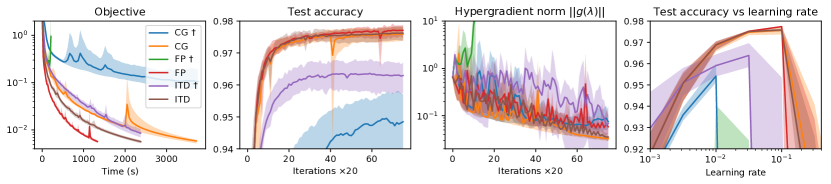
Figure 3: Experiments with convolutional EQMs. Mean (solid line) and point-wise minimum-maximum range (shaded region) across 5 random seeds. The seed only controls the initialization of $\lambda$. The estimated hypergradient $g(\lambda)$ is equal to $\nabla f_{t}(\lambda)$ for ITD and $\hat{\nabla}f(\lambda)$ for AID. We used $t=k=20$ for all methods and Nesterov momentum (1500 iterations) for optimizing $\lambda$, applying a projector operator at each iteration except for the methods marked with ${\dagger}$. Note that in the first three plots the step-size for the unconstrained experiments is smaller, to prevent divergence.

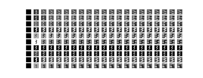
Figure 4: Images of two samples of the states filter maps $w_{i}\in\mathbb{R}^{10\times 14\times 14}$ for a three and a six from the MNIST dataset, learnt with the fixed-point method and with projection. Each of the ten rows represents a filter and the x-axis proceeds with the iterations of the EQM dynamics (for a total of $t=20$ iterations). The states are initialized to $0$ (black images on the left) and then the mapping (37) is iterated 20 times to approximately reach the fixed point representation (rightmost images).

In this section we report a series of experiments on equilibrium models quite similar to those of the last paragraph of Section 3.2, but with convolutional and max-pooling operators in place of the affinities of Equation (23). In particular we model the learnable dynamics with parameters $\gamma=(K,K^{\prime},c)$ as

$$\phi_{i}(w_{i},\gamma)=\tanh{\left(K\star w_{i}+\mu_{2\times 2}(K^{\prime}\star x_{i})+c\right)}$$ (37)

where $w_{i}\in\mathbb{R}^{h\times 14\times 14}$ are the state feature maps, $\star$ denotes multi-channel bidimensional cross-correlation, $K$ and $K^{\prime}$ contain $h$ $3\times 3$ convolutional kernels each and $\mu_{2\times 2}$ denotes the max-pooling operator with a $2\times 2$ field and stride of $2$. The state feature maps are passed through a max-pooling operator before being flattened and fed to a multiclass logistic classifier. We set $h=10$ for all the experiments. We use the results and the code of Sedghi et al. (2019) to efficiently perform the projection of the linear operator associated to $K$ into the unit spectral ball. Data and optimization method for the upper objective are the same of Section 3.2.

The results, reported in Figure 3, show similar behaviours of those in Section 3.2, albeit with more marked differences among the methods, especially for the experiments without projection (denoted by ${\dagger}$ in the figure). The statistical performances of the contractive convolutional EQM exceed abundantly those given by simpler dynamics of (23), with the fixed-point method (red line) being slightly better then the others. We show some visual examples of the learned dynamics in Figure 4, where we plot the 10 bidimensional state filter maps as the iterations of (37) proceed.

Interestingly, when the projection is not performed, optimization with the fixed-point scheme to compute the hypergradient (akin to recurrent backpropagation, see green shaded region in the rightmost plot of Figure 3) does not reliably converge for all the probed values of the step-size, indicating once more the importance of the contractiveness assumption for AID methods. We finally note that regularizing the norm of $\partial_{1}\phi_{i}$ or adding $L_{1}$ or $L_{\infty}$ penalty terms on the matrix of the state-wise linear transformation may encourage, but does not strictly enforce, such condition. This may in part explain some difficulties previously encountered in training EQM-like models, e.g. in the context of relational learning (graph neural networks).

References

• Almeida (1987) Almeida, L. B. A learning rule for asynchronous perceptrons with feedback in a combinatorial environment. In Proceedings, 1st First International Conference on Neural Networks, volume 2, pp.  609–618, 1987.
• Amos (2019) Amos, B. Differentiable optimization-based modeling for machine learning. PhD thesis, PhD thesis. Carnegie Mellon University, 2019.
• Amos & Kolter (2017) Amos, B. and Kolter, J. Z. Optnet: Differentiable optimization as a layer in neural networks. In Proceedings of the 34th International Conference on Machine Learning-Volume 70, pp.  136–145, 2017.
• Andrychowicz et al. (2016) Andrychowicz, M., Denil, M., Gomez, S., Hoffman, M. W., Pfau, D., Schaul, T., Shillingford, B., and De Freitas, N. Learning to learn by gradient descent by gradient descent. In Advances in neural information processing systems, pp. 3981–3989, 2016.
• Bai et al. (2019) Bai, S., Kolter, J. Z., and Koltun, V. Deep equilibrium models. In Advances in Neural Information Processing Systems, pp. 688–699, 2019.
• Baydin et al. (2018) Baydin, A. G., Pearlmutter, B. A., Radul, A. A., and Siskind, J. M. Automatic differentiation in machine learning: a survey. Journal of Machine Learning Research, 18(153), 2018.
• Bergstra & Bengio (2012) Bergstra, J. and Bengio, Y. Random search for hyper-parameter optimization. Journal of Machine Learning Research, 13(Feb):281–305, 2012.
• Bertinetto et al. (2019) Bertinetto, L., Henriques, J. F., Torr, P. H., and Vedaldi, A. Meta-learning with differentiable closed-form solvers. ICLR, 2019.
• Denevi et al. (2019) Denevi, G., Ciliberto, C., Grazzi, R., and Pontil, M. Learning-to-learn stochastic gradient descent with biased regularization. In Proc. 36th International Conference on Machine Learning, volume 97 of PMLR, pp.  1566–1575, 2019.
• Domke (2012) Domke, J. Generic methods for optimization-based modeling. In Artificial Intelligence and Statistics, pp.  318–326, 2012.
• Elsken et al. (2019) Elsken, T., Metzen, J. H., and Hutter, F. Neural architecture search: A survey. Journal of Machine Learning Research, 20(55):1–21, 2019.
• Finn et al. (2017) Finn, C., Abbeel, P., and Levine, S. Model-agnostic meta-learning for fast adaptation of deep networks. In Proceedings of the 34th International Conference on Machine Learning-Volume 70, pp.  1126–1135, 2017.
• Franceschi et al. (2017) Franceschi, L., Donini, M., Frasconi, P., and Pontil, M. Forward and reverse gradient-based hyperparameter optimization. In Proceedings of the 34th International Conference on Machine Learning-Volume 70, pp.  1165–1173, 2017.
• Franceschi et al. (2018) Franceschi, L., Frasconi, P., Salzo, S., Grazzi, R., and Pontil, M. Bilevel programming for hyperparameter optimization and meta-learning. In International Conference on Machine Learning, pp. 1563–1572, 2018.
• Griewank & Walther (2008) Griewank, A. and Walther, A. Evaluating Derivatives: Principles and Techniques of Algorithmic Differentiation, volume 105. Siam, 2008.
• Liao et al. (2018) Liao, R., Xiong, Y., Fetaya, E., Zhang, L., Yoon, K., Pitkow, X., Urtasun, R., and Zemel, R. Reviving and improving recurrent back-propagation. In International Conference on Machine Learning, pp. 3088–3097, 2018.
• Little et al. (2008) Little, M., McSharry, P., Hunter, E., Spielman, J., and Ramig, L. Suitability of dysphonia measurements for telemonitoring of parkinson’s disease. Nature Precedings, pp.  1–1, 2008.
• Liu et al. (2018) Liu, H., Simonyan, K., and Yang, Y. Darts: Differentiable architecture search. arXiv preprint arXiv:1806.09055, 2018.
• Lorraine et al. (2019) Lorraine, J., Vicol, P., and Duvenaud, D. Optimizing millions of hyperparameters by implicit differentiation. arXiv preprint arXiv:1911.02590, 2019.
• Maclaurin et al. (2015) Maclaurin, D., Duvenaud, D., and Adams, R. Gradient-based hyperparameter optimization through reversible learning. In International Conference on Machine Learning, pp. 2113–2122, 2015.
• Mehra & Hamm (2019) Mehra, A. and Hamm, J. Penalty method for inversion-free deep bilevel optimization. arXiv preprint arXiv:1911.03432, 2019.
• Miller & Hardt (2019) Miller, J. and Hardt, M. Stable recurrent models. ICLR, 2019.
• Nesterov (1983) Nesterov, Y. E. A method for solving the convex programming problem with convergence rate o (1/k^ 2). In Dokl. akad. nauk Sssr, volume 269, pp.  543–547, 1983.
• Paszke et al. (2019) Paszke, A., Gross, S., Massa, F., Lerer, A., Bradbury, J., Chanan, G., Killeen, T., Lin, Z., Gimelshein, N., Antiga, L., Desmaison, A., Kopf, A., Yang, E., DeVito, Z., Raison, M., Tejani, A., Chilamkurthy, S., Steiner, B., Fang, L., Bai, J., and Chintala, S. Pytorch: An imperative style, high-performance deep learning library. In Advances in Neural Information Processing Systems 32, pp. 8024–8035. 2019.
• Pedregosa (2016) Pedregosa, F. Hyperparameter optimization with approximate gradient. In International Conference on Machine Learning, pp. 737–746, 2016.
• Pineda (1987) Pineda, F. J. Generalization of back-propagation to recurrent neural networks. Physical review letters, 59(19):2229, 1987.
• Polyak (1987) Polyak, B. T. Introduction to Optimization. Optimization Software Inc. Publication Division, New York, NY, USA, 1987.
• Rajeswaran et al. (2019) Rajeswaran, A., Finn, C., Kakade, S. M., and Levine, S. Meta-learning with implicit gradients. In Advances in Neural Information Processing Systems, pp. 113–124, 2019.
• Scarselli et al. (2008) Scarselli, F., Gori, M., Tsoi, A. C., Hagenbuchner, M., and Monfardini, G. The graph neural network model. IEEE Transactions on Neural Networks, 20(1):61–80, 2008.
• Sedghi et al. (2019) Sedghi, H., Gupta, V., and Long, P. M. The singular values of convolutional layers. ICLR, 2019.
• Shaban et al. (2019) Shaban, A., Cheng, C.-A., Hatch, N., and Boots, B. Truncated back-propagation for bilevel optimization. In The 22nd International Conference on Artificial Intelligence and Statistics, pp.  1723–1732, 2019.
• Snoek et al. (2012) Snoek, J., Larochelle, H., and Adams, R. P. Practical bayesian optimization of machine learning algorithms. In Advances in neural information processing systems, pp. 2951–2959, 2012.
• Xiao et al. (2017) Xiao, H., Rasul, K., and Vollgraf, R. Fashion-mnist: a novel image dataset for benchmarking machine learning algorithms, 2017.