Partitioned Least Squares

Abstract

In this paper we propose a variant of the linear least squares model allowing practitioners to partition the input features into groups of variables that they require to contribute similarly to the final result. The output allows practitioners to assess the importance of each group and of each variable in the group. We formally show that the new formulation is not convex and provide two alternative methods to deal with the problem: one non-exact method based on an alternating least squares approach; and one exact method based on a reformulation of the problem using an exponential number of sub-problems whose minimum is guaranteed to be the optimal solution. We formally show the correctness of the exact method and also compare the two solutions showing that the exact solution provides better results in a fraction of the time required by the alternating least squares solution (assuming that the number of partitions is small). For the sake of completeness, we also provide an alternative branch and bound algorithm that can be used in place of the exact method when the number of partitions is too large, and a proof of NP-completeness of the optimization problem introduced in this paper.

1 Introduction

Linear regression models are among the most extensively employed statistical methods in science and industry alike (Bro et al., 2002; Intriligator et al., 1978; Isobe et al., 1990; Nievergelt, 2000; Reeder et al., 2004). Their simplicity, ease of use and performance in low-data regimes enables their usage in various prediction tasks. As the number of observations usually exceeds the number of variables, a practitioner has to resort to approximating the solution of an overdetermined system. Least squares approximation benefits from a closed-form solution and is the oldest (Gauss, 1995) and most known approach in linear regression analysis. Among the benefits of linear regression models there is the possibility of easily interpreting how much each variate is contributing to the approximation of the dependent variable by means of observing the magnitudes and signs of the associated parameters.

In some application domains, partitioning the variables in non-overlapping subsets is beneficial either as a way to insert human knowledge into the regression analysis task or to further improve model interpretability. When considering high-dimensionality data, grouping variables together is also a natural way to make it easier to reason about the data and the regression result. As an example, consider a regression task where the dependent variable is the score achieved by students in an University or College exam. A natural way to group the dependent variables is to divide them into two groups where one contains the variables which represent a student’s effort in the specific exam (hours spent studying, number of lectures attended…), while another contains the variables related to previous effort and background (number of previous exams passed, number of years spent at University or College, grade average…). Assuming all these variables could be measured accurately, it might be interesting to know how much each group of variables contributes to the student’s score. As a further example, when analyzing complex chemical compounds, it is possible to group together fine-grained features to obtain a partition which refers to high-level properties of the compound (such as structural, interactive and bond-forming among others), and knowing how much each high-level property contributes to the result of the analysis is often of great practical value (Caron et al., 2013).

In this paper we introduce a variation on the linear regression problem which allows for partitioning variables into meaningful groups. The parameters obtained by solving the problem allow one to easily assess the contribution of each group to the dependent variable as well as the importance of each element of the group.

The newly introduced problem is not easy to solve and indeed we will prove the non-convexity of the objective, and the NP-completeness of the problem itself. In Section 3 we introduce two possible algorithms to solve the problem. One is based on an Alternate Convex Search method (Wendell and Hurter Jr., 1976), where the optimization of the parameters is iterative and can get trapped into local minima; the other is based on a reformulation of the original problem into an exponential number of sub-problems, where the exponent is the cardinality $K$ of the partition. We prove convergence of the alternating least square algorithm and the global optimality of the result returned by the second approach. We also provide guidance for building a branch and bound (Lawler and Wood, 1966) solution that might be useful when the cardinality of the partition is too large to use the exact algorithm.

We test the two algorithms on several datasets. Our experiments include data extracted from the analysis of chemical compounds (Caron et al., 2013) in a particular setting where this kind of analysis already proved to be of value to practitioners, and a number of datasets having a large amount of features which we selected from the UCI repository (Dua and Graff, 2017): in this latter case the number, size, and composition of the partition has been decided arbitrarily just to experiment with the provided algorithms. Our experimental results show that the exact algorithm is usually a good choice, the non-exact algorithm being preferable when high accuracy is not required and/or the cardinality of the partition is too large.

While to the best of our knowledge the regression problem and the algorithms we present are novel, there has been previous work dealing with alternative formulations to the linear regression problem. Some of them have shown to be of great practical use and have received attention from both researchers and practitioners.

Partial Least Squares (PLS) Regression (Wold et al., 2001) is a very popular method in hard sciences such as chemists and chemometrics. PLS has been designed to address the bad behavior of ordinary least squares when the dataset is small, especially when the number of features is large in comparison. In such cases, one can try to select a smaller set of features allowing a better behavior. A very popular way to select important features is to use Principal Component Analysis (PCA) to select the features that contributes most to the variation in the dataset. However, since PCA is based on the data matrix alone, one risks to filter out features that are highly correlated with the target variables in $\mathbf{Y}$. PLS has been explicitly designed to solve this problem by decomposing $\mathbf{X}$ and $\mathbf{Y}$ simultaneously and in such a way to explain as much as possible of the covariance between $\mathbf{X}$ and $\mathbf{Y}$ (Abdi, 2010). Our work is substantially different from these approaches since we are not concerned at all with the goal of removing variables. On the contrary, we group them so to make the result more interpretable and to provide valuable information about the importance of each group.

Yet another set of techniques that resembles our work are those where a partition of the variables is used to select groups of features. Very well known members of this family of algorithms are group lasso methods (Bakin, 1999; Yuan and Lin, 2006) (Huang et al. (2012) provide a review of such methodologies). In these works, the authors tackle the problem of selecting grouped variables for accurate prediction. In this case, as in ours, the groups for the variables are defined by the user, but in their case the algorithm needs to predict which subset of the groups will lead to better performances (i.e., either all variables in a group will be used as part of the solution or none of them will be). This is a rather different problem with respect to the one that we introduce here. In our case, we shall assume that all groups are relevant to the analysis. However, in our case we seek a solution where all variables in the same group contributes in the same direction (i.e., with the same sign) to the solution. We argue that this formulation allows for an easier interpretation of the contribution of the whole group as well as of the variables included in each group.

In this paper we introduce a new least squares problem and provide algorithms to solve it. Our contributions include:

• The definition of the Partitioned Least Squares (PartitionedLS) problem;

• A formal non-convexity proof for the objective of the PartitionedLS problem;

• PartLS-alt: an iterative algorithm solving the PartitionedLS problem;

• PartLS-opt: an optimal algorithm solving the PartitionedLS problem;

• A formal proof of convergence of PartLS-alt;

• A formal proof of the global optimality of PartLS-opt;

• The main ideas needed to implement a branch and bound solution aimed at optimizing PartLS-opt;

• A formal proof of NP-completeness of the PartitionedLS problem;

• Information about how to update the algorithms to regularize the solutions;

• Information about how to leverage the non-negative least squares algorithm (Lawson and Hanson, 1995) to improve numerical stability;

• An experimentation of the two algorithms over several datasets.

2 Model description

Table 1: Notation

Symbol(s)	Definition
$a_{i}$	$i$-th component of vector ${\boldsymbol{a}}$.
$(\cdot)_{n}$	Shorthand to specify vectors (or matrices) in terms of their components. For instance $(i)_{i}$ shall denote a vector ${\boldsymbol{v}}$ such that $v_{i}=i$.
$k$, $K$	$k$ is the index for iterating over the $K$ subsets belonging to the partition.
$m$, $M$	$m$ is the index for iterating over the $M$ variables.
$\mathbf{X}$	an $N\times M$ matrix containing the descriptions of the training instances.
$\mathbf{A}\times\mathbf{B}$	matrix multiplication operation (we also simply write it $\mathbf{A}\mathbf{B}$ when the notation appears clearer).
${\boldsymbol{y}}$	a vector of length $N$ containing the labels assigned to the examples in $\mathbf{X}$.
$\bullet$	wildcard used in subscriptions to denote whole columns or whole rows: e.g., ${\boldsymbol{X}}_{\bullet,k}$ denotes the $k$-th column of matrix $\mathbf{X}$ and ${\boldsymbol{X}}_{m,\bullet}$ denotes its $m$-th row.
$\star$	denotes an optimal solution, e.g., $p^{\star}$ denotes the optimal solution of the PartitionedLS problem, while $p_{b}^{\star}$ denotes the optimal solution of the PartitionedLS-b problem.
$\mathbf{P}$	a $M\times K$ partition matrix, $P_{m,k}\in\{0,1\}$, with $P_{m,k}=1$ iff variable $\alpha_{m}$ belongs to the $k$-th element of the partition.
$P_{k}$	the set of all indices in the $k$-th element of the partition: $\{m|P_{k,m}=1\}$.
$k[m]$	index of the partition element to which $\alpha_{m}$ belongs, i.e.: $k[m]$ is such that $m\in P_{k[m]}$.
$\circ$	Hadamard (i.e., element-wise) product. When used to multiply a matrix by a column vector, it is intended that the columns of the matrix are each one multiplied (element-wise) by the column vector.
$\oslash$	Hadamard (i.e., element-wise) division.
$\succeq$	element-wise larger-than operator: ${\boldsymbol{\alpha}}\succeq 0$ is equivalent to $\alpha_{m}\geq 0$ for $m\in{1..M}$.

In this work we denote matrices with capital bold letters such as $\mathbf{X}$ and vectors with lowercase bold letters as ${\boldsymbol{v}}$. In the text we use a regular (non-bold) font weight when we refer to the name of the vector or when we refer to scalar values contained in the vector. In other words, we use the bold face only when we refer to the vector itself. For instance, we might say that the values in the $\alpha$ vector are those contained in the vector ${\boldsymbol{\alpha}}$, which contains in position $i$ the scalar $\alpha_{i}$. We consistently define each piece of notation as soon as we use it, but we also report it in Table 1, where the reader can more easily access the whole notation employed throughout the paper.

Let us consider the problem of inferring a linear least squares model to predict a real variable $y$ given a vector ${\boldsymbol{x}}\in\mathbb{R}^{M}$. We will assume that the examples are available at learning time as an $N\times M$ matrix $\mathbf{X}$ and $N\times 1$ column vector ${\boldsymbol{y}}$. We will also assume that the problem is expressed in homogeneous coordinates, i.e., that $\mathbf{X}$ has an additional column containing values equal to $1$, and that the intercept term of the affine function is included into the weight vector ${\boldsymbol{w}}$ to be computed.

The standard least squares formulation for the problem at hand is to minimize the quadratic loss over the residuals, i.e.:

$$\text{minimize}_{{\boldsymbol{w}}}\|\mathbf{X}{\boldsymbol{w}}-{\boldsymbol{y}}\|_{2}^{2}.$$

This is a problem that has the closed form solution ${\boldsymbol{w}}=(\mathbf{X}^{T}\mathbf{X})^{-1}\mathbf{X}^{T}{\boldsymbol{y}}$. As mentioned in Section 1, in many application contexts where $M$ is large, the resulting model is hard to interpret. However, it is often the case that domain experts can partition the elements in the weights vector into a small number of groups and that a model built on this partition would be much easier to interpret. Then, let $\mathbf{P}$ be a “partition” matrix for the problem at hand (this is not a partition matrix in the linear algebra sense, it is simply a matrix containing the information needed to partition the features of the problem). More formally, let $\mathbf{P}$ be a $M\times K$ matrix where $P_{m,k}\in\{0,1\}$ is equal to $1$ iff feature number $m$ belongs to the $k$-th partition element. We will also write $P_{k}$ to denote the set $\{m|P_{m,k}=1\}$ of all the features belonging to the $k$-th partition element.

Here we introduce the Partitioned Least Squares (PartitionedLS) problem, a model where we introduce $K$ additional variables and express the whole regression problem in terms of these new variables (and in terms of how the original variables contribute to the predictions made using them). The simplest way to describe the new model is to consider its regression function (to make the discussion easier, we start with the data matrix $\mathbf{X}$ expressed in non-homogenous coordinates and switch to homogenous coordinates afterwards):

$$f(\mathbf{X})=\left(\sum_{k=1}^{K}\beta_{k}\sum_{m\in P_{k}}\alpha_{m}x_{n,m}+t\right)_{n},$$ (1)

i.e., $f({\bf X})$ computes a vector whose $n$-th component is the one reported within parenthesis (see Table 1 for details on the notation). The first summation is over the $K$ sets in the partition that domain experts have identified as relevant, while the second one iterates over all variables in that set. We note that the $m$-th $\alpha$ weight contributes to the $k$-th element of the partition only if feature number $m$ belongs to it. As we shall see, we require that all $\alpha$ values are nonnegative, and that $\forall k:\sum_{m\in P_{k}}\alpha_{m}=1$. Consequently, the expression returns a vector of predictions calculated in terms of two sets of weights: the $\beta$ weights, which are meant to capture the magnitude and the sign of the contribution of the $k$-th element of the partition, and the $\alpha$ weights, which are meant to capture how each feature in the $k$-th set contributes to it. We note that the $\alpha$ weight vector is of the same length as the vector ${\boldsymbol{w}}$ in the least squares formulation. Despite this similarity, we prefer to use a different symbol because the interpretation of (and the constraints on) the $\alpha$ weights are different with respect to the $w$ weights.

It is easy to verify that the definition of $f$ in (1) can be rewritten in matrix notation as:

$$f(\mathbf{X})=\left(\sum_{k=1}^{K}\beta_{k}\sum_{m}P_{m,k}\alpha_{m}x_{n,m}+t\right)_{n}=\mathbf{X}\times(\mathbf{P}\circ{\boldsymbol{\alpha}})\times{\boldsymbol{\beta}}+t,$$ (2)

where $\circ$ is the Hadamard product extended to handle column-wise products. More formally, if $\mathbf{Z}$ is a $A\times B$ matrix, ${\boldsymbol{1}}$ is a $B$ dimensional vector with all entries equal to $1$, and ${\boldsymbol{a}}$ is a column vector of length $A$, then $\mathbf{Z}\circ{\boldsymbol{a}}\triangleq\mathbf{Z}\circ({\boldsymbol{a}}\times\mathbf{1}^{T})$; where the $\circ$ symbol on the right hand side of the definition is the standard Hadamard product. Equation (2) can be rewritten in homogeneous coordinates as:

$$f(\mathbf{X})=\mathbf{X}\times(\mathbf{P}\circ{\boldsymbol{\alpha}})\times{\boldsymbol{\beta}},$$ (3)

where $\mathbf{X}$ incorporates a column with all entries equal to 1, and we consider an additional group (with index $K+1$) having a single $\alpha_{M+1}$ variable in it. Given the constraints on $\alpha$ variables, $\alpha_{M+1}$ is forced to assume a value equal to $1$ and the value of $t$ is then totally incorporated into $\beta_{K+1}$. In the following we will assume for ease of notation that the problem is given in homogeneous coordinates and that the constants $M$ and $K$ already account for the additional single-variable group.

Definition 1

The partitioned least square (PartitionedLS) problem is formulated as:

$$\text{minimize}_{{\boldsymbol{\alpha}},{\boldsymbol{\beta}}}\|\mathbf{X}\times(\mathbf{P}\circ{\boldsymbol{\alpha}})\times{\boldsymbol{\beta}}-{\boldsymbol{y}}\|_{2}^{2}$$

$$\begin{aligned} \textup{s.t.}\quad&{\boldsymbol{\alpha}}\succeq 0\\ &\mathbf{\mathbf{P}}^{T}\times{\boldsymbol{\alpha}}={\boldsymbol{1}}.\end{aligned}$$

In summary, we want to minimize the squared residuals of $f(\mathbf{X})$, as defined in (3), under the constraint that for each subset $k$ in the partition, the set of weights form a distribution: they need to be all nonnegative as imposed by ${\boldsymbol{\alpha}}\succeq 0$ constraint and they need to sum to $1$ as imposed by constraint $\mathbf{\mathbf{P}}^{T}\times{\boldsymbol{\alpha}}={\boldsymbol{1}}$.

Unfortunately we do not know a closed form solution for this problem. Furthermore, the problem is not convex and hence hard to solve to global optimality using standard out-of-the-box solvers. Even worse, later on we shall prove that the problem is actually NP-complete. The following theorem states the non-convexity of the objective function formally.

Theorem 1

The PartitionedLS problem is not convex.

Proof 1

It suffices to show that the Hessian of the objective function is not positive semidefinite. By Schwarz’s theorem, since the loss function has continuous second partial derivatives, the matrix is symmetric and we can apply the Sylvester criterion for checking positive definiteness. In practice, we prove that the Hessian is not positive semidefinite by showing that not all leading principal minors are larger than zero. In our specific case, the second minor can be shown to assume values smaller than zero and this proves the theorem. In summary, we need to show that the second principal minor can be smaller than zero, in formulae:

$$\left|\begin{array}[]{cc}H_{11}&H_{12}\\ H_{21}&H_{22}\end{array}\right|=H_{11}H_{22}-H_{12}H_{21}<0.$$

Let us denote with $L$ the objective of the PartitionedLS problem

$$L =\|\mathbf{X}\times(\mathbf{P}\circ{\boldsymbol{\alpha}})\times{\boldsymbol{\beta}}-{\boldsymbol{y}}\|^{2}_{2}$$

$$=\sum_{n}\left(\sum_{k}\beta_{k}\sum_{\alpha_{m}\in P_{k}}\alpha_{m}x_{n,m}-y_{n}\right)^{2}.$$

In evaluating the derivatives, we consider the variables of the PartitionedLS problem in the following order: $(\alpha_{1},\beta_{1},\alpha_{2},\beta_{2},\dots,\alpha_{K},\beta_{K},\alpha_{K+1},\alpha_{K+2},\dots,\alpha_{M})$ and assume the problem is not trivial, i.e., that $m>1,k>1$. In the following, without loss of generality, we will assume that $\alpha_{1}\in P_{1}$. Under these assumptions, to prove that the second minor is smaller than zero amounts to prove that:

$$H_{11}H_{22}-H_{12}H_{21} =\frac{\partial^{2}L}{\partial\alpha_{1}\partial\alpha_{1}}\frac{\partial^{2}L}{\partial\beta_{1}\partial\beta_{1}}-\frac{\partial^{2}L}{\partial\alpha_{1}\partial\beta_{1}}\frac{\partial^{2}L}{\partial\beta_{1}\partial\alpha_{1}}$$

$$=\frac{\partial^{2}L}{\partial\alpha_{1}^{2}}\frac{\partial^{2}L}{\partial\beta_{1}^{2}}-\left(\frac{\partial^{2}L}{\partial\alpha_{1}\partial\beta_{1}}\right)^{2}<0.$$

The partial derivative of the loss function with respect to a specific variable $\alpha_{\overline{m}}$ is:

$$\frac{\partial L}{\partial\alpha_{\overline{m}}} =\sum_{n}2\left(\sum_{k}\beta_{k}\sum_{m\in P_{k}}\alpha_{m}x_{n,m}-y_{n}\right)\beta_{k[\overline{m}]}x_{n,\overline{m}}$$

$$=2\sum_{n}\rho_{\alpha,\beta}(n)\beta_{k[\overline{m}]}x_{n,\overline{m}}$$

$$=2\beta_{k[\overline{m}]}\sum_{n}\rho_{\alpha,\beta}(n)x_{n,\overline{m}},$$

where $k[\overline{m}]$ denotes the index of the partition to which feature $\overline{m}$ belongs and, for the sake of convenience, we define:

$$\rho_{\alpha,\beta}(n)=\sum_{k}\beta_{k}\sum_{m\in P_{k}}\alpha_{m}x_{n,m}-y_{n}.$$

The partial derivative w.r.t. one of the $\beta$ variables is:

$$\frac{\partial L}{\partial\beta_{k}}=2\sum_{n}\rho_{\alpha,\beta}(n)\sum_{m\in P_{k}}\alpha_{m}x_{n,m}.$$

The second order derivatives we are interested into are:

$$\frac{\partial^{2}L}{\partial\alpha_{m}^{2}} =2\beta_{k[m]}\sum_{n}x_{n,m}\frac{\partial}{\partial\alpha_{m}}\rho_{\alpha,\beta}(n)=2\beta_{k[m]}\sum_{n}x_{n,m}\beta_{k[m]}x_{n,m}$$

$$=2\beta^{2}_{k[m]}\sum_{n}x^{2}_{n,m}$$

$$\frac{\partial^{2}L}{\partial\beta_{k}^{2}} =2\sum_{n}\left(\sum_{m\in P_{k}}\alpha_{m}x_{n,m}\right)^{2}$$

$$\frac{\partial^{2}L}{\partial\alpha_{m}\partial\beta_{k}} =2\sum_{n}\frac{\partial}{\partial\beta_{k}}\left[\beta_{k}x_{n,m}\rho_{\alpha,\beta}(n)\right]$$

$$=2\sum_{n}\left[x_{n,m}\rho_{\alpha,\beta}(n)+\beta_{k}x_{n,m}\sum_{\overline{m}\in P_{k}}\alpha_{\overline{m}}x_{n,\overline{m}}\right],$$

where we assumed $k[m]=k$ since in the case we are interested, we have $m=1,k=1$ and $\alpha_{1}\in P_{1}$. Instantiating these derivatives for $k=1,m=1$:

$$H_{11}H_{22}-H_{12}H_{21}= \left(2\beta^{2}_{1}\sum_{n}x^{2}_{n,1}\right)2\sum_{n}\left(\sum_{m\in P_{1}}\alpha_{\overline{m}}x_{n,m}\right)^{2}$$

$$-\left[2\sum_{n}x_{n,1}\left(\beta_{1}\sum_{m\in P_{1}}\alpha_{m}x_{n,m}+\rho_{\alpha,\beta}(n)\right)\right]^{2}.$$ (4)

Now, it is enough to observe that the term on the left hand-side of the minus sign only depends on $\beta_{1}$, while the term on the right-hand side of the minus sign depends also on $\beta_{2},\ldots,\beta_{K}$ and can be made arbitrarily large as we increase the values of these variables, thus making (1) negative and the Hessian not semidefinite positive.

In the following we will provide two algorithms that solve the above problem. One is an alternating least squares approach which scales well with $K$, but it is not guaranteed to provide the globally optimal solution. The other one is a reformulation of the problem through a (possibly) large number of convex problems whose minimum is guaranteed to be the globally optimal solution of the original problem. Even though the second algorithm does not scale well with $K$, we believe that this should not be a problem since the PartitionedLS is by design well suited for a small group of interpretable groups. However, we do sketch a possible branch and bound strategy to mitigate this problem in Section 3.4.

Remark 1

The PartitionedLS model presented so far has no regularization mechanism in place and, as such, it risks overfitting the training set. Since the $\alpha$ values are normalized by definition, the only parameters that need regularization are those collected in the ${\boldsymbol{\beta}}$ vector. Then, the regularized version of the objective function simply adds a penalty on the size of the ${\boldsymbol{\beta}}$ vector:

$$\|\mathbf{X}\times(\mathbf{P}\circ{\boldsymbol{\alpha}})\times{\boldsymbol{\beta}}\|^{2}_{2}+\eta\|{\boldsymbol{\beta}}\|^{2}_{2},$$ (5)

where the squared euclidean norm could be substituted with the L1 norm in case a LASSO-like regularization is preferred.

3 Algorithms

3.1 Alternating Least Squares approach

In the PartitionedLS problem we aim at minimizing a non-convex objective, where the non-convexity depends on the multiplicative interaction between $\alpha$ and $\beta$ variables in the expression $\|\mathbf{X}\times(\mathbf{P}\circ{\boldsymbol{\alpha}})\times{\boldsymbol{\beta}}-{\boldsymbol{y}}\|_{2}^{2}$. Interestingly, if one fixes ${\boldsymbol{\alpha}}$, the expression $\mathbf{X}\times(\mathbf{P}\circ{\boldsymbol{\alpha}})$ results in a matrix $\mathbf{X}^{\prime}$ that does not depend on any variable. Then, the whole expression can be rewritten as a problem $p_{\boldsymbol{\alpha}}$ whose objective function $\|\mathbf{X}^{\prime}{\boldsymbol{\beta}}-{\boldsymbol{y}}\|_{2}^{2}$ depends on the parameter vector ${\boldsymbol{\alpha}}$ and is the convex objective function of a standard least squares problem in the $\beta$ variables. In a similar way, it can be shown that by fixing ${\boldsymbol{\beta}}$ one also ends up with a convex optimization problem $p_{\boldsymbol{\beta}}$. Indeed, after fixing ${\boldsymbol{\beta}}$, the objective function is the squared norm of a vector whose components are affine functions of vector ${\boldsymbol{\alpha}}$ (see Section 3.3 for more details). These observations naturally lead to the formulation of an alternating least squares solution where one alternates between solving $p_{\boldsymbol{\alpha}}$ and $p_{\boldsymbol{\beta}}$. In Algorithm 1 we formalize this intuition into the PartLS-alt function where, after initializing ${\boldsymbol{\alpha}}$ and ${\boldsymbol{\beta}}$ randomly, we iterate until some stopping criterion is satisfied (in our experiments we fixed a number $T$ of iterations, but one may want to stop the algorithm as soon as ${\boldsymbol{a}}$ and ${\boldsymbol{c}}$ do not change between two iterations). At each iteration we take the latest estimate for the $\alpha$ variables and solve the $p_{\boldsymbol{\alpha}}$ problem based on that estimate, we then keep the newly found $\beta$ variables and solve the $p_{\boldsymbol{\beta}}$ problem based on them. At each iteration the overall objective is guaranteed not to increase in value and, indeed, we prove that, if the algorithm is never stopped, the sequence of ${\boldsymbol{\alpha}}$ and ${\boldsymbol{\beta}}$ vectors found by PartLS-alt has at least one accumulation point and that all accumulation points are partial optima with the same function value.

Theorem 2

Let ${\boldsymbol{\zeta}}_{i}=({\boldsymbol{\alpha}}_{i},{\boldsymbol{\beta}}_{i})$ be the sequence of ${\boldsymbol{\alpha}}$ and ${\boldsymbol{\beta}}$ vectors found by PartLS-alt to the PartitionedLS problem and assume that the objective function is regularized as described in (5), then:

1. the sequence of ${\boldsymbol{\zeta}}_{i}$ has at least one accumulation point, and

2. all accumulation points are partial optima attaining the same value of the objective function.

Proof 2

The PartitionedLS problem is actually a biconvex optimization problem and Algorithm 1 is actually a specific instantiation of the Alternating Convex Search strategy (Gorski et al., 2007) to solve biconvex problems. Theorem 4.9 in (Gorski et al., 2007) implies that:

• if the sequence ${\boldsymbol{\zeta}}_{i}$ is contained in a compact set then it has at least one accumulation point, and

• if for each accumulation point ${\boldsymbol{\zeta}}^{\star}$ of the sequence ${\boldsymbol{\zeta}}_{i}$, either the optimal solution of the problem with fixed ${\boldsymbol{\alpha}}$ is unique, or the optimal solution of the problem with fixed ${\boldsymbol{\beta}}$ is unique; then all accumulation points are partial optima and have the same function value.

The first requirement is fulfilled in our case since ${\boldsymbol{\alpha}}$ is constrained by definition into $[0,1]^{M}$, while the regularization term prevents ${\boldsymbol{\beta}}$ from growing indefinitely. The second requirement is fulfilled since for fixed ${\boldsymbol{\alpha}}$ the optimization function is quadratic and strictly convex in ${\boldsymbol{\beta}}$. Hence, the solution is unique.

Algorithm 1: Alternating least squares solution to the PartitionedLS problem. The notation $\mathtt{const}$(${\boldsymbol{\alpha}}$) (respectively $\mathtt{const}$(${\boldsymbol{\beta}}$)) is just to emphasize that the current value of ${\boldsymbol{\alpha}}$ (respectively ${\boldsymbol{\beta}}$) will be used as a constant in the following step.

⬇

1 function PartLS-alt($\mathbf{X},{\boldsymbol{y}},\mathbf{P}$)

2 ${\boldsymbol{\alpha}}$ = random(M)

3 ${\boldsymbol{\beta}}$ = random(K)

4

5 for $t$ in $1\dots T$

6 ${\boldsymbol{a}}$ = const(${\boldsymbol{\alpha}}$)

7 $p^{\star}$ = minimize_β($\|(\mathbf{X}\times(\mathbf{P}\circ{\boldsymbol{a}})\times{\boldsymbol{\beta}}-{\boldsymbol{y}}\|_{2}^{2})$)

8

9

10 ${\boldsymbol{c}}$ = const(${\boldsymbol{\beta}}$)

11 $p^{\star}$ = minimize_α($\|(\mathbf{X}\times(\mathbf{P}\circ{\boldsymbol{\alpha}})\times{\boldsymbol{c}}-{\boldsymbol{y}}\|_{2}^{2}$,

12 ${\boldsymbol{\alpha}}\succeq 0$,

13 $\mathbf{\mathbf{P}}^{T}\times{\boldsymbol{\alpha}}=1$)

14 end

15

16 return $(p^{\star},{\boldsymbol{\alpha}},{\boldsymbol{\beta}})$

17 end

3.2 Reformulation as a set of convex subproblems

Here we show how the PartitionedLS problem can be reformulated as a new problem with binary variables which, in turn, can be split into a set of convex problems such that the smallest objective function value among all local (and global) minimizers of these convex problems is also the global optimum value of the PartitionedLS problem.

Definition 2

The PartitionedLS-b problem is a PartitionedLS problem in which the $\beta$ variables are substituted by a binary variable vector ${\boldsymbol{b}}\in\{-1,1\}^{K}$, and the normalization constraints over the $\alpha$ variables are dropped:

$$\text{minimize}_{{\boldsymbol{\alpha}},{\boldsymbol{b}}}\|\mathbf{X}\times(\mathbf{P}\circ{\boldsymbol{\alpha}})\times{\boldsymbol{b}}-{\boldsymbol{y}}\|_{2}^{2}$$

$$\begin{aligned} \textup{s.t.}\quad&{\boldsymbol{\alpha}}\succeq 0\\ \quad&{\boldsymbol{b}}\in\{-1,1\}^{K}.\\ \end{aligned}$$

The PartitionedLS-b problem turns out to be a Mixed Integer Nonlinear Programming (MINLP) problem with a peculiar structure. More specifically, we note that the above definition actually defines $2^{K}$ minimization problems, one for each of the possible instances of vector ${\boldsymbol{b}}$. Interestingly, each one of the minimization problems can be shown to be convex by the same argument used in Section 3.1 (for fixed $\beta$ variables) and we will prove that the minimum attained by minimizing all sub-problems corresponds to the global minimum of the original problem. We also show that by simple algebraic manipulation of the result found by a PartitionedLS-b solution, it is possible to write a corresponding PartitionedLS solution attaining the same objective.

The main breakthrough here derives from noticing that in the original formulation the $\beta$ variables are used to keep track of two facets of the solution: i) the magnitude and ii) the sign of the contribution of each subset in the partition of the variables. With the ${\boldsymbol{b}}$ vector keeping track of the signs, one only needs to reconstruct the magnitude of the $\beta$ contributions to recover the solution of the original problem.

The following theorem states the equivalence between the PartitionedLS and the PartitionedLS-b problem. More precisely, we will prove that for any feasible solution of one of the two problems, one can build a feasible solution of the other problem with the same objective function value, from which equality between the optimal values of the two problems immediately follows.

Theorem 3

Let $({\boldsymbol{\alpha}},{\boldsymbol{b}})$ be a feasible solution of the PartitionedLS-b problem. Then, there exists a feasible solution $({\boldsymbol{\hat{{\boldsymbol{\alpha}}}}},{\boldsymbol{\hat{{\boldsymbol{\beta}}}}})$ of the PartitionedLS problem such that:

$$\|\mathbf{X}\times(\mathbf{P}\circ{\boldsymbol{\alpha}})\times{\boldsymbol{b}}-{\boldsymbol{y}}\|_{2}^{2}=\|\mathbf{X}\times(\mathbf{P}\circ{\boldsymbol{\hat{{\boldsymbol{\alpha}}}}})\times{\boldsymbol{\hat{{\boldsymbol{\beta}}}}}-{\boldsymbol{y}}\|_{2}^{2}.$$ (6)

Analogously, for each feasible solution $({\boldsymbol{\hat{{\boldsymbol{\alpha}}}}},{\boldsymbol{\hat{{\boldsymbol{\beta}}}}})$ of the PartitionedLS problem, there exists a feasible solution $({\boldsymbol{\alpha}},{\boldsymbol{b}})$ of the PartitionedLS-b problem such that (6) holds. Finally, $p^{\star}=p_{b}^{\star}$, where $p^{\star}$ and $p_{b}^{\star}$ denote, respectively, the optimal value of the PartitionedLS problem and of the PartitionedLS-b problem.

Proof 3

Let $({\boldsymbol{\alpha}},{\boldsymbol{b}})$ be a feasible solution of the PartitionedLS-b problem and let ${\boldsymbol{\bar{\beta}}}$ be a normalization vector containing in $\bar{\beta}_{k}$ the normalization factor for variables in partition subset $k$:

$${\boldsymbol{\bar{\beta}}}=\left(\sum_{m\in P_{k}}\alpha_{m}\right)_{k}=\mathbf{\mathbf{P}}^{T}\times{\boldsymbol{\alpha}}.$$

Then, for each $m$ such that $\bar{\beta}_{k[m]}\neq 0$, we define $\hat{\alpha}_{m}$ as follows:

$$\hat{\alpha}_{m}=\frac{\alpha_{m}}{\bar{\beta}_{k[m]}},$$

while for any $m$ such that $\bar{\beta}_{k[m]}=0$ we can define $\hat{\alpha}_{m}$, e.g., as follows:

$$\hat{\alpha}_{m}=\frac{1}{|P_{k[m]}|}.$$

In fact, for any $k$ such that $\bar{\beta}_{k}=0$, any definition of $\hat{\alpha}_{m}$ for $m\in P_{k}$ such that $\sum_{m\in P_{k}}\hat{\alpha}_{m}=1$ would be acceptable. The $\hat{{\boldsymbol{\beta}}}$ vector can be reconstructed simply by taking the Hadamard product of ${\boldsymbol{b}}$ and ${\boldsymbol{\bar{\beta}}}$:

$$\hat{{\boldsymbol{\beta}}}={\boldsymbol{b}}\circ{\boldsymbol{\bar{\beta}}}.$$

In order to prove (6), we only need to prove that

$$\mathbf{X}\times(\mathbf{P}\circ{\boldsymbol{\alpha}})\times{\boldsymbol{b}}=\mathbf{X}\times(\mathbf{P}\circ\hat{{\boldsymbol{\alpha}}})\times\hat{{\boldsymbol{\beta}}}.$$

The equality is proved as follows:

$$\mathbf{X}\times(\mathbf{P}\circ\hat{{\boldsymbol{\alpha}}})\times\hat{{\boldsymbol{\beta}}} = \mathbf{X}\times\left(\mathbf{P}\circ\left(\frac{\alpha_{m}}{\bar{\beta}_{k[m]}}\right)_{m}\right)\times\left(b_{k}\bar{\beta}_{k}\right)_{k}$$

$$= \left(\sum_{k}b_{k}\bar{\beta}_{k}\sum_{m\in P_{k}}\frac{\alpha_{m}}{\bar{\beta}_{k[m]}}x_{n,m}\right)_{n}$$

$$= \left(\sum_{k}b_{k}\bar{\beta}_{k}\sum_{m\in P_{k}}\frac{\alpha_{m}}{\bar{\beta}_{k}}x_{n,m}\right)_{n}$$

$$= \left(\sum_{k}b_{k}\sum_{m\in P_{k}}\alpha_{m}x_{n,m}\right)_{n}$$

$$= \mathbf{X}\times(\mathbf{P}\circ{\boldsymbol{\alpha}})\times{\boldsymbol{b}},$$

where in between row 2 and row 3 we used the fact that $\bar{\beta}_{k}$ and $\bar{\beta}_{k[m]}$ are two ways to write the same thing (the former using directly the partition number $k$, and the latter using the notation $k[m]$ to get the partition number from the feature number $m$). To be more precise, we only considered the case when $\bar{\beta}_{k[m]}\neq 0$ for all $m$. But the result can be easily extended to the case when $\bar{\beta}_{k[m]}=0$ for some $m$, by observing that in this case the corresponding terms give a null contribution to both sides of the equality.

Now, let $({\boldsymbol{\hat{{\boldsymbol{\alpha}}}}},{\boldsymbol{\hat{{\boldsymbol{\beta}}}}})$ be a feasible solution of the PartitionedLS problem. Then, we can build a feasible solution $({\boldsymbol{\alpha}},{\boldsymbol{b}})$ for the PartitionedLS-b problem as follows. For any $k\in\{1,\ldots,K\}$ let:

$$b_{k}=\left\{\begin{array}[]{ll}-1&\mbox{if}\ \hat{\beta}_{k}<0\\ +1&\mbox{otherwise,}\end{array}\right.$$

while for each $m$, let:

$$\alpha_{m}=b_{k[m]}\hat{\beta}_{k[m]}\hat{\alpha}_{m}.$$

Equivalence between the objective function values at $({\boldsymbol{\hat{{\boldsymbol{\alpha}}}}},{\boldsymbol{\hat{{\boldsymbol{\beta}}}}})$ and $({\boldsymbol{\alpha}},{\boldsymbol{b}})$ is proved in a way completely analogous to what we have seen before.

Finally, the equivalence between the optimal values of the two problems is an immediate corollary of the previous parts of the proof. In particular, it is enough to observe that for any optimal solution of one of the two problems, there exists a feasible solution of the other problem with the same objective function value, so that both $p^{\star}\geq p_{b}^{\star}$ and $p^{\star}\leq p_{b}^{\star}$ holds, and, thus, $p^{\star}=p_{b}^{\star}$.

The complete algorithm, which detects and returns the best solution of the PartitionedLS-b problems by iterating over all possible vectors ${\boldsymbol{b}}$, is implemented by the function PartLS-opt reported in Algorithm 2.

Algorithm 2: PartitionedLS-b solution to the PartitionedLS problem. The function $\mathtt{extract\_min}$ retrieves the $(\dot{p},\dot{{\boldsymbol{\alpha}}},\dot{{\boldsymbol{\beta}}})$ tuple in the results array attaining the lowest $\dot{p}$ value.

⬇

1function PartLS-opt($\mathbf{X},{\boldsymbol{y}},\mathbf{P}$)

2 results = []

3

4 for ${\boldsymbol{\dot{b}}}$ in $\{1,-1\}^{K}$

5 $\dot{p}$ = minimize${}_{\dot{{\boldsymbol{\alpha}}}}$($\|(\mathbf{X}\times(\mathbf{P}\circ\dot{{\boldsymbol{\alpha}}})\times\dot{{\boldsymbol{b}}}-{\boldsymbol{y}}\|_{2}^{2})$,$\dot{{\boldsymbol{\alpha}}}\succeq 0$)

6

7 results += ($\dot{p},\dot{{\boldsymbol{\alpha}}},\dot{{\boldsymbol{b}}}$)

8 end

9

10 $p^{\star},{\boldsymbol{\alpha}},{\boldsymbol{b}}$ = extract_best(results)

11

12

13 ${\boldsymbol{\bar{\beta}}}$ = $\mathbf{\mathbf{P}}^{T}\times{\boldsymbol{\alpha}}$

14 $\hat{{\boldsymbol{\alpha}}}$ = $(\mathbf{P}\circ{\boldsymbol{\alpha}}\oslash\mathbf{{\boldsymbol{\bar{\beta}}}}^{T})\times{\boldsymbol{1}}$

15 $\hat{{\boldsymbol{\beta}}}$ = ${\boldsymbol{b}}\circ{\boldsymbol{{\boldsymbol{\bar{\beta}}}}}$

16

17 return $(p^{\star},\hat{{\boldsymbol{\alpha}}},\hat{{\boldsymbol{\beta}}})$

18end

Remark 2

When dealing with the PartitionedLS-b problem, the regularization term introduced for the objective function of the PartitionedLS problem, reported in (5), needs to be slightly updated so to accommodate the differences in the objective function when used in Algorithm 2. In this second case, since the $\beta$ variables do not appear in the optimization problems obtained after fixing the different binary vectors ${\boldsymbol{b}}$, the regularization term $\|{\boldsymbol{\beta}}\|^{2}_{2}$ is replaced by $\|\mathbf{\mathbf{P}}^{T}\times{\boldsymbol{\alpha}}\|_{2}^{2}$. We notice that since the new regularization term is still convex, it does not hinder the convexity of the optimization problems.

3.3 Numerical Stability

The optimization problems solved within Algorithms 1 and 2, despite being convex, are sometimes hard to solve due to numerical problems. General-purpose solvers often find the data matrix to be ill-conditioned and return sub-optimal results. In this section we show how to rewrite the problems so to mitigate these difficulties. The main idea is to recast the minimization problems as standard least squares and non-negative least squares problems, and to employ efficient solvers for these specific problems rather than the general-purpose ones.

We start by noticing that the minimization problem at line 7 of Algorithm 1 can be easily solved by a standard least square algorithm since the expression $\mathbf{X}\times(\mathbf{P}\circ{\boldsymbol{a}})$ computes to a constant matrix $\mathbf{X}^{\prime}$ and the original problem simplifies to the ordinary least squares problem: $\text{minimize}_{\boldsymbol{\beta}}(\|\mathbf{X}^{\prime}{\boldsymbol{\beta}}-{\boldsymbol{y}}\|_{2}^{2})$.

For what concerns the minimization problem at line 13 of the same algorithm, we notice that we can initially ignore the constraint $\mathbf{P}^{T}\times{\boldsymbol{\alpha}}=1$. Without such constraint, the problem turns out to be a non-negative least squares problem. Indeed, we note that expression $\mathbf{X}\times(\mathbf{P}\circ{\boldsymbol{\alpha}})\times{\boldsymbol{c}}$ can be rewritten as the constant matrix $\mathbf{X}\circ(\mathbf{P}\circ{\boldsymbol{c}}^{T}\times{\boldsymbol{1}})^{T}$ multiplied by the vector ${\boldsymbol{\alpha}}$, so that the whole minimization problem could be rewritten as:

$$\text{minimize}_{{\boldsymbol{\alpha}}}\|\mathbf{X}\circ(\mathbf{P}\circ{\boldsymbol{c}}^{T}\times{\boldsymbol{1}})^{T}\times{\boldsymbol{\alpha}}-{\boldsymbol{y}}\|_{2}^{2}$$

$$\begin{aligned} \textup{s.t.}\quad&{\boldsymbol{\alpha}}\succeq 0.\\ \end{aligned}$$

After such problem has been solved, the solution of the problem including the constraint $\mathbf{P}^{T}\times{\boldsymbol{\alpha}}=1$ can be easily obtained by dividing each $\alpha$ subset by a normalizing factor and multiplying the corresponding $\beta$ variable by the same normalizing factor (it is the same kind of operations we exploited in Section 3.2; in that context the normalizing factors were denoted with ${\boldsymbol{\bar{\beta}}}$).

In a completely analogous way we can rewrite the minimization problem at line 5 of Algorithm 2 as:

$$\begin{gathered}\text{minimize}_{\dot{{\boldsymbol{\alpha}}}}\|\mathbf{X}\circ(\mathbf{P}\circ\dot{{\boldsymbol{b}}}^{T}\times{\boldsymbol{1}})^{T}\times\dot{{\boldsymbol{\alpha}}}-{\boldsymbol{y}}\|_{2}^{2}\\ \begin{aligned} \textup{s.t.}\quad&\dot{{\boldsymbol{\alpha}}}\succeq 0,\\ \end{aligned}\end{gathered}$$ (7)

which, again, is a non-negative least squares problem.

As previously mentioned, by rewriting the optimization problems as described above and by employing special-purpose solvers for the least squares and the non-negative least squares problems, solutions appear to be more stable and accurate.

Remark 3

Many non-negative least squares solvers do not admit an explicit regularization term. An $l_{2}$-regularization term equivalent to $\rho\|{\boldsymbol{\beta}}\|_{2}^{2}=\rho\|\mathbf{P}^{T}\times{\boldsymbol{\alpha}}\|_{2}^{2}=\rho\sum_{k}(\sum_{m\in P_{k}}\alpha_{m})^{2}$ can be implicitly added by augmenting the data matrix $\mathbf{X}$ with $K$ additional rows. The trick is done by setting all the additional $y$ to $0$ and the $k$-th additional row as follows:

$$x_{N+k,m}=\begin{cases}\sqrt{\rho}&\mbox{if }m\in P_{k}\\ 0&\mbox{otherwise.}\end{cases}$$

When the additional $k$-th row and the additional $y$ are plugged into the expression inside the norm in (7), the expression evaluates to:

$$\sum_{m\in P_{k}}\sqrt{\rho}\ \dot{b}_{k}\alpha_{m}-0=\dot{b}_{k}\sqrt{\rho}\sum_{m\in P_{k}}\alpha_{m},$$

which reduces to $\rho\sum_{k}(\sum_{m\in P_{k}}\alpha_{m})^{2}$ when squared and summed over all the $k$ as a result of the evaluation of the norm.

3.4 An alternative branch-and-bound approach

Algorithm 2 is based on a complete enumeration of all possible $2^{K}$ vectors ${\boldsymbol{b}}$. Of course, such an approach becomes too expensive as soon as $K$ gets large. As already previously commented, PartLS-opt is by design well suited for small $K$ values, so that complete enumeration should be a valid option most of the times. However, for the sake of completeness, in this section we discuss a branch-and-bound approach, based on implicit enumeration, which could be employed as $K$ gets large. Pseudo-code detailing the approach is reported in Algorithm 3.

First, we remark that the PartitionedLS-b problem can be reformulated as follows

$$\begin{array}[]{ll}\text{minimize}_{{\boldsymbol{\alpha}}}&\sum_{n}\left(\sum_{k}\sum_{m\in P_{k}}\alpha_{m}x_{n,m}-y_{n}\right)^{2}\\ \textup{s.t.}&\alpha_{i}\alpha_{j}\geq 0\ \ \ \forall i,j\in P_{k},\ \ \ \forall k\in\{1,\ldots,K\},\end{array}$$ (8)

where we notice that vector ${\boldsymbol{b}}$ and the nonnegativity constraints ${\boldsymbol{\alpha}}\succeq 0$ have been eliminated, and replaced by the new constraints, which impose that for any $k$, all variables $\alpha_{m}$ such that $m\in P_{k}$ must have the same sign. The new problem is a quadratic one with a convex quadratic objective function and simple (but non-convex) bilinear constraints. We note that, having removed the ${\boldsymbol{b}}$ variables, the scalar objective do not need the distinction between groups anymore and it can rewritten as $\sum_{n}\left(\sum_{m}\alpha_{m}x_{n,m}-y_{n}\right)^{2}$ or, in matrix form, as $\|\mathbf{X}{\boldsymbol{\alpha}}-y\|^{2}=(\mathbf{X}{\boldsymbol{\alpha}}-{\boldsymbol{y}})^{T}(\mathbf{X}{\boldsymbol{\alpha}}-{\boldsymbol{y}})$. Hence, we can reformulate the problem as follows

$$\begin{array}[]{ll}\text{minimize}_{{\boldsymbol{\alpha}}}&{\boldsymbol{\alpha}}^{T}\mathbf{Q}{\boldsymbol{\alpha}}+{\boldsymbol{q}}^{T}{\boldsymbol{\alpha}}+q_{0}\\ \textup{s.t.}&\alpha_{i}\alpha_{j}\geq 0\ \ \ \forall i,j\in P_{k},\ \ \ \forall k\in\{1,\ldots,K\},\end{array}$$ (9)

where $Q=\mathbf{X}^{T}\mathbf{X}$, ${\boldsymbol{q}}=-2\mathbf{X}^{t}{\boldsymbol{y}}$, and $q_{0}={\boldsymbol{y}}^{T}{\boldsymbol{y}}$. Different lower bounds for this problem can be computed. The simplest one is obtained by simply removing all the constraints, which results in an unconstrained convex quadratic problem. A stronger, but more costly, lower bound can be obtained by solving the classical semidefinite relaxation of quadratic programming problems. First, we observe that problem (9) can be rewritten as follows (see (Shor, 1987))

$$\begin{array}[]{ll}\text{minimize}_{{\boldsymbol{\alpha}},\mathbf{A}}&\mathbf{Q}\bullet\mathbf{A}+{\boldsymbol{q}}^{T}{\boldsymbol{\alpha}}+q_{0}\\ \textup{s.t.}&\mathbf{A}={\boldsymbol{\alpha}}{\boldsymbol{\alpha}}^{T}\\ &A_{ij}\geq 0\ \ \ \forall i,j\in P_{k},\ \ \ \forall k\in\{1,\ldots,K\},\end{array}$$ (10)

where $\mathbf{Q}\bullet\mathbf{A}=\sum_{i,j}Q_{ij}A_{ij}$. Next, we observe that the equality constraint $\mathbf{A}={\boldsymbol{\alpha}}{\boldsymbol{\alpha}}^{T}$ is equivalent to requiring that $\mathbf{A}$ is a psd (positive semidefinite) matrix and is of rank one. If we remove the (non-convex) rank one requirement, we end up with the following convex relaxation of (9) requiring the solution of a semidefinite programming problem:

$$\begin{array}[]{ll}\text{minimize}_{{\boldsymbol{\alpha}},\mathbf{A}}&\mathbf{Q}\bullet\mathbf{A}+{\boldsymbol{q}}^{T}{\boldsymbol{\alpha}}+q_{0}\\ \textup{s.t.}&\mathbf{A}-{\boldsymbol{\alpha}}{\boldsymbol{\alpha}}^{T}\ \ \mbox{is psd}\\ &A_{ij}\geq 0\ \ \ \forall i,j\in P_{k},\ \ \ \forall k\in\{1,\ldots,K\}.\end{array}$$

Note that by Schur complement, constraint “$\mathbf{A}-{\boldsymbol{\alpha}}{\boldsymbol{\alpha}}^{T}\ \ \mbox{is psd}$” is equivalent to the following semidefinite constraint:

$$\left(\begin{array}[]{cc}1&{\boldsymbol{\alpha}}^{T}\\ {\boldsymbol{\alpha}}&\mathbf{A}\end{array}\right)\ \ \mbox{is psd.}$$

No matter which problem we solve to get a lower bound, after having solved it we can consider the vector ${\boldsymbol{\alpha}}^{\star}$ of the optimal values of the $\alpha$ variables at its optimal solution and we can compute the following quantity for each $k\in\{1,\ldots,K\}$

$$\nu_{k}=\sum_{i,j\in P_{k}}\max\{0,-\alpha_{i}^{\star}\alpha_{j}^{\star}\}.$$

If $\nu_{k}=0$ for all $k$, then the optimal solution of the relaxed problem is feasible and also optimal for the original problem (9) and we are done. Otherwise, we can select an index $k$ such that $\nu_{k}>0$ (e.g., the largest one, corresponding to the largest violation of the constraints), and split the original problem into two subproblems, one where we impose that all variables $\alpha_{m}$, $m\in P_{k}$, are nonnegative, and the other where we impose that all variables $\alpha_{m}$, $m\in P_{k}$, are nonpositive. Lower bounds for the new subproblems can be easily computed by the same convex relaxations employed for the original problem (9), but with the additional constraints. The violations $\nu_{k}$ are computed also for the subproblems and, in case one of them is strictly positive, the corresponding subproblem may be further split into two further subproblems, unless its lower bound becomes at some point larger than or equal to the current global upper bound of the problem, which is possibly updated each time a new feasible solution of (9) is detected. As previously commented, Algorithm 3 provides a possible implementation of the branch-and-bound approach. More precisely, Algorithm 3 is an implementation where nodes of the branch-and-bound tree are visited in a depth-first manner. An alternative implementation is, e.g., the one where nodes are visited in a lowest-first manner, i.e., the first node to be visited is the one with the lowest lower bound.

Algorithm 3: Pseudo code for a depth-first implementation of the branch and bound optimization of PartLS-opt. $\mu$ is the current upper bound of the optimal value, $\Sigma$ is the set of constraints associated to the current node. For the sake of simplicity, the algorithm returns only the optimal values. It is easy to modify it to keep track of the best solution as well. lower_bound computes the relaxation of either (9) or (10) subject to the constraints in $\Sigma$ and returns the lower bound $lb$ (the lower bound itself) and ${\boldsymbol{\alpha}}$ (the values of the variables attaining it).

⬇

1 function PartLS-bnb($\mathbf{X},{\boldsymbol{y}},\mathbf{P},\mu,\Sigma$)

2 $\mathbf{Q}$ = $\mathbf{X}^{T}\mathbf{X}$

3 ${\boldsymbol{q}}$ = $-2\mathbf{X}^{T}{\boldsymbol{y}}$

4 $q_{0}$ = ${\boldsymbol{y}}^{T}{\boldsymbol{y}}$

5

6 $lb,{\boldsymbol{\alpha}}$ = lower_bound($\mathbf{Q},{\boldsymbol{q}},q_{0},\Sigma$)

7 if $lb\geq\mu$

8 # No solution better than the upper bound

9 # can be found in the current branch

10 return $\mu$

11 end

12

13 ${\boldsymbol{\nu}}=\left(\sum_{i,j\in P_{k}}\max\{0,-\alpha_{i}\alpha_{j}\}\right)_{k}$

14 if ${\boldsymbol{\nu}}={\boldsymbol{0}}$

15 # optimal solution found for this branch

16 # we can avoid further splitting constraints

17 return $lb$

18 end

19

20 $k=\arg\max_{k}v_{k}$

21

22 $\Sigma_{+}$ = $\Sigma\cup\{\forall i\in P_{k}:\alpha_{i}\geq 0\}$

23 $\Sigma_{-}$ = $\Sigma\cup\{\forall i\in P_{k}:\alpha_{i}\leq 0\}$

24

25 $\mu_{+}$ = PartLS-bnb($\mathbf{X},{\boldsymbol{y}},\mathbf{P},\mu,\Sigma_{+})$

26 $\mu_{-}$ = PartLS-bnb($\mathbf{X},{\boldsymbol{y}},\mathbf{P},\min(\mu,\mu_{+}),\Sigma_{-})$

27

28 return $\min(\mu,\mu_{+},\mu_{-})$

29 end

4 Complexity

In this section we establish the theoretical complexity of the PartitionedLS-b problem. In view of reformulation (8), it is immediately seen that the cases where $|P_{k}|=1$ for all $k=1,\ldots,K$, are polynomially solvable. Indeed, in this situation problem (8) becomes unconstrained and has a convex quadratic objective function. Here we prove that as soon as we move from $|P_{k}|=1$ to $|P_{k}|=2$, the problem becomes NP-complete. We prove this by showing that each instance of the NP-complete problem subset sum (see, e.g., (Garey and Johnson, 1979)) can be transformed in polynomial time into an instance of problem (8). We recall that problem subset sum is defined as follows. Let $s_{1},\ldots,s_{k}$ be a collection of $K$ positive integers. We want to establish whether there exists a partition of this set of integers into two subsets such that the sums of the integers belonging to the two subsets is equal, i.e., whether there exist $I_{1},I_{2}\subseteq\{1,\ldots,K\}$ such that:

$$I_{1}\cup I_{2}=\{1,\ldots,K\},\ I_{1}\cap I_{2}=\emptyset,\ \ \sum_{k\in I_{1}}s_{k}=\sum_{k\in I_{2}}s_{k}.$$ (11)

Now, let us consider an instance of problem (8) with $K$ partitions and two variables $\alpha_{m_{1,k}}$ and $\alpha_{m_{2,k}}$ for each partition $k$ (implying $M=2K$). The data matrix $\mathbf{X}$ and vector ${\boldsymbol{y}}$ have $N=3K+1$ rows defined as follows (when $k$ and $m$ are not restricted, they are assumed to vary on $\{1\ldots K\}$ and $\{1\ldots M\}$ respectively):

$$\begin{array}[]{ll}x_{k,m_{1,k}}=1,\ x_{k,m_{2,k}}=-1,\ x_{k,m}=0,\ y_{k}=-s_{k}&\ m\not\in\{m_{1,k},m_{2,k}\}\\ x_{K+k,m_{1,k}}=\sqrt{\rho},\ x_{K+k,m_{2,k}}=0,\ x_{K+k,m}=0,\ y_{K+k}=0&\ m\not\in\{m_{1,k},m_{2,k}\}\\ x_{2K+k,m_{1,k}}=0,\ x_{2K+k,m_{2,k}}=\sqrt{\rho},\ x_{2K+k,m}=0,\ y_{2K+k}=0&\ m\not\in\{m_{1,k},m_{2,k}\}\\ x_{3K+1,m}=1,\ y_{3K+1}=0.&\end{array}$$

When the values so defined are plugged into problem (8) we obtain:

$$\begin{array}[]{ll}\text{minimize}_{{\boldsymbol{\alpha}}}&\sum_{k=1}^{K}(\alpha_{m_{1,k}}-\alpha_{m_{2,k}}-s_{k})^{2}+\rho\sum_{k=1}^{K}(\alpha_{m_{1,k}})^{2}+\\ &\quad\rho\sum_{k=1}^{K}(\alpha_{m_{2,k}})^{2}+\left[\sum_{k=1}^{K}(\alpha_{m_{1,k}}+\alpha_{m_{2,k}})\right]^{2}\\ \text{s.t.}&\alpha_{m_{1,k}}\alpha_{m_{2,k}}\geq 0\quad\forall k\in\{1,\ldots,K\},\end{array}$$ (12)

with $\rho>0$.

We prove the following theorem, which states that an instance of the subset sum problem (11) can be solved by solving the corresponding instance (12) of problem (8), and, thus, establishes NP-completeness of the PartitionedLS-b problem.

Theorem 4

The optimal value of (12) is equal to

$$\frac{\rho\sum_{k=1}^{K}s_{k}^{2}}{1+\rho},$$

if and only if there exist $I_{1},I_{2}$ such that (11) holds, i.e., if and only if the subset sum problem admits a solution.

Proof 4

As a first step we derive the optimal solutions of the following restricted two-dimensional problems for $k\in\{1,\ldots,K\}$:

$$\begin{array}[]{lll}\text{minimize}_{\alpha_{m_{1,k}},\alpha_{m_{2,k}}}&(\alpha_{m_{1,k}}-\alpha_{m_{2,k}}-s_{k})^{2}+\rho(\alpha_{m_{1,k}})^{2}+\rho(\alpha_{m_{2,k}})^{2}&\\ \text{s.t.}&\alpha_{m_{1,k}}\alpha_{m_{2,k}}\geq 0.&\end{array}$$ (13)

This problems admits at least a global minimizer since its objective function is strictly convex quadratic. Global minimizers should be searched for among regular KKT points and irregular points. Regular points are those who fulfill a constraint qualification. In particular, in this problem all feasible points, except the origin, fulfill the constraint qualification based on the linear independence of the gradients of the active constraints. This is trivially true since there is a single constraint and the gradient of such constraint is null only at the origin. Thus, the only irregular point is the origin. In order to detect the KKT points, we first write down the KKT conditions:

$$\begin{array}[]{l}2(\alpha_{m_{1,k}}-\alpha_{m_{2,k}}-s_{k})+2\rho\alpha_{m_{1,k}}-\mu\alpha_{m_{2,k}}=0\\ -2(\alpha_{m_{1,k}}-\alpha_{m_{2,k}}-s_{k})+2\rho\alpha_{m_{2,k}}-\mu\alpha_{m_{1,k}}=0\\ \alpha_{m_{1,k}}\alpha_{m_{2,k}}\geq 0\\ \mu\alpha_{m_{1,k}}\alpha_{m_{2,k}}=0\\ \mu\geq 0,\end{array}$$

where $\mu$ is the Lagrange multiplier of the constraint. We can enumerate all KKT points of problem (13). By summing up the first two equations, we notice that

$$(\mu-2\rho)(\alpha_{m_{1,k}}+\alpha_{m_{2,k}})=0,$$

must hold. This equation is satisfied if:

• either $\alpha_{m_{1,k}}+\alpha_{m_{2,k}}=0$, which implies $\alpha_{m_{1,k}}=\alpha_{m_{2,k}}=0$, in view of $\alpha_{m_{1,k}}\alpha_{m_{2,k}}\geq 0$. As previously mentioned, the origin is the unique irregular point. So, it is not a KKT point but when searching for the global minimizer, we need to compute the objective function value also at such point and this is equal to $s_{k}^{2}$;

• or $\mu=2\rho>0$, which implies, in view of the complementarity condition, that $\alpha_{m_{1,k}}\alpha_{m_{2,k}}=0$, and, after substitution in the first two equations, we have the two KKT points

  $$\left(\frac{s_{k}}{1+\rho},0\right),\ \ \ \left(0,-\frac{s_{k}}{1+\rho}\right).$$

  The objective function value at both these KKT points is equal to $\frac{\rho}{1+\rho}s_{k}^{2}$, lower than the objective function value at the origin, and, thus, these KKT points are the two global minima of the restricted problem (13).

Based on the above result, we have that problem

$$\begin{array}[]{lll}\text{minimize}_{\boldsymbol{\alpha}}&\sum_{k=1}^{K}(\alpha_{m_{1,k}}-\alpha_{m_{2,k}}-s_{k})^{2}+\rho\sum_{k=1}^{K}(\alpha_{m_{1,k}})^{2}+\rho\sum_{k=1}^{K}(\alpha_{m_{2,k}})^{2}&\\ \text{s.t.}&\alpha_{m_{1,k}}\alpha_{m_{2,k}}\geq 0\quad\forall k\in\{1,\ldots,K\},\end{array}$$

which is the original one (12) without the last term $\left[\sum_{k=1}^{K}(\alpha_{m_{1,k}}+\alpha_{m_{2,k}})\right]^{2}$, and which can be split into the $K$ subproblems (13), has global minimum value equal to $\frac{\rho\sum_{k=1}^{K}s_{k}^{2}}{1+\rho}$ and $2^{K}$ global minima defined as follows: for each $I_{1},I_{2}\subseteq\{1,\ldots,K\}$ such that $I_{1}\cap I_{2}=\emptyset$ and $I_{1}\cup I_{2}=\{1,\ldots,K\}$,

$$\alpha_{m_{1,k}}^{\star}=\left\{\begin{array}[]{ll}\frac{s_{k}}{1+\rho}&k\in I_{1}\\ 0&k\not\in I_{1},\end{array}\right.\ \ \ \alpha_{m_{2,k}}^{\star}=\left\{\begin{array}[]{ll}-\frac{s_{k}}{1+\rho}&k\in I_{2}\\ 0&k\not\in I_{2}.\end{array}\right.$$

Now, if we replace these coordinates in the omitted term $\left[\sum_{k=1}^{K}(\alpha_{m_{1,k}}+\alpha_{m_{2,k}})\right]^{2}$, we have the following

$$\left[\sum_{k=1}^{K}(\alpha_{m_{1,k}}^{\star}+\alpha_{m_{2,k}}^{\star})\right]^{2}=\frac{1}{(1+\rho)^{2}}\left[\sum_{k\in I_{1}}s_{k}-\sum_{k\in I_{2}}s_{k}\right]^{2},$$

which is equal to 0 for some $I_{1},I_{2}$ if and only if the subset sum problem admits a solution. As a consequence the optimal value of problem (12) is equal to $\frac{\rho\sum_{k=1}^{K}s_{k}^{2}}{1+\rho}$ if and only if the subset sum problem admits a solution, as we wanted to prove.

5 Experiments

While the main motivation of the proposed approach is interpretability, we do not provide here any direct measurement of this property. Unfortunately, interpretability is not easily measurable since its very notion has not yet been clearly defined and a multitude of different definitions coexist. Instead, we argue that the “grouped” model better matches the interpretability definition based on transparency (in both the simulatability and decomposability meanings, see (Lipton, 2016)). In the following we will focus on the algorithmic properties of the two algorithms we presented in this paper, showing how they behave so to provide some insight about when one should be preferred over the other.

In all experiments, we set the regularization parameter $\eta=0.0$ (since we are not aiming at finding the most accurate regressor, we did not investigate other regularization settings).

We ran Algorithm 1 in a multi-start fashion with 100 randomly generated starting points. The figures report the best objective value obtained during these random restarts along with the cumulative time needed to obtain that value (so the rightmost point will plot the cumulative time of the 100 restarts versus the best objective obtained in the whole experiment).

We repeated the experiment using two different values of parameter $T$ (number of iterations), setting it to $20$ and $100$, respectively. So for a single random restart with $T=20$ (or $T=100$), Algorithm 1 will alternate $20$ ($100$) times before returning. As one would expect, we shall see that increasing the value of parameter $T$ slows down the algorithm, but allows it to converge to better solutions.

In order to assess the advantages/disadvantages of the two algorithms presented in this paper, we apply them to solve four partitioned least squares problems on the following datasets: Limpet, Facebook Comment Volume, Superconductivity, and YearPredictionMSD. We chose these datasets because of their relatively high number of features. In particular, the Limpet dataset had already been the subject of a block-relevance analysis in previous literature (Ermondi and Caron, 2012; Caron et al., 2013).

5.1 Limpet dataset

This dataset (Caron et al., 2016) contains 82 features describing measurements over simulated (VolSurf+  (Goodford, 1985)) models of 44 drugs. The regression task is the prediction of the lipophilicity of the 44 compounds. The 82 features are partitioned into 6 groups according to the kind of property they describe. The six groups have been identified by domain experts and are characterized in (Ermondi and Caron, 2012) as follows:

• Size/Shape: 7 features describing the size and shape of the solute;

• OH2: 19 features expressing the solute’s interaction with water molecules;

• N1: 5 features describing the solute’s ability to form hydrogen bond interactions with the donor group of the probe;

• O: 5 features expressing the solute’s ability to form hydrogen bond interactions with the acceptor group of the probe;

• DRY: 28 features describing the solute’s propensity to participate in hydrophobic interactions;

• Others: 18 descriptors describing mainly the imbalance between hydrophilic and hydrophobic regions.

This dataset, while not high-dimensional in the broadest sense of the term, can be partitioned into well-defined, interpretable groups of variables. Previous literature which employed this dataset has indeed focused on leveraging the data’s structure to obtain explainable results (Caron et al., 2013). We used as training/test split the same one proposed in (Caron et al., 2016). Results are reported in Figure 1.

For this particular problem, the number of groups is $6$ and PartLS-opt needs to solve just $2^{6}=64$ convex problems. It terminates in $\sim 1.4$ seconds reaching a value of the objective function of about $4.3\cdot 10^{-14}$ (note that the annotation “$1e-13$” at the top of the plot denotes that all values on the $y$ axis are to be multiplied by $10^{-13}$). PartLS-alt (Algorithm 1) in this particular case is doing very well. Even though the plot shows that PartLS-opt reaches a better loss value, PartLS-alt starts already at a very low value of about $3\cdot 10^{-13}$ requiring a fraction of the time needed by its optimal counterpart. It is also worth noting that, despite the small changes in the objective value reached by the two algorithms, the configuration of the ${\boldsymbol{\alpha}}$ and ${\boldsymbol{\beta}}$ variables are substantially different.

Figure 1: Plot of the behavior of the two proposed algorithms on the Limpet dataset. PartLS-alt has been repeated 100 times following a multi-start strategy and in two settings ($T$=20 and $T$=100). Each point on the orange and blue lines reports the cumulative time and best objective found during these 100 restarts. Note that the objective values are to be multiplied by $1e^{-13}$.

5.2 Facebook Comment Volume Dataset

The Facebook Comment Volume dataset (Singh, 2016) contains more than 40 thousand training vectors along with 53 features. Each sample represents a post published on the social media service by a “Facebook Page”, an entity which other users can follow and “like” so to receive updates on their Facebook activity. Features range from the number of users which “like” and follow the page to the number of comments the post received during different time frames. We removed the column which indicated whether a post was a paid advertisement, as this feature only contained 0 values, i.e., no advertisements were collected. Then, we divided the features into 5 blocks, each containing 10 features save for the last one which contained 11 features. The task here is to predict how many comments the same post will receive in the next few hours. The dataset is hosted at the UCI repository (Dua and Graff, 2017). To keep training time and memory usage low, we limited the training samples to the first $15000$ examples of the training set. Experimental results can be found in Figure 2. On this dataset, PartLS-opt is able to find the highest quality solution in less than 5 seconds. PartLS-alt with $T=20$ finds a similar quality solution after about 7 seconds. PartLS-alt with $T=100$ takes more than 3 minutes to converge to a comparable objective value.

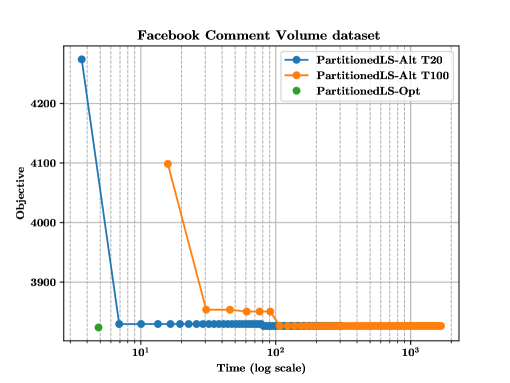
Figure 2: Plot of the behavior of the two proposed algorithms on the Facebook Comment Volume dataset. PartLS-alt has been repeated 100 times following a multi-start strategy and in two settings ($T$=20 and $T$=100). Each point on the orange and blue lines reports the cumulative time and best objective found during these 100 restarts.

5.3 Superconductivity dataset

The Superconductivity dataset contains 81 features representing characteristics of superconductors. The dataset contains $21264$ examples. In our experiment we trained the model over the first $10000$ examples. The task is to predict a material’s critical temperature. The features are derived from a superconductor’s atomic mass, density and fusion heat among others. We refer the reader to the original paper (Hamidieh, 2018) for the specific details about the process. In our experiment we created 7 feature blocks with 10 features each and an additional one which contained 11 features. PartLS-opt takes $\sim 47$ seconds reaching an objective value of $\sim 2051$. At about the same computational cost, PartLS-alt with $T=20$ reaches an objective of $\sim 2150$. It will take the algorithm about $\sim 440$ seconds to lower that figure to a loss objective value ($\sim 2072$) comparable to the one obtained by PartLS-opt. Setting $T=100$ slightly improves the situation: after about $40$ seconds the loss objective is $\sim 2117$, which lowers to $\sim 2080$ after $\sim 186$ seconds and to $\sim 2064$ after $\sim 881$ seconds.

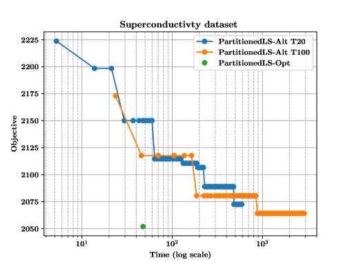
Figure 3: Plot of the behavior of the two proposed algorithms on the Superconductivty dataset. The PartLS-alt has been repeated 100 times following a multi-start strategy and in two settings ($T$=20 and $T$=100). Each point on the orange and blue lines reports the cumulative time and best objective found during these 100 restarts.

5.4 YearPredictionMSD Dataset

We also propose an experimentation on the YearPredictionMSD dataset. It is a subset of the Million Songs dataset (Bertin-Mahieux et al., 2011). When compared with the original dataset, it has about half the examples (around 500 thousand) and instead of the raw audio and metadata 90 timbre-related features are included. As for the Superconductivity dataset, we limited our experimentation to the first $10000$ examples. The target variable represents the year a song has been released in. In this dataset we experimented with 9 blocks of 10 to 12 features. PartLS-opt takes $\sim 130$ seconds to reach the optimal loss at $\sim 920$. PartLS-alt with $T=20$ is instead able to find a solution which is reasonably close ($\sim 922$) to the optimal one in a much shorter time (around 20 seconds). When $T=100$ is used instead, PartLS-alt reaches a reasonable approximation only after $\sim 178$ seconds.

Figure 4: Plot of the behavior of the two proposed algorithms on the YearPredictionMSD dataset. PartLS-alt has been repeated 100 times following a multi-start strategy and in two settings ($T$=20 and $T$=100). Each point on the orange and blue lines reports the cumulative time and best objective found during these 100 restarts.

5.5 Experiment Summary

The experiments confirm that PartLS-opt retrieves a more accurate solutions, as expected by its global optimality property as established in Section 3.2. Depending on the dataset, this solution can be cheaper or more costly to compute when compared to the approximate solution obtained by PartLS-alt. Indeed, it is straightforward to observe that, in typical scenarios, the alternating least squares approach, PartLS-alt, is able to outperform PartLS-opt in terms of running time only when the total number of iterations (and, thus, the total number of convex subproblems to be solved) is smaller than $2^{K}$, i.e., the number of subproblems solved by PartLS-opt to compute the optimal solution. In our experimentation, this leads to solutions that may grossly approximate the optimal one. Our conclusion is that PartLS-opt is likely to be preferable in most cases. It returns an optimal solution in a reasonable amount of time, often even lower than the time required by Algorithm 1. Also, while we observed that the alternating algorithm is sometimes able to retrieve faster than PartLS-opt a solution that could be “good enough”, its iterative nature can also lead to uncertainty.

Clearly there are cases where the number of groups or where the time required to solve a single convex problem is very large. In these cases, when approximate solutions are acceptable for the application at hand, PartLS-alt could be a very compelling solution. We conclude by noting that a use case with a large number of groups appears to us not very plausible. In fact, it could be argued that the reduced interpretability of the results defies the main motivation behind employing the Partitioned Least Squares model in the first place.

6 Conclusions

In this paper we presented an alternative least squares linear regression formulation. Our model enables scientists and practitioners to group features together into partitions, hence allowing the modeling of higher level abstractions which are easier to reason about. We provided rigorous proofs of the non-convexity of the problem and presented PartLS-alt and PartLS-opt, two algorithms to cope with the problem.

PartLS-alt is an iterative algorithm based on the alternating least squares method. The algorithm is proved to converge, but there is no guarantee that the accumulation point results in a globally optimal solution. On the contrary, as experiments have shown, the algorithm can be trapped in a local minimizer and return an approximate solution. Experiments suggest that it could be faster and preferable to PartLS-opt in some circumstances (e.g., when the time needed to solve a single sub-problem is large and the application allows for sub-optimal answers).

PartLS-opt is an enumerative, exact, algorithm and our contribution includes a formal optimality proof. In our experimentation, we confirmed that it behaves very well under several different settings, although its time complexity grows exponentially with the number of groups. We argue that this exponential growth in time complexity should not impede its adoption: a large number of groups seems implausible in practical scenarios since it would undermine interpretability of the results and hence the attractiveness of the problem formulation. However, for the sake of completeness and to provide guidance to the interested reader, we provided a branch-and-bound solution that shares the same optimality guarantees of PartLS-opt. This latter formulation, depending on the actual structure of the problem as implied by the data, might save computation by pruning the search space, possibly avoiding to solve a large number of sub-problems. We intend to investigate the possible runtime benefits of such a strategy in future work.

7 Reproducibility

A Julia (Bezanson et al., 2012) implementation of algorithms PartLS-alt and PartLS-alt is available at https://github.com/ml-unito/PartitionedLS; the code for the experiments is available at: https://github.com/ml-unito/PartitionedLS-experiments-2.
The repository for the experiments contains code to download and to pre-process the datasets (or the datasets themselves when not available for downloading) as well as the scripts to actually launch the experiments. Pre-processing consists in packing the data in a format suitable for the algorithms and to partition the data as mentioned in Section 5.

References

- Abdi [2010] Hervé Abdi. Partial least squares regression and projection on latent structure regression (PLS regression). WIREs Computational Statistics, 2(1), 2010.
- Bakin [1999] Sergey Bakin. Adaptive regression and model selection in data mining problems. PhD thesis, School of Mathematical Sciences, Australian National University, 1999.
- Bertin-Mahieux et al. [2011] Thierry Bertin-Mahieux, Daniel P. W. Ellis, Brian Whitman, and Paul Lamere. The million song dataset. In Proceedings of the 12th International Conference on Music Information Retrieval (ISMIR 2011), 2011.
- Bezanson et al. [2012] Jeff Bezanson, Stefan Karpinski, Viral B. Shah, and Adam Edelman. Julia: A fast dynamic language for technical computing. CoRR, 2012.
- Bro et al. [2002] Rasmus Bro, Nicholaos D. Sidiropoulos, and Age K. Smilde. Maximum likelihood fitting using ordinary least squares algorithms. Journal of Chemometrics: A Journal of the Chemometrics Society, 16(8-10), 2002.
- Caron et al. [2013] Giulia Caron, Maura Vallaro, and Giuseppe Ermondi. The block relevance (BR) analysis to aid medicinal chemists to determine and interpret lipophilicity. Med. Chem. Commun., 4, 2013.
- Caron et al. [2016] Giulia Caron, Maura Vallaro, Giuseppe Ermondi, Gilles H. Goetz, Yuriy A. Abramov, Laurence Philippe, and Marina Shalaeva. A fast chromatographic method for estimating lipophilicity and ionization in nonpolar membrane-like environment. Molecular Pharmaceutics, 13(3), 2016.
- Dua and Graff [2017] Dheeru Dua and Casey Graff. UCI machine learning repository, 2017. URL http://archive.ics.uci.edu/ml.
- Ermondi and Caron [2012] Giuseppe Ermondi and Giulia Caron. Molecular interaction fields based descriptors to interpret and compare chromatographic indexes. Journal of Chromatography A, 1252, 2012.
- Garey and Johnson [1979] M. R. Garey and D. S. Johnson. Computers and Intractability: A Guide to the Theory of NP-Completeness (Series of Books in the Mathematical Sciences). W. H. Freeman, 1979.
- Gauss [1995] Carl Friedrich Gauss. Theoria combinationis observationum erroribus minimis obnoxiae/theory of the combination of observations least subject to errors, volume 11 of classics in applied mathematics. Philadelphia, PA: Society for Industrial and Applied Mathematics, 1995. (Original work published 1821).
- Goodford [1985] P. J. Goodford. A computational procedure for determining energetically favorable binding sites on biologically important macromolecules. Journal of Medicinal Chemistry, 28(7), 1985.
- Gorski et al. [2007] Jochen Gorski, Frank Pfeuffer, and Kathrin Klamroth. Biconvex sets and optimization with biconvex functions: A survey and extensions. Mathematical Methods of Operations Research, 66, 2007.
- Hamidieh [2018] Kam Hamidieh. A data-driven statistical model for predicting the critical temperature of a superconductor. Computational Materials Science, 154:346–354, 2018.
- Huang et al. [2012] Jian Huang, Patrick Breheny, and Shuangge Ma. A selective review of group selection in high-dimensional models. Statistical science: a review journal of the Institute of Mathematical Statistics, 27(4), 2012.
- Intriligator et al. [1978] Michael D. Intriligator, Ronald G. Bodkin, and Cheng Hsiao. Econometric models, techniques, and applications. Prentice-Hall Englewood Cliffs, NJ, 1978.
- Isobe et al. [1990] Takashi Isobe, Eric D. Feigelson, Michael G. Akritas, and Gutti Jogesh Babu. Linear regression in astronomy. The astrophysical journal, 364, 1990.
- Lawler and Wood [1966] Eugene L. Lawler and David E. Wood. Branch-and-bound methods: A survey. Operations research, 14(4), 1966.
- Lawson and Hanson [1995] Charles L. Lawson and Richard J. Hanson. Solving least squares problems, volume 15. Siam, 1995.
- Lipton [2016] Zachary Lipton. The mythos of model interpretability. Communications of the ACM, 61, 2016.
- Nievergelt [2000] Yves Nievergelt. A tutorial history of least squares with applications to astronomy and geodesy. Journal of Computational and Applied Mathematics, 121(1), 2000.
- Reeder et al. [2004] Scott B. Reeder, Zhifei Wen, Huanzhou Yu, Angel R. Pineda, Garry E. Gold, Michael Markl, and Norbert J. Pelc. Multicoil dixon chemical species separation with an iterative least-squares estimation method. Magnetic Resonance in Medicine: An Official Journal of the International Society for Magnetic Resonance in Medicine, 51(1), 2004.
- Shor [1987] N. Z. Shor. Quadratic optimization problems. Soviet Journal of Computer and Systems Sciences, 25, 1987.
- Singh [2016] Kamaljot Singh. Facebook comment volume prediction. International Journal of Simulation- Systems, Science and Technology- IJSSST V16, 2016.
- Wendell and Hurter Jr. [1976] Richard E. Wendell and Arthur P. Hurter Jr. Minimization of a non-separable objective function subject to disjoint constraints. Operations Research, 24(4), 1976.
- Wold et al. [2001] Svante Wold, Michael Sjöström, and Lennart Eriksson. Pls-regression: a basic tool of chemometrics. Chemometrics and Intelligent Laboratory Systems, 58(2), 2001.
- Yuan and Lin [2006] Ming Yuan and Yi Lin. Model selection and estimation in regression with grouped variables. Journal of the Royal Statistical Society, Series B, 68:49–67, 2006.