Lepton Number Violating Electron Recoils in a $U(1)_{B-L}$ Model with Non-Standard Interactions

Abstract

We propose an $SU(3)_{C}\times SU(2)_{L}\times U(1)_{Y}\times U(1)_{B-L}$ model, in which the neutrino masses and mixings can be generated via Type-I seesaw mechanism after $U(1)_{B-L}$ breaking. A light mediator emerges and enables non-standard interaction that violates the lepton number. We show that the non-standard neutrino interaction emerges in this model, and it can lead to low energy recoil events with the solar neutrino flux. Analyses are performed with the keV range electron recoil events at recent direct detection experiments, including XENON1T, PANDAX and XENONnT. Recent direct detection observations lead to upper bound on the combined coupling strength to electron and neutrino to $\sqrt{y^{\prime}_{\nu}y_{e}}<0.5\times 10^{-6}$.

1 Introduction

Low-energy electron recoil received growing interest due to recent advances in direct detection with lowering thresholds  [1, 2, 3, 4, 5, 6, 7]. Recent keV range electron-recoil observations at XENON1T [8], PANDAX [9] and XENONnT [10], together with improved scrutiny on experimental radiative backgrounds, offer high-quality data for probing any new physics that leads to low-energy electron recoils, such as low-mass dark matter [11, 12], axions [13, 14, 15] and new interactions with neutrinos  [16, 17, 18, 19], etc. With new data in the keV range, recent new physics studies with electron recoils include tests of axion-like dark matter [20], solar axions [21, 22], non-standard neutrino interactions with light mediators [23, 24, 25, 26, 27, 28, 29, 30, 31], hidden photon dark matter [32, 33, 34], warm or fast moving dark matter [35] (also see [36]), boosted [37, 38, 39, 40, 41], inelastic or multi-component dark matter [42, 43, 44, 45, 46, 47], decaying dark matter [48, 49, 50], Migdal effect [51], luminous or shining dark matter [52, 53], inverse Primakoff effect [54], hydrogen decay [55], dark fluxes from accreting black holes [56], as well as re-examining detector backgrounds [57], collider searches [58], neutrino magnetic moment [59], stellar cooling [60, 61] limits, etc.

In this paper, we propose a $SU(3)_{C}\times SU(2)_{L}\times U(1)_{Y}\times U(1)_{B-L}$ model to derive low-energy electron recoils via non-standard neutrino-electron interactions with a light mediator. After the $U(1)_{B-L}$ breaking, the neutrino masses and mixings can be generated via the Type I seesaw mechanism. In particular, a light mediator exists in the model, as well as the non-standard interactions between the light mediator and leptons which violate the lepton number. Such light mediator would enhance the electron recoil rates at low energy region. We show that significant constraints on the model’s effective electron-neutrino couplings can be derived from the keV range electron recoil data from XENON1T, PANDAX and XENONnT.

2 Model Setup

The particles in the $SU(3)_{C}\times SU(2)_{L}\times U(1)_{Y}\times U(1)_{B-L}$ model follow the conventional notations that the Standard Model (SM) quark doublets $Q_{i}$, right-handed up-type quarks $U_{i}$, right-handed down-type quarks $D_{i}$, lepton doublets $L_{i}$, right-handed charged leptons $E_{i}$, and right-handed neutrinos $N_{i}^{c}$, with $i=1,2,3$ for three generations. Then we introduce new scalar fields, including one $SU(2)_{L}$ triplet $\Phi$, two $SU(2)_{L}$ doublets $H$ and $H^{\prime}$, and two SM singlets $S$ and $T$. The triplet and singlet fields are introduced to generate non-standard neutrino/lepton interactions, as will be discussed later. These particles and their quantum numbers under the $SU(3)_{C}\times SU(2)_{L}\times U(1)_{Y}\times U(1)_{B-L}$ gauge symmetry are summarized in Table 1.

	$SU(3)_{C}$	$SU(2)_{L}$	$U(1)_{Y}$	$U(1)_{B-L}$
$Q_{i}$	$\mathbf{3}$	$\mathbf{2}$	$\mathbf{1/6}$	$\mathbf{1/6}$
$U_{i}$	$\mathbf{{3}}$	$\mathbf{1}$	$\mathbf{2/3}$	$\mathbf{1/6}$
$D_{i}$	$\mathbf{{3}}$	$\mathbf{1}$	$\mathbf{-1/3}$	$\mathbf{1/6}$
$L_{i}$	$\mathbf{1}$	$\mathbf{2}$	$\mathbf{-1/2}$	$\mathbf{-1/2}$
$E_{i}$	$\mathbf{1}$	$\mathbf{1}$	$\mathbf{-1}$	$\mathbf{-1/2}$
$N_{i}$	$\mathbf{1}$	$\mathbf{1}$	$\mathbf{0}$	$\mathbf{-1/2}$
$XE$	$\mathbf{1}$	$\mathbf{1}$	$\mathbf{-1}$	$\mathbf{-3/2}$
$XE^{c}$	$\mathbf{1}$	$\mathbf{1}$	$\mathbf{1}$	$\mathbf{3/2}$
$\Phi$	$\mathbf{1}$	$\mathbf{3}$	$\mathbf{1}$	$\mathbf{1}$
$H$	$\mathbf{1}$	$\mathbf{2}$	$\mathbf{-1/2}$	$\mathbf{0}$
$H^{\prime}$	$\mathbf{1}$	$\mathbf{2}$	$\mathbf{-1/2}$	$\mathbf{-1}$
$S$	$\mathbf{1}$	$\mathbf{1}$	$\mathbf{0}$	$\mathbf{-1}$
$T$	$\mathbf{1}$	$\mathbf{1}$	$\mathbf{0}$	$\mathbf{-1}$

Table 1: Particles and their quantum numbers under the $SU(3)_{C}\times SU(2)_{L}\times U(1)_{Y}\times U(1)_{B-L}$ gauge group. $T$ and $H$ sequentially develop vev that break $U(1)_{B-L}$ and $SU(2)_{L}\times U(1)_{Y}$, respectively.

As we know, the $SU(3)_{C}\times SU(2)_{L}\times U(1)_{Y}\times U(1)_{B-L}$ gauge symmetry can be obtained from the $SO(10)$ gauge symmetry breaking. However, heavy $XE$, $XE^{c}$ fields, and the scalars $\Phi$, $H^{\prime}$, $S$, $T$ are not new particles in the traditional $SO(10)$ models. Interestingly, they can be obtained via the tensor products of the ${\mathbf{1}0}$ fundamental representation, as well as ${\mathbf{16}}$ and $\overline{\mathbf{16}}$ spinor representations of $SO(10)$, i.e., the higher representations of $SO(10)$ as follows

$$XE \subset \overline{\mathbf{16}}\otimes\overline{\mathbf{16}}\otimes\overline{\mathbf{16}}~{},~{}$$

$$XE^{c} \subset \mathbf{16}\otimes\mathbf{16}\otimes\mathbf{16}~{},~{}$$

$$\Phi \subset \mathbf{126}\subset\mathbf{16}\otimes\mathbf{16}~{},~{}$$

$$H^{\prime} \subset \mathbf{10}\otimes\overline{\mathbf{16}}\otimes\overline{\mathbf{16}}~{},~{}$$

$$S/T \subset \overline{\mathbf{120}}\subset\overline{\mathbf{16}}\otimes\overline{\mathbf{16}}~{}.~{}\,$$

We consider the $SU(3)_{C}\times SU(2)_{L}\times U(1)_{Y}\times U(1)_{B-L}$ groups as an intermediate stage of symmetry breaking sequence after the breaking of SO(10).

The $U(1)_{B-L}$ gauge symmetry spontaneously breaks after $T$ obtains a vacuum expectation value (vev), leaving out the SM $SU(3)_{C}\times SU(2)_{L}\times U(1)_{Y}$ at lower energy scales. $H$ is the SM Higgs doublet whose vev finally breaks the electroweak gauge symmetry, and we assume that $\Phi$, $H^{\prime}$ and $S$ do not acquire vevs. In particular, the effective Yukawa couplings between $H^{\prime}$ and charged leptons can be generated if we introduce a pair of vector-like particles $(XE,XE^{c})$ as heavy mediators and $\Phi$ can couple to lepton doublets as well. The $XE$ mass are generated by some UV symmetry breaking above the $U(1)_{B-L}$ scale. Because the CP-even neutral components of $\Phi$, $H^{\prime}$, and $S$ can mix with each other, their lightest mass eigenstate $s$ can couple to the charged leptons as well as neutrinos. In short, $T$ and $H$ are introduced to break the $U(1)_{B-L}$ gauge symmetry and electroweak gauge symmetry, respectively, while $\Phi$, $H^{\prime}$, and $S$ are introduced to generate the Yukawa couplings between the lightest CP-even neutral scalar and charged leptons/neutrinos.

Figure 1: Feynman diagram for the NSI $\nu e^{-}\rightarrow\nu^{c}e^{-}$ scattering.

The Lagrangian sector involving the fermions is

$$-{\cal L} = y_{ij}^{U}Q_{i}U_{j}^{c}\overline{H}+y_{ij}^{D}Q_{i}D_{j}^{c}H+y_{ij}^{E}L_{i}E_{j}^{c}H+y_{ij}^{\nu}L_{i}N_{j}^{c}\overline{H}$$ (1)

$$+y_{ij}^{N}TN_{i}^{c}N_{j}^{c}+y_{ij}^{\Phi}L_{i}\Phi L_{j}+y_{i}^{H^{\prime}}H^{\prime}L_{i}XE^{c}$$

$$+y_{i}^{T}\overline{T}E_{i}^{c}XE+M_{XE}XE^{c}XE+{\rm H.C.}~{},~{}\,$$

With the $y_{ij}^{\nu}L_{i}N_{j}^{c}\overline{H}$ and $y_{ij}^{N}TN_{i}^{c}N_{j}^{c}$ terms, we can generate the neutrino masses and mixings via Type I seesaw mechanism after $T$ acquires a vev and breaks the $U(1)_{B-L}$ gauge symmetry.

Now we can see non-standard neutrino interactions emerge from this model setup. The vector-like $(XE,XE^{c})$ masses are assumed heavy as the result of UV symmetry breaking. Integrating out $(XE,XE^{c})$, we can obtain effective operators,

$$-{\cal L}\supset-\frac{1}{M_{XE}}y_{i}^{H^{\prime}}y_{j}^{T}H^{\prime}\overline{T}L_{i}E_{j}^{c}+{\rm H.C.}~{}.~{}\,$$ (2)

After $U(1)_{B-L}$ gauge symmetry breaking, we get

$$-{\cal L}\supset-\frac{\langle\overline{T}\rangle}{M_{XE}}y_{i}^{H^{\prime}}y_{j}^{T}H^{\prime}L_{i}E_{j}^{c}+{\rm H.C.}~{}.~{}\,$$ (3)

For simplicity with phenomenology, we can assume that only $y_{1}^{H^{\prime}}$ and $y_{1}^{T}$ are non-zero. From the terms $y_{ij}^{\Phi}L_{i}\Phi L_{j}$ and Eq. (3), we obtain

$$-\mathcal{L}\ \supset\ \frac{y^{\prime\Phi}_{ij}}{2}\sin\alpha\cos\beta s_{1}\overline{\nu^{c}_{i}}\nu_{j}+y_{e}s_{1}\overline{e}e+{\rm H.C.}~{}~{}\,$$ (4)

where $\nu_{i}$ is the neutrino mass eigenstate, $e$ is the electron, $s_{1}$ is a CP-even mass eigenstate from ${S,\Phi,H^{\prime}}$ mixing, and

$$y_{e} = -\frac{\langle\overline{T}\rangle}{M_{XE}}y_{1}^{H^{\prime}}y_{1}^{T}\sin\alpha\sin\beta~{}.~{}\,$$ (5)

For a heavy $M_{\rm XE}$ mass much above $U(1)_{B-L}$ breaking scale the effective coupling $y_{e}$ can be naturally small. $\alpha,\beta$ denote the mixing angles from the neutral components in ${S,\Phi,H^{\prime}}$,

$$\left(\begin{array}[]{c}s_{1}\\ s_{2}\\ s_{3}\end{array}\right)=\left(\begin{array}[]{ccc}\cos\alpha&\sin\alpha\cos\beta&\sin\alpha\sin\beta\\ -\sin\alpha&\cos\alpha\cos\beta&\cos\alpha\sin\beta\\ 0&-\sin\beta&\cos\beta\end{array}\right){\rm Re}\left(\begin{array}[]{c}S\\ \Phi^{0}\\ H^{\prime 0}\end{array}\right).$$ (6)

$s_{1}$, $s_{2}$, $s_{3}$ are their mass eigenstate and we can take $s_{1}$ to be the lightest state,

$$s_{1}=\cos\alpha~{}{\rm Re}S+\sin\alpha\cos\beta~{}{\rm Re}\Phi^{0}+\sin\alpha\sin\beta~{}{\rm Re}H^{\prime 0}~{},~{}\,$$

from diagonalizing their mass matrix. Here, we can see the triplet $\Phi$ in this model is needed to generate the effective couplings between the light mediator $s_{1}$ and the neutrinos, the doublet field $H^{\prime}$ is needed to generate the effective couplings between $s_{1}$ and the charged leptons, and the singlet $S$ is needed to allow for a light mediator $s_{1}$.

Due to the number of scalar fields, this model has an extended scalar potential, and its general form can be written as

$$V = m_{S}^{2}|S|^{2}-m_{T}^{2}|T|^{2}-m_{H}^{2}|H|^{2}+m_{H^{\prime}}^{2}|H^{\prime}|^{2}+m_{\Phi}^{2}|\Phi|^{2}$$ (7)

$$+\lambda_{S}|S|^{4}+\lambda_{T}|T|^{4}+\lambda_{H}|H|^{4}+\lambda_{H^{\prime}}|H^{\prime}|^{4}+\lambda_{\Phi}|\Phi|^{4}$$

$$+\lambda_{ST}|S|^{2}|T|^{2}+\lambda_{SH}|S|^{2}|H|^{2}+\lambda_{SH^{\prime}}|S|^{2}|H^{\prime}|^{2}$$

$$+\lambda_{S\Phi}|S|^{2}|\Phi|^{2}+\lambda_{TH}|T|^{2}|H|^{2}+\lambda_{TH^{\prime}}|T|^{2}|H^{\prime}|^{2}$$

$$+\lambda_{T\Phi}|T|^{2}|\Phi|^{2}+\lambda_{HH^{\prime}}|H|^{2}|H^{\prime}|^{2}+\lambda_{H\Phi}|H|^{2}|\Phi|^{2}$$

$$+\lambda_{H^{\prime}\Phi}|H^{\prime}|^{2}|\Phi|^{2}+\left(A_{1}\Phi HH^{\prime}+A_{2}S\overline{H^{\prime}}H\right.$$

$$\left.+\lambda\Phi SHH+{\rm H.C.}\right)~{},~{}$$

where $\overline{H}=i\sigma_{2}H^{*}$ and $\overline{H^{\prime}}=i\sigma_{2}H^{\prime*}$ with $\sigma_{2}$ the second Pauli matrix, and we neglect the $T\overline{H^{\prime}}H$ and $\Phi THH$, which will induce the tadpole terms for $H^{\prime}$ and $\Phi$.

Here we need a light $s_{1}$ to mediate non-standard soft neutrino scattering that is relevant to electron recoils. In principle, because $S$ and $T$ carry the same quantum numbers, without loss of generality, we can make a $U(1)_{B-L}$ rotation so that only one linear combination of them has a vev in case they both have vevs. After $H$ and $T$ obtain vevs, the neutral components of $\Phi$, $S$, and $H^{\prime}$ fields will mix with each other, and we assume the lightest CP-even mass eigenstate to be very light in this paper. This typically would assume $V$ to be flat in some direction of Re$\{S,\Phi^{0},H^{\prime 0}\}$.

Before analysing the electron recoil phenomenology, we would like to emphasize the difference from the $SU(3)_{C}\times SU(2)_{L}\times U(1)_{I3R}\times U(1)_{B-L}$ model, i.e., the traditional $U(1)_{B-L}$ model [62, 63, 64, 65]. The main point is that $A_{1}\Phi HH^{\prime}$, $A_{2}S\overline{H^{\prime}}H$, and $\lambda\Phi SHH$ terms are necessary to generate the mixings among the neutral components of $\Phi$, $S$, and $H^{\prime}$, as well as $y_{ij}^{\Phi}L_{i}\Phi L_{j}$ to generate the $\frac{y^{\prime\Phi}_{ij}}{2}s\overline{\nu^{c}_{i}}\nu_{j}$ terms. In the traditional $SU(3)_{C}\times SU(2)_{L}\times U(1)_{I3R}\times U(1)_{B-L}$ model, the lepton doublets $L_{i}$ are charged under $U(1)_{B-L}$ while the Higgs field $H$ is neutral under $U(1)_{B-L}$. Thus, our model cannot be realized in the traditional $SU(3)_{C}\times SU(2)_{L}\times U(1)_{I3R}\times U(1)_{B-L}$ model.

3 Electron recoil

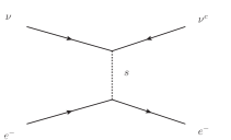
The $s_{1}\overline{\nu^{c}}\nu$ and $s_{1}\overline{e}e$ vertices in Eqs.3 and 4 allows $s_{1}$ to mediate ‘non-standard’ electron scattering process $\nu_{i}e^{-}\rightarrow\nu^{c}_{j}e^{-}$ as shown in Fig. 1. Since $s_{1}$ carries lepton number, this process violates the lepton number by two units, and has no corresponding diagrams in the SM. The scattering amplitude-square is

$$|{\cal M}|^{2}=-\frac{y_{\nu}^{\prime 2}y_{e}^{2}(4M_{e}^{2}-t)t}{(M_{s}^{2}-t)^{2}},$$ (8)

where $t=(p_{{\nu}^{c}}-p_{\nu})^{\mu}(p_{\nu^{c}}-p_{\nu})_{\mu}$ is the Mandelstam $t$ variable. Here we will denote $y^{\prime}_{\nu}\equiv\frac{y^{\prime\Phi}_{ij}}{2}\sin\alpha\cos\beta$ and neglect the flavor indices for convenience. For negligible neutrino masses, $t=-2M_{e}E_{k}$ for neutrinos scattering off a free electron, and the differential cross-section is

$$\frac{{\rm d}\sigma^{\nu e}}{{\rm d}E_{k}}=\frac{y^{\prime 2}y_{e}^{2}E_{k}M_{e}(E_{k}+2M_{e})}{8\pi E_{\nu}^{2}(M_{s}^{2}+2M_{e}E_{k})^{2}}.$$ (9)

$E_{k}$ is the electron’s acquired kinetic energy after scattering, and $E_{\nu}$ is the incident neutrino energy, see 21 for detail. Noted the $s_{1}\overline{\nu^{c}}\nu$ vertex leads to different scattering kinematics comparing to that from a lepton number conserving $s\overline{\nu}\nu$ vertex [16] at large momentum exchange, where the NSI scattering spectrum with the $s_{1}\overline{\nu^{c}}\nu$ vertex is harder at very large recoil energy $E_{k}\sim E_{\nu}$ and if $M_{s}$ were assumed heavy. However, since we are interested in keV recoils in this paper, the soft recoil spectra from these two types of vertices would converge and demonstrate a similar $E_{k}^{-1}$ behavior as long as $M_{s}$ is assumed smaller than the transfered momentum. In particular, it features a kinematic region:

$$M_{s}\ll\sqrt{2M_{e}E_{k}}\ll M_{e}.$$ (10)

Here low momentum transfer dominates the scattering as the cross-section in Eq. 9 behaves as $d\sigma/dE_{k}\propto E_{k}^{-1}$. For $s$ mass below the keV scale, Eq. 10 is typically satisfied by near-threshold (keV) energy transfer in electron recoil events with solar/reactor neutrinos at direct-detection experiments. Eq. 9 is for a free electron, and the differential rate for recoil energy $E_{R}$ would be

$$\frac{dN}{dE_{R}}=N\cdot T\cdot\epsilon(E_{R})\int{\rm d}E^{\prime}{\cal G}(E^{\prime},E_{R})\int{{\rm d}E_{\nu}}{\cal F}(E^{\prime})\frac{{\rm d}\phi_{\nu}}{{\rm d}E^{\prime}}\frac{{\rm d}\sigma^{\nu e}}{{\rm d}E^{\prime}},$$ (11)

where $N$ and $T$ are the number of targets and exposure time. For comparison with XENON1T results, $\epsilon$ is the detector efficiency [8]. ${\cal G}$ is a Gaussian smearing on $E_{R}$ that accounts for detector resolution,

$${\cal G}=\frac{1}{\sqrt{\pi}\delta_{E}}\exp^{-\frac{(E_{R}-E^{\prime})^{2}}{\delta_{E}^{2}}}$$ (12)

$\delta_{E}=\sqrt{0.31E}+0.0037E$, where $E$ is in keV, as given in Ref. [8]. $\phi_{\nu}$ is the Solar neutrino flux model that we adopt from Ref. [66]. ${\cal F}(E)=\sum_{i}\theta(E-B_{i})$ is the so-called ‘free electron approximation’ (FEA) that serves as the electron form factor with step-functions at binding energies in the ⁵⁴Xe atom as recoil thresholds. It physically represents the number of electrons that can be ionized at a given energy. FEA is adopted by XENON [8] and it gives a 10% correction on the $E_{R}\sim$keV recoil rate in our case. FEA is a popular approximation for recoil energies much higher than that of the atomic binding, and it has been shown to have very good agreement with amplitude-level photon-mediated form factor calculation for recoils at keV and above  [67, 68]. We use the FEA as a reasonable approximation to the level of a few percent for $E_{R}>$ keV, and an amplitude-level proof is of interest for future research.

Figure 2: Best-fit solar neutrino NSI event distribution (gray dotted) with $\sqrt{y_{\nu}y_{e}}={0.96}\times 10^{-6}$, background $\eta$B0 with $\eta=95.5\%$ (red dashed) and the total spectrum (solid). The NSI signal assumes the low $M_{s}$ limit ($M_{s}<$keV).

The $E_{R}^{-1}$ dependence from from light scalar mediated NSI leads to a relative moderate spectrum rise at the lowest energy bins, if compared to a more steep $E_{R}^{-2}$ dependence observed in light vector-boson mediated scenarios, as studied in Ref. [23, 24, 25, 26], etc. Note that photon-mediated BSM neutrino dipole interaction would also give an $E_{R}^{-1}$ dependence thus should yield similar explanation to data. In following sections we show the $s_{1}\overline{\nu^{c}}\nu$ NSI gives good fit the low energy electron recoils, and its significance is subject to effects from several SM radiative backgrounds.

4 Fit to XENON1T

The solar neutrino’s $\nu e\rightarrow\nu^{c}e$ event rate rises towards low energy, which is consistent with the electron recoil data reported by XENON1T. We make a likelihood fit to the 29 binned data [8] below 30 keV, by combining these NSI-induced events with XENON1T’s best-fit background modeling $B0$,

$$\chi^{2}=\sum_{i}\frac{(\eta B0_{i}+N_{i}^{e\nu}-N_{i}^{\rm data})^{2}}{(\delta N_{i})^{2}}+\frac{(1-\eta)^{2}}{(\delta\eta)^{2}},$$ (13)

where last term accounts for a small but crucial normalization uncertainty in the background model. In the low $E_{R}$ range, the detector background $B0$ is primarily the flat ²¹⁴Pb component, which is a calibrated in the entire 1-210 keV range and has a 2% statistic uncertainty. Detector efficiency modeling would contribute another 1% normalization uncertainty, and we take a combined $\delta\eta=3\%$.

Figure 3: Minimal $\chi^{2}$ after marginalizing over $\eta$. The $\sqrt{y_{\nu}y_{e}}\rightarrow 0$ direction approaches to the background-only fit. $5.8\times 10^{-7}<\sqrt{y_{\nu}y_{e}}<1.1\times 10^{-6}$ is a $2\sigma$ favored range around the best fit point. The shaded exclusion region is inferred from the BOREXINO bound [69].

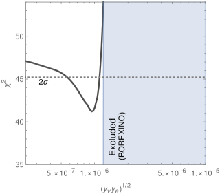
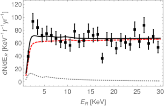
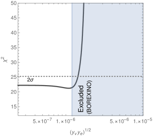
Best-fit spectra to XENON1T data is shown in Fig. 2. Taking the low $M_{s}$ limit ($M_{s}<$ keV), a minimal $\chi^{2}=41$ is obtained at $\sqrt{y_{\nu}y_{e}}={0.96}\times 10^{-6}$ with the background being slightly down-scaled at $\eta-1=-4.5\%$. The best fit point yields a $\Delta\chi^{2}=-6.7$ improvement over fixed $B0$ fit ($\eta=1$). The $\chi^{2}$ dependence on $\sqrt{y_{\nu}y_{e}}$ is plotted in Fig. 3 and the $2\sigma$-preference threshold around the best-fit $\sqrt{y_{\nu}y_{e}}$ is shown as the dotted curve. With 28 degrees of freedom, the minimal reduced $\chi^{2}/{dof\#}=1.46$ corresponds to 93% credence level (C.L.), which is not quite a perfect fit to the data below 30 keV. This is due to fluctuations above 10 keV that are still unaccounted for by the flat ²¹⁴Pb background and the NSI contribution close to the detector threshold.

Notably a trace abundance of tritium below calibrated level is not ruled out as a possibility to account for the keV range recoils [8]. The tritium induced recoil spectrum shape is similar to that from NSI and leads to degeneracy in explaining the low-energy rise. In the next session, we will show the NSI significance decreases after incorporating a more sophisticated radiative background model.

5 Fit to PANDAX

After XENON1T electron recoil data was reported, the PANDAX collaboration reported their data with 100.7 ton-day exposure and 2121 events selected [9]. There is also a rise at 3-7 keV. In contrast to the XENON experiment, more background were taken into account. Including tritium, ${}^{127}\mathrm{Xe}$, ${}^{85}\mathrm{Kr}$ and ${}^{222}\mathrm{Rn}$. We also make a likelihood fit to the 24 binned data below 25 keV, by combining these NSI-induced events with PANDAX’s best-fit background modeling,

$$\chi^{2} = \sum_{ij}\frac{(\eta_{j}B0_{ji}+N_{i}^{e\nu}-N_{i}^{\rm data})^{2}}{(\delta N_{i})^{2}}+\sum_{j}\frac{(1-\eta_{j})^{2}}{(\delta\eta_{j})^{2}}$$ (14)

where i denotes data point and $j=1,2,3,4$ denote ${}^{127}\mathrm{Xe}$, tritium, ${}^{85}\mathrm{Kr}$ and ${}^{222}\mathrm{Rn}$ background. Their best-fit value are respectively 80.8, 202.9, 1095, 735.6 [9]. $\eta$ is background floating parameters. Among this background, ${}^{127}\mathrm{Xe}$ and tritium were considered a major factor in low energy range electron recoil rise and their statistic uncertainty are $\delta\eta_{1}=21\%$, $\delta\eta_{2}=35\%$ [70]. The rest of them are considered mostly flat background which are calibrated at full energy region. Their statistic uncertainty is relatively much smaller than ${}^{127}\mathrm{Xe}$ and tritium so we don’t need to consider their float and set $\eta_{3}=\eta_{4}=1$. The PANDAX detector efficiency curve is taken from [71], which is degenerate with flat ${}^{222}\mathrm{Rn}$ background so the efficiency error is not also considered. Detector smearing curve is from [72], and we parameterized this curve as $\delta_{E}=0.2626\sqrt{E}+0.0426E$ where $E$ is in keV.

Figure 4: Best-fit new physics event distribution (gray dotted) with $\sqrt{y_{\nu}y_{e}}={1.1}\times 10^{-6}$, background ${}^{127}\mathrm{Xe}$ with $\eta_{1}=102.3\%$ and tritium with $\eta_{2}=93.3\%$. Electron recoil events are the total 100.7 ton-day data [9].

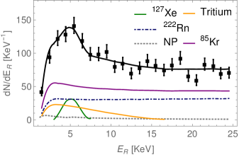
Fitting PANDAX data is shown in Fig. 4. The gray dotted line represent new physical signal with best-fit result. The background ${}^{127}\mathrm{Xe}$ is up-scaled at $\eta_{1}-1=2.3\%$ and tritium is down-scaled at $\eta_{2}-1=-6.7\%$. The $\chi^{2}$ dependence on $\sqrt{y_{\nu}y_{e}}$ is plotted in Fig. 5. A minimal $\chi^{2}=21.2$ is obtained at $\sqrt{y_{\nu}y_{e}}={1.1}\times 10^{-6}$ and this point yields a $\Delta\chi^{2}=-1.6$ improvement over background-only fitting results ($\chi^{2}=22.8$). The $2\sigma$-preference threshold around the best-fit $\sqrt{y_{\nu}y_{e}}$ is shown as the dotted curve. As PANDAX considered more background channels, the low energy range electron recoil rise can be explained well with background-only fit. Our new physical contribution is consistent with background-only fit, and we can constrain the NSI coupling to $\sqrt{y_{\nu}y_{e}}<1.4\times 10^{-6}$.

Figure 5: Minimal $\chi^{2}$ after marginalizing over $\eta_{j}$. $\sqrt{y_{\nu}y_{e}}<1.4\times 10^{-6}$ is $2\sigma$ favored range and consistent with background-only fit to PANDAX data. The shaded exclusion region is inferred from the BOREXINO bound [69].

6 Fit to XENONnT

Recently, XENONnT released the newest data with the larger exposure of 1.16 ton-years and lower background rate [10]. In the XENONnT experiment, they have improved systematics and achieved more than 50% background reduction. The excess reported in XENON1T may be from trace amount of tritium and they can’t confirm or exclude it at that time. At the XENONnT experiment, they have successfully excluded the tritium component in the background model. Besides, the dominative low-energy background ${}^{214}\mathrm{Pb}$ in XENON1T, a $\beta$-emitter from ${}^{222}\mathrm{Rn}$, have been further reduced in XENONnT by a new high-flow radon removal system [73]. The XENONnT experiment includes nine components in the benchmark background model B0 throughout the 1-140 keV region. The main background sources below 30 keV are ${}^{214}\mathrm{Pb}$, ${}^{136}\mathrm{Xe}$, ${}^{85}\mathrm{Kr}$ and materials [10]. Unlike XENON1T, there is no obvious excess to be observed above the background at electron recoil energy below 7 keV.

Considering the major background’s spectral shape is not degenerate with that of our new physical signal, here we do not need to decompose the background and will use the overall background ‘B0’ in our analysis. We will allow this background to float by an $\eta$ parameter with an uncertainty $\delta\eta=3\%$ that corresponds to a background-only fit. Our fitting likelihood is

$$\chi^{2}=\sum_{i}\frac{(\eta B0_{i}+N_{i}^{e\nu}-N_{i}^{\rm data})^{2}}{(\delta N_{i})^{2}}+\frac{(1-\eta)^{2}}{(\delta\eta)^{2}},$$ (15)

which fit to XENONnT’s 29 binned data below 30 keV.

Figure 6: Minimal $\chi^{2}$ after marginalizing over floating parameters $\eta$. $\sqrt{y_{\nu}y_{e}}<0.56\times 10^{-6}$ is $2\sigma$ favored range and consistent with background-only fit to XENONnT data. The shaded exclusion region is inferred from the BOREXINO bound [69].

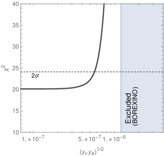
By combining the new physical contribution and XENONnT’s newest data below 30 keV from ref. [10], we can get the corresponding limits of scalar coupling. The $\chi^{2}$ dependence on $\sqrt{y_{\nu}y_{e}}$ is plotted in Fig. 6. There is no obvious minimal $\chi^{2}$ which is nearly a constant $\chi^{2}$=20.1 in the $\sqrt{y_{\nu}y_{e}}\rightarrow 0$ direction. In other words, the new physical contribution is also consistent with background-only fit. The $2\sigma$-preference threshold around the $\sqrt{y_{\nu}y_{e}}$ is shown as the dotted curve and we can get the limit of NSI coupling $\sqrt{y_{\nu}y_{e}}<0.56\times 10^{-6}$. It is clear that comparing with previous electron recoil results, XENONnT experiment gives the strongest constraint on the combined $e,\nu$ couplings to the light scalar in our model.

7 Comparisons & Discussion

A few comments are due for comparing the result from lepton-number violating scattering to those existing constraints at solar and reactor neutrino experiments. As long as Eq. 10 is satisfied, $d\sigma/dE_{R}\propto E_{R}^{-1}$ is a common kinematic feature that is also observed in lepton-number conserving ($s\overline{\nu}\nu$) scalar and neutrino magnetic dipole moment [74, 75, 76] scenarios. As most signal events are expected to be near-threshold, $s\overline{\nu}\nu$, $s\overline{\nu^{c}}\nu$ and $\overline{\nu}\sigma_{\mu\nu}\nu F^{\mu\nu}$ operators will lead to almost identical event distributions. This allows the scalar coupling bounds to be directly scaled from the existing $\nu_{\mu}$ limits. For instance, the signal events with $\nu_{\mu}=2.8\times 10^{-11}\mu_{\rm B}$, which corresponds to BOREXINO [69] bounds, shown as the shaded exclusion in Fig. 3. If we do not include a tritium component, the fit to XENON1T gives a slightly ($2\sigma$) favored range $5.8\times 10^{-7}<\sqrt{y_{\nu}y_{e}}<1.1\times 10^{-6}$ just below the BOREXINO exclusion upper bound.

Given the null results from following measurements, fits to XENON1T, PANDAX, and XENONnT can also be interpreted as stringent constraints on $\sqrt{y_{\nu}y_{e}}$ that are comparable to similar experimental results. As shown in Fig. 3,  5 and  6, assuming null-signal the new scalar coupling $\sqrt{y_{\nu}y_{e}}$ is constrained to be below $1.1\times 10^{-6}$, $1.4\times 10^{-6}$, $0.5\times 10^{-6}$ respectively. Beside BOREXINO, there are non-standard lectron-neutrino interaction limits from several other neutrino experiments, such as GEMMA [77], TEXONO [78] and CHARM-II [79], with GEMMA and BOREXINO providing the most stringent constraints. For comparison, NSI scattering with a similar $E_{R}^{-1}$ low-energy dependence can be interpreted from Ref. [24, 31], yielding a light scalar coupling limit $\sqrt{y_{\nu}y_{e}}\lesssim 1.2\times 10^{-6}$. We can see these limits largely fall in a very close range, with XENONnT giving the strongest constraint among these experiments, followed by the constraints is from XENON1T, GEMMA and BOREXINO, and then PANDAX.

As reactor neutrino is predominantly $\overline{\nu}_{e}$ at short distances, reactor neutrino constraints can be circumvented by assuming $y^{\nu}_{ij}$ in Eq. 4 only involve $\nu_{\mu}$ and $\nu_{\tau}$, at the cost of raising the average $\sqrt{y_{\nu_{\mu}}y_{e}},\sqrt{y_{\nu_{\tau}}y_{e}}$ by approximately 10%-19% as $\nu_{e}$ makes $1/3$ to $1/2$ of the solar neutrino flux [80] after flavor oscillation in the Sun. Note solar neutrino experimental bounds would also relax accordingly.

Since the light scalar couples to both neutrinos and electrons by effective operators at low energy scale, it can be emitted by hot electrons and neutrinos inside dense environments, hence such couplings are subject to stellar cooling constraints. For $M_{s}\ll$ keV, $y_{\nu}\leq 10^{-6}$ is still consistent with stellar cooling bounds [81]. However, the electron coupling $y_{e}$ would be severely constrained. For instance, Ref. [82] suggested a $y_{e}\lesssim 10^{-14}$ bound for a scalar-electron type coupling, and similar studies [60] gives a $y_{e}\lesssim 10^{-12}$ constraint. These astrophysical bounds prevent the product $\sqrt{y_{\nu}y_{e}}$ from reaching the $10^{-6}$ level.There are proposals to circumvent the stellar cooling bound, e.g. chameleon scenario(s) where the mediator acquires environment-dependent masses [83, 84, 85]. Realizing such scenarios requires more sophisticated model structure and is of interest for future research.

8 Conclusion

In this paper, we propose a model in the $SU(3)_{C}\times SU(2)_{L}\times U(1)_{Y}\times U(1)_{B-L}$ framework that provides a light scalar $s_{1}$ after $U(1)_{\rm B-L}$ and electroweak symmetry breaking, and also generates $s_{1}\overline{\nu^{c}}\nu$, $s\overline{e}e$ couplings via heavy fields above the $U(1)_{\rm B-L}$ breaking scale. These couplings violate lepton number and lead to non-standard $\nu e\rightarrow\nu^{c}e$ scattering. Solar MeV neutrinos may scatter off detector’s electron via the non-standard electron-neutrino interaction, and will enhance low $E_{R}$ electron recoil event rate.

We calculate the recoil spectrum for Solar neutrino’s $\nu e\rightarrow\nu^{c}e$ process, and compare the NSI spectrum in the light mediator limit ($M_{s}$ below keV) to other scattering processes, which share a common $E_{R}^{-1}$ kinematic feature near the recoil threshold energy. XENON1T data prefer a coupling range $5.8\times 10^{-7}<\sqrt{y_{\nu}y_{e}}<1.1\times 10^{-6}$, by fitting to the binned with a $3\%$ uncertainty on the ²¹⁴Pb dominated background and detector efficiency. In principle this fit can be degenerate with a trace-level of tritium background. Such a $\sqrt{y_{\nu}y_{e}}$ range is consistent with existing solar neutrino measurements, and by assuming flavored $\nu_{\mu},\nu_{\tau}$ couplings, avoids the bounds from reactor neutrino experiments, yet it is subject to rather severe $y_{e}$ constraint from stellar cooling, and may requires more sophisticated scenario of the mediator to comply with astrophysical limits.

The NSI-induced event rise towards the lower energy bins also allow very stringent constraints to be placed the NSI couplings. For PANDAX, the SM backgrounds including tritium and ¹²⁷Xe provide excellent fit to the shape of the electron recoil spectrum. Inclusion of the light $s_{1}$ mediated NSI signal only yields a slight improvement and is consistent with a background only fit. PANDAX data requires $\sqrt{y_{\nu}y_{e}}<1.4\times 10^{-6}$ that is close to reactor experiment limits. In addition, the fit to XENONnT data can constrain the NSI couplings to $\sqrt{y_{\nu}y_{e}}<0.56\times 10^{-6}$, which is the strongest among terrestrial low-energy recoil and neutrino experiments.

Acknowledgments

The authors thank K. Ni, J. Ye and X. Zhou for helpful discussions with the XENON1T background modeling, and PANDAX detector efficiency and smearing. Authors also thank B. Dutta and S. Ghosh for discussions. Y.G. is partially supported by the National R&D Program of China, 2020YFC2201601. T.L. is supported in part by the Projects 11875062 and 11947302 supported by the National Natural Science Foundation of China, and by the Key Research Program of Frontier Science, CAS.

Appendix A $s\overline{\nu^{c}}\nu$ Scattering Amplitude

For the $s\overline{\nu^{c}}\nu$ scattering on electrons, the amplitude is

$$i\mathcal{M}=i\frac{y_{\nu}^{\prime}y_{e}}{(p_{4}-p_{2})^{2}-M_{s}^{2}}\bar{u}(p_{4})u(p_{2})\bar{u}(p_{3})u(p_{1}),$$ (16)

$p_{1}$, $p_{3}$ are the initial and recoil electron 4-momenta. $p_{2}$, $p_{4}$ are the incident and ejected neutrino 4-momenta. The amplitude-square is

$$|\mathcal{M}|^{2} =\frac{y_{\nu}^{\prime 2}y_{e}^{2}}{4(M_{s}^{2}-t)^{2}}\operatorname{tr}[\not p_{4}\not p_{2}]\operatorname{tr}[(\not p_{3}+M_{e})(\not p_{1}+M_{e})]$$ (17)

$$=\frac{y_{\nu}^{\prime 2}y_{e}^{2}}{4(M_{s}^{2}-t)^{2}}(4p_{2}\cdot p_{4})(4p_{1}\cdot p_{3}+4M_{e}^{2}).$$

Using $p_{2}\cdot p_{4}=-\frac{1}{2}t$, $p_{1}\cdot p_{3}=M_{e}^{2}+M_{e}E_{k}=M_{e}^{2}-\frac{1}{2}t$, where $t$ is the Mandelstam variable which is defined in the main text, then we get

$$|\mathcal{M}|^{2}=-\frac{y_{\nu}^{\prime 2}y_{e}^{2}\left(4M_{e}^{2}-t\right)t}{\left(M_{s}^{2}-t\right)^{2}}.$$ (18)

In the lab frame, the total cross-section is

$$\sigma=\frac{1}{4M_{e}E_{\nu}}\int\frac{d^{3}\vec{p}_{3}d^{3}\vec{p}_{4}}{(2\pi)^{6}2E_{3}2E_{4}}(2\pi)^{4}\delta^{4}(p_{1}+p_{2}-p_{3}-p_{4})|\mathcal{M}|^{2}.$$ (19)

Integrating out $p_{4}$, we have

$$\sigma=\frac{1}{4M_{e}E_{\nu}}\int\frac{dE_{3}}{8\pi|\vec{p}_{2}|}|\mathcal{M}|^{2},$$ (20)

$E_{3}=M_{e}+E_{k}$, $|\vec{p}_{2}|=E_{\nu}$, where $E_{k}$ is the electron’s acquired kinetic energy after scattering. The differential cross-section is

$$\frac{d\sigma}{dE_{k}} =\frac{1}{4M_{e}E_{\nu}}\cdot\frac{1}{8\pi|\vec{p}_{2}|}\cdot|\mathcal{M}|^{2}$$ (21)

$$=\frac{y^{\prime 2}y_{e}^{2}E_{k}M_{e}\left(E_{k}+2M_{e}\right)}{8\pi E_{\nu}^{2}\left(M_{s}^{2}+2M_{e}E_{k}\right)^{2}},$$

as in Eq. 9.

References

- [1] E. Aprile, et al., Physics reach of the XENON1T dark matter experiment, JCAP 04 (2016) 027. arXiv:1512.07501, doi:10.1088/1475-7516/2016/04/027.
- [2] J. Aalbers, et al., DARWIN: towards the ultimate dark matter detector, JCAP 11 (2016) 017. arXiv:1606.07001, doi:10.1088/1475-7516/2016/11/017.
- [3] C. E. Aalseth, et al., DarkSide-20k: A 20 tonne two-phase LAr TPC for direct dark matter detection at LNGS, Eur. Phys. J. Plus 133 (2018) 131. arXiv:1707.08145, doi:10.1140/epjp/i2018-11973-4.
- [4] D. S. Akerib, et al., Projected WIMP sensitivity of the LUX-ZEPLIN dark matter experiment, Phys. Rev. D 101 (5) (2020) 052002. arXiv:1802.06039, doi:10.1103/PhysRevD.101.052002.
- [5] M. Schumann, L. Baudis, L. Bütikofer, A. Kish, M. Selvi, Dark matter sensitivity of multi-ton liquid xenon detectors, JCAP 10 (2015) 016. arXiv:1506.08309, doi:10.1088/1475-7516/2015/10/016.
- [6] L. Barak, et al., SENSEI: Direct-Detection Results on sub-GeV Dark Matter from a New Skipper-CCD, Phys. Rev. Lett. 125 (17) (2020) 171802. arXiv:2004.11378, doi:10.1103/PhysRevLett.125.171802.
- [7] R. Agnese, et al., New Results from the Search for Low-Mass Weakly Interacting Massive Particles with the CDMS Low Ionization Threshold Experiment, Phys. Rev. Lett. 116 (7) (2016) 071301. arXiv:1509.02448, doi:10.1103/PhysRevLett.116.071301.
- [8] E. Aprile, et al., Excess electronic recoil events in XENON1T, Phys. Rev. D 102 (7) (2020) 072004. arXiv:2006.09721, doi:10.1103/PhysRevD.102.072004.
- [9] X. Zhou, et al., A search for solar axions and anomalous neutrino magnetic moment with the complete PandaX-II data (8 2020). arXiv:2008.06485, doi:10.1088/0256-307X/38/1/011301.
- [10] E. Aprile, et al., Search for New Physics in Electronic Recoil Data from XENONnT, Phys. Rev. Lett. 129 (16) (2022) 161805. arXiv:2207.11330, doi:10.1103/PhysRevLett.129.161805.
- [11] R. Essig, J. Mardon, T. Volansky, Direct Detection of Sub-GeV Dark Matter, Phys. Rev. D 85 (2012) 076007. arXiv:1108.5383, doi:10.1103/PhysRevD.85.076007.
- [12] T. Bringmann, M. Pospelov, Novel direct detection constraints on light dark matter, Phys. Rev. Lett. 122 (17) (2019) 171801. arXiv:1810.10543, doi:10.1103/PhysRevLett.122.171801.
- [13] A. H. Córsico, L. G. Althaus, M. M. Miller Bertolami, S. Kepler, E. García-Berro, Constraining the neutrino magnetic dipole moment from white dwarf pulsations, JCAP 08 (2014) 054. arXiv:1406.6034, doi:10.1088/1475-7516/2014/08/054.
- [14] M. Giannotti, I. G. Irastorza, J. Redondo, A. Ringwald, K. Saikawa, Stellar Recipes for Axion Hunters, JCAP 10 (2017) 010. arXiv:1708.02111, doi:10.1088/1475-7516/2017/10/010.
- [15] S. A. Díaz, K.-P. Schröder, K. Zuber, D. Jack, E. E. B. Barrios, Constraint on the axion-electron coupling constant and the neutrino magnetic dipole moment by using the tip-RGB luminosity of fifty globular clusters (10 2019). arXiv:1910.10568.
- [16] D. G. Cerdeño, M. Fairbairn, T. Jubb, P. A. N. Machado, A. C. Vincent, C. Bœhm, Physics from solar neutrinos in dark matter direct detection experiments, JHEP 05 (2016) 118, [Erratum: JHEP 09, 048 (2016)]. arXiv:1604.01025, doi:10.1007/JHEP09(2016)048.
- [17] B. Dutta, S. Liao, L. E. Strigari, J. W. Walker, Non-standard interactions of solar neutrinos in dark matter experiments, Phys. Lett. B 773 (2017) 242–246. arXiv:1705.00661, doi:10.1016/j.physletb.2017.08.031.
- [18] D. Aristizabal Sierra, N. Rojas, M. H. G. Tytgat, Neutrino non-standard interactions and dark matter searches with multi-ton scale detectors, JHEP 03 (2018) 197. arXiv:1712.09667, doi:10.1007/JHEP03(2018)197.
- [19] M. C. Gonzalez-Garcia, M. Maltoni, Y. F. Perez-Gonzalez, R. Zukanovich Funchal, Neutrino Discovery Limit of Dark Matter Direct Detection Experiments in the Presence of Non-Standard Interactions, JHEP 07 (2018) 019. arXiv:1803.03650, doi:10.1007/JHEP07(2018)019.
- [20] F. Takahashi, M. Yamada, W. Yin, XENON1T Excess from Anomaly-Free Axionlike Dark Matter and Its Implications for Stellar Cooling Anomaly, Phys. Rev. Lett. 125 (16) (2020) 161801. arXiv:2006.10035, doi:10.1103/PhysRevLett.125.161801.
- [21] L. Di Luzio, M. Fedele, M. Giannotti, F. Mescia, E. Nardi, Solar axions cannot explain the XENON1T excess, Phys. Rev. Lett. 125 (13) (2020) 131804. arXiv:2006.12487, doi:10.1103/PhysRevLett.125.131804.
- [22] C. Gao, J. Liu, L.-T. Wang, X.-P. Wang, W. Xue, Y.-M. Zhong, Reexamining the Solar Axion Explanation for the XENON1T Excess, Phys. Rev. Lett. 125 (13) (2020) 131806. arXiv:2006.14598, doi:10.1103/PhysRevLett.125.131806.
- [23] D. W. P. d. Amaral, D. G. Cerdeno, P. Foldenauer, E. Reid, Solar neutrino probes of the muon anomalous magnetic moment in the gauged , JHEP 12 (2020) 155. arXiv:2006.11225, doi:10.1007/JHEP12(2020)155.
- [24] C. Boehm, D. G. Cerdeno, M. Fairbairn, P. A. N. Machado, A. C. Vincent, Light new physics in XENON1T, Phys. Rev. D 102 (2020) 115013. arXiv:2006.11250, doi:10.1103/PhysRevD.102.115013.
- [25] A. Bally, S. Jana, A. Trautner, Neutrino self-interactions and XENON1T electron recoil excess, Phys. Rev. Lett. 125 (16) (2020) 161802. arXiv:2006.11919, doi:10.1103/PhysRevLett.125.161802.
- [26] D. Aristizabal Sierra, V. De Romeri, L. J. Flores, D. K. Papoulias, Light vector mediators facing XENON1T data, Phys. Lett. B 809 (2020) 135681. arXiv:2006.12457, doi:10.1016/j.physletb.2020.135681.
- [27] A. N. Khan, Can Nonstandard Neutrino Interactions explain the XENON1T spectral excess?, Phys. Lett. B 809 (2020) 135782. arXiv:2006.12887, doi:10.1016/j.physletb.2020.135782.
- [28] H. An, M. Pospelov, J. Pradler, A. Ritz, New limits on dark photons from solar emission and keV scale dark matter, Phys. Rev. D 102 (2020) 115022. arXiv:2006.13929, doi:10.1103/PhysRevD.102.115022.
- [29] L. Zu, G.-W. Yuan, L. Feng, Y.-Z. Fan, Mirror Dark Matter and Electronic Recoil Events in XENON1T, Nucl. Phys. B 965 (2021) 115369. arXiv:2006.14577, doi:10.1016/j.nuclphysb.2021.115369.
- [30] M. Lindner, Y. Mambrini, T. B. de Melo, F. S. Queiroz, XENON1T anomaly: A light Z’ from a Two Higgs Doublet Model, Phys. Lett. B 811 (2020) 135972. arXiv:2006.14590, doi:10.1016/j.physletb.2020.135972.
- [31] A. N. Khan, Constraints on General Light Mediators from PandaX-II Electron Recoil Data, Phys. Lett. B 819 (2021) 136415. arXiv:2008.10279, doi:10.1016/j.physletb.2021.136415.
- [32] G. Alonso-Álvarez, F. Ertas, J. Jaeckel, F. Kahlhoefer, L. J. Thormaehlen, Hidden Photon Dark Matter in the Light of XENON1T and Stellar Cooling, JCAP 11 (2020) 029. arXiv:2006.11243, doi:10.1088/1475-7516/2020/11/029.
- [33] K. Nakayama, Y. Tang, Gravitational Production of Hidden Photon Dark Matter in Light of the XENON1T Excess, Phys. Lett. B 811 (2020) 135977. arXiv:2006.13159, doi:10.1016/j.physletb.2020.135977.
- [34] I. M. Bloch, A. Caputo, R. Essig, D. Redigolo, M. Sholapurkar, T. Volansky, Exploring new physics with O(keV) electron recoils in direct detection experiments, JHEP 01 (2021) 178. arXiv:2006.14521, doi:10.1007/JHEP01(2021)178.
- [35] K. Kannike, M. Raidal, H. Veermäe, A. Strumia, D. Teresi, Dark Matter and the XENON1T electron recoil excess, Phys. Rev. D 102 (9) (2020) 095002. arXiv:2006.10735, doi:10.1103/PhysRevD.102.095002.
- [36] M. D. Campos, W. Rodejohann, Testing keV sterile neutrino dark matter in future direct detection experiments, Phys. Rev. D 94 (9) (2016) 095010. arXiv:1605.02918, doi:10.1103/PhysRevD.94.095010.
- [37] B. Fornal, P. Sandick, J. Shu, M. Su, Y. Zhao, Boosted Dark Matter Interpretation of the XENON1T Excess, Phys. Rev. Lett. 125 (16) (2020) 161804. arXiv:2006.11264, doi:10.1103/PhysRevLett.125.161804.
- [38] Y. Chen, M.-Y. Cui, J. Shu, X. Xue, G.-W. Yuan, Q. Yuan, Sun heated MeV-scale dark matter and the XENON1T electron recoil excess, JHEP 04 (2021) 282. arXiv:2006.12447, doi:10.1007/JHEP04(2021)282.
- [39] Q.-H. Cao, R. Ding, Q.-F. Xiang, Searching for sub-MeV boosted dark matter from xenon electron direct detection, Chin. Phys. C 45 (4) (2021) 045002. arXiv:2006.12767, doi:10.1088/1674-1137/abe195.
- [40] Y. Jho, J.-C. Park, S. C. Park, P.-Y. Tseng, Leptonic New Force and Cosmic-ray Boosted Dark Matter for the XENON1T Excess, Phys. Lett. B 811 (2020) 135863. arXiv:2006.13910, doi:10.1016/j.physletb.2020.135863.
- [41] Y. Jho, J.-C. Park, S. C. Park, P.-Y. Tseng, Cosmic-Neutrino-Boosted Dark Matter (BDM) (1 2021). arXiv:2101.11262.
- [42] K. Harigaya, Y. Nakai, M. Suzuki, Inelastic Dark Matter Electron Scattering and the XENON1T Excess, Phys. Lett. B 809 (2020) 135729. arXiv:2006.11938, doi:10.1016/j.physletb.2020.135729.
- [43] L. Su, W. Wang, L. Wu, J. M. Yang, B. Zhu, Atmospheric Dark Matter and Xenon1T Excess, Phys. Rev. D 102 (11) (2020) 115028. arXiv:2006.11837, doi:10.1103/PhysRevD.102.115028.
- [44] H. M. Lee, Exothermic dark matter for XENON1T excess, JHEP 01 (2021) 019. arXiv:2006.13183, doi:10.1007/JHEP01(2021)019.
- [45] J. Bramante, N. Song, Electric But Not Eclectic: Thermal Relic Dark Matter for the XENON1T Excess, Phys. Rev. Lett. 125 (16) (2020) 161805. arXiv:2006.14089, doi:10.1103/PhysRevLett.125.161805.
- [46] M. Baryakhtar, A. Berlin, H. Liu, N. Weiner, Electromagnetic Signals of Inelastic Dark Matter Scattering (6 2020). arXiv:2006.13918.
- [47] H.-J. He, Y.-C. Wang, J. Zheng, GeV Scale Inelastic Dark Matter with Dark Photon Mediator via Direct Detection and Cosmological/Laboratory Constraints (12 2020). arXiv:2012.05891.
- [48] M. Du, J. Liang, Z. Liu, V. Q. Tran, Y. Xue, On-shell mediator dark matter models and the Xenon1T excess, Chin. Phys. C 45 (1) (2021) 013114. arXiv:2006.11949, doi:10.1088/1674-1137/abc244.
- [49] G. Choi, M. Suzuki, T. T. Yanagida, XENON1T Anomaly and its Implication for Decaying Warm Dark Matter, Phys. Lett. B 811 (2020) 135976. arXiv:2006.12348, doi:10.1016/j.physletb.2020.135976.
- [50] J. Buch, M. A. Buen-Abad, J. Fan, J. S. C. Leung, Galactic Origin of Relativistic Bosons and XENON1T Excess, JCAP 10 (2020) 051. arXiv:2006.12488, doi:10.1088/1475-7516/2020/10/051.
- [51] U. K. Dey, T. N. Maity, T. S. Ray, Prospects of Migdal Effect in the Explanation of XENON1T Electron Recoil Excess, Phys. Lett. B 811 (2020) 135900. arXiv:2006.12529, doi:10.1016/j.physletb.2020.135900.
- [52] N. F. Bell, J. B. Dent, B. Dutta, S. Ghosh, J. Kumar, J. L. Newstead, Explaining the XENON1T excess with Luminous Dark Matter, Phys. Rev. Lett. 125 (16) (2020) 161803. arXiv:2006.12461, doi:10.1103/PhysRevLett.125.161803.
- [53] G. Paz, A. A. Petrov, M. Tammaro, J. Zupan, Shining dark matter in Xenon1T, Phys. Rev. D 103 (5) (2021) L051703. arXiv:2006.12462, doi:10.1103/PhysRevD.103.L051703.
- [54] J. B. Dent, B. Dutta, J. L. Newstead, A. Thompson, Inverse Primakoff Scattering as a Probe of Solar Axions at Liquid Xenon Direct Detection Experiments, Phys. Rev. Lett. 125 (13) (2020) 131805. arXiv:2006.15118, doi:10.1103/PhysRevLett.125.131805.
- [55] D. McKeen, M. Pospelov, N. Raj, Hydrogen Portal to Exotic Radioactivity, Phys. Rev. Lett. 125 (23) (2020) 231803. arXiv:2006.15140, doi:10.1103/PhysRevLett.125.231803.
- [56] R.-G. Cai, S. Sun, B. Zhang, Y.-L. Zhang, Dark Fluxes from Accreting Black Holes and Direct Detections (9 2020). arXiv:2009.02315.
- [57] A. E. Robinson, XENON1T observes tritium (6 2020). arXiv:2006.13278.
- [58] R. Primulando, J. Julio, P. Uttayarat, Collider Constraints on a Dark Matter Interpretation of the XENON1T Excess, Eur. Phys. J. C 80 (11) (2020) 1084. arXiv:2006.13161, doi:10.1140/epjc/s10052-020-08652-x.
- [59] M. Chala, A. Titov, One-loop running of dimension-six Higgs-neutrino operators and implications of a large neutrino dipole moment, JHEP 09 (2020) 188. arXiv:2006.14596, doi:10.1007/JHEP09(2020)188.
- [60] W. DeRocco, P. W. Graham, S. Rajendran, Exploring the robustness of stellar cooling constraints on light particles, Phys. Rev. D 102 (7) (2020) 075015. arXiv:2006.15112, doi:10.1103/PhysRevD.102.075015.
- [61] P. S. B. Dev, R. N. Mohapatra, Y. Zhang, Stellar limits on light CP-even scalar, JCAP 05 (2021) 014. arXiv:2010.01124, doi:10.1088/1475-7516/2021/05/014.
- [62] J. C. Pati, A. Salam, Lepton Number as the Fourth Color, Phys. Rev. D 10 (1974) 275–289, [Erratum: Phys.Rev.D 11, 703–703 (1975)]. doi:10.1103/PhysRevD.10.275.
- [63] R. Marshak, R. N. Mohapatra, Quark - Lepton Symmetry and B-L as the U(1) Generator of the Electroweak Symmetry Group, Phys. Lett. B 91 (1980) 222–224. doi:10.1016/0370-2693(80)90436-0.
- [64] F. Wilczek, A. Zee, Conservation or Violation of l in Proton Decay, Phys. Lett. B 88 (1979) 311–314. doi:10.1016/0370-2693(79)90475-1.
- [65] R. N. Mohapatra, R. Marshak, Local B-L Symmetry of Electroweak Interactions, Majorana Neutrinos and Neutron Oscillations, Phys. Rev. Lett. 44 (1980) 1316–1319, [Erratum: Phys.Rev.Lett. 44, 1643 (1980)]. doi:10.1103/PhysRevLett.44.1316.
- [66] J. N. Bahcall, C. Pena-Garay, Solar models and solar neutrino oscillations, New J. Phys. 6 (2004) 63. arXiv:hep-ph/0404061, doi:10.1088/1367-2630/6/1/063.
- [67] J.-W. Chen, H.-C. Chi, C. P. Liu, C.-P. Wu, Low-energy electronic recoil in xenon detectors by solar neutrinos, Phys. Lett. B 774 (2017) 656–661. arXiv:1610.04177, doi:10.1016/j.physletb.2017.10.029.
- [68] C.-C. Hsieh, L. Singh, C.-P. Wu, J.-W. Chen, H.-C. Chi, C.-P. Liu, M. K. Pandey, H. T. Wong, Discovery potential of multiton xenon detectors in neutrino electromagnetic properties, Phys. Rev. D 100 (7) (2019) 073001. arXiv:1903.06085, doi:10.1103/PhysRevD.100.073001.
- [69] M. Agostini, et al., Limiting neutrino magnetic moments with Borexino Phase-II solar neutrino data, Phys. Rev. D 96 (9) (2017) 091103. arXiv:1707.09355, doi:10.1103/PhysRevD.96.091103.
- [70] Q. Wang, et al., Results of dark matter search using the full PandaX-II exposure, Chin. Phys. C 44 (12) (2020) 125001. arXiv:2007.15469, doi:10.1088/1674-1137/abb658.
- [71] https://static.pandax.sjtu.edu.cn/pandax/news/axion_search_px2.pdf.
- [72] C. Fu, et al., Limits on Axion Couplings from the First 80 Days of Data of the PandaX-II Experiment, Phys. Rev. Lett. 119 (18) (2017) 181806. arXiv:1707.07921, doi:10.1103/PhysRevLett.119.181806.
- [73] M. Murra, D. Schulte, C. Huhmann, C. Weinheimer, Design, construction and commissioning of a high-flow radon removal system for XENONnT (5 2022). arXiv:2205.11492.
- [74] J. F. Beacom, P. Vogel, Neutrino magnetic moments, flavor mixing, and the Super-Kamiokande solar data, Phys. Rev. Lett. 83 (1999) 5222–5225. arXiv:hep-ph/9907383, doi:10.1103/PhysRevLett.83.5222.
- [75] N. F. Bell, M. Gorchtein, M. J. Ramsey-Musolf, P. Vogel, P. Wang, Model independent bounds on magnetic moments of Majorana neutrinos, Phys. Lett. B 642 (2006) 377–383. arXiv:hep-ph/0606248, doi:10.1016/j.physletb.2006.09.055.
- [76] N. F. Bell, V. Cirigliano, M. J. Ramsey-Musolf, P. Vogel, M. B. Wise, How magnetic is the Dirac neutrino?, Phys. Rev. Lett. 95 (2005) 151802. arXiv:hep-ph/0504134, doi:10.1103/PhysRevLett.95.151802.
- [77] A. G. Beda, V. B. Brudanin, V. G. Egorov, D. V. Medvedev, V. S. Pogosov, E. A. Shevchik, M. V. Shirchenko, A. S. Starostin, I. V. Zhitnikov, Gemma experiment: The results of neutrino magnetic moment search, Phys. Part. Nucl. Lett. 10 (2013) 139–143. doi:10.1134/S1547477113020027.
- [78] M. Deniz, et al., Constraints on Non-Standard Neutrino Interactions and Unparticle Physics with Neutrino-Electron Scattering at the Kuo-Sheng Nuclear Power Reactor, Phys. Rev. D 82 (2010) 033004. arXiv:1006.1947, doi:10.1103/PhysRevD.82.033004.
- [79] C. Boehm, Implications of a new light gauge boson for neutrino physics, Phys. Rev. D 70 (2004) 055007. arXiv:hep-ph/0405240, doi:10.1103/PhysRevD.70.055007.
- [80] M. Agostini, et al., Comprehensive measurement of -chain solar neutrinos, Nature 562 (7728) (2018) 505–510. doi:10.1038/s41586-018-0624-y.
- [81] Y. Farzan, Bounds on the coupling of the Majoron to light neutrinos from supernova cooling, Phys. Rev. D 67 (2003) 073015. arXiv:hep-ph/0211375, doi:10.1103/PhysRevD.67.073015.
- [82] E. Hardy, R. Lasenby, Stellar cooling bounds on new light particles: plasma mixing effects, JHEP 02 (2017) 033. arXiv:1611.05852, doi:10.1007/JHEP02(2017)033.
- [83] J. Khoury, A. Weltman, Chameleon fields: Awaiting surprises for tests of gravity in space, Phys. Rev. Lett. 93 (2004) 171104. arXiv:astro-ph/0309300, doi:10.1103/PhysRevLett.93.171104.
- [84] A. E. Nelson, J. Walsh, Chameleon vector bosons, Phys. Rev. D 77 (2008) 095006. arXiv:0802.0762, doi:10.1103/PhysRevD.77.095006.
- [85] H. An, M. Pospelov, J. Pradler, New stellar constraints on dark photons, Phys. Lett. B 725 (2013) 190–195. arXiv:1302.3884, doi:10.1016/j.physletb.2013.07.008.