Robust estimation for semi-functional linear regression models

Abstract

Semi-functional linear regression models postulate a linear relationship between a scalar response and a functional covariate, and also include a non-parametric component involving a univariate explanatory variable. It is of practical importance to obtain estimators for these models that are robust against high-leverage outliers, which are generally difficult to identify and may cause serious damage to least squares and Huber-type $M$-estimators. For that reason, robust estimators for semi-functional linear regression models are constructed combining $B$-splines to approximate both the functional regression parameter and the nonparametric component with robust regression estimators based on a bounded loss function and a preliminary residual scale estimator. Consistency and rates of convergence for the proposed estimators are derived under mild regularity conditions. The reported numerical experiments show the advantage of the proposed methodology over the classical least squares and Huber-type $M$-estimators for finite samples. The analysis of real examples illustrate that the robust estimators provide better predictions for non-outlying points than the classical ones, and that when potential outliers are removed from the training and test sets both methods behave very similarly.

Keywords: $B$-splines; Functional Data Analysis; Partial Linear Models; Robust estimation

AMS Subject Classification: 62G35; 62G25

1 Introduction

Many commonly used statistical models are either fully parametric or completely non-parametric. On the one hand, while a reasonable parametric model results in stable estimators and associated inferences, a misspecified one can lead to seriously misleading and biased conclusions. On the other hand, non-parametric methods may avoid misspecified models, but typically result in more variable estimators. A particular difficulty with non-parametric models is that in many applications they typically require multivariate smoothing which can be seriously affected by the well-known “curse of dimensionality”. This issue is even more serious when the model includes infinite-dimensional components.

One approach to deal with this problem is to consider semi-parametric models. Specifically, consider a scalar response variable $y$ and a vector of potential covariates $\mathbf{w}\in\mathbb{R}^{d}$. Partial linear regression models allow some components of $\mathbf{w}$ to enter the model in a fully non-parametric way, while the rest are assumed to have a linear effect on $y$. These models avoid the curse of dimensionality problem and are easier to interpret than fully non-parametric ones. An extensive review of partly linear regression models can be found in Härdle et al. (2000), and Härdle et al. (2004). Here we consider the extension of these models to situations including both functional and vector covariates. In what follows we will use lowercase letters to denote scalar random variables, and upper case letters for functional random elements.

Functional explanatory variables can be included in partial linear models either linearly or non-parametrically. Aneiros-Pérez and Vieu (2006) and Shang (2014) used a linear model for the effect of the scalar explanatory variables and a non-parametric component for the functional covariate. Lian (2011) proposed a linear regression model for the infinite-dimensional covariates $X$ and a nonparametric regression model for the other explanatory variables via Nadaraya-Watson kernel estimators. In this paper, we focus on the particular case where there is one real covariate, which was also considered by Zhou and Chen (2012). More precisely, we consider independent and identically distributed observations with the same distribution as the triplet $(y,X,z)$, where the response $y\in\mathbb{R}$ is related linearly to the functional explanatory variable $X\in L^{2}({\mathcal{T}})$, and nonparametrically to the real covariate $z$. In symbols: $y=\langle X,\beta_{0}\rangle+\eta_{0}(z)+\sigma_{0}\,\epsilon$, where $\langle\cdot,\cdot\rangle$ denotes the usual $L^{2}({\mathcal{T}})$ inner product, $\sigma_{0}>0$ is a residual scale parameter, and $\epsilon$ is the error term, independent of $(X,z)$. In this model the regression parameter $\beta_{0}$ is assumed to be in $L^{2}({\mathcal{T}})$, although for estimation purposes some smoothness conditions may be required. As usual, the unknown regression function $\eta_{0}$ is only assumed to be smooth with compact support $\mathcal{Z}$.

It is well-known that small proportions of outliers and other atypical observations can affect seriously the estimators for these models although not many robust methods exist in the literature. Qingguo (2015) studied $M$-estimators for the linear slope using a monotone score function and a functional principal component approximation. Huang et al. (2015) proposed $M$-estimators approximating both the linear slope and the nonparametric component with $B-$spline bases. These proposals have two main drawbacks: they are not scale equivariant since they do not consider a residual scale estimator, and they lack protection against high-leverage outliers. The lack of scale invariance may be a problem in practice since the magnitude of the residuals that are to be considered “large” (outliers) depends on their scale. This dispersion parameter needs to be estimated with a robust preliminary scale estimator, as it is generally done for linear regression models (see Maronna et al., 2019). In finite-dimensional linear regression models, it is well–known that using an unbounded loss function results in estimators that cannot protect against high-leverage outliers. We note that this type of atypical observations may also affect the estimation procedure described by Qingguo (2015), since functional principal components are also highly sensitive to small proportions of outliers.

Our proposal overcomes these problems by adapting best practices for robust multiple linear regression estimators to these partial linear models with functional covariates. More specifically, we use $B$-splines to approximate both the functional regression parameter and the nonparametric component, and apply $MM$-regression estimators (Yohai, 1987) that are based on a bounded loss function and a preliminary residual scale estimator. These estimators are scale equivariant, robust against high-leverage outliers, and strongly consistent under standard regularity conditions. Furthermore, we derive convergence rates with respect to the mean squared prediction differences obtained with the true and estimated parameters.

We illustrate our approach with two real examples. We first consider hourly electricity prices in Germany between 1 January 2006 and 30 September 2008. The data consist of German power prices traded at the Leipzig European Energy Exchange, electricity demand, and eolic energy in the system. Our interest is in studying the relationship between hourly prices and the overall load of the system, while taking into account the proportion of the demand that can be satisfied from wind generators, which follows a different price regime. These data were also used in Liebl (2013) in the context of electricity price forecasting, and are available among the supplementary materials of that paper. Our second example is the well known Tecator data set (see Ferraty and Vieu, 2006). This food quality-control data was obtained from 215 samples of finely chopped meat with different percentages of fat, protein and moisture content. For each sample, a spectrometric curve of absorbances was measured using a Tecator Infratec Food and Feed Analyzer. Since obtaining a spectrometric curve is faster and less costly than the analytical procedure used to determine fat content, the interest is in building a model to predict the fat content of a meat sample using its protein and moisture contents as well as its absorbance spectrum. Boente and Vahnovan (2017) used the functional boxplot of Sun and Genton (2011) to show the presence of atypical curves among the second derivatives of the spectrometric curves in the Tecator data. Thus, reliable analyses of this data set require methods that protect against potential outliers in the functional explanatory variables.

The rest of the paper is organized as follows. The model and our proposed estimators are described in Section 2. Theoretical assurances regarding the consistency and convergence rates of our proposal are provided in Section 3, while in Section 4 we report the results of a simulation study to explore their finite-sample properties. Section 5 contains two real-data analyses, while final comments are given in Section 6. All proofs are relegated to the Appendix.

2 Model and estimators

The semi-functional linear regression model (see, for example, Zhou and Chen, 2012) assumes that the observations $(y_{i},X_{i},z_{i})$, $1\leq i\leq n$, are independent and identically distributed realizations of the random element $(y,X,z)$, where $y\in\mathbb{R}$ is the response variable, $X$ is a stochastic process on $L^{2}({\mathcal{T}})$, the space of square integrable functions on the interval ${\mathcal{T}}$, and $z\in\mathbb{R}$. The relationship between the response and the explanatory variables is given by:

$$y=\langle X,\beta_{0}\rangle+\eta_{0}(z)+\sigma_{0}\,\epsilon\,,$$ (1)

where $\langle\cdot,\cdot\rangle$ denotes the usual $L^{2}({\mathcal{T}})$ inner product, $\beta_{0}\in L^{2}({\mathcal{T}})$ is the regression coefficient, $\eta_{0}:\mathcal{Z}\to\mathbb{R}$ is an unknown smooth function, $\sigma_{0}>0$ is the unknown error scale parameter, and $\epsilon$ is independent of $(X,z)$. We assume that ${\mathcal{T}}$ and $\mathcal{Z}$ are compact intervals, and to simplify the notation, and without loss of generality, we will assume that ${\mathcal{T}}=\mathcal{Z}=[0,1]$. We allow the error distribution to have heavy tails by only requiring that $\epsilon$ have a symmetric distribution $G(\cdot)$ with scale parameter $1$. Note that in order for $\eta_{0}$ to be identifiable we do no include an intercept term in (1). Just as in the finite-dimensional linear regression case, to obtain consistent robust estimators we need that $\mathbb{E}\|X\|^{2}<\infty$, where $\|X\|^{2}=\langle X,X\rangle$.

To ensure that the regression coefficient $\beta_{0}$ in (1) is identifiable we will assume that the covariance operator $\Gamma$ of the stochastic process $X$ has infinite rank, i.e., that all its eigenvalues $\lambda_{1}\geq\lambda_{2}\geq\dots$ are positive (Cardot et al., 2003). To see that this condition is needed, let $\{\phi_{k}\}_{k\geq 1}\subset L^{2}({\mathcal{T}})$ be the eigenfunctions of $\Gamma$, with corresponding eigenvalues $\{\lambda_{k}\}_{k\geq 1}$. The Karhunen-Loève representation of $X$ is $X=\mu+\sum_{k\geq 1}\xi_{k}\,\phi_{k}$, where $\mu=\mathbb{E}(X)$ and the scores $\xi_{k}\,=\,\langle X-\mu\,,\phi_{k}\,\rangle$ are uncorrelated random variables with mean zero and variance $\lambda_{k}$. If $\Gamma$ has a null eigenvalue, then its kernel ${\mathcal{N}}(\Gamma)\neq\{0\}$ (here ${\mathcal{N}}(\Upsilon)$ denotes the kernel of the self-adjoint operator $\Upsilon$, i.e., ${\mathcal{N}}(\Upsilon)=\{x\in L^{2}({\mathcal{T}}),\Upsilon x=0\}$). Hence, for any $\alpha_{0}\in{\mathcal{N}}(\Gamma)$ we have $\mbox{\sc Var}\left(\langle X-\mu\,,\alpha_{0}\,\rangle\right)=\langle\Gamma\alpha_{0},\alpha_{0}\rangle=0$. Thus, for all $\alpha_{0}\in{\mathcal{N}}(\Gamma)$, with probability one, $\langle X-\mu,\alpha_{0}\rangle=0$, so that $\langle X-\mu,\beta_{0}\rangle=\langle X-\mu,\beta_{0}+\alpha_{0}\rangle$. This shows that when ${\mathcal{N}}(\Gamma)\neq\{0\}$ the regression parameter in (1) is not identifiable.

To define the $B$-splines estimators, fix a desired spline order $\ell$ and let $m_{n}^{(1)}$ and $m_{n}^{(2)}$ be the number of knots to be used to approximate $\beta_{0}$ and $\eta_{0}$, respectively. Recall that a spline of order $\ell$ is a polynomial of degree $\ell-1$ within each subinterval. Then, the corresponding (normalized) $B$-splines bases have dimensions $k_{n,\beta}=m_{n}^{(1)}+\ell$ and $k_{n,\eta}=m_{n}^{(2)}+\ell$, respectively (see Corollary 4.10 of Schumaker, 1981). Denote these bases by $\{B_{j}^{(1)}:1\leq j\leq k_{n,\beta}\}$ and $\{B_{j}^{(2)}:1\leq j\leq k_{n,\eta}\}$, and to simplify the notation, denote their sizes with $p_{1}=k_{n,\beta}$ and $p_{2}=k_{n,\eta}$, respectively. As usual when considering $B$-spline approximations, consistency results will be valid when $\eta_{0},\beta_{0}\in{\mathcal{C}}^{r}([0,1])$, i.e. both functions $\eta_{0}$ and $\beta_{0}$ are $r$-times continuously differentiable, where $r\leq\ell-2$ and $\ell$ is the spline order. In particular, when cubic splines are considered, the results in Section 3 hold for twice continuously differentiable regression functions.

2.1 $MM$-estimators with $B$-splines

Robust $MM$-estimators (Yohai, 1987) are defined using two steps: first an initial robust (but possibly inefficient) regression estimator is used to compute a residual scale estimator, and then a regression $M$-estimator is calculated using a bounded loss function and standardized residuals. In what follows the loss function $\rho:\mathbb{R}\to\mathbb{R}_{+}$ will be assumed to satisfy the following property:

1. : The function $\rho:\mathbb{R}\to[0,\infty)$ is continuous, even, non-decreasing on $[0,+\infty)$, and such that $\rho(0)=0$. Moreover, $\lim_{u\to\infty}\rho(u)\neq 0$ and if $0\leq u<v$ with $\rho(v)<\sup_{u}\rho(u)$ then $\rho(u)<\rho(v)$. When $\rho$ is bounded, we assume that $\sup_{u}\rho(u)=1$. Functions satisfying these conditions will be called $\rho$-functions (Maronna et al., 2019).

A widely used family of $\rho$-functions is given by Tukey’s bi-square: $\rho_{\,\mbox{\scriptsize\sc tuk},\,c}(t)=\min\left(1-(1-(t/c)^{2})^{3},1\right)$, where $c>0$ is a tuning parameter that determines the robustness and efficiency properties of the associated estimators.

To define our estimators, for any vectors $\mathbf{b}\in\mathbb{R}^{p_{1}}$ and $\mathbf{a}\in\mathbb{R}^{p_{2}}$ let $r_{i}(\beta_{\mathbf{b}},\eta_{\mathbf{a}})$, $1\leq i\leq n$, be the residuals with respect to the corresponding spline approximations $\beta_{\mathbf{b}}(t)=\sum_{j=1}^{p_{1}}b_{j}\,B_{j}^{(1)}(t)$ and $\eta_{\mathbf{a}}(z)=\sum_{j=1}^{p_{2}}a_{j}\,B_{j}^{(2)}(z)$:

$$r_{i}(\beta_{\mathbf{b}},\eta_{\mathbf{a}})\,=\,y_{i}-\sum_{j=1}^{p_{1}}b_{j}\,x_{ij}-\sum_{j=1}^{p_{2}}a_{j}\,B_{j}^{(2)}(z_{i})\,=\,y_{i}-\mathbf{b}^{\mbox{\footnotesize\sc t}}\mathbf{x}_{i}-\mathbf{a}^{\mbox{\footnotesize\sc t}}\mathbf{B}_{i}\,,$$ (2)

where $x_{ij}=\langle X_{i},B_{j}^{(1)}\rangle$, $\mathbf{x}_{i}=(x_{i1},\dots,x_{ip_{1}})^{\mbox{\footnotesize\sc t}}$, and $\mathbf{B}_{i}=(B_{1}^{(2)}(z_{i}),\dots,B_{p_{2}}^{(2)}(z_{i}))^{\mbox{\footnotesize\sc t}}$.

First, we compute an $S$-estimator of regression and its associated residual scale. Let $\rho_{0}$ be a bounded $\rho-$function and $s_{n}(\beta_{\mathbf{b}},\eta_{\mathbf{a}})$ be the $M$-scale estimator of the residuals given as the solution to the following equation:

$$\frac{1}{n-(p_{1}+p_{2})}\sum_{i=1}^{n}\rho_{0}\left(\frac{r_{i}(\beta_{\mathbf{b}},\eta_{\mathbf{a}})}{s_{n}(\beta_{\mathbf{b}},\eta_{\mathbf{a}})}\right)\,=\,b\,,$$ (3)

where $b=E(\rho_{0}(\epsilon))$ (this is needed for the estimators to be consistent). Note that we use $1/(n-(p_{1}+p_{2}))$ instead of $1/n$ in (3) above to control the effect of a possibly large number of parameters ($p_{1}+p_{2}$) relative to the sample size (see Maronna et al., 2019). When $\rho_{0}$ is a Tukey’s bisquare function, $\rho_{\,\mbox{\scriptsize\sc tuk},\,c_{0}}$, the choices $c_{0}=1.54764$ and $b=1/2$ above yield a scale estimator that is Fisher-consistent when the errors have a normal distribution, and with a 50% breakdown point in finite-dimensional regression models.

$S$-regression estimators are defined as the minimizers of the $M$-scale above:

$$(\widehat{{\mathbf{b}}}_{\mbox{\footnotesize\sc ini}},\widehat{\mathbf{a}}_{\mbox{\footnotesize\sc ini}})\ =\ \mathop{\mbox{argmin}}_{\mathbf{b},\mathbf{a}}\,s_{n}(\beta_{\mathbf{b}},\eta_{\mathbf{a}})\,.$$ (4)

The associated residual scale estimator is

$$\widehat{\sigma}\,=s_{n}(\beta_{\widehat{{\mathbf{b}}}_{\mbox{\footnotesize\sc ini}}},\eta_{\widehat{\mathbf{a}}_{\mbox{\footnotesize\sc ini}}})\,,$$ (5)

and the corresponding splines estimators are $\widehat{\beta}_{\mbox{\footnotesize\sc ini}}(t)\,=\,\beta_{\widehat{{\mathbf{b}}}_{\mbox{\footnotesize\sc ini}}}(t)\,=\,\sum_{j=1}^{p_{1}}\widehat{{b}}_{j,\mbox{\footnotesize\sc ini}}\,B_{j}^{(1)}(t)$, and $\widehat{\eta}_{\mbox{\footnotesize\sc ini}}(z)\,=\,\eta_{\widehat{\mathbf{a}}_{\mbox{\footnotesize\sc ini}}}(z)=\sum_{j=1}^{p_{2}}\widehat{{a}}_{j,\mbox{\footnotesize\sc ini}}\,B_{j}^{(2)}(z)$.

Let $\rho_{1}$ be a $\rho-$function such that $\rho_{1}\leq\rho_{0}$ and $\sup_{t}\rho_{1}(t)=\sup_{t}\rho_{0}(t)$. As it is well known, if $\rho_{0}=\rho_{\,\mbox{\scriptsize\sc tuk},\,c_{0}}$ and $\rho_{1}=\rho_{\,\mbox{\scriptsize\sc tuk},\,c_{1}}$, then $\rho_{0}\leq\rho_{1}$ when $c_{1}>c_{0}$. We now compute an $M$-estimator using the residual scale estimator $\widehat{\sigma}$ and the loss function $\rho_{1}$:

$$(\widehat{{\mathbf{b}}},\widehat{\mathbf{a}})\ =\ \mathop{\mbox{argmin}}_{\mathbf{b},\mathbf{a}}\sum_{i=1}^{n}\rho_{1}\left(\frac{r_{i}(\beta_{\mathbf{b}},\eta_{\mathbf{a}})}{\widehat{\sigma}}\right)\,.$$ (6)

The resulting estimators of the regression function $\beta_{0}$ and the nonparametric component $\eta_{0}$ are given by

$$\widehat{\beta}(t)=\sum_{j=1}^{p_{1}}\widehat{{b}}_{j}B_{j}^{(1)}(t)\,,\quad\mbox{and }\quad\widehat{\eta}(z)=\sum_{j=1}^{p_{2}}\widehat{{a}}_{j}B_{j}^{(2)}(z)\,,$$ (7)

where $\widehat{{\mathbf{b}}}=(\widehat{{b}}_{1},\ldots,\widehat{{b}}_{p_{1}})^{\mbox{\footnotesize\sc t}}$ and $\widehat{\mathbf{a}}=(\widehat{{a}}_{1},\ldots,\widehat{{a}}_{p_{2}})^{\mbox{\footnotesize\sc t}}$.

2.2 Selecting the size of the $B$-spline bases

The number of elements of the $B$-spline bases play the role of regularization parameters in our estimation procedure, and it is useful to have a criterion to select them. Since standard model selection methods can be highly affected by a small proportion of outliers, some robust alternatives have been proposed in the literature. For linear regression models, see, for example, Ronchetti (1985) and Tharmaratnam and Claeskens (2013).

Qingguo (2015) proposes using a criterion analogous to the Schwarz information criterion (1978) (see also He et al., 2002). However, the estimators of Qingguo (2015) do not take into account the residuals scale which is needed to determine which points are outliers according to the size of their residuals. Instead, we propose the following robust $BIC$-type criterion

$$RBIC(p_{1},p_{2})\ =\ \log\left(\widehat{\sigma}^{2}\sum_{i=1}^{n}\rho_{1}\left(\frac{r_{i,p_{1},p_{2}}}{\widehat{\sigma}}\right)\right)+\frac{\log n}{n}\,(p_{1}+p_{2})\,,$$ (8)

where $r_{i,p_{1},p_{2}}=y_{i}-\langle X_{i},\widehat{\beta}\rangle-\widehat{\eta}(z_{i})$, $1\leq i\leq n$, are the residuals obtained using bases of dimension $p_{1}$ and $p_{2}$ when computing $\widehat{\beta}$ and $\widehat{\eta}$, respectively, and $\widehat{\sigma}$ is the corresponding $S-$scale. Note that when $\rho(x)=x^{2}$ the expression above reduces to the usual $BIC$ criterion.

As is usual in spline-based procedures, in order to obtain an optimal rate of convergence, we let the number of knots increase slowly with the sample size. Theorem 3.2 below shows that when $\beta_{0}$ and $\eta_{0}$ are twice continuously differentiable and approximated with cubic splines ($\ell=4$), the rate for the size of the bases is almost $n^{1/5}$ (see also assumption C4). Hence, a possible way to select $(p_{1},p_{2})$ is to search for the first local minimum of $RBIC(p_{1},p_{2})$ in the range $\max(n^{1/5}/2,4)\leq p_{j}\leq 8+2\,n^{1/5}$, $j=1,2$. Note that for cubic splines the smallest possible number of knots is 4.

2.3 Other functional regression models

Semi-functional models with varying coefficients

The estimators defined above can easily be extended to other semi-functional linear models, such as those involving varying coefficients. This extension will be relevant for our analysis of the Tecator data in Section 5.2. More specifically, consider the model

$$y_{i}\,=\,\gamma_{0}+\langle X_{i},\beta_{0}\rangle+v_{i}\,\eta_{0}(z_{i})+\sigma_{0}\,\epsilon_{i}\,,$$

where $\gamma_{0}\in\mathbb{R}$ is the intercept and $v_{i}\in\mathbb{R}$, $1\leq i\leq n$, is another explanatory variable. To define $MM$-estimators in this setting, for given bases dimensions $p_{1}$ and $p_{2}$, define the residuals as $r_{i}(\gamma,\beta_{\mathbf{b}},\eta_{\mathbf{a}})=y_{i}-\gamma-\sum_{j=1}^{p_{1}}b_{j}\,x_{ij}-\sum_{j=1}^{p_{2}}a_{j}\,v_{i}B_{j}^{(2)}(z_{i})=y_{i}-\gamma-\mathbf{b}^{\mbox{\footnotesize\sc t}}\mathbf{x}_{i}-\mathbf{a}^{\mbox{\footnotesize\sc t}}(v_{i}\mathbf{B}_{i})$, where, as before, $x_{ij}=\langle X_{i},B_{j}^{(1)}\rangle$. The estimators are now defined as before, but now minimizing over $(\gamma,\mathbf{b},\mathbf{a})\in\mathbb{R}^{1+p_{1}+p_{2}}$ in (4) and (6).

Functional linear models

Our proposal is also immediately applicable to functional linear models such as $y_{i}=\langle X_{i},\beta_{0}\rangle+\mbox{\boldmath$\gamma$}_{0}^{\mbox{\footnotesize\sc t}}\mathbf{z}_{i}+\sigma_{0}\epsilon$, where $\mathbf{z}_{i}$ are real-valued vectors of covariates. In this case we only need to set $\mathbf{x}_{i}=(\langle X_{i},B_{1}^{(1)}\rangle,\dots,\langle X_{i},B_{p_{1}}^{(1)}\rangle,\mathbf{z}_{i})^{\mbox{\footnotesize\sc t}}$ in the definition of the residuals $r_{i}(\beta_{\mathbf{b}},\eta_{\mathbf{a}})$ in equation (2). In the particular case that $\mbox{\boldmath$\gamma$}_{0}={\bf{0}}$, a robust estimator using the principal components basis was given in Kalogridis and Van Aelst (2019), while spline-based robust estimators were studied in Maronna and Yohai (2013).

Monotone components

In some applications, the non-parametric function $\eta_{0}$ or the regression function $\beta_{0}$ in the model (1) may be known to be monotone. In those cases it is preferable to take this information into account when computing the corresponding estimator. Neumeyer (2007) proposed the following method to construct such monotone estimators, which can be easily applied to our $MM$-estimators based on splines. For any Lebesgue-measurable function $f:[a,b]\to\mathbb{R}$, define the function $\Upsilon(f):\mathbb{R}\to\mathbb{R}$ as $\Upsilon(f)(u)=\int_{a}^{b}\mathbb{I}_{\{f(z)\leq u\}}dz+a$, for any $u\in\mathbb{R}$, where $\mathbb{I}_{\cal A}$ denotes the indicator function of the set ${\cal A}$. Note that $\Upsilon(f)\mathbb{I}_{[f(a),f(b)]}$ is the inverse of $f$ when $f$ is strictly increasing, and its generalized inverse $f^{-1}(u)=\inf\{z:f(z)>u\}$ when $f$ is non-decreasing. Furthermore, $\Upsilon(f)$ is always increasing and Lebesgue-measurable. Given any function $\eta:[0,1]\to\mathbb{R}$, Neumeyer (2007) considered the increasing modification $\eta_{\mbox{\scriptsize\sc mod}}:[0,1]\to\mathbb{R}$ as

$$\eta_{\mbox{\scriptsize\sc mod}}=\Upsilon\left(\Upsilon(\eta)\mathbb{I}_{[\eta(0),\eta(1)]}\right)\mathbb{I}_{[0,1]}\,,$$

which satisfies $\eta_{\mbox{\scriptsize\sc mod}}=\eta$ for any non-decreasing function $\eta$. Hence, based on the estimators of $\eta_{0}:[0,1]\to\mathbb{R}$ defined in (6) and (7), a monotone estimator may be constructed as

$$\widehat{\eta}_{\mbox{\scriptsize\sc mod}}=\Upsilon\left(\Upsilon(\widehat{\eta})\mathbb{I}_{[\widehat{\eta}(0),\widehat{\eta}(1)]}\right)\mathbb{I}_{[0,1]}\,.$$ (9)

These modified robust estimators are also strongly consistent (see Corollary 3.1) and have very good finite-sample properties (see Section 4).

3 Consistency results

In this section we prove that if conditions R2 - C5 below hold, then the estimators in (6) are strongly consistent. We will assume that:

1. : The function $\rho$ is differentiable with bounded derivative $\psi$, such that $\zeta(u)=u\psi(u)$ is bounded.

1. : The random variable $\epsilon$ has a density function $g_{0}(t)$ that is even, non-increasing in $|t|$, and strictly decreasing for $|t|$ in a neighbourhood of $0$.

2. : For almost any $z_{0}$, $\mathbb{P}(\langle X,\beta\rangle=a|z=z_{0})<1$, for any $\beta\in L^{2}(0,1)$, and $a\in\mathbb{R}$, $(\beta,a)\neq 0$.

3. : The true functions $\beta_{0}$ and $\eta_{0}$ are such that $\beta_{0}\in{\mathcal{C}}^{r}([0,1])$ and $\eta_{0}\in{\mathcal{C}}^{r}([0,1])$. Furthermore, their $r-$th derivative satisfies a Lipschitz condition on $[0,1]$, with $r\geq 1$, that is, $\eta_{0},\beta_{0}\in{\mathcal{L}}_{r}([0,1])$ where

   $${\mathcal{L}}_{r}([0,1])\,=\,\biggl{\{}g\in C^{r}\left([0,1]\right):\big{\|}g^{(j)}\big{\|}_{\infty}<\infty,\;0\leq j\leq r,\mbox{ and }\sup_{z_{1}\neq z_{2}}\frac{\big{|}g^{(r)}(z_{1})-g^{(r)}(z_{2})\big{|}}{|z_{1}-z_{2}|}<\infty\biggr{\}}\,.$$

   Recall that for any continuous function $v:\mathbb{R}\to\mathbb{R}$, $\|v\|_{\infty}=\sup_{t}|v(t)|$.

4. : The smoothing parameters $p_{1}=k_{n,\beta}$ and $p_{2}=k_{n,\eta}$ are assumed to be of order $O(n^{\nu})$, $0<\nu<1/(2r)$. Moreover, the ratio of maximum and minimum spacings of knots is uniformly bounded.

5. : There exists $0<c<1$ such that $\mathbb{P}(\langle X,\beta\rangle+\eta(z)=0)<c$, for any $\beta\in{\mathcal{L}}_{1}([0,1])$, $\eta\in{\mathcal{L}}_{1}([0,1])$, $(\beta,\eta)\neq 0$.

These conditions are discussed in more detail in Section 3.2 below.

Our first result shows the strong consistency of the scale estimators $\widehat{\sigma}=s_{n}(\widehat{\beta}_{\mbox{\footnotesize\sc ini}},\widehat{\eta}_{\mbox{\footnotesize\sc ini}})=s_{n}(\beta_{\widehat{{\mathbf{b}}}_{\mbox{\footnotesize\sc ini}}},\eta_{\widehat{\mathbf{a}}_{\mbox{\footnotesize\sc ini}}})$ defined in (5). Let $S(\beta,\eta)$ be the $M$-scale functional related to the residuals $r(\beta,\eta)=y-\langle X,\beta\rangle-\eta(z)$ that is, $S(\beta,\eta)$ satisfies

$$\mathbb{E}\rho_{0}\left(\frac{r(\beta,\eta)}{S(\beta,\eta)}\right)=b\,.$$

For simplicity, we will assume that $b$ has been chosen so that $\mathbb{E}\rho_{0}(\epsilon)=b$. In this case we have that $\sigma_{0}=S(\beta_{0},\eta_{0})=\mathop{\mbox{argmin}}S(\beta,\eta)$, and the scale estimators are strongly consistent.

Proposition 3.1. Assume that the function $\rho_{0}$ is bounded such that $\|\rho_{0}\|_{\infty}=1$ and satisfies R1 and R2. Then, if $\mathbb{E}\left(\|X\|\right)<\infty$ and C1, C3 and C4 hold, we have that $\widehat{\sigma}\buildrel a.s.\over{\longrightarrow}\sigma_{0}=S(\beta_{0},\eta_{0})$.

Theorem 3.1 states the main result in this section, that is, the uniform strong consistency of the proposed estimators.

Theorem 3.1. Let $\rho_{1}$ be a bounded function with $\|\rho_{1}\|_{\infty}=1$ satisfying R1 and R2. Furthermore, let

$$M(\beta,\eta,\sigma)=\mathbb{E}\,\rho_{1}\left(\frac{y-\langle X,\beta\rangle-\eta(z)}{\sigma}\right)\,,$$

where $M(\beta_{0},\eta_{0},\sigma_{0})=b_{\rho_{1}}<1$. Assume that C1 to C4 hold, $\mathbb{E}\|X\|^{2}<\infty$ and that C5 holds with $c<1-b_{\rho_{1}}$. If, in addition, $\widehat{\sigma}\buildrel a.s.\over{\longrightarrow}\sigma_{0}$, then $\|\widehat{\beta}-\beta_{0}\|_{\infty}+\|\widehat{\eta}-\eta_{0}\|_{\infty}\buildrel a.s.\over{\longrightarrow}0$.

The following corollary shows that this consistency is maintained when $\eta_{0}$ is monotone and the estimator $\widehat{\eta}$ is modified as described in Section 2.3. This is a direct consequence of Theorem 3.1 above and Theorem 3.1 in Neumeyer (2007).

Corollary 3.1. Let $\rho_{1}$ be a bounded function with $\|\rho_{1}\|_{\infty}=1$ satisfying R1 and R2. Assume that C1 to C4 hold, $\mathbb{E}\|X\|^{2}<\infty$ and that C5 holds with $c<1-b_{\rho}$ and $b_{\rho}=M(\beta_{0},\eta_{0},\sigma_{0})<1$. Then, if $\widehat{\eta}_{\mbox{\scriptsize\sc mod}}$ is the monotone modified estimator in (9) based on $\widehat{\eta}$ and $\widehat{\sigma}\buildrel a.s.\over{\longrightarrow}\sigma_{0}$, we have that $\|\widehat{\eta}_{\mbox{\scriptsize\sc mod}}-\eta_{0}\|_{\infty}\buildrel a.s.\over{\longrightarrow}0$.

3.1 Rates of Consistency

In this section we find the rate of convergence of the proposed estimators when measuring the distance between two pairs of functions $\theta_{1}=(\beta_{1},\eta_{1})$ and $\theta_{2}=(\beta_{2},\eta_{2})$ through the mean square error of their prediction differences, that is, through $\pi^{2}(\theta_{1},\theta_{2})=\mathbb{E}\left[\langle X,\beta_{1}-\beta_{2}\rangle+\eta_{1}(z)-\eta_{2}(z)\right]^{2}$. Note that when C2 holds $\pi$ is indeed a distance.

For that purpose, we will need the following additional assumption, where, as above, for any vectors of coefficients $\mathbf{b}\in\mathbb{R}^{p_{1}}$ and $\mathbf{a}\in\mathbb{R}^{p_{2}}$, we write $\beta_{\mathbf{b}}(t)=\sum_{j=1}^{p_{1}}b_{j}\,B_{j}^{(1)}(t)$, and $\eta_{\mathbf{a}}(z)=\sum_{j=1}^{p_{2}}a_{j}\,B_{j}^{(2)}(z)$. Conditions ensuring that C6 holds are given in Lemma A.2.1 in the Appendix.

1. There exists a neighbourhood ${\mathcal{V}}$ of $\sigma_{0}$ with closure $\overline{{\mathcal{V}}}$ strictly included in $(0,\infty)$, and constants $\epsilon_{0}>0$ and $C_{0}>0$, such that $M(\theta,\sigma)-M(\theta_{0},\sigma)\geq C_{0}\,\pi^{2}(\theta,\theta_{0})$, for any $\theta=(\beta_{\mathbf{b}},\eta_{\mathbf{a}})$ such that $\|\beta_{\mathbf{b}}-\beta_{0}\|_{\infty}+\|\eta_{\mathbf{a}}-\eta_{0}\|_{\infty}\leq\epsilon_{0}$ and any $\sigma\in{\mathcal{V}}$.

Theorem 3.2. Let $\rho_{1}$ be a bounded function with $\|\rho_{1}\|_{\infty}=1$ satisfying R1 and R2. Assume that C1 to C4 hold, that $\mathbb{E}\|X\|^{2}<\infty$, that C5 holds with $c<1-b_{\rho}$ and $b_{\rho}=M(\beta_{0},\eta_{0},\sigma_{0})<1$, that C6 holds, and that $\widehat{\sigma}\buildrel a.s.\over{\longrightarrow}\sigma_{0}$. Let $\gamma_{n}$ be any sequence that satisfies $\gamma_{n}=O(n^{r\nu})$ and $\gamma_{n}\sqrt{\log(\gamma_{n})}=O(n^{(1-\nu)/2})$, then $\gamma_{n}\;\pi(\widehat{\theta},\theta_{0})=O_{\mathbb{P}}(1)$, where $\widehat{\theta}=(\widehat{\beta},\widehat{\eta})$. Hence, if $\nu=1/(1+2r)$ in C4, one can choose $\gamma_{n}=O(n^{r/(1+2r)}/\sqrt{\log(n)})$ or $\gamma_{n}=O(n^{r/(1+2r)-\delta})$, for $\delta>0$ arbitrarily small, where the latter yields a convergence rate, in terms of the prediction distance $\pi$, that is arbitrarily close to the optimal one.

Remark 3.2. This theorem allows us to derive the order of convergence of $\|\widehat{\eta}-\eta_{0}\|_{\infty}$, when $X$ and $z$ are independent and $\mathbb{E}(X)=0$, as follows. Note that

$$\pi^{2}(\theta_{1},\theta_{2})=\mathbb{E}\left[\langle X,\beta_{1}-\beta_{2}\rangle+\eta_{1}(z)-\eta_{2}(z)\right]^{2}=\mathbb{E}\left[\langle X,\beta_{1}-\beta_{2}\rangle\right]^{2}+\mathbb{E}\left[\eta_{1}(z)-\eta_{2}(z)\right]^{2}\,.$$

Hence, from Theorem 3.2, we get that $\gamma_{n}^{2}\mathbb{E}\left[\widehat{\eta}(z)-\eta_{0}(z)\right]^{2}=O_{\mathbb{P}}(1)$. Furthermore, from the proof of Theorem 3.2, there exists $\widetilde{\eta}(z)=\sum_{j=1}^{p_{2}}\widetilde{a}_{j}\,B_{j}^{(2)}(z)$ such that $\|\widetilde{\eta}-\eta_{0}\|_{\infty}=O(n^{-r\,\nu})$ and $\gamma_{n}^{2}\mathbb{E}\left[\widehat{\eta}(z)-\widetilde{\eta}(z)\right]^{2}=O_{\mathbb{P}}(1)$. Using that $\widehat{\eta}(z)-\widetilde{\eta}(z)\in{\mathcal{M}}_{p_{2}}^{(2)}$ and Lemma 7 of Stone (1986), we obtain that, for some positive constant $A>0$ independent of the sample size, $\|\widehat{\eta}-\widetilde{\eta}\|_{\infty}^{2}\leq Ap_{2}\mathbb{E}\left[\widehat{\eta}(z)-\widetilde{\eta}(z)\right]^{2}$ which entails that $p_{2}^{-1/2}\gamma_{n}\|\widehat{\eta}-\widetilde{\eta}\|_{\infty}=O_{\mathbb{P}}(1)$. Assume now that $\nu=1/(1+2r)$ and $r\geq 1$ and $\gamma_{n}=O(n^{r/(1+2r)-\delta})$, for $0<\delta<(r-1/2)/(1+2r)$. Taking into account that $p_{2}=O(n^{\nu})$, we conclude that $n^{\omega}\|\widehat{\eta}-\widetilde{\eta}\|_{\infty}=O_{\mathbb{P}}(1)$, with $\omega=(r-1/2)/(1+2r)-\delta$, leading to $n^{\omega}\|\widehat{\eta}-\eta_{0}\|_{\infty}=O_{\mathbb{P}}(1)$. When $\eta_{0}$ is monotone, this rate is also inherited by the monotone modification $\widehat{\eta}_{\mbox{\scriptsize\sc mod}}$.

Remark 3.3. It is worth mentioning that consistency and rates of convergence for the $MM$-estimators defined in Section 2.3 for the varying coefficients model $y_{i}=\gamma_{0}+\langle X_{i},\beta_{0}\rangle+v_{i}\eta_{0}(z_{i})+\sigma_{0}\epsilon_{i}$ can be derived similarly when $\mathbb{E}[v^{2}]<\infty$.

3.2 Comments on assumptions R2 and C1 to C5

Assumption R2 is an additional smoothness condition on the function $\rho$ which is standard in the robustness literature. Assumptions C1 to C4 refer to the error distribution (to ensure Fisher-consistency), to the smoothness of the regression parameter and the nonparametric component, as well as to the order at which the dimension of the bases increase. These assumptions are standard when using spline approximations. Assumption C2 guarantees that $(\beta_{0},\eta_{0})$ are the unique minimizers of $M(\beta,\eta,\sigma)$ (see Lemma A.1.1), which is a standard condition needed to obtain consistent regression estimators. Furthermore, C5 is the functional version of assumption (A.3) in Yohai (1987) adapted to partial linear models.

A sufficient condition for C5 to hold is that $\mathbb{P}(\langle X,\beta\rangle+\eta(z)=0)=0$, for any $\beta\in L^{2}(0,1)$, $\eta\in{\mathcal{L}}_{1}([0,1])$, $(\beta,\eta)\neq 0$. Hence, it is necessary that the kernel of the covariance operator of $X$ be equal to $\{0\}$. Specifically, the Karhunen-Loève expansion of $X$ cannot have finitely many terms. Note that when the covariance operator, $\Gamma$, of $X$ has finite rank $k$, then $\mathbb{P}\left(\langle X-\mathbb{E}(X),\phi_{j}\rangle=0\right)=1$, for $j>k$, where $\phi_{j}$, $j\geq 1$ are the eigenfunctions of $\Gamma$ associated to the $j$-th eigenvalue $\lambda_{j}$, with $\lambda_{1}\geq\lambda_{2}\geq\dots$, which implies that C5 does not hold. Furthermore, $\beta_{0}$ is not identifiable since $\beta_{0}+\phi_{j}$ with $j>k$ also satisfies model (1).

Denote as $\Gamma_{z_{0}}$ the covariance operator of $X|z=z_{0}$, that is,

$$\Gamma_{z_{0}}=\mathbb{E}\left\{\left[X-\mathbb{E}(X|z=z_{0})\right]\otimes\left[X-\mathbb{E}(X|z=z_{0})\right]|z=z_{0}\right\}\,.$$

Then, assumptions C2 and C5 hold when, for almost all $z_{0}$, the kernel ${\mathcal{N}}(\Gamma_{z_{0}})$ of $\Gamma_{z_{0}}$ equals $\{0\}$ which is analogous to the assumptions of Huang et al. (2015). To see this, assume that ${\mathcal{N}}(\Gamma_{z_{0}})=\{0\}$ and denote as $\mu_{z_{0}}=\mathbb{E}(X|z=z_{0})$, then $\Gamma_{z_{0}}=\mathbb{E}\left\{\left[X-\mu_{z_{0}}\right]\otimes\left[X-\mu_{z_{0}}\right]|z=z_{0}\right\}$. We will show that C2 holds. Note that $\langle\beta,\Gamma_{z_{0}}\beta\rangle=\mathbb{E}\left[\left(\langle\beta,X-\mu_{z_{0}}\rangle\right)^{2}\;|z=z_{0}\right]$ so that $\langle\beta,\Gamma_{z_{0}}\beta\rangle=0$ if and only if $\mathbb{P}\left(\langle\beta,X-\mu_{z_{0}}\rangle=0\;|z=z_{0}\right)=1$. Assume that C2 does not hold, then there exists $\beta\in L^{2}(0,1)$ and $a\in\mathbb{R}$, $(\beta,a)\neq 0$ such that $\mathbb{P}(\langle X,\beta\rangle=a|z=z_{0})=1$. Hence, in particular, we have that $a=\langle\mu_{z_{0}},\beta\rangle$, so that $\mathbb{P}(\langle X-\mu_{z_{0}},\beta\rangle=0|z=z_{0})=1$ implying that $\langle\beta,\Gamma_{z_{0}}\beta\rangle=0$. Thus, using that $\Gamma_{z_{0}}$ is a linear, self-adjoint and compact operator with finite trace, we obtain that $\Gamma_{z_{0}}^{1/2}\beta=0$, so $\beta\in{\mathcal{N}}(\Gamma_{z_{0}})$, which implies that $\beta=0$ and $a=0$, and we reach a contradiction. Similar arguments show that C5 holds. Hence, assumptions C2 and C5 are weaker than requiring ${\mathcal{N}}(\Gamma_{z_{0}})=\{0\}$. It is worth noticing that, if $\mathbb{P}(\langle X,\beta\rangle=a|z=z_{0})=0$, for any $\beta\in L^{2}(0,1)$ and $a\in\mathbb{R}$ with $(\beta,a)\neq 0$, then ${\mathcal{N}}(\Gamma_{z_{0}})=\{0\}$.

4 Simulation study

We performed a Monte Carlo study to investigate the finite-sample properties of our proposed estimators for the semi-functional linear regression model:

$$y_{i}=\langle\beta_{0},X_{i}\rangle\,+\,\eta_{0}(z_{i})\,+\,\sigma_{0}\,\epsilon_{i}\,,\quad i=1,\ldots,n\,,$$ (10)

with $\sigma_{0}=1$, ${\mathcal{T}}=[0,1]$ and $z_{i}\sim{\mathcal{U}}(-1,1)$. The model parameters were $\eta_{0}(z)=3\arctan\left(10(z-0.5)\right)$, $\beta_{0}(t)=\sum_{j=1}^{50}b_{j,0}\phi_{j}$, the basis $\phi_{1}(t)\equiv 1$, $\phi_{j}(t)=\sqrt{2}\cos((j-1)\pi t)$, $j\geq 2$, and the coefficients $b_{1,0}=0.3$ and $b_{j,0}=4(-1)^{j+1}j^{-2}$, $j\geq 2$. The process that generates the functional covariates $X_{i}(t)$ was Gaussian with mean 0 and covariance operator with eigenfunctions $\phi_{j}(t)$. For uncontaminated samples the scores $\xi_{ij}$ were independent Gaussian random variables $\xi_{ij}\sim N(0,j^{-2})$, and the errors $\epsilon_{i}\sim N(0,1)$, independent from $z_{i}$ and $X_{i}$. Taking into account that $\mbox{\sc Var}(\xi_{ij})\leq 1/2500$ when $j>50$, the process was approximated numerically using the first 50 terms of its Karhunen-Loève representation. Figure 1 shows the functions $\beta_{0}$ and $\eta_{0}$.

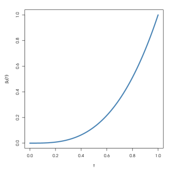
(a) Regression parameter $\beta_{0}$.

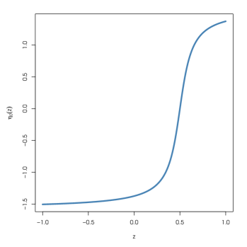
(b) Nonparametric component $\eta_{0}$.

Figure 1: True parameters.

We compared three estimators: the classical procedure based on least squares (ls), the $M$-estimators proposed by Huang et al. (2015) (m), and the $MM$-estimators (mm) from Section 2.1. Since the true function $\eta_{0}$ is monotone, we also included the modification, $\widehat{\eta}_{\mbox{\scriptsize\sc mod}}$, based on Neumeyer (2007). As in Huang et al. (2015), $M$-estimators were computed using a Huber function with tuning constant $1.345$ and no scale estimator. For the $MM$-estimators we used a bounded $\rho-$function $\rho_{0}$ to compute the initial $S$-estimators and residual scale in (4) and also a bounded $\rho_{1}$ for the $M$-step (6). For $j=0,1$, we choose $\rho_{j}=\rho_{\,\mbox{\scriptsize\sc tuk},\,c_{j}}$, the bisquare function, with tuning constants $c_{0}=1.54764$ ($b=1/2$) and $c_{1}=3.444$. All calculations were performed in R. The code and scripts reproducing the examples in this paper are publicly available on-line at https://github.com/msalibian/RobustFPLM.

For each setting we generated $n_{R}=500$ samples of size $n=300$ and used cubic splines with equally spaced knots. For the robust $MM$-estimators we selected the size of the spline bases ($p_{1}=k_{n,\beta}$ and $p_{2}=k_{n,\eta}$) by minimizing $RBIC(p_{1},p_{2})$ in equation (8) over the 2-dimensional grid $4\leq p_{1},p_{2}\leq 13$. For the least squares estimator we used the standard BIC criterion, and for the $M$-estimator we used the criterion proposed in Huang et al. (2015).

To evaluate the performance of each estimator we looked at their integrated squared bias and mean integrated squared error. These were computed on a grid of $M=100$ equally spaced points on $[0,1]$ and $[-1,1]$, for $\widehat{\beta}$ and $\widehat{\eta}$, respectively. More specifically, if $\widehat{\gamma}_{j}$ is the estimate of the function $\gamma$ obtained with the $j$-th sample ($1\leq j\leq n_{R}$), we compute

$$\mbox{Bias}^{2}(\widehat{\gamma})=\frac{1}{M}\sum_{s=1}^{M}\left(\frac{1}{n_{R}}\sum_{j=1}^{n_{R}}\widehat{\gamma}_{j}(t_{s})-\gamma(t_{s})\right)^{2}\,,$$

and

$$\mbox{MISE}(\widehat{\gamma})=\frac{1}{M}\sum_{s=1}^{M}\frac{1}{n_{R}}\sum_{j=1}^{n_{R}}\left(\widehat{\gamma}_{j}(t_{s})-\gamma(t_{s})\right)^{2}\,,$$

where $t_{1}\leq\dots\leq t_{M}$ are equispaced points on the domain ${\mathcal{I}}$ of $\gamma$. These are numerical approximations to

$$\int_{\mathcal{I}}\biggl{(}\frac{1}{n_{R}}\sum_{j=1}^{n_{R}}\widehat{\gamma}_{j}(t)-\gamma(t)\biggr{)}^{2}dt\,,$$

and

$$\frac{1}{n_{R}}\,\sum_{j=1}^{n_{R}}\int_{{\mathcal{I}}}\biggl{(}\widehat{\gamma}_{j}(t)-\gamma(t)\biggr{)}^{2}\,dt\,,$$

respectively. To alleviate the concern that $\mbox{Bias}^{2}$ and MISE may be heavily influenced by numerical errors at or near the boundaries of the grid, we follow He and Shi (1998) and also consider trimmed versions of the above computed without the $q$ first and last points on the grid:

$$\mbox{Bias}_{\mbox{\footnotesize\sc tr}}^{2}(\widehat{\gamma}) = \frac{1}{M-2q}\sum_{s=q+1}^{M-q}\left(\frac{1}{n_{R}}\sum_{j=1}^{n_{R}}\widehat{\gamma}_{j}(t_{s})-\gamma(t_{s})\right)^{2}\,,$$

$$\mbox{MISE}_{\mbox{\footnotesize\sc tr}}(\widehat{\gamma}) = \frac{1}{M-2q}\sum_{s=q+1}^{M-q}\frac{1}{n_{R}}\sum_{j=1}^{n_{R}}\left(\widehat{\gamma}_{j}(t_{s})-\gamma(t_{s})\right)^{2}\,,$$

We chose $q=[M\times 0.05]$ which uses the central 90% interior points in the grid. Table 1 reports the squared bias and MISE and their trimmed counterparts for samples without outliers. We note that the boundary effect is more pronounced for the estimators of $\beta_{0}$, but it is present for $\widehat{\eta}$ as well. Based on this observation, in what follows, we report the trimmed measures.

	$\widehat{\beta}$		$\widehat{\eta}$		$\widehat{\eta}_{\mbox{\scriptsize\sc mod}}$
	Bias2	MISE	Bias2	MISE	Bias2	MISE
ls	0.0126	0.1528	0.0197	0.0778	0.0221	0.0531
m	0.0123	0.1544	0.0248	0.0850	0.0261	0.0582
mm	0.0121	0.2039	0.0175	0.0871	0.0216	0.0593
	Bias${}^{2}_{\mbox{\footnotesize\sc tr}}$	MISE${}_{\mbox{\footnotesize\sc tr}}$	Bias${}^{2}_{\mbox{\footnotesize\sc tr}}$	MISE${}_{\mbox{\footnotesize\sc tr}}$	Bias${}^{2}_{\mbox{\footnotesize\sc tr}}$	MISE${}_{\mbox{\footnotesize\sc tr}}$
ls	0.0018	0.0865	0.0194	0.0615	0.0185	0.0442
m	0.0018	0.0869	0.0242	0.0680	0.0226	0.0493
mm	0.0017	0.1215	0.0173	0.0674	0.0171	0.0479

Table 1: Integrated squared bias and mean integrated squared errors over $n_{R}=500$ clean samples of size $n=300$. The top 3 rows report the Monte Carlo estimates of these measures using a grid of 100 equispaced points, and the bottom three correspond to their trimmed versions using the 90% inner grid points.

We considered two contamination scenarios. The first one contains outliers in the response variables and is expected to affect mainly the estimation of $\eta_{0}$. The second one includes high-leverage outliers in the functional explanatory variables, as in the Tecator example (see Section 5.2), which typically affect the estimation of the linear regression parameter $\beta_{0}$. Specifically, we constructed our samples as follows:

• Scenario $C_{1,\mu}$: here only the regression errors are contaminated in order to produce “vertical outliers”. Their distribution $G$ is given by $G(u)=0.9\,\Phi(u)+0.1\,\Phi\left((u-\mu)/0.5\right)$, with $\Phi$ the standard normal distribution function.

• Scenario $C_{2,\mu}$: in these settings we introduce high-leverage outliers by contaminating the functional covariates $X_{i}$ and the errors simultaneously. Outliers in the $X_{i}$’s are generated by perturbing the distribution of the second score in the Karhunen-Loève representation of the process. Specifically, we sample $v_{i}\sim Bi(1,0.10)$ and then:

  • if $v_{i}=0$, let $\epsilon_{i}^{(c)}=\epsilon_{i}$ and $X_{i}^{(c)}=X_{i}$;

  • if $v_{i}=1$, let $\epsilon_{i}^{(c)}\sim N(\mu,0.25)$ and $X_{i}^{(c)}=\sum_{j=1}^{50}\xi_{ij}^{(c)}\phi_{j}(t)$, with $\xi_{ij}^{(c)}\sim N(0,j^{-2})$ for $j\neq 2$ and $\xi_{i2}^{(c)}\sim N(\mu/2,0.25)$.

  The responses are generated as $y_{i}^{(c)}=\langle\beta_{0},X_{i}^{(c)}\rangle+\eta_{0}(z_{i})+\epsilon_{i}^{(c)}$.

Both contamination settings above depend on the parameter $\mu\in\mathbb{R}$. In this experiment we looked at the following values of $\mu$: 8, 10, 12, 14 and 16. They produce a range of contamination scenarios ranging from mild to severe. As an illustration of the type of outliers generated with the second setting above, Figure 2 shows 25 randomly chosen functional covariates $X_{i}(t)$, for one sample generated under $C_{0}$ (with no outliers) and one obtained under $C_{2,12}$.

(a) Some trajectories $X_{i}(t)$ under $C_{0}$.

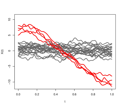
(b) Some trajectories $X_{i}(t)$ under $C_{2,12}$.

Figure 2: 25 trajectories $X_{i}(t)$ with and without contamination.

The plots in Figure 3 summarize the effect of the contamination scenarios for different values of $\mu$. Each plot corresponds to one contamination scenario and one parameter estimator. Within each panel, the solid, dashed and dotted lines correspond to the measures for the least squares, the $M$- and $MM$-estimators, respectively. There are two lines per estimation method: the one with triangles shows the trimmed MISE, and one with solid circles indicates the corresponding trimmed bias squared.

	$C_{1,\mu}$	$C_{2,\mu}$
$\widehat{\beta}$
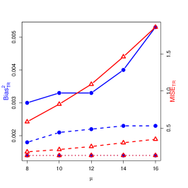
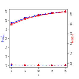
$\widehat{\eta}$
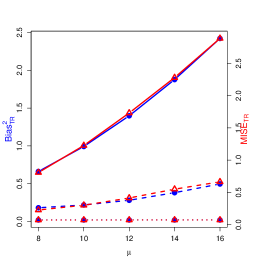
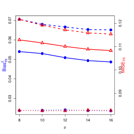
$\widehat{\eta}_{\mbox{\scriptsize\sc mod}}$

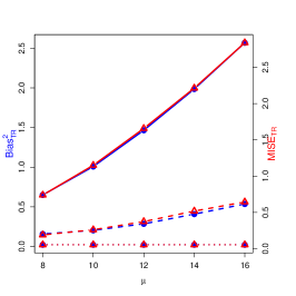
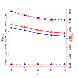
Figure 3: Plots of the trimmed squared bias and MISE of the estimators of $\beta_{0}$ and $\eta_{0}$ as a function of $\mu$ for both contamination scenarios: results for $C_{1,\mu}$ are in the first column of plots, while the second one contains those of $C_{2,\mu}$. The solid, dashed and dotted lines correspond to the least squares, the $M$- and $MM$-estimators, respectively. The squared bias is indicated with circles, and the MISE with triangles.

In order to also explore visually the performance of these estimators, Figures 4 to 6 contain functional boxplots (Sun and Genton, 2011) for the $n_{R}=500$ realizations of the different estimators for $\beta_{0}$ and $\eta_{0}$ under three contamination settings. As in standard boxplots, the central box of these functional boxplots represents the 50% inner band of curves, the solid black line indicates the central (deepest) function and the dotted red lines indicate outlying curves (in this case: outlying estimates $\widehat{\beta}_{j}$ or $\widehat{\eta}_{j}$ for some $1\leq j\leq n_{R}$). We also indicate the target (true) functions $\beta_{0}$ and $\eta_{0}$ with a dark green dashed line. To avoid boundary effects, we show here the different estimates $\widehat{\beta}_{j}$ or $\widehat{\eta}_{j}$ evaluated on the interior points of a grid of 100 equispaced points. In addition, to facilitate comparisons between contamination cases and estimation methods, the scales of the vertical axes are the same for all panels within each Figure.

	$\widehat{\beta}_{\mbox{\footnotesize\sc ls}}$	$\widehat{\beta}_{\mbox{\footnotesize\sc m}}$	$\widehat{\beta}_{\mbox{\footnotesize\sc m}\mbox{\footnotesize\sc m}}$
$C_{0}$
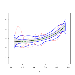
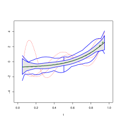
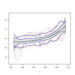
$C_{1,12}$
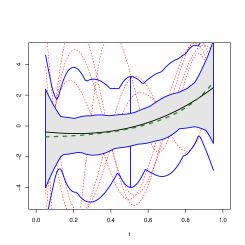
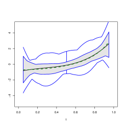
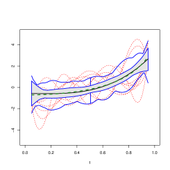
$C_{2,12}$

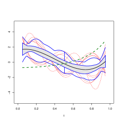
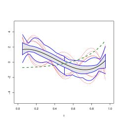
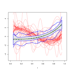
Figure 4: Functional boxplot of the estimators for $\beta_{0}$. The true function is shown with a green dashed line, while the black solid one is the central curve of the $n_{R}=500$ estimates $\widehat{\beta}$. Columns correspond to estimation methods while rows to three contaminations settings.

	$\widehat{\eta}_{\mbox{\footnotesize\sc ls}}$	$\widehat{\eta}_{\mbox{\footnotesize\sc m}}$	$\widehat{\eta}_{\mbox{\footnotesize\sc m}\mbox{\footnotesize\sc m}}$
$C_{0}$
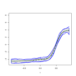
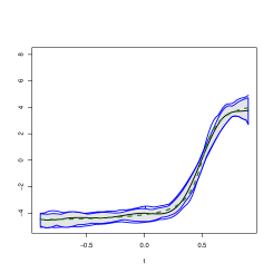
$C_{1,12}$
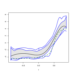
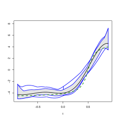
$C_{2,12}$

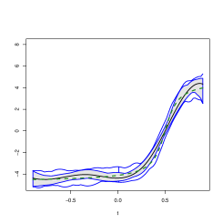
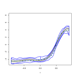
Figure 5: Functional boxplot of the estimators for $\eta_{0}$. The true function is shown with a green dashed line, while the black solid one is the central curve of the $n_{R}=500$ estimates $\widehat{\beta}$. Columns correspond to estimation methods while rows to three contaminations settings.

	$\widehat{\eta}_{\mbox{\footnotesize\sc ls},\mbox{\scriptsize\sc mod}}$	$\widehat{\eta}_{\mbox{\footnotesize\sc m},\mbox{\scriptsize\sc mod}}$	$\widehat{\eta}_{\mbox{\footnotesize\sc m}\mbox{\footnotesize\sc m},\mbox{\scriptsize\sc mod}}$
$C_{0}$
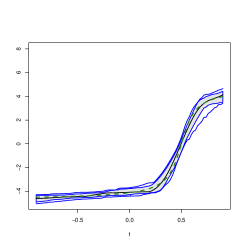
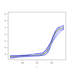
$C_{1,12}$
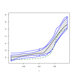
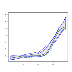
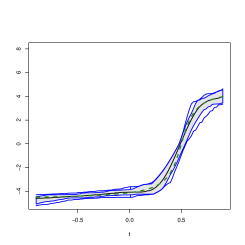
$C_{2,12}$

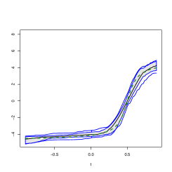
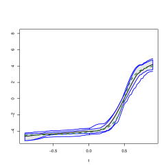
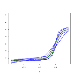
Figure 6: Functional boxplot of the monotone estimators for $\eta_{0}$. The true function is shown with a green dashed line, while the black solid one is the central curve of the $n_{R}=500$ estimates $\widehat{\beta}$. Columns correspond to estimation methods while rows to three contaminations settings.

As expected, when the data do not contain outliers, all estimators behave similarly to each other (see Table 1). When estimating the regression coefficient $\beta_{0}$, the less efficient robust $MM$-estimator naturally results in higher MISE’s. However, this efficiency loss is much smaller for the estimators of $\eta_{0}$. The serious damage caused to the least squares estimators by a small proportion of outliers (10%) can be seen clearly in Figure 3 (solid lines). The integrated squared bias and the MISE of the least squares estimators of $\beta_{0}$ and $\eta_{0}$ are consistently much higher than those of the robust $MM$-estimators. The ways in which the different oultiers affect the classical estimators for $\beta_{0}$ can be seen in Figure 4. Note that under $C_{1,12}$ the classical $\widehat{\beta}$ becomes highly variable, but mostly retains the same shape of the true $\beta_{0}$, which lies within the central box. However, with high-leverage outliers (as in $C_{2,12}$) the estimator becomes completely uninformative, and does not reflect the shape of the true regression coefficient $\beta_{0}$. The effect of outliers on the classical estimator for $\eta_{0}$ can be seen in Figure 5 (and Figure 6 for its monotone modification). We see that vertical outliers cause a vertical bias in the least squares estimator $\widehat{\eta}$, so that the central region of the functional boxplot fails to contain the true function $\eta_{0}$ for much of its domain. As expected, the effect of high-leverage outliers on $\widehat{\eta}$ is less marked, but certain upwards bias is apparent.

It is interesting to note that the $M$-estimators behave similarly to the classical ones. Vertical outliers result in more variable functional regression $M$-estimators $\widehat{\beta}$, although this increase is less pronounced than what we saw for the least squares estimators. High-leverage outliers are very damaging to these estimators. In particular, note from Figure 3 that in this case their integrated squared bias and MISE for $\widehat{\beta}$ are almost the same as those for the least squares estimator. We can also see this in Figure 4 where the $M$-estimators do not resemble the true function at all. Similar conclusions hold for the $M$-estimators for $\eta_{0}$. Vertical outliers produce an upward shift on the $\widehat{\eta}$’s, and a slight increase in variability, although this is less pronounced than what happened with classical estimators. The behaviour of the $M$-estimator $\widehat{\eta}$ with high-leverage outliers is similar to that of the least squares estimators, although notably their integrated squared bias and MISE is worse than those of the least squares estimators (Figure 3).

In contrast, the $MM$-estimators display a remarkably stable behaviour across contamination settings. Their bias and MISE curves in Figure 3 show that the $MM$-estimators for $\beta_{0}$ and $\eta_{0}$ are highly robust against both types of contamination scenarios considered here. If we look at the behaviour of these estimators in Figure 4 we note that the central box and the “whiskers” for the $MM$-estimators remain almost constant in all three simulation scenarios (clean data, vertical outliers and high-leverage outliers), in sharp constrast to what happens to the other estimators considered here. The number of affected $MM$ replicates for $\widehat{\beta}$ is higher for $C_{2,12}$ than it is for $C_{1,12}$, but even in the former case this happened for only 45 of the 500 $\widehat{\beta}$’s. We expect some effect on the estimators under this type of particularly damaging contamination, and we note that the robust proposal is the only one that can resist it in the vast majority of samples. The results in Figure 5 tell the same story, but less strickingly so. The $MM$-estimators for $\eta_{0}$ are almost unaffected by the different types of outliers, and the functional boxplots remain very similar to each other.

	$\widehat{\beta}$		$\widehat{\eta}$		$\widehat{\eta}_{\mbox{\scriptsize\sc mod}}$
Max over $C_{1,\mu}$	Bias${}^{2}_{\mbox{\footnotesize\sc tr}}$	MISE${}_{\mbox{\footnotesize\sc tr}}$	Bias${}^{2}_{\mbox{\footnotesize\sc tr}}$	MISE${}_{\mbox{\footnotesize\sc tr}}$	Bias${}^{2}_{\mbox{\footnotesize\sc tr}}$	MISE${}_{\mbox{\footnotesize\sc tr}}$
cl	0.0053	1.8616	2.4201	2.8861	2.5686	2.8384
m	0.0023	0.3499	0.4974	0.6651	0.5350	0.6438
mm	0.0014	0.1317	0.0218	0.0739	0.0209	0.0529
Max over $C_{2,\mu}$	Bias${}^{2}_{\mbox{\footnotesize\sc tr}}$	MISE${}_{\mbox{\footnotesize\sc tr}}$	Bias${}^{2}_{\mbox{\footnotesize\sc tr}}$	MISE${}_{\mbox{\footnotesize\sc tr}}$	Bias${}^{2}_{\mbox{\footnotesize\sc tr}}$	MISE${}_{\mbox{\footnotesize\sc tr}}$
cl	2.9685	3.1119	0.0540	0.1129	0.0474	0.0829
m	2.9891	3.1318	0.0705	0.1217	0.0583	0.0903
mm	0.0229	0.4341	0.0242	0.0828	0.0236	0.0607

Table 2: Values of the trimmed summary measures for the worst contamination settings under each scenario.

Table 2 reports the maximum values of Bias${}^{2}_{\mbox{\footnotesize\sc tr}}$ and MISE${}_{\mbox{\footnotesize\sc tr}}$ over $\mu$ for the two contamination settings $C_{1,\mu}$ and $C_{2,\mu}$. Regarding the behaviour of the estimators of the functional regression parameter $\beta_{0}$, high-leverage outliers ($C_{2,\mu}$) are more damaging for the classical and $M$-estimators than “vertical” ones ($C_{1,\mu}$). The increase in square bias shows that the estimation is completely distorted for these estimators. Note that the trimmed squared bias increases more than 1000 times and the MISE${}_{\mbox{\footnotesize\sc tr}}$ more than 30 times with respect to those reported in Table 1. In contrast, the classical estimator of $\eta_{0}$ is only slightly affected by $C_{2,\mu}$, since both the MISE${}_{\mbox{\footnotesize\sc tr}}$ are increased by a factor of at most 2.5 with respect to the ones obtained for clean samples. Vertical outliers, however, produce increases of more than $40$ times when $\mu=16$ where the maximum is attained (see Figure 3). Even though the $M$-estimators of Huang et al. (2015) are affected by both contaminations, they deteriorate less than the classical ones. In particular, when estimating $\eta_{0}$, the $M$-estimator at least triples the $\mathop{\rm MISE}_{\mbox{\footnotesize\sc tr}}$ under $C_{1,\mu}$ with respect to that obtained for clean samples (the worst effect is observed when $\mu=16$, reaching 10 times the value under $C_{0}$). Finally, the $MM$-estimators are quite stable under the considered contaminations. In particular, under $C_{1,\mu}$ the values of Bias${}^{2}_{\mbox{\footnotesize\sc tr}}$of $\widehat{\eta}_{\mbox{\footnotesize\sc m}}$ are between 8 and 20 times larger than those of $\widehat{\eta}_{\mbox{\footnotesize\sc m}\mbox{\footnotesize\sc m}}$, even for their monotone counterparts (see Figure 3), while the increase of the $\mathop{\rm MISE}_{\mbox{\footnotesize\sc tr}}$ of $\widehat{\eta}_{\mbox{\footnotesize\sc m}}$ varies between 3 and 9. Regarding the performance of the estimators of $\beta_{0}$, under $C_{1,\mu}$, the differences between the $MM$-estimators and the $M$-estimators are less pronounced than those between the $MM$- and the classical one. Under $C_{2,\mu}$, the worst $\mathop{\rm MISE}_{\mbox{\footnotesize\sc tr}}$ of $\widehat{\beta}_{\mbox{\footnotesize\sc m}\mbox{\footnotesize\sc m}}$ is multiplied less than 5 times with respect to that obtained under $C_{0}$. However, it is still only a sixth of the $\mathop{\rm MISE}_{\mbox{\footnotesize\sc tr}}$ for the classical and $M$-estimator, which suffer from a huge bias. In all cases, the $\mathop{\rm MISE}_{\mbox{\footnotesize\sc tr}}$ of $\widehat{\eta}_{\mbox{\scriptsize\sc mod}}$ is smaller than that of $\widehat{\eta}$.

5 Real data examples

5.1 German electricity prices

In our first example we look at the relationship between hourly electricity prices and the overall load of the German energy system. As discussed in Liebl (2013), such analysis needs to consider that eolic energy prices in this type of markets follow a different price regime. The data consist of hourly electricity prices in Germany between 1 January 2006 and 30 September 2008, as traded at the Leipzig European Energy Exchange, German electricity demand (as reported by the European Network of Transmission System Operators for Electricity), and the amount of eolic energy in the system (taken from the EEX Transparency Platform). The data set is available from the on-line supplementary materials of Liebl (2013). Weekends, holidays and other non-working days were removed from the dataset. Our model is

$$y=\langle X,\beta_{0}\rangle+\eta_{0}(z)+\sigma_{0}\epsilon\,,$$ (11)

where $y$ is the daily average hourly energy demand, $X$ is the curve of energy prices (as a function of time) observed hourly, and $z$ is the mean hourly amount of wind-generated electricity in the system for that day. As usual, $\epsilon$ is a random variable centered at zero, and independent from $X$ and $z$. The shape of the function $\beta_{0}$ can be used to identify times of the day when hourly prices are informative regarding the overall system demand.

In addition to our proposed robust $MM$-estimators, we also computed the classical least squares and the $M$-estimators of Huang et al.​​ (2015). The robust $MM$-estimators were calculated using the same $\rho$-functions as in our simulation study and we selected the size of the splines bases with the $RBIC$ criterion (8). Following Huang et al.​​ (2015), the $M$-estimator was computed using a Huber function with tuning constant equal to $1.345$ and no scale estimator.

The estimators for $\beta_{0}$ and $\eta_{0}$ are shown in Figures 7(a) and 7(b), respectively. Solid black lines are used for the $MM$-estimator, and solid gray ones for the least squares one. The $M$-estimators were indistinguishable from the classical ones and so we did not include them in these plots. Comparing the $MM$ and classical estimators for $\beta_{0}$, we note that the robust fit identifies two “peak” times (around 4am and 8pm) and two “slump” times around 3pm and 11pm, where prices have a larger (in magnitude) association with the daily average load in the system. However, the least squares fit appears to not include the early afternoon prices as important (note that the magnitude of the function $\hat{\beta}_{0}$ is smaller than that of the robust estimator between 2pm and 8pm). On the other hand, although the estimators for $\eta$ are slightly different, their shapes are rather consistent with each other.

We next identified potential outliers in the data by using a boxplot of the residuals from the robust $MM$-fit. The dashed lines in Figures 7(a) and 7(b) correspond to the classical fit computed without these possible atypical observations. We note that the classical estimators computed without these potential outliers are very close to the robust ones. In other words, the robust estimator behaves similarly to the classical one if one were able to manually remove suspected outliers.

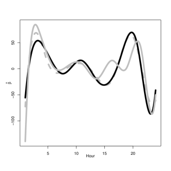
(a) Estimates of $\beta_{0}$

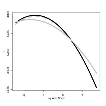
(b) Estimates of $\eta_{0}$

Figure 7: German Electricity: Estimates of $\beta_{0}$ and $\eta_{0}$. The black line corresponds to the $MM$-fit, while the solid and dashed gray ones correspond to the least squares computed with the whole training set and without the outliers, respectively. The $M$-estimators were almost identical to the least squares ones, and not included in this plot.

5.2 Tecator

The Tecator data set was analysed in Ferraty and Vieu (2006), Aneiros-Pérez and Vieu (2006), Shang (2014) and Huang et al. (2015), and it is available in the package fda.usc (Febrero-Bande and Oviedo de la Fuente, 2012). See also http://lib.stat.cmu.edu/datasets/tecator. These data contain measurements taken on samples from finely chopped meat with different percentages of fat, protein and moisture content. Each observation consists of a spectrometric curve, ${\mathcal{X}}_{i}$, which corresponds to the absorbance measured on an equally spaced grid of 100 wavelengths between 850 and 1050nm. The goal of the analysis is to predict the fat content ($y$) using the spectrometric curve (${\mathcal{X}}$) and the variables water ($v$) and protein contents ($z$).

Huang et al. (2015) compared several models in terms of their predictive properties. They used the second derivative $X$ of the spectrometric curve as the functional covariate, which enters the model linearly, while the variables $(z,v)$ appear either through an additive non-parametric component or a varying coefficient model

$$y=\gamma_{0}+\langle X,\beta_{0}\rangle+v\,\eta_{0}(z)+\sigma_{0}\epsilon\,,$$ (12)

where $\gamma_{0}\in\mathbb{R}$ and $\eta_{0}$ is a smooth function of $z$.

Following Aneiros-Pérez and Vieu (2006), the sample was divided into a training set (corresponding to the first $155$ observations) and a testing one with the remaining $60$ data points. As in Section 4, the $M$-estimators of Huang et al. (2015) were computed using a Huber function with tuning constant $1.345$ and no scale estimator. The robust $MM$-estimators were calculated using the same $\rho-$functions as in our simulation study and we selected the size of the splines bases with the $RBIC$ criterion (8). To compare the predictions obtained with the different estimators we computed the mean and median square prediction errors on the test set:

$$MSPE=\frac{1}{n_{{\mathcal{J}}}}\sum_{j\in{\mathcal{J}}}\frac{(y_{i}-\widehat{y}_{i})^{2}}{s^{2}_{{\mathcal{J}}}}\quad\mbox{and}\quad MedSPE=\frac{\mbox{median}(y_{i}-\widehat{y}_{i})^{2}}{s^{2}_{{\mathcal{J}}}}\,,$$

where ${\mathcal{J}}$ contains the indices of the observations in the test set, $n_{{\mathcal{J}}}$ denotes its size, and $s_{{\mathcal{J}}}=\mathop{\mbox{\sc mad}}_{j\in{\mathcal{J}}}(y_{j})$.

The first three columns and two rows of Table 3 report the mean and median square prediction errors for the classical, $M$ and $MM$-estimators. Although the least squares and $M$ fits have lower mean squared prediction errors than that of the robust $MM$ one, their larger median suggests that most prediction errors may in fact be smaller for the robust estimator, but that a few outliers may be present in the test set.

	ls	m	mm	ls${}^{-\;out}$
$1000\times MSPE$	2.52	2.44	4.56	4.83
$1000\times MedSPE$	0.95	0.85	0.65	0.78
$1000\times MSPE_{\mbox{\scriptsize\sc clean}}$	1.47	1.42	1.33	1.40

Table 3: Mean and median square prediction errors of the classical, $M$ and $MM$-estimators labelled ls, m and mm, respectively.

To evaluate the ability of the procedure to predict non-outlying observations, we also computed the mean squared prediction errors over non-outlying points in the test set:

$$MSPE_{\mbox{\scriptsize\sc clean}}=\frac{1}{n_{{\mathcal{J}}}-\sum_{i\in{\mathcal{J}}}\gamma_{i}}\;\sum_{j\in{\mathcal{J}}}(1-\gamma_{j})\,\frac{(y_{j}-\widehat{y}_{j})^{2}}{s_{{\mathcal{J}}}^{2}}\,,$$

where $\gamma_{i}=1$ if the $i$-th observation was flagged as atypical, and 0 otherwise. To identify potential outliers in the data we used the boxplots of the residuals from the fits obtained using the $MM$-procedure both for the training and testing sets. The mean squared prediction errors of both estimators using the non-outlying points in the test set ($MSPE_{\mbox{\scriptsize\sc clean}}$) are reported in the last row of Table 3. Note that now the $MSPE_{\mbox{\scriptsize\sc clean}}$ for the $MM$-estimators is smaller than those of the least squares and $M$-estimators. The fourth column ($\textsc{ls}^{-out}$) of that table displays the results obtained with the classical estimator when it was computed without the 13 potential outliers in the training set. Since the $M$-estimators of Huang et al. (2015) behaved very similarly to the classical ones from now on, we only comment the results obtained when using the least squares and the $MM$-estimators.

As in the German Electricity example, we note that the classical procedure trained after eliminating potential atypical observations gives very similar results to those obtained with the $MM$-estimator. The black and gray solid lines in Figures 8(a) and 8(b) show the estimators $\widehat{\eta}$ and $\widehat{\beta}$ obtained using the classical and robust estimators, respectively. On both panels we also overlay (in dashed gray lines) the corresponding least squares estimates computed on the “cleaned” training set. In both cases it is clear that the classical estimators are seriously affected by the atypical training points, while the robust estimator provides estimates similar to those that are obtained with the classical methods after removing possible outliers.

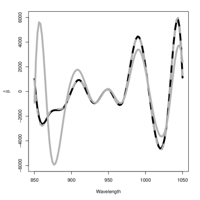
(a) Estimates of $\beta_{0}$

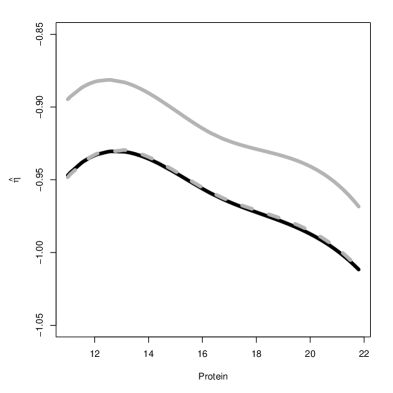
(b) Estimates of $\eta_{0}$

Figure 8: Tecator: Estimates of $\beta_{0}$ and $\eta_{0}$. The black line corresponds to the $MM$-fit, while the solid and dashed gray ones correspond to the least squares computed with the whole training set and without the outliers, respectively.

6 Conclusion

In this paper we propose robust estimators based on $B$-splines for semi-functional linear regression models. Our estimators are robust against outliers in the response variable, and also in the functional explanatory variables. Furthermore, we propose a robust $BIC$-type criterion to select the optimal dimension of the splines bases that works very well in practice. We prove that the estimators are strongly consistent under standard regularity conditions, and show how they can be extended rather straightforwardly to other semiparametric models with functional covariates that enter the model linearly. A simulation study shows that our proposed estimators have good robustness and finite-sample statistical properties.

We apply our method to two real data sets and confirm that the robust $MM$-estimators remain reliable even when the training set contains atypical observations in the functional explanatory variables. Moreover, the residuals obtained from the robust fit provide a natural way to identify potential atypical observations.

7 Acknowledgements.

The authors would like to thank Professor Ioannis Kalogridis for his careful reading of earlier versions of this manuscript and for pointing out a mistake in the proof of Theorem 3.2 which has been corrected in the current version. This research was partially supported by Universidad de Buenos Aires [Grant 20020170100022ba] and anpcyt [Grant pict 2018-00740] at Argentina (Graciela Boente and Pablo Vena), the Ministry of Economy, Industry and Competitiveness, Spain (MINECO/AEI/FEDER, UE) [Grant MTM2016-76969P] (Graciela Boente) and by the Natural Sciences and Engineering Research Council of Canada [Discovery Grant RGPIN-2016-04288] (M. Salibián Barrera).

A Appendix

A.1 Proofs of Proposition 3.1 and Theorem 3.1

In what follows, ${\mathcal{V}}$ stands for a neighbourhood of $\sigma_{0}$ with closure $\overline{{\mathcal{V}}}$ strictly included in $(0,\infty)$. Furthermore, recall that we have denoted ${\mathcal{L}}_{r}={\mathcal{L}}_{r}([0,1])$, $r\geq 1$, the space of functions whose $r-$th derivative satisfies a Lipschitz condition in $[0,1]$:

$${\mathcal{L}}_{r}([0,1])=\Bigl{\{}g\in C^{r}\left([0,1]\right):\big{\|}g^{(j)}\big{\|}_{\infty}<\infty,\;0\leq j\leq r\,,\mbox{ and }\,\sup_{z_{1}\neq z_{2}}\frac{\big{|}g^{(r)}(z_{1})-g^{(r)}(z_{2})\big{|}}{|z_{1}-z_{2}|}<\infty\Bigr{\}}\,.$$

We use the following norm

$$\|f\|_{{\mathcal{L}}_{r}}=\max_{1\leq j\leq r}\big{\|}f^{(j)}\big{\|}_{\infty}+\sup_{x\neq y,x,y\in(0,1)}\frac{\big{|}f^{(r)}(x)-f^{(r)}(y)\big{|}}{|x-y|}\,,$$

where $f^{(j)}$ stands for the $j$-th derivative of $f$. The unit ball in ${\mathcal{L}}_{r}$ will be denoted as ${\mathcal{V}}_{1}^{(r)}=\{f\in{\mathcal{L}}^{r}([0,1]):\|f\|_{{\mathcal{L}}_{r}}\leq 1\}$.

We begin by stating some Lemmas that will be used in the proofs of Proposition 3.1 and Theorem 3.1. Lemma A.1.1 entails that the functional related to the considered estimators are indeed Fisher–consistent, which is a condition needed to ensure that we are estimating the target quantities.

Lemma A.1.1. Assume that C1 holds and let $\rho$ be a function satisfying R1. Then, we have that, for any $\sigma>0$,

• $M(\beta,\eta,\sigma)\geq M(\beta_{0},\eta_{0},\sigma)$, where

  $$M(\beta,\eta,\sigma)=\mathbb{E}\,\rho\left(\frac{y-\langle X,\beta\rangle-\eta(z)}{\sigma}\right)\,.$$

• If in addition C2 holds, $(\beta_{0},\eta_{0})$ is the unique minimizer of $M(\beta,\eta,\sigma)$.

Proof. Lemma 3.1 of Yohai (1987) together with R1 and the fact that $\widetilde{\epsilon}=\epsilon\sigma_{0}/\sigma$ satisfy assumption C1 imply that for all $a\neq 0$,

$$\mathbb{E}\left[\rho\left(\epsilon\frac{\sigma_{0}}{\sigma}-a\right)\right]>\mathbb{E}\left[\rho\left(\epsilon\frac{\sigma_{0}}{\sigma}\right)\right]\,,$$ (A.1)

and a) follows immediately.

To derive b), denote as ${\mathcal{A}}_{0}\,=\,\left\{(X,z):\Phi(X,z)=\langle X,\beta-\beta_{0}\rangle+\eta(z)-\eta_{0}(z)=0\right\}$ and $a(X,z)=\Phi(X,z)/\sigma$. Then, we have that

$$M(\beta,\eta,\sigma) = \mathbb{E}\rho\left(\frac{\epsilon\sigma_{0}-\Phi(X,z)}{\sigma}\right)=\mathbb{E}\rho\left(\epsilon\frac{\sigma_{0}}{\sigma}-\frac{\Phi(X,z)}{\sigma}\right)$$

$$= \mathbb{E}\left\{\rho\left(\epsilon\frac{\sigma_{0}}{\sigma}\right)\mathbb{I}_{{\mathcal{A}}_{0}}(X,z)\right\}\,+\,\mathbb{E}\left\{\mathbb{E}\left[\rho\left(\epsilon\frac{\sigma_{0}}{\sigma}-a(X,z)\right)|(X,z)\right]\mathbb{I}_{{\mathcal{A}}_{0}^{c}}(X,z)\right\}$$

$$= \mathbb{E}\left(\rho\left(\epsilon\frac{\sigma_{0}}{\sigma}\right)\right)\mathbb{E}\left\{\mathbb{I}_{{\mathcal{A}}_{0}}(X,z)\right\}\,+\,\mathbb{E}\left\{\mathbb{E}\left[\rho\left(\epsilon\frac{\sigma_{0}}{\sigma}-a(X,z)\right)|(X,z)\right]\mathbb{I}_{{\mathcal{A}}_{0}^{c}}(X,z)\right\}\,.$$

Note that (A.1) entails that, for any $(X,z)\notin{\mathcal{A}}_{0}$,

$$\mathbb{E}\left[\rho\left(\epsilon\frac{\sigma_{0}}{\sigma}-a(X,z)\right)|(X,z)=(X_{0},z_{0})\right] = \mathbb{E}\left[\rho\left(\epsilon\frac{\sigma_{0}}{\sigma}-a(X_{0},z_{0})\right)|(X,z)=(X_{0},z_{0})\right]$$

$$= \mathbb{E}\left[\rho\left(\epsilon\frac{\sigma_{0}}{\sigma}-a(X_{0},z_{0})\right)\right]>\mathbb{E}\left[\rho\left(\epsilon\frac{\sigma_{0}}{\sigma}\right)\right]\,,$$

where the last equality follows from the fact that the errors are independent of the covariates. Thus, using that $\mathbb{P}({\mathcal{A}}_{0}^{c})>0$ from C2, we get

$$M(\beta,\eta,\sigma) =\mathbb{E}\rho\left(\epsilon\frac{\sigma_{0}}{\sigma}\right)\,\mathbb{P}\left({{\mathcal{A}}_{0}}\right)\,+\,\mathbb{E}\left\{\mathbb{E}\left[\rho\left(\epsilon\frac{\sigma_{0}}{\sigma}-a(X,z)\right)|(X,z)\right]\mathbb{I}_{{\mathcal{A}}_{0}^{c}}(X,z)\right\}$$

$$>\mathbb{E}\rho\left(\epsilon\frac{\sigma_{0}}{\sigma}\right)\,\mathbb{P}\left({{\mathcal{A}}_{0}}\right)\,+\,\mathbb{E}\left\{\mathbb{E}\left[\rho\left(\epsilon\frac{\sigma_{0}}{\sigma}\right)\right]\mathbb{I}_{{\mathcal{A}}_{0}^{c}}(X,z)\right\}$$

$$>\mathbb{E}\rho\left(\epsilon\frac{\sigma_{0}}{\sigma}\right)\,\mathbb{P}\left({{\mathcal{A}}_{0}}\right)+\mathbb{E}\rho\left(\epsilon\frac{\sigma_{0}}{\sigma}\right)\,\mathbb{P}\left({{\mathcal{A}}_{0}^{c}}\right)$$

$$>\mathbb{E}\left(\rho\left(\epsilon\frac{\sigma_{0}}{\sigma}\right)\right)=M(\beta_{0},\eta_{0},\sigma)\,.\;\qed$$

Let ${\mathcal{M}}_{p_{s}}^{(s)}$, $s=1,2$, denote the linear spaces spanned by the $B$-splines bases of size $p_{1}$ and $p_{2}$:

$${\mathcal{M}}_{p_{s}}^{(s)}=\left\{\sum_{j=1}^{p_{s}}b_{j}\,B_{j}^{(s)}(t)\,,\,\mathbf{b}\in\mathbb{R}^{p_{s}}\right\}\quad s=1,2\,.$$

Recall that $p_{1}$ and $p_{2}$ increase with the sample size $n$. The Lemmas below will be useful to derive consistency of the proposed estimators. In particular, the next lemma shows that

$$M_{n}(\beta,\eta,\sigma)=\frac{1}{n}\sum_{i=1}^{n}\ \rho\left(\frac{y_{i}-\langle X_{i},\beta\rangle-\eta(z_{i})}{\sigma}\right)\,,$$

converges to $M(\beta,\eta,\sigma)$ with probability one, uniformly over $\sigma>0$ and ${\mathcal{M}}_{p_{1}}^{(1)}\times{\mathcal{M}}_{p_{2}}^{(2)}$.

Lemma A.1.2. Let $\rho$ be a bounded function satisfying R1 and R2 and assume that C4 holds. Let $p_{1}=k_{n,\beta}$ and $p_{2}=k_{n,\eta}$. Then, we have that,

• $\sup_{\sigma>0,\beta\in{\mathcal{M}}_{p_{1}}^{(1)},\eta\in{\mathcal{M}}_{p_{2}}^{(2)}}\left|M_{n}(\beta,\eta,\sigma)-M(\beta,\eta,\sigma)\right|\buildrel a.s.\over{\longrightarrow}0$.

• Furthermore,

  $$\sup_{\sigma>0,\beta\in{\mathcal{M}}_{p_{1}}^{(1)},\eta\in{\mathcal{M}}_{p_{2}}^{(2)}}\left|\frac{1}{n-p_{1}-p_{2}}\sum_{i=1}^{n}\left[\rho\left(\frac{y_{i}-\langle X_{i},\beta\rangle-\eta(z_{i})}{\sigma}\right)-M(\beta,\eta,\sigma)\right]\right|\buildrel a.s.\over{\longrightarrow}0\,.$$

Proof. b) follows immediately from a) noting that $n/(n-p_{1}-p_{2})\to 1$.

To prove (a) we need to introduce some notation. For any measure $\mathbb{Q}$, $N(\epsilon,{\mathcal{F}}_{n},L_{s}(\mathbb{Q}))$ and $N_{[\;]}(\epsilon,{\mathcal{F}}_{n},L_{s}(\mathbb{Q}))$ stand for the covering and bracketing numbers of the class ${\mathcal{F}}_{n}$ with respect to the distance in $L_{s}(\mathbb{Q})$, as defined, for instance, in van der Vaart and Wellner (1996).

Recall that we have denoted as $\mathbf{B}(z)=(B_{1}^{(2)}(z),\dots,B_{p_{2}}^{(2)}(z))^{\mbox{\footnotesize\sc t}}$ and $\mathbf{x}=(\langle X,B_{1}^{(1)}\rangle,\dots,$ $\langle X,B_{p_{1}}^{(1)}\rangle)^{\mbox{\footnotesize\sc t}}$ and define the class of functions

$${\mathcal{F}}_{n}=\{f(y,\mathbf{x},z)=\rho\left(\frac{y-\mathbf{b}^{\mbox{\footnotesize\sc t}}\mathbf{x}-\mathbf{a}^{\mbox{\footnotesize\sc t}}\mathbf{B}(z)}{\sigma}\right),\mathbf{b}\in\mathbb{R}^{p_{1}},\mathbf{a}\in\mathbb{R}^{p_{2}},\sigma>0\}\,,$$

To obtain a), first note that the boundedness of $\rho$ and R1, entails that the class ${\mathcal{F}}_{n}$ has envelope 1. Lemma S.2.1 in Boente et al. (2020) allows to bound, for any probability measure $\mathbb{Q}$, the covering number $N(2\epsilon;{\mathcal{F}}_{n};L_{1}(\mathbb{Q}))$ as

$$N(2\epsilon;{\mathcal{F}}_{n};L_{1}(\mathbb{Q}))\leq\left[Kq_{n}\;(16e)^{q_{n}}\left(\frac{1}{\epsilon}\right)^{q_{n}-1}\right]^{2}\,,$$ (A.2)

where $q_{n}=2(p_{1}+p_{2}+3)-1$. Hence, using that $\log(q_{n})/({p_{1}+p_{2}+3})<1$ and assuming without loss of generality that $K>1$, we get from (A.2) that

$$\log\left(N(2\,\epsilon,{\mathcal{F}}_{n},L_{1}(\mathbb{Q}))\right) \leq \log\left[Kq_{n}\;(16e)^{q_{n}}\left(\frac{1}{\epsilon}\right)^{q_{n}-1}\right]^{2}$$

$$\leq 2\left\{\log(K)+\log q_{n}\;+q_{n}\log(16e)+(q_{n}-1)\log\left(\frac{1}{\epsilon}\right)\right\}$$

$$\leq 2\left\{q_{n}\left[\log(K)+1+\log(16e)+\log\left(\frac{1}{\epsilon}\right)\right]\right\}$$

$$\leq C(p_{1}+p_{2})\log\left(\frac{1}{\epsilon}\right)\,,$$

for $\epsilon<\min((16e)^{-1},e^{-K})$ and some constant $C$. Thus, using that from C4 $p_{j}=O(n^{\nu})$ with $\nu<1$, we conclude that

$$\frac{1}{n}\log N(2\epsilon,{\mathcal{F}}_{n},L_{1}(P_{n})) \leq C\,\frac{p_{1}+p_{2}}{n}\,\log\left(\frac{1}{\epsilon}\right)\to 0\,,$$

which entails, (see, for instance, exercise 3.6 in van der Geer, 2000 with $b_{n}=2$), that

$$\sup_{\sigma>0,\beta\in{\mathcal{M}}_{p_{1}}^{(1)},\eta\in{\mathcal{M}}_{p_{2}}^{(2)}}\left|M_{n}(\beta,\eta,\sigma)-M(\beta,\eta,\sigma)\right|\buildrel a.s.\over{\longrightarrow}0\,,$$

concluding the proof. ∎

Lemma A.1.3. Let $\rho$ be a bounded function satisfying R1 and R2. Assume that C1 to C4 hold. Then, if in addition $\widehat{\sigma}\buildrel a.s.\over{\longrightarrow}\sigma_{0}$, we have that, $M(\widehat{\beta},\widehat{\eta},\sigma_{0})\buildrel a.s.\over{\longrightarrow}M(\beta_{0},\eta_{0},\sigma_{0})$.

Proof. Recall that $p_{1}$ and $p_{2}$ stand for $p_{1}=k_{n,\beta}$ and $p_{2}=k_{n,\eta}$ which are assumed to be of order $O(n^{\nu})$. Furthermore, we have denoted as $r_{i}(\beta_{\mathbf{b}},\eta_{\mathbf{a}})=y_{i}-\mathbf{b}^{\mbox{\footnotesize\sc t}}\mathbf{x}_{i}-\mathbf{a}^{\mbox{\footnotesize\sc t}}\mathbf{B}_{i}$, where $\mathbf{x}_{i}=(x_{i1},\dots,x_{ip_{1}})^{\mbox{\footnotesize\sc t}}$, $x_{ij}=\langle X_{i},B_{j}^{(1)}\rangle$ and $\mathbf{B}_{i}=(B_{1}^{(2)}(z_{i}),\dots,B_{p_{2}}^{(2)}(z_{i}))^{\mbox{\footnotesize\sc t}}$, while

$$M_{n}(\beta,\eta,\sigma) = \frac{1}{n}\sum_{i=1}^{n}\rho\left(\frac{y_{i}-\langle X_{i},\beta\rangle-\eta(z_{i})}{\sigma}\right)\,.$$

Lemma A.1.2 implies that

$$A_{n}=\sup_{\sigma>0,\beta\in{\mathcal{M}}_{p_{1}}^{(1)},\eta\in{\mathcal{M}}_{p_{2}}^{(2)}}\left|M_{n}(\beta,\eta,\sigma)-M(\beta,\eta,\sigma)\right|\buildrel a.s.\over{\longrightarrow}0\,.$$ (A.3)

On the other hand, Lemma A.1.1 entails that $M(\beta_{0},\eta_{0},\sigma)=\inf_{\beta,\eta}M(\beta,\eta,\sigma)$, for any $\sigma>0$, so

$$0\leq M(\widehat{\beta},\widehat{\eta},\sigma_{0})-M(\beta_{0},\eta_{0},\sigma_{0})=\sum_{i=1}^{3}A_{n,i}\,,$$

with

$$A_{n,1} = M(\widehat{\beta},\widehat{\eta},\widehat{\sigma})-M_{n}(\widehat{\beta},\widehat{\eta},\widehat{\sigma})\,,$$

$$A_{n,2} = M_{n}(\widehat{\beta},\widehat{\eta},\widehat{\sigma})-M(\beta_{0},\eta_{0},\sigma_{0})\,,$$

$$A_{n,3} = M(\widehat{\beta},\widehat{\eta},\sigma_{0})-M(\widehat{\beta},\widehat{\eta},\widehat{\sigma})\,.$$

Note that $|A_{n,1}|\leq A_{n}$, which together with (A.3) leads to $A_{n,1}\buildrel a.s.\over{\longrightarrow}0$. Using a Taylor’s expansion of order one and assumption R2, we get that

$$|A_{n,3}|\leq\|\zeta\|_{\infty}\frac{|\sigma_{0}-\widehat{\sigma}|}{\widehat{\xi}}\,,$$

where $\widehat{\xi}=\theta\sigma_{0}+(1-\theta)\widehat{\sigma}$ is an intermediate point, which together with the fact that $\widehat{\sigma}\buildrel a.s.\over{\longrightarrow}\sigma_{0}$ lead to $A_{n,3}\buildrel a.s.\over{\longrightarrow}0$.

We will now bound $A_{n,2}$. Using C3 and C4 and that $\ell\geq r+2$, we get from Corollary 6.21 in Schumaker (1981) that there exist $\widetilde{\beta}\in{\mathcal{M}}_{p_{1}}^{(1)}$ and $\widetilde{\eta}\in{\mathcal{M}}_{p_{2}}^{(2)}$ such that

$$\|\widetilde{\beta}-\beta_{0}\|_{\infty}=O(n^{-r\,\nu})\qquad\qquad\|\widetilde{\eta}-\eta_{0}\|_{\infty}=O(n^{-r\,\nu})\,.$$

Hence, using that $(\widehat{\beta},\widehat{\eta})$ minimize $M_{n}(\cdot,\cdot,\widehat{\sigma})$, we obtain that $A_{n,2}\leq M_{n}(\widetilde{\beta},\widetilde{\eta},\widehat{\sigma})-M(\beta_{0},\eta_{0},\sigma_{0})=\sum_{j=1}^{3}C_{n,j}$, where $C_{n,1}=M_{n}(\widetilde{\beta},\widetilde{\eta},\widehat{\sigma})-M(\widetilde{\beta},\widetilde{\eta},\widehat{\sigma})$, $C_{n,2}=M(\widetilde{\beta},\widetilde{\eta},\sigma_{0})-M(\beta_{0},\eta_{0},\sigma_{0})$ and $C_{n,3}=M(\widetilde{\beta},\widetilde{\eta},\widehat{\sigma})-M(\widetilde{\beta},\widetilde{\eta},\sigma_{0})$. Note that the strong consistency of $\widehat{\sigma}$ and the fact that $\widetilde{\beta}\in{\mathcal{M}}_{p_{1}}^{(1)}$ and $\widetilde{\eta}\in{\mathcal{M}}_{p_{2}}^{(2)}$ entail that $|C_{n,1}|$ can be bounded by $A_{n}$, so that $|C_{n,1}|\buildrel a.s.\over{\longrightarrow}0$. Arguing as above when bounding $A_{n,3}$, we conclude that $C_{n,3}\buildrel a.s.\over{\longrightarrow}0$. Finally, using that $\|\widetilde{\beta}-\beta_{0}\|_{\infty}+\|\widetilde{\eta}-\eta_{0}\|_{\infty}\to 0$ entail that for any $(y,X.z)$, $y-\langle X,\widetilde{\beta}\rangle+\widetilde{\eta}(z)\to y-\langle X,\beta_{0}\rangle+\eta_{0}(z)$, together with the continuity and boundedness of $\rho$ and the bounded convergence theorem leads to $C_{n,2}\to 0$. Hence, we get that

$$0\leq M(\widehat{\beta},\widehat{\eta},\sigma_{0})-M(\beta_{0},\eta_{0},\sigma_{0})\buildrel a.s.\over{\longrightarrow}0\,,$$

that is, $M(\widehat{\beta},\widehat{\eta},\sigma_{0})\buildrel a.s.\over{\longrightarrow}M(\beta_{0},\eta_{0},\sigma_{0})$, concluding the proof of a). Note that the fact that $A_{n,3}\buildrel a.s.\over{\longrightarrow}0$ entails also that $M(\widehat{\beta},\widehat{\eta},\widehat{\sigma})\buildrel a.s.\over{\longrightarrow}M(\beta_{0},\eta_{0},\sigma_{0})$. ∎

Lemma A.1.4. Let $\rho$ be a bounded function satisfying R1 and R2 and such that $M(\beta_{0},\eta_{0},\sigma_{0})=b_{\rho}<1$. Let $p_{1}=k_{n,\beta}$, $p_{2}=k_{n,\eta}$ and $(\widehat{\beta},\widehat{\eta})\in{\mathcal{M}}_{p_{1}}^{(1)}\times{\mathcal{M}}_{p_{2}}^{(2)}$ be such that $M(\widehat{\beta},\widehat{\eta},\sigma_{0})\buildrel a.s.\over{\longrightarrow}M(\beta_{0},\eta_{0},\sigma_{0})$. Assume that $\mathbb{E}\|X\|^{2}<\infty$ and that C3 and C5 hold with $c<1-b_{\rho}$. Then, we have that, there exists $L$ such that $\mathbb{P}(\cup_{m\in\mathbb{N}}\cap_{n\geq m}\|\widehat{\beta}-\beta_{0}\|_{{\mathcal{L}}_{1}}+\|\widehat{\eta}-\eta_{0}\|_{{\mathcal{L}}_{1}}\leq L)=1$.

Note that $M(\beta_{0},\eta_{0},\sigma_{0})\leq b<1$ whenever $\rho\leq\rho_{0}$, so if $c<1-b$ then $c<1-b_{\rho}$ and the condition $c<1-b$ was also a requirement in Yohai (1987).

Proof. Recall that ${\mathcal{V}}_{1}^{(1)}$ is a compact set for the topology of the norm $\|\cdot\|_{\infty}$, that is, as merged in ${\mathcal{C}}([0,1])$. Given $\delta>0$, define $K_{\delta}$ such that for any $K\geq K_{\delta}$,

$$\mathbb{P}(\|X\|\geq K)<\delta\,.$$ (A.4)

Let ${\mathcal{B}}=\{(\beta,\eta):\|\beta\|_{{\mathcal{L}}_{1}}+\|\eta\|_{{\mathcal{L}}_{1}}=1\}\subset{\mathcal{V}}_{1}^{(1)}\times{\mathcal{V}}_{1}^{(1)}$ and fix $\theta=(\beta,\eta)\in{\mathcal{B}}$. Let $\phi_{\theta}>0$ be a continuity point of the distribution of $|\langle X,\beta\rangle+\eta(z)|$ such that

$$\mathbb{P}\left(|\langle X,\beta\rangle+\eta(z)|<\phi_{\theta}\right)<c\,.$$

Then, if $\beta^{\star},\eta^{\star}\in{\mathcal{C}}([0,1])$ is such that $\max\left(\|\beta^{\star}-\beta\|_{\infty},\|\eta^{\star}-\eta\|_{\infty}\right)<\vartheta_{\theta}$, where $\vartheta_{\theta}=\phi_{\theta}/(2(K+1))$, we have that

$$\mathbb{P}\left(|\langle X,\beta^{\star}\rangle+\eta^{\star}(z)|\geq\frac{\phi_{\theta}}{2}\right)\geq\mathbb{P}\left(|\langle X,\beta\rangle+\eta(z)|\geq\phi_{\theta}\right)-\mathbb{P}\left(\vartheta_{\theta}(\|X\|+1)\geq\frac{\phi_{\theta}}{2}\right)\,=\,A(\theta)\,.$$

Hence, noting that $A(\theta)>1-c-\delta$, we conclude that

$$\inf_{\max\left(\|\beta^{\star}-\beta\|_{\infty},\|\eta^{\star}-\eta\|_{\infty}\right)<\vartheta_{\theta}}\mathbb{P}\left(|\langle X,\beta^{\star}\rangle+\eta^{\star}(z)|\geq\frac{\phi_{\theta}}{2}\right)\geq A(\beta,\eta)>1-c-\delta\,.$$ (A.5)

Let us consider the covering of ${\mathcal{B}}$ given by $\{{\mathcal{B}}(\theta,\vartheta_{\theta})\}_{\theta\in{\mathcal{B}}}$, where ${\mathcal{B}}(\theta,\rho)$ stands for the open ball with center $\theta$ and radius $\rho$, that is, ${\mathcal{B}}(\theta,\rho)=\{(f,g)\in{\mathcal{C}}([0,1]):\max\left(\|f-\beta\|_{\infty},\right.$ $\left.\|g-\eta\|_{\infty}\right)<\rho\}$. The fact that ${\mathcal{V}}_{1}^{(1)}\times{\mathcal{V}}_{1}^{(1)}$ is a compact set in ${\mathcal{C}}([0,1])\times{\mathcal{C}}([0,1])$ entails that ${\mathcal{B}}$ is also compact, so there exist $(\beta_{j},\eta_{j})\in{\mathcal{B}}$, $1\leq j\leq s$, such that ${\mathcal{B}}\subset\cup_{j=1}^{s}{\mathcal{B}}(\theta_{j},\vartheta_{j})$ with $\vartheta_{j}=\vartheta_{\theta_{j}}$. Therefore, from (A.5), we obtain that

$$\min_{1\leq j\leq s}\inf_{\max\left(\|\beta-\beta_{j}\|_{\infty},\|\eta-\eta_{j}\|_{\infty}\right)<\vartheta_{j}}\mathbb{P}\left(|\langle X,\beta\rangle+\eta(z)|>\frac{\phi_{j}}{2}\right)>1-c-\delta\,.$$

with $\phi_{j}=\phi_{\theta_{j}}$, meaning that for any $(\beta,\eta)\in{\mathcal{B}}$, there exist $1\leq j\leq s$ such that

$$\mathbb{P}\left(|\langle X,\beta\rangle+\eta(z)|>\frac{\phi_{j}}{2}\right)>1-c-\delta\,.$$ (A.6)

Let ${\mathcal{N}}$ be such that $\mathbb{P}({\mathcal{N}})=0$ and for each $\omega\notin{\mathcal{N}}$, $M(\widehat{\beta},\widehat{\eta},\sigma_{0})\to M(\beta_{0},\eta_{0},\sigma_{0})=b_{\rho}$. Fix $\omega\notin{\mathcal{N}}$ and let $\xi>0$ such that $b+\xi<1-c$. Then, there exists $n_{0}\in\mathbb{N}$ such that for each $n\geq n_{0}$, $M(\widehat{\beta}_{n},\widehat{\eta}_{n},\sigma_{0})\leq b_{\rho}+\xi/2$, where to strength the dependence on $n$ we have denoted $(\widehat{\beta},\widehat{\eta})=(\widehat{\beta}_{n},\widehat{\eta}_{n})$.

We want to show that there exists $L>0$ such that, for $\omega\notin{\mathcal{N}}$, $\limsup_{n\to\infty}\|\widehat{\beta}_{n}-\beta_{0}\|_{{\mathcal{L}}_{1}}+\|\widehat{\eta}_{n}-\eta_{0}\|_{{\mathcal{L}}_{1}}\leq L$. For that purpose it will be enough to show that there exist $L>0$ such that,

$$\inf_{\|\beta-\beta_{0}\|_{{\mathcal{L}}_{1}}+\|\eta-\eta_{0}\|_{{\mathcal{L}}_{1}}>L}M(\beta,\eta,\sigma_{0})\geq b_{\rho}+\xi\;.$$

Denote as $R(u)=\mathbb{E}\rho\left(\epsilon-u/\sigma_{0}\right)$. First note that, the independence between the errors and covariates entails that

$$M(\beta,\eta,\sigma_{0})\,=\,\mathbb{E}\rho\left(\epsilon-\frac{\langle X,\beta-\beta_{0}\rangle+\eta(z)-\eta_{0}(z)}{\sigma_{0}}\right)\,=\,\mathbb{E}R\left(\langle X,\beta-\beta_{0}\rangle+(\eta-\eta_{0})(z)\right)\,.$$

Using that $\lim_{|u|\to+\infty}R(u)=1$, we get that for any $\delta>0$, there exists $u_{0}$ such that, for any $u$ such that $|u|\geq u_{0}$,

$$R(u)>1-\delta\,.$$ (A.7)

Choose $L>2\;u_{0}/\min_{1\leq j\leq s}(\phi_{j})$, where $\phi_{j}$ is given in (A.6) and let $(\beta_{k},\eta_{k})\in{\mathcal{L}}_{1}([0,1])\times{\mathcal{L}}_{1}([0,1])$ be such that $\nu_{k}=\|\beta_{k}-\beta_{0}\|_{{\mathcal{L}}_{1}}+\|\eta_{k}-\eta_{0}\|_{{\mathcal{L}}_{1}}>L$ and

$$M(\beta_{k},\eta_{k},\sigma_{0})\to\inf_{\|\beta-\beta_{0}\|_{{\mathcal{L}}_{1}}+\|\eta-\eta_{0}\|_{{\mathcal{L}}_{1}}>L}M(\beta,\eta,\sigma_{0})\,.$$

Denote as $\widetilde{\beta}_{k}=(\beta_{k}-\beta_{0})/\nu_{k}$ and $\widetilde{\eta}_{k}=(\eta_{k}-\eta_{0})/\nu_{k}$, then $(\widetilde{\beta}_{k},\widetilde{\eta}_{k})\in{\mathcal{B}}$, thus using (A.6), we obtain that there exists $1\leq j=j(k)\leq s$ such that

$$\mathbb{P}\left(|\langle X,\widetilde{\beta}_{k}\rangle+\widetilde{\eta}_{k}(z)|>\frac{\phi_{j}}{2}\right)>1-c-\delta\,.$$

Using that $\nu_{k}>L>2\,u_{0}/\phi_{j}$ and denoting as $u_{k}(X,z)=\nu_{k}(\langle X,\widetilde{\beta}_{k}\rangle+\widetilde{\eta}_{k}(z))$, we obtain that $|u_{k}(X,z)|>u_{0}$ whenever $|\langle X,\widetilde{\beta}_{k}\rangle+\widetilde{\eta}_{k}(z)|>{\phi_{j}}/2$, which together with (A.7) leads to

$$M(\beta_{k},\eta_{k},\sigma_{0}) = \mathbb{E}R\left(\langle X,\beta_{k}\rangle+\eta_{k}(z)\right)=\mathbb{E}R\left(u_{k}(X,z)\right)$$

$$\geq \mathbb{E}R\left(u_{k}(X,z)\right)\mathbb{I}_{\left|\langle X,\widetilde{\beta}_{k}\rangle+\widetilde{\eta}_{k}(z)\right|>\frac{\phi_{j}}{2}}$$

$$> (1-\delta)\,\mathbb{P}\left(\left|\langle X,\widetilde{\beta}_{k}\rangle+\widetilde{\eta}_{k}(z)\right|>\frac{\phi_{j}}{2}\right)$$

$$> (1-c-\delta)\,(1-\delta)\,,$$

where the last inequality follows from (A.6). Therefore,

$$\inf_{\|\beta-\beta_{0}\|_{{\mathcal{L}}_{1}}+\|\eta-\eta_{0}\|_{{\mathcal{L}}_{1}}>L}M(\beta,\eta,\sigma_{0})\geq(1-c-\delta)(1-\delta)\,.$$

The proof follows now easily noting that $\lim_{\delta\to 0}(1-c-\delta)(1-\delta)=1-c>b+\xi$, so we can choose $\delta$ and consequently $L$ such that

$$\inf_{\|\beta-\beta_{0}\|_{{\mathcal{L}}_{1}}+\|\eta-\eta_{0}\|_{{\mathcal{L}}_{1}}>L}M(\beta,\eta,\sigma_{0})>b_{\rho}+\xi>M(\widehat{\beta}_{n},\widehat{\eta}_{n},\sigma_{0})\,,$$

so $\|\widehat{\beta}_{n}-\beta_{0}\|_{{\mathcal{L}}_{1}}+\|\widehat{\eta}_{n}-\eta_{0}\|_{{\mathcal{L}}_{1}}\leq L$, concluding the proof. ∎

Proof of Proposition 3.1. Recall that we have defined $r(\beta,\eta)=y-\langle X,\beta\rangle-\eta(t)$ and we have assumed that $\sigma_{0}=S(\beta_{0},\eta_{0})$ where $S(\beta_{0},\eta_{0})$ is the solution of

$$\mathbb{E}\rho_{0}\left(\frac{r(\beta_{0},\eta_{0})}{S(\beta_{0},\eta_{0})}\right)=b\,,$$

meaning that $\mathbb{E}\rho_{0}\left(\epsilon\right)=b$. Besides, the scale estimators $\widehat{\sigma}=s_{n}(\widehat{\beta}_{\mbox{\footnotesize\sc ini}},\widehat{\eta}_{\mbox{\footnotesize\sc ini}})$ satisfy

$$\frac{1}{n-(p_{1}+p_{2})}\sum_{i=1}^{n}\rho_{0}\left(\frac{y_{i}-\langle X_{i},\widehat{\beta}_{\mbox{\footnotesize\sc ini}}\rangle-\widehat{\eta}_{\mbox{\footnotesize\sc ini}}(t_{i})}{s_{n}(\widehat{\beta}_{\mbox{\footnotesize\sc ini}},\widehat{\eta}_{\mbox{\footnotesize\sc ini}})}\right)=b\,.$$

To avoid burden notation, we will briefly denote $\widehat{\beta}$ and $\widehat{\eta}$ instead of $\widehat{\beta}_{\mbox{\footnotesize\sc ini}}$ and $\widehat{\eta}_{\mbox{\footnotesize\sc ini}}$.

We will show that for any $\delta>0$, with probability $1$ there exists $n_{0}\geq 1$ such that for $n\geq n_{0}$, we have $|\widehat{\sigma}-\sigma_{0}|\leq\delta$.

Using Lemma A.1.2 with $\rho=\rho_{0}$, we have that

$$\sup_{\sigma>0\,,\beta\in{\mathcal{M}}_{p_{1}}^{(1)},\eta\in{\mathcal{M}}_{p_{2}}^{(2)}}\left|\frac{1}{n-p_{1}-p_{2}}\sum_{i=1}^{n}\left[\rho_{0}\left(\frac{y_{i}-\langle X_{i},\beta\rangle-\eta(z_{i})}{\sigma}\right)-M(\beta,\eta,\sigma)\right]\right|\buildrel a.s.\over{\longrightarrow}0\,.$$

Then, there exists a null set ${\mathcal{N}}_{1}$ such that, for any $\omega\notin{\mathcal{N}}_{1}$,

$$\sup_{\sigma>0,\beta\in{\mathcal{M}}_{p_{1}}^{(1)},\eta\in{\mathcal{M}}_{p_{2}}^{(2)}}\left|\frac{1}{n-p_{1}-p_{2}}\sum_{i=1}^{n}\left[\rho_{0}\left(\frac{y_{i}-\langle X_{i},\beta\rangle-\eta(z_{i})}{\sigma}\right)-M(\beta,\eta,\sigma)\right]\right|\to 0\,,$$ (A.8)

holds. On the other hand, the strong law of large numbers entails that

$$\frac{1}{n}\sum_{i=1}^{n}\rho_{0}\left(\frac{\sigma_{0}\,\epsilon_{i}}{\sigma_{0}+\delta}\right)\buildrel a.s.\over{\longrightarrow}\mathbb{E}\rho\left(\frac{\sigma_{0}\,\epsilon}{\sigma_{0}+\delta}\right)<\mathbb{E}\rho\left({\epsilon}\right)=b\,,$$

which together with the fact that $(n-p_{1}-p_{2})/n\to 1$ implies that

$$\frac{1}{n-p_{1}-p_{2}}\sum_{i=1}^{n}\rho_{0}\left(\frac{\sigma_{0}\,\epsilon_{i}}{\sigma_{0}+\delta}\right)\buildrel a.s.\over{\longrightarrow}\mathbb{E}\rho_{0}\left(\frac{\sigma_{0}\,\epsilon}{\sigma_{0}+\delta}\right)\,.$$

Thus, there exists a null set ${\mathcal{N}}_{2}$ such that, for any $\omega\notin{\mathcal{N}}_{2}$,

$$A_{n}(\delta)=\frac{1}{n-p_{1}-p_{2}}\sum_{i=1}^{n}\rho_{0}\left(\frac{\sigma_{0}\,\epsilon_{i}}{\sigma_{0}+\delta}\right)\to\mathbb{E}\rho_{0}\left(\frac{\sigma_{0}\,\epsilon}{\sigma_{0}+\delta}\right)\,.$$ (A.9)

Finally, taking into account that $\mathbb{E}\left(\|X\|\right)<\infty$, from the strong law of large numbers and the fact that $(n-p_{1}-p_{2})/n\to 1$, we get that there exists a null set ${\mathcal{N}}_{3}$ such that, for any $\omega\notin{\mathcal{N}}_{3}$,

$$\frac{1}{n-p_{1}-p_{2}}\sum_{i=1}^{n}\|X_{i}\|\to\mathbb{E}\left(\|X\|\right)\,.$$ (A.10)

Fix $\omega\notin\cup_{i=1}^{3}{\mathcal{N}}_{i}$.

We will begin by showing that, there exists $n_{0}$ such that $\widehat{\sigma}\leq\sigma_{0}+\delta$, for $n\geq n_{0}$. Using C3 and C4 and the results in Schumaker (1981), we get that there exists $\widetilde{\beta}\in{\mathcal{M}}_{p_{1}}^{(1)}$ and $\widetilde{\eta}\in{\mathcal{M}}_{p_{2}}^{(2)}$ such that

$$\|\widetilde{\beta}-\beta_{0}\|_{\infty}=O(n^{-r\,\nu})\qquad\qquad\|\widetilde{\eta}-\eta_{0}\|_{\infty}=O(n^{-r\,\nu})\,.$$ (A.11)

A Taylor’s expansion of order one leads to

$$\frac{1}{n-p_{1}-p_{2}}\sum_{i=1}^{n}\rho_{0}\left(\frac{y_{i}-\langle X_{i},\widetilde{\beta}\rangle-\widetilde{\eta}(t_{i})}{\sigma_{0}+\delta}\right) =\frac{1}{n-p_{1}-p_{2}}\sum_{i=1}^{n}\rho_{0}\left(\frac{\sigma_{0}\,\epsilon_{i}+\langle X_{i},\beta_{0}-\widetilde{\beta}\rangle+(\eta_{0}-\widetilde{\eta})(t_{i})}{\sigma_{0}+\delta}\right)$$

$$=\frac{1}{n-p_{1}-p_{2}}\sum_{i=1}^{n}\rho_{0}\left(\frac{\sigma_{0}\,\epsilon_{i}}{\sigma_{0}+\delta}\right)+R_{n}$$

$$=A_{n}(\delta)+R_{n}\,,$$

where

$$R_{n}=\frac{1}{n-p_{1}-p_{2}}\sum_{i=1}^{n}\psi_{0}(\xi_{i})\,\frac{\langle X_{i},\beta_{0}-\widetilde{\beta}\rangle+(\eta_{0}-\widetilde{\eta})(t_{i})}{\sigma_{0}+\delta}\,,$$

$\psi_{0}=\rho_{0}^{\prime}$ and $\xi_{i}$ is an intermediate point. From (A.9), we get immediately that

$$A_{n}(\delta)\to\mathbb{E}\rho_{0}\left(\frac{\sigma_{0}\,\epsilon}{\sigma_{0}+\delta}\right)=b_{1}<\mathbb{E}\rho_{0}\left({\epsilon}\right)=b\,.$$

Besides, the bound

$$|R_{n}|\leq\frac{n}{n-p_{1}-p_{2}}\;\|\psi_{0}\|_{\infty}\frac{1}{\sigma_{0}+\delta}\left(\|\eta_{0}-\widetilde{\eta}\|_{\infty}+\|\beta_{0}-\widetilde{\beta}\|_{\infty}\frac{1}{n}\sum_{i=1}^{n}\|X_{i}\|\right)\,,$$

together with (A.10) and (A.11) lead to $|R_{n}|\to 0$. Hence,

$$\frac{1}{n-p_{1}-p_{2}}\sum_{i=1}^{n}\rho_{0}\left(\frac{y_{i}-\langle X_{i},\widetilde{\beta}\rangle-\widetilde{\eta}(t_{i})}{\sigma_{0}+\delta}\right)\to b_{1}\,.$$

Choose $\delta_{1}>0$ such that $b_{1}+\delta_{1}<b$, then there exists $n_{0}\in\mathbb{N}$ such that for $n\geq n_{0}$,

$$\frac{1}{n-p_{1}-p_{2}}\sum_{i=1}^{n}\rho_{0}\left(\frac{y_{i}-\langle X_{i},\widetilde{\beta}\rangle-\widetilde{\eta}(t_{i})}{\sigma_{0}+\delta}\right)<b_{1}+\delta_{1}<b\,.$$ (A.12)

Noting that

$$\frac{1}{n-p_{1}-p_{2}}\sum_{i=1}^{n}\rho_{0}\left(\frac{y_{i}-\langle X_{i},\widetilde{\beta}\rangle-\widetilde{\eta}(t_{i})}{s_{n}(\widetilde{\beta},\widetilde{\eta})}\right)=b\,,$$

from (A.12) and the fact that $\rho$ is non-decreasing we immediately obtain that $s_{n}(\widetilde{\beta},\widetilde{\eta})<\sigma_{0}+\delta$. Using that $\widehat{\sigma}=\min_{\beta\in{\mathcal{M}}_{p_{1}}^{(1)},\eta\in{\mathcal{M}}_{p_{2}}^{(2)}}s_{n}(\beta,\eta)$ and the fact that $\widehat{\beta}\in{\mathcal{M}}_{p_{1}}^{(1)}$ and $\widehat{\eta}\in{\mathcal{M}}_{p_{2}}^{(2)}$, we conclude that for $n\geq n_{0}$, $\widehat{\sigma}=s_{n}(\widehat{\beta},\widehat{\eta})\leq\sigma_{0}+\delta$.

It remains to show that there exists $n_{1}\in\mathbb{N}$ such that for any $n\geq n_{1}$, $\widehat{\sigma}\geq\sigma_{0}-\delta$.

The fact that $\rho_{0}$ is non–decreasing together with C1 implies that $M(\beta_{0},\eta_{0},\sigma_{0}-\delta)>M(\beta_{0},\eta_{0},\sigma_{0})=b$ (see Lemma 3 in Salibián–Barrera, 2006). Let $\delta_{2}>0$ be such that $M(\beta_{0},\eta_{0},\sigma_{0}-\delta)=b_{2}=b+\delta_{2}$. Using that (A.8) holds, we get that there exists $n_{1}\in\mathbb{N}$ such that for any $n\geq n_{1}$,

$$\sup_{\sigma>0,\beta\in{\mathcal{M}}_{p_{1}}^{(1)},\eta\in{\mathcal{M}}_{p_{2}}^{(2)}}\left|\frac{1}{n-p_{1}-p_{2}}\sum_{i=1}^{n}\left[\rho_{0}\left(\frac{y_{i}-\langle X_{i},\beta\rangle-\eta(z_{i})}{\sigma}\right)-M(\beta,\eta,\sigma)\right]\right|<\frac{\delta_{2}}{2}\,.$$

Hence,

$$\left|\frac{1}{n-p_{1}-p_{2}}\sum_{i=1}^{n}\rho_{0}\left(\frac{y_{i}-\langle X_{i},\widehat{\beta}\rangle-\widehat{\eta}(z_{i})}{\widehat{\sigma}}\right)-\frac{n}{n-p_{1}-p_{2}}M(\widehat{\beta},\widehat{\eta},\widehat{\sigma})\right|<\frac{\delta_{2}}{2}\,,$$

leading to

$$\frac{n}{n-p_{1}-p_{2}}M(\widehat{\beta},\widehat{\eta},\widehat{\sigma})<\frac{1}{n-p_{1}-p_{2}}\sum_{i=1}^{n}\rho_{0}\left(\frac{y_{i}-\langle X_{i},\widehat{\beta}\rangle-\widehat{\eta}(z_{i})}{\widehat{\sigma}}\right)+\frac{\delta_{2}}{2}=b+\frac{\delta_{2}}{2}\,.$$

On the other hand, the fact that $(n-p_{1}-p_{2})/n\to 1$ and $\rho$ is bounded implies that

$$\left|\frac{n}{n-p_{1}-p_{2}}M(\widehat{\beta},\widehat{\eta},\widehat{\sigma})-M(\widehat{\beta},\widehat{\eta},\widehat{\sigma})\right|\leq\left|\frac{n}{n-p_{1}-p_{2}}-1\right|\to 0\,,$$

so without loss of generality, we may assume that for any $n\geq n_{1}$,

$$M(\widehat{\beta},\widehat{\eta},\widehat{\sigma})<\frac{n}{n-p_{1}-p_{2}}M(\widehat{\beta},\widehat{\eta},\widehat{\sigma})+\frac{\delta_{2}}{2}<b+\delta_{2}\,.$$

Note that Lemma A.1.1 entails that $M(\beta_{0},\eta_{0},\widehat{\sigma})\leq M(\widehat{\beta},\widehat{\eta},\widehat{\sigma})$, thus we get

$$M(\beta_{0},\eta_{0},\widehat{\sigma})<b+\delta_{2}=M(\beta_{0},\eta_{0},\sigma_{0}-\delta)\,,$$

which implies that $\widehat{\sigma}\geq\sigma_{0}-\delta$ for $n\geq n_{1}$, concluding the proof. ∎

Proof of Theorem 3.1. For the sake of simplicity let $\theta=(\beta,\eta)$ and $\theta_{0}=(\beta_{0},\eta_{0})$. From Lemmas A.1.3 and A.1.4 with $\rho=\rho_{1}$, it will be enough to show that, for any $\epsilon>0$,

$$\inf_{(\beta,\eta)\in{\mathcal{A}}_{\epsilon}}M(\beta,\eta,\sigma_{0})>M(\beta_{0},\eta_{0},\sigma_{0})\,,$$

where ${\mathcal{A}}_{\epsilon}=\{(\beta,\eta)\in{\mathcal{L}}_{1}([0,1])\times{\mathcal{L}}_{1}([0,1])\|\beta-\beta_{0}\|_{{\mathcal{L}}_{1}}+\|\eta-\eta_{0}\|_{{\mathcal{L}}_{1}}\leq L\,,\,d(\theta,\theta_{0})\geq\epsilon\}$ and $d(\theta,\theta_{0})=\|\beta-\beta_{0}\|_{\infty}+\|\eta-\eta_{0}\|_{\infty}$.

As in the proof of Lemma A.1.4, let $(\beta_{k},\eta_{k})\in{\mathcal{A}}_{\epsilon}$ be such that

$$M_{k}=M(\beta_{k},\eta_{k},\sigma_{0})\to\inf_{(\beta,\eta)\in{\mathcal{A}}_{\epsilon}}M(\beta,\eta,\sigma_{0})\,,$$

and denote $\nu_{k}=\|\beta_{k}-\beta_{0}\|_{{\mathcal{L}}_{1}}+\|\eta_{k}-\eta_{0}\|_{{\mathcal{L}}_{1}}$. Then, from the fact that $\nu_{k}$ is bounded, using the Arzela–Ascoli Theorem, we obtain that there exists a subsequence ${k_{j}}$ such that $f_{j}=\beta_{k_{j}}-\beta_{0}$ and $g_{j}=\eta_{k_{j}}-\eta_{0}$ converge uniformly to functions $f$ and $g$. Denote as $\widetilde{\beta}=f+\beta_{0}$ and $\widetilde{\eta}=g+\eta_{0}$ the uniform limit of $\beta_{k_{j}}$ and $\eta_{k_{j}}$, respectively. Hence, we have that $\|\beta_{k_{j}}-\widetilde{\beta}\|_{\infty}+\|\eta_{k_{j}}-\widetilde{\eta}\|_{\infty}\to 0$, $\lim_{j}\|f_{j}\|_{\infty}=\|f\|_{\infty}$ and $\lim_{j}\|g_{j}\|_{\infty}=\|g\|_{\infty}$, so that $d(\widetilde{\theta},\theta_{0})\geq\epsilon$ with $\widetilde{\theta}=(\widetilde{\beta},\widetilde{\eta})$. Using that $\rho_{1}$ is a bounded continuous function, from the Bounded Convergence Theorem, we obtain that $M_{k_{j}}\to M(\widetilde{\beta},\widetilde{\eta},\sigma_{0})$ implying that $\inf_{(\beta,\eta)\in{\mathcal{A}}_{\epsilon}}M(\beta,\eta,\sigma_{0})=M(\widetilde{\beta},\widetilde{\eta},\sigma_{0})$. Lemma A.1.1 together with the fact that $d(\widetilde{\theta},\theta_{0})\geq\epsilon$, entail that $M(\widetilde{\beta},\widetilde{\eta},\sigma_{0})>M(\beta_{0},\eta_{0},\sigma_{0})$ concluding the proof. ∎

A.2 Proof of Theorem 3.2

Let us denote as $\Theta={\mathcal{L}}_{r}([0,1])\times{\mathcal{L}}_{r}([0,1])$ and as $\Theta_{n}={\mathcal{M}}_{p_{1}}^{(1)}\times{\mathcal{M}}_{p_{2}}^{(2)}\cap\{\theta=(\beta,\eta)\in\Theta:\|\beta-\beta_{0}\|_{\infty}+\|\eta-\eta_{0}\|_{\infty}\leq\epsilon_{0}\}$, where $\epsilon_{0}$ is given in assumption C6. Note that, except for a null probability set, $\widehat{\theta}=(\widehat{\beta},\widehat{\eta})\in\Theta_{n}$, for $n$ large enough. From now on, for a function $\varphi(y,X,z)$ we denote as $\|\varphi\|_{2}=\{\mathbb{E}\left(\varphi^{2}(y,X,z)\right)\}^{1/2}$, that is, the $L_{2}(P)-$norm.

The following Lemma gives conditions under which C6 holds.

Lemma A.2.1. Let $\rho$ be a bounded function satisfying R1 and R2 and such that $\rho^{\prime}=\psi$ is continuously differentiable with bounded derivative $\psi^{\prime}$ and $\mathbb{E}\psi^{\prime}(\epsilon)>0$. If there exists $C>0$ such that $\mathbb{P}(\|X\|\leq C)=1$, then C6 holds.

Proof. As in the proof of Theorem 3.1, denote $\theta=(\beta,\eta)$ and $\theta_{0}=(\beta_{0},\eta_{0})$, then we have that

$$M(\theta,\sigma)-M(\theta_{0},\sigma) = \mathbb{E}\left[\rho\left(\frac{\sigma_{0}\,\epsilon-\langle X,\beta-\beta_{0}\rangle+\eta(z)-\eta_{0}(z)}{\sigma}\right)-\rho\left(\frac{\sigma_{0}\,\epsilon}{\sigma}\right)\right]$$

$$= \mathbb{E}\left[\psi\left(\frac{\sigma_{0}\,\epsilon}{\sigma}\right)\left(\langle X,\beta-\beta_{0}\rangle+\eta(z)-\eta_{0}(z)\right)\right]$$

$$+ \frac{1}{2}\;\mathbb{E}\left[\psi^{\prime}\left(\frac{\sigma_{0}\epsilon+\xi}{\sigma}\right)\left(\langle X,\beta-\beta_{0}\rangle+\eta(z)-\eta_{0}(z)\right)^{2}\right]$$

$$= \frac{1}{2}\;\mathbb{E}\left[\psi^{\prime}\left(\frac{\sigma_{0}\epsilon+\xi}{\sigma}\right)\left(\langle X,\beta-\beta_{0}\rangle+\eta(z)-\eta_{0}(z)\right)^{2}\right]\,,$$

where $\xi$ is an intermediate point between $g(X,z)=\langle X,\beta-\beta_{0}\rangle+\eta(z)-\eta_{0}(z)$ and $0$. Note that $|g(X,z)|\leq\|X\|\|\beta-\beta_{0}\|_{\infty}+\|\eta-\eta_{0}\|_{\infty}$, hence if $\|\beta-\beta_{0}\|_{\infty}+\|\eta-\eta_{0}\|_{\infty}<\epsilon_{0}$, we get that $|\xi|\leq(C+1)\epsilon_{0}$ with probability 1.

The fact that $\varphi=\mathbb{E}\psi^{\prime}(\epsilon)>0$ and the continuity of $\psi^{\prime}$ entails that for $\delta$ small enough

$$\inf_{\sigma>0,|\sigma-\sigma_{0}|<\delta,|a|<\delta}\mathbb{E}\psi^{\prime}\left(\frac{\sigma_{0}\epsilon+a}{\sigma}\right)>\frac{\varphi}{2}>0\,,$$

Hence, if ${\mathcal{V}}=\{\sigma>0:|\sigma-\sigma_{0}|<\delta\}$ and $\epsilon_{0}=\delta/(C+1)$, we have that

$$M(\theta,\sigma)-M(\theta_{0},\sigma) = \frac{1}{2}\;\mathbb{E}\left[\psi^{\prime}\left(\frac{\sigma_{0}\epsilon+\xi}{\sigma}\right)\left(\langle X,\beta-\beta_{0}\rangle+\eta(z)-\eta_{0}(z)\right)^{2}\right]$$

$$> \frac{\varphi}{2}\mathbb{E}\left[\left(\langle X,\beta-\beta_{0}\rangle+\eta(z)-\eta_{0}(z)\right)^{2}\right]=\frac{\varphi}{2}\pi^{2}(\theta,\theta_{0})\,,$$

concluding the proof. ∎

Recall that $\pi^{2}(\theta,\theta_{0})=\mathbb{E}\left[\langle X,\beta-\beta_{0}\rangle+\eta(z)-\eta_{0}(z)\right]^{2}$ for any vectors of coefficients $\mathbf{b}\in\mathbb{R}^{p_{1}}$ and $\mathbf{a}\in\mathbb{R}^{p_{2}}$, $\beta_{\mathbf{b}}(t)=\sum_{j=1}^{p_{1}}b_{j}\,B_{j}^{(1)}(t)$ and $\eta_{\mathbf{a}}(z)=\sum_{j=1}^{p_{2}}a_{j}\,B_{j}^{(2)}(z)$. In order to prove Theorem 3.2, we will need the following Lemma.

Lemma A.2.2. Let $\rho$ be a bounded function satisfying R1 and R2. Given $\mathbf{b}_{0}\in\mathbb{R}^{p_{1}}$ and $\mathbf{a}_{0}\in\mathbb{R}^{p_{2}}$, let $\widetilde{\theta}_{0}=(\widetilde{\beta}_{0},\widetilde{\eta}_{0})\in{\mathcal{M}}_{p_{1}}^{(1)}\times{\mathcal{M}}_{p_{2}}^{(2)}$ be such that $\widetilde{\beta}_{0}=\beta_{\mathbf{b}_{0}}$ and $\widetilde{\eta}_{0}=\eta_{\mathbf{a}_{0}}$. Define the class of functions

$${\mathcal{G}}_{n,c,\widetilde{\theta}_{0}} =\{f_{\theta,\sigma}=V_{\theta,\sigma}-V_{\theta_{0}^{\star},\sigma}:\|\beta-\widetilde{\beta}_{0}\|_{\infty}+\|\eta-\widetilde{\eta}_{0}\|_{\infty}\leq c\,,\theta\in\Theta_{n}\,,\,\sigma\in{\mathcal{V}}=[\sigma_{1},\sigma_{2}]\}\,,$$

with $\sigma_{1}=\sigma_{0}/2$, $\sigma_{2}=(3/2)\,\sigma_{0}$, $\theta_{0}^{\star}=(\beta_{0}^{\star},\eta_{0}^{\star})\in\Theta$ a fixed point and

$$V_{\theta,\sigma}=\rho\left(\frac{y-\langle X,\beta\rangle+\eta(z)}{\sigma}\right)\,,$$

for $\theta=(\beta,\eta)$. Then, if $\mathbb{E}\|X\|^{2}<\infty$, there exists some constant $A>0$ independent of $n$, $\widetilde{\theta}_{0}$, $\theta_{0}^{\star}$ and $\epsilon$, such that

$$N_{[\;]}(\epsilon,{\mathcal{G}}_{n,c,\widetilde{\theta}_{0}},L_{2}(P))\leq 3\,{\sigma_{0}}\left(\frac{\max(1,c)\,A}{\epsilon}\right)^{p_{1}+p_{2}+1}\,.$$

Proof. First note that, for any $\theta\in\Theta_{n}$, $\theta=(\beta_{\mathbf{b}},\eta_{\mathbf{a}})$, we have that there exist a constant $D$ depending only on the degree $\ell$ of the considered splines such that

$$D\,\|\mathbf{b}\|_{\infty}\leq\|\beta_{\mathbf{b}}\|_{\infty}\leq\|\mathbf{b}\|_{\infty}\qquad D\,\|\mathbf{a}\|_{\infty}\leq\|\eta_{\mathbf{a}}\|_{\infty}\leq\|\mathbf{a}\|_{\infty}\,,$$ (A.13)

where for a vector $\mathbf{c}\in\mathbb{R}^{s}$, $\|\mathbf{c}\|_{\infty}=\max_{1\leq j\leq s}|c_{j}|$ (see de Boor, 1973, Section 3).

Then, we have that ${\mathcal{H}}_{c,\widetilde{\beta}_{0}}\subset\{\sum_{j=1}^{p_{1}}b_{j}\,B_{j}^{(1)}(t)\,,\mathbf{b}\in{\mathcal{B}}_{\mathbf{b}_{0},p_{1}}(c_{1})\}$ and ${\mathcal{H}}_{c,\widetilde{\eta}_{0}}\subset\{\sum_{j=1}^{p_{2}}a_{j}\,B_{j}^{(2)}(z)\,,\mathbf{a}\in{\mathcal{B}}_{\mathbf{a}_{0},p_{2}}(c_{1})\}$, where $c_{1}=c/D$, ${\mathcal{B}}_{\mathbf{b},p_{1}}(\delta)=\{\mathbf{b}\in\mathbb{R}^{p_{1}}:\|\mathbf{b}-\mathbf{b}_{0}\|_{\infty}<\delta\}$, ${\mathcal{B}}_{\mathbf{a}_{0},p_{2}}(\delta)=\{\mathbf{a}\in\mathbb{R}^{p_{2}}:\|\mathbf{a}-\mathbf{a}_{0}\|_{\infty}<\delta\}$,

$${\mathcal{H}}_{c,\widetilde{\beta}_{0}} =\left\{\beta(t)=\sum_{j=1}^{p_{1}}b_{j}\,B_{j}^{(1)}(t)\,,\mathbf{b}\in\mathbb{R}^{p_{1}},\|\beta-\widetilde{\beta}_{0}\|_{\infty}\leq c\right\}$$

$${\mathcal{H}}_{c,\widetilde{\eta}_{0}} =\left\{\eta(z)=\sum_{j=1}^{p_{2}}a_{j}\,B_{j}^{(2)}(z)\,,\mathbf{a}\in\mathbb{R}^{p_{2}},\|\eta-\widetilde{\eta}_{0}\|_{\infty}\leq c\right\}\,.$$

Recall that the ball ${\mathcal{B}}_{\mathbf{b},p_{1}}(\delta)$ can be covered by at most $\{(4\delta+\epsilon)/\epsilon\}^{p_{1}}$ balls (with respect to the norm $\|\cdot\|_{\infty}$) of radius $\epsilon$, when $\epsilon<\delta$, while if $\epsilon>\delta$ the covering number equals 1. Hence, using the upper bounds given in (A.13) and using that for any class of functions ${\mathcal{H}}$, $N_{[\;]}(\epsilon,{\mathcal{H}},L_{\infty})\leq N(\epsilon,{\mathcal{H}},L_{\infty})$, we obtain that

$$\log N_{[\;]}(\epsilon,{\mathcal{H}}_{c,\widetilde{\beta}_{0}},L_{\infty}) \leq p_{1}\log\left(5\,c_{1}/\epsilon\right)\,,$$ (A.14)

$$\log N_{[\;]}(\epsilon,{\mathcal{H}}_{c,\widetilde{\eta}_{0}},L_{\infty}) \leq p_{2}\log\left(5\,c_{1}/\epsilon\right)\,.$$ (A.15)

for $0<\epsilon<c/D$. Henceforth, using (A.14) and (A.15), we get that, for any $0<\epsilon<c/D$, ${\mathcal{H}}_{c,\widetilde{\beta}_{0}}$ can be covered by a finite number $M_{1}(\epsilon)\leq\left(5\,(c/D)/\epsilon\right)^{p_{1}}$ of $\epsilon-$brackets $\{[\beta_{j,L},\beta_{j,U}]\,,1\leq j\leq M_{1}(\epsilon)\}$, while ${\mathcal{H}}_{c,\widetilde{\eta}_{0}}$ can be covered by a finite number $M_{2}(\epsilon)\leq\left(5\,(c/D)/\epsilon\right)^{p_{2}}$ of $\epsilon-$brackets $\{[\eta_{j,L},\eta_{j,U}]\,,1\leq j\leq M_{2}(\epsilon)\}$.

On the other hand, the set ${\mathcal{V}}=[\sigma_{1},\sigma_{2}]=\{\sigma:|\sigma-\sigma_{0}|\leq\sigma_{0}/2\}$ can be covered by $M_{3}(\epsilon)\leq C_{\sigma_{0}}(1/\epsilon)$ balls of radius $\epsilon$ (when $\epsilon<\sigma_{0}/2$) and center $\sigma^{(s)}$, $1\leq s\leq M_{3}(\epsilon)$, where $C_{\sigma_{0}}=3\sigma_{0}$.

Recall that $\psi$ is bounded, so that, for $\sigma\in[\sigma_{1},\sigma_{2}]$,

$$\left|\frac{\partial}{\partial u}\rho\left(\frac{y-u}{\sigma}\right)\right|\leq\frac{\|\psi\|_{\infty}}{\sigma}\leq 2\,\frac{\|\psi\|_{\infty}}{\sigma_{0}}\,.$$

Define $\epsilon_{1}=\epsilon/A_{1}$ where

$$A_{1}=\;\frac{4}{\sigma_{0}}\,\left(\|\psi\|_{\infty}\left(\mathbb{E}\|X\|^{2}\right)^{1/2}\;+\|\zeta\|_{\infty}+\|\psi\|_{\infty}\right)\,.$$

Given $f_{\theta,\sigma}\in{\mathcal{G}}_{n,c,\widetilde{\theta}_{0}}$, let $j$, $m$ and $s$ be such that $\beta$ belongs to the $\epsilon_{1}-$bracket $[\beta_{j,L},\beta_{j,U}]$, that is, $\beta_{j,L}\leq\beta\leq\beta_{j,U}$ and $\|\beta_{j,U}-\beta_{j,L}\|_{\infty}<\epsilon_{1}$, $\eta$ belongs to the $\epsilon_{1}-$bracket $[\eta_{m,L},\eta_{m,U}]$ and $|\sigma-\sigma^{(s)}|<\epsilon_{1}$. Denote as

$$f_{j,m,s}(y,X,z) = \rho\left(\frac{y-\langle X,\beta_{j,U}\rangle+\eta_{m,U}(z)}{\sigma^{(s)}}\right)-\rho\left(\frac{y-\langle X,\beta_{0}^{\star}\rangle+\eta_{0}^{\star}(z)}{\sigma^{(s)}}\right)\,,$$

$$f_{j,m}(y,X,z) = \rho\left(\frac{y-\langle X,\beta_{j,U}\rangle+\eta_{m,U}(z)}{\sigma}\right)-\rho\left(\frac{y-\langle X,\beta_{0}^{\star}\rangle+\eta_{0}^{\star}(z)}{\sigma}\right)\,.$$

Using a Taylor’s expansion of order one and the fact that $\zeta(u)=u\,\psi(u)$ is bounded, we get that

$$|f_{\theta,\sigma}-f_{j,m,s}| \leq |f_{\theta,\sigma}-f_{j,m}|+|f_{j,m}-f_{j,m,s}|$$

$$\leq \frac{2}{\sigma_{0}}\,\|\psi\|_{\infty}\left\{\|X\|\;\left\|\beta-\beta_{j,U}\right\|+\left|\eta(z)-\eta_{m,U}(z)\right|\right\}+2\frac{\|\zeta\|_{\infty}}{\sigma_{0}}\;|\sigma-\sigma^{(s)}|$$

$$\leq \epsilon_{1}\frac{2}{\sigma_{0}}\,\left\{\|\psi\|_{\infty}\left(\|X\|+1\right)+\|\zeta\|_{\infty}\right\}\,,$$

where the last inequalities follow from the fact that $\eta_{m,L}\leq\eta(z)\leq\eta_{m,U}(z)$, $\|\eta_{j,L}(z)-\eta_{j,U}(z)\|_{\infty}\leq\epsilon_{1}$, $0\leq\beta_{j,U}(t)-\beta(t)\leq\beta_{j,U}(t)-\beta_{j,L}(t)$, so that $\int_{0}^{1}\left[\beta_{j,U}(t)-\beta(t)\right]^{2}dt\leq\int_{0}^{1}\left[\beta_{j,U}(t)-\beta_{j,L}(t)\right]^{2}dt\leq\|\beta_{j,U}-\beta_{j,L}\|_{\infty}^{2}<\epsilon_{1}^{2}$ and $|\sigma-\sigma^{(s)}|<\epsilon_{1}$. Define the functions

$$\varphi_{j,m,s}^{(U)}(y,X,z) =f_{j,m,s}(y,X,z)+\epsilon_{1}\frac{2}{\sigma_{0}}\,\left\{\|\psi\|_{\infty}\left(\|X\|+1\right)+\|\zeta\|_{\infty}\right\}\,,$$

$$\varphi_{j,m,s}^{(L)}(y,\mathbf{x},tX,z) =f_{j,m,s}(y,X,z)-\epsilon_{1}\frac{2}{\sigma_{0}}\,\left\{\|\psi\|_{\infty}\left(\|X\|+1\right)+\|\zeta\|_{\infty}\right\}\,.$$

Then, we have that $\varphi_{j,m,s}^{(L)}\leq f_{\theta,\sigma}\leq\varphi_{j,m,s}^{(U)}$ and taking into account that $\mathbb{E}\|X\|^{2}<\infty$, we obtain

$$\|\varphi_{j,m,s}^{(U)}-\varphi_{j,m,s}^{(L)}\|_{2} \leq\epsilon_{1}\;\frac{4}{\sigma_{0}}\,\left(\|\psi\|_{\infty}\left(\mathbb{E}\|X\|^{2}\right)^{1/2}\;+\|\zeta\|_{\infty}+\|\psi\|_{\infty}\right)=\epsilon\,,$$

which means that the total number of brackets of size $\epsilon$ needed to cover ${\mathcal{G}}_{n,c,\widetilde{\theta}_{0}}$ is bounded by

$$\prod_{i=1}^{3}M_{i}(\epsilon_{1})\leq 3\,{\sigma_{0}}\left(\frac{5\,(c/D)}{\epsilon_{1}}\right)^{(p_{1}+p_{2})}\,\left(\frac{1}{\epsilon_{1}}\right)\leq 3\,{\sigma_{0}}\left(\frac{A\,\max(1,c)}{\epsilon}\right)^{p_{1}+p_{2}+1}\,,$$

with $A=5\,A_{1}/D$, where we have used that $D\leq 1$, concluding the proof of the first inequality. ∎

Remark A.2.1. Note that if $\mathbb{P}(\|X\|\leq C)=1$, we further have that

$$N_{[\;]}(\epsilon,{\mathcal{G}}_{n,c,\widetilde{\theta}_{0}},L_{\infty})\leq 3\,{\sigma_{0}}\left(\frac{\max(1,c)\,A}{\epsilon}\right)^{p_{1}+p_{2}+1}\,,$$

taking $A=5\,A_{1}/D$ where $D$ is given in (A.13) and

$$A_{1}=\;\frac{4}{\sigma_{0}}\,\left(\|\psi\|_{\infty}C+\|\zeta\|_{\infty}+\|\psi\|_{\infty}\right)\,.$$

The following Lemma is needed in the proof of Theorem 3.2. Its proof follows using similar arguments to those considered in the proof of Theorem 3.2.5 of van der Vaart and Wellner (1996), we include it for completeness. In the statement of Lemma A.2.3, $\Theta={\mathcal{L}}_{r}([0,1])\times{\mathcal{L}}_{r}([0,1])$, $\Theta^{(1)}_{n}$ corresponds to the set ${\mathcal{M}}_{p_{1}}^{(1)}\times{\mathcal{M}}_{p_{2}}^{(2)}$, while $\Theta_{n}=\Theta^{(1)}_{n}\cap\{\theta=(\beta,\eta)\in\Theta:\|\beta-\beta_{0}\|_{\infty}+\|\eta-\eta_{0}\|_{\infty}\leq\epsilon_{0}\}$ as defined above.

Lemma A.2.3. Let $M_{n}$ be an stochastic process indexed by $\Theta^{(1)}_{n}\times(0,+\infty)$ and $M:\Theta\times(0,+\infty)\to\mathbb{R}$ where $\Theta^{(1)}_{n}\subset\Theta$. Let $\widehat{\sigma}$ be an estimator of $\sigma_{0}$ such that $\mathbb{P}(\widehat{\sigma}\in{\mathcal{V}})\to 1$ where ${\mathcal{V}}\subset(0,+\infty)$ and denote as $\widehat{\theta}\in\Theta^{(1)}_{n}$ the minimizer of $M_{n}(\theta,\widehat{\sigma})$ over $\Theta^{(1)}_{n}$, that is, $M_{n}(\widehat{\theta},\widehat{\sigma})\leq M_{n}(\theta,\widehat{\sigma})$, for any $\theta\in\Theta^{(1)}_{n}$. Let $\delta_{n}\geq 0$ be a fixed sequence such that $\delta_{n}\to 0$ and fix $\upsilon>0$ with $0\leq\delta_{n}<\upsilon$ for all $n$. Assume that $\mathbb{P}(\widehat{\theta}\in\Theta_{n})\to 1$ and $\pi(\widehat{\theta},\theta_{0,n})\buildrel p\over{\longrightarrow}0$, where $\theta_{0,n}\in\Theta_{n}\subset\Theta^{(1)}_{n}$ is a fixed sequence. Furthermore, assume that there exists a function $\phi_{n}$ such that $\phi_{n}(\delta)/\delta$ is decreasing on $(\delta_{n},\infty)$ and that for any $\delta_{n}<\delta\leq\upsilon$, we have

$$\sup_{\theta\in\Theta_{n,\delta},\sigma\in{\mathcal{V}}}M(\theta_{0,n},\sigma)-M(\theta,\sigma) \lesssim -\delta^{2}\,,$$ (A.16)

$$\mathbb{E}^{*}\sup_{\theta\in\Theta_{n,\delta},\sigma\in{\mathcal{V}}}\sqrt{n}\left|(M_{n}(\theta,\sigma)-M(\theta,\sigma))-(M_{n}(\theta_{0,n},\sigma)-M(\theta_{0,n},\sigma))\right| \lesssim \phi_{n}(\delta)\,,$$ (A.17)

where $\Theta_{n,\delta}=\{\theta\in\Theta_{n}:\delta/2<\pi(\theta,\theta_{0,n})\leq\delta\}$, the symbol $\lesssim$ means less or equal up to a universal constant and $\mathbb{E}^{*}$ stands for the outer expectation. Then, if $\gamma_{n}$ is such that $\delta_{n}\,\gamma_{n}=O(1)$ and $\gamma_{n}^{2}\phi_{n}\left(\gamma_{n}^{-1}\right)\leq\sqrt{n}$, for every $n$, we have that $\gamma_{n}\pi(\widehat{\theta},\theta_{0,n})=O_{\mathbb{P}}(1)$.

Proof. Note that for each fixed $K$,

$$\{\theta\in\Theta_{n}:\gamma_{n}\,\pi(\theta,\theta_{0,n})>2^{K}\}\subset\{\theta\in\Theta_{n}:\gamma_{n}\,\pi(\theta,\theta_{0,n})>2^{K-1}\}=\displaystyle\bigcup_{j\geq K}{\mathcal{A}}_{j,n}\,,$$

where ${\mathcal{A}}_{j,n}=\{\theta\in\Theta_{n}:2^{j-1}<\gamma_{n}\,\pi(\theta,\theta_{0,n})\leq 2^{j}\}$. Let ${\mathcal{B}}_{n}=\{\theta\in\Theta_{n}:\pi(\theta,\theta_{0,n})\leq\upsilon/2\}$, then we have

$$\mathbb{P}\left(\gamma_{n}\,\pi(\widehat{\theta},\theta_{0,n})>2^{K}\right) \leq\mathbb{P}\left(\widehat{\theta}\notin\Theta_{n}\right)+\mathbb{P}(\widehat{\sigma}\notin{\mathcal{V}})+\mathbb{P}\left(\pi(\widehat{\theta},\theta_{0,n})>\frac{\upsilon}{2}\right)+\sum_{j\geq K}\mathbb{P}\left(\widehat{\theta}\in{\mathcal{A}}_{j,n}\cap{\mathcal{B}}_{n},\widehat{\sigma}\in{\mathcal{V}}\right)$$

$$\leq\mathbb{P}\left(\widehat{\theta}\notin\Theta_{n}\right)+\mathbb{P}(\widehat{\sigma}\notin{\mathcal{V}})+\mathbb{P}\left(\pi(\widehat{\theta},\theta_{0,n})>\frac{\upsilon}{2}\right)+\mathop{\sum_{j\geq K}}_{2^{j}\leq\upsilon\;\gamma_{n}}\mathbb{P}\left(\widehat{\theta}\in{\mathcal{A}}_{j,n},\widehat{\sigma}\in{\mathcal{V}}\right)\,.$$

For any $j\geq K$ such that $2^{j}\leq\upsilon\gamma_{n}$, denote $\delta^{(j)}=2^{j}/\gamma_{n}$. Using (A.16), we get that, for any $j\geq K$ such that $2^{j}\leq\upsilon\gamma_{n}$, $\theta\in{\mathcal{A}}_{j,n}$ and $\sigma\in{\mathcal{V}}$, $M(\theta_{0,n},\sigma)-M(\theta,\sigma)\leq-\,C\,(\delta^{(j)})^{2}=-C\,{2^{2j}}/{\gamma_{n}^{2}}$, where $C$ is a universal constant independent of $j$, $n$. In particular, when $\widehat{\sigma}\in{\mathcal{V}}$ and $\widehat{\theta}\in{\mathcal{A}}_{j,n}$, we have

$$M(\widehat{\theta},\widehat{\sigma})-M(\theta_{0,n},\widehat{\sigma})\geq C\,\frac{2^{2j}}{\gamma_{n}^{2}}\,.$$

Besides, $M_{n}(\theta_{0,n},\widehat{\sigma})-M_{n}(\widehat{\theta},\widehat{\sigma})\geq 0$ since $\widehat{\theta}$ minimizes $M_{n}(\theta,\widehat{\sigma})$ over $\Theta^{(1)}_{n}$ and $\theta_{0,n}\in\Theta^{(1)}_{n}$. Thus, if we denote $W_{n}(\theta,\sigma)=M_{n}(\theta,\sigma)-M(\theta,\sigma)$, we have that, whenever $\widehat{\theta}\in{\mathcal{A}}_{j,n}$ and $\widehat{\sigma}\in{\mathcal{V}}$,

$$W_{n}(\theta_{0,n},\widehat{\sigma})-W_{n}(\widehat{\theta},\widehat{\sigma}) =\left\{M_{n}(\theta_{0,n},\widehat{\sigma})-M_{n}(\widehat{\theta},\widehat{\sigma})\right\}-\left\{M(\theta_{0,n},\widehat{\sigma})-M(\widehat{\theta},\widehat{\sigma})\right\}$$

$$\geq M(\widehat{\theta},\widehat{\sigma})-M(\theta_{0,n},\widehat{\sigma})\geq C\,\frac{2^{2j}}{\gamma_{n}^{2}}\,,$$

so

$$\sup_{\theta\in{\mathcal{A}}_{j,n},\sigma\in{\mathcal{V}}}\left|W_{n}(\theta_{0,n},\sigma)-W_{n}(\theta,\sigma)\right|\geq C\,\frac{2^{2j}}{\gamma_{n}^{2}}$$

leading to

$$\mathbb{P}\left(\gamma_{n}\,\pi(\widehat{\theta},\theta_{0,n})>2^{K}\right) \leq\mathbb{P}\left(\widehat{\theta}\notin\Theta_{n}\right)+\mathbb{P}(\widehat{\sigma}\notin{\mathcal{V}})+\mathbb{P}(\pi(\widehat{\theta},\theta_{0,n})>\upsilon/2)$$

$$+\mathop{\sum_{j\geq K}}_{2^{j}\leq\upsilon\gamma_{n}}\mathbb{P}\left(\sup_{\theta\in{\mathcal{A}}_{j,n},\sigma\in{\mathcal{V}}}\left|W_{n}(\theta_{0,n},\sigma)-W_{n}(\theta,\sigma)\right|\geq C\,\frac{2^{2j}}{\gamma_{n}^{2}}\right)$$

$$\leq\mathbb{P}\left(\widehat{\theta}\notin\Theta_{n}\right)+\mathbb{P}(\widehat{\sigma}\notin{\mathcal{V}})+\mathbb{P}(\pi(\widehat{\theta},\theta_{0,n})>\upsilon/2)$$

$$+C^{-1}\sum_{j\geq K}\frac{\gamma_{n}^{2}}{2^{2j}}\;\mathbb{E}^{*}\left\{\sup_{\theta\in{\mathcal{A}}_{j,n},\sigma\in{\mathcal{V}}}\left|W_{n}(\theta_{0,n},\sigma)-W_{n}(\theta,\sigma)\right|\right\}$$

$$\leq\mathbb{P}\left(\widehat{\theta}\notin\Theta_{n}\right)+\mathbb{P}(\widehat{\sigma}\notin{\mathcal{V}})+\mathbb{P}(\pi(\widehat{\theta},\theta_{0,n})>\upsilon/2)$$

$$+C^{\star}\sum_{j\geq K}\phi_{n}\left(\frac{2^{j}}{\gamma_{n}}\right)\,\frac{\gamma_{n}^{2}}{2^{2j}\;\sqrt{n}}$$

where the last inequality is a consequence of Markov’s inequality and (A.17) and $C^{\star}$ is a universal constant.

The fact that $\phi_{n}(\delta)/\delta$ is decreasing entails that

$$\phi_{n}\left(\frac{2^{j}}{\gamma_{n}}\right)\leq 2^{j}\phi_{n}\left(\frac{1}{\gamma_{n}}\right)$$

which together with the assumption that $\gamma_{n}^{2}\phi_{n}\left(\gamma_{n}^{-1}\right)\leq\sqrt{n}$, implies that

$$\sum_{j\geq K}\phi_{n}\left(\frac{2^{j}}{\gamma_{n}}\right)\,\frac{\gamma_{n}^{2}}{2^{2j}\;\sqrt{n}}\leq\sum_{j\geq K}\frac{1}{2^{j}}=\frac{1}{2^{K-1}}\,,$$

which converges to 0 when $K\to\infty$. Thus, using that $\mathbb{P}(\widehat{\sigma}\in{\mathcal{V}})\to 1$, $\mathbb{P}(\widehat{\theta}\in\Theta_{n})\to 1$ and $\pi(\widehat{\theta},\theta_{0,n})\buildrel p\over{\longrightarrow}0$, we obtain that for any $\epsilon>0$, there exists $n_{0}$ and $K$ such that for $n\geq n_{0}$, $\mathbb{P}\left(\gamma_{n}\,\pi(\widehat{\theta},\theta_{0,n})>2^{K}\right)<4\epsilon$, concluding the proof. ∎

Proof of Theorem 3.2. As in the proof of Lemma A.1.3, let $\widetilde{\beta}\in{\mathcal{M}}_{p_{1}}^{(1)}$ and $\widetilde{\eta}\in{\mathcal{M}}_{p_{2}}^{(2)}$, such that $\|\widetilde{\beta}-\beta_{0}\|_{\infty}=O(n^{-r\,\nu})$, $\|\widetilde{\eta}-\eta_{0}\|_{\infty}=O(n^{-r\,\nu})$ and denote $\theta_{0,n}=(\widetilde{\beta},\widetilde{\eta})$. Furthermore, denote as $\mathbf{b}_{0,n}\in\mathbb{R}^{p_{1}}$ and $\mathbf{a}_{0,n}\in\mathbb{R}^{p_{2}}$ the vectors such that $\widetilde{\beta}(t)=\mathbf{b}_{0,n}^{\mbox{\footnotesize\sc t}}\mathbf{B}^{(1)}(t)$ and $\widetilde{\eta}(z)=\mathbf{a}_{0,n}^{\mbox{\footnotesize\sc t}}\mathbf{B}^{(2)}(z)$ where $\mathbf{B}^{(1)}(t)=\left(B_{1}^{(1)},\dots,B_{p_{1}}^{(1)}(t)\right)^{\mbox{\footnotesize\sc t}}$ and $\mathbf{B}^{(2)}(z)=\left(B_{1}^{(2)}(z),\dots,B_{p_{2}}^{(2)}(z)\right)^{\mbox{\footnotesize\sc t}}$.

In order to get the convergence rate of our estimator $\widehat{\theta}=(\widehat{\beta},\widehat{\eta})$ we will apply Lemma A.2.3. Let $\delta_{n}=A\left(\|\beta_{0}-\widetilde{\beta}\|_{\infty}+\|\eta_{0}-\widetilde{\eta}\|_{\infty}\right)$ , where $A=4\,\sqrt{(C_{0}\,\left(\mathbb{E}\|X\|^{2}+1\right)+A_{0})/C_{0}}$ with $A_{0}=4\,\|\psi_{1}^{\prime}\|_{\infty}\left(\mathbb{E}\|X\|^{2}+1\right)$, $\psi_{1}=\rho_{1}^{\prime}$ and $C_{0}$ is given in C6. The consistency of $\widehat{\sigma}$ entails that $\mathbb{P}(\widehat{\sigma}\in{\mathcal{V}})\to 1$, while from Theorem 3.1 we obtain that $\mathbb{P}(\widehat{\theta}\in\Theta_{n})\to 1$. Furthermore, the condition $M_{n}(\widehat{\theta},\widehat{\sigma})\leq M_{n}(\theta,\widehat{\sigma})$ for any $\theta\in\Theta_{n}^{(1)}$ is trivially fulfilled.

The triangular inequality implies that $\pi(\theta,\theta_{0,n})\leq\pi(\theta,\theta_{0})+\pi(\theta_{0,n},\theta_{0})$, therefore

$$\pi^{2}(\theta,\theta_{0,n})\leq 2\left\{\pi^{2}(\theta,\theta_{0})+\left(\mathbb{E}\|X\|^{2}+1\right)\,\left(\|\widetilde{\beta}-\beta_{0}\|_{\infty}^{2}+\|\widetilde{\eta}-\eta_{0}\|_{\infty}^{2}\right)\right\}\,.$$ (A.18)

Using that $\pi^{2}(\widehat{\theta},\theta_{0})\buildrel a.s.\over{\longrightarrow}0$, $\|\widetilde{\beta}-\beta_{0}\|_{\infty}=O(n^{-r\,\nu})$, $\|\widetilde{\eta}-\eta_{0}\|_{\infty}=O(n^{-r\,\nu})$ and (A.18) we obtain that $\pi(\widehat{\theta},\theta_{0,n})\buildrel p\over{\longrightarrow}0$ as required in Lemma A.2.3.

It remains to show that there exists a function $\phi_{n}$ such that $\phi_{n}(\delta)/\delta^{\nu_{1}}$ is decreasing on $(\delta_{n},\infty)$ for some $\nu_{1}<2$ and that for any $\delta>\delta_{n}$, we have

$$\sup_{\theta\in\Theta_{n,\delta},\sigma\in{\mathcal{V}}}M(\theta_{0,n},\sigma)-M(\theta,\sigma) \lesssim -\delta^{2}\,,$$ (A.19)

$$G_{n} \lesssim \phi_{n}(\delta)\,,$$ (A.20)

where $\Theta_{n,\delta}=\{\theta\in\Theta_{n}:\delta/2<\pi(\theta,\theta_{0,n})\leq\delta\}$ and

$$G_{n}=\mathbb{E}^{*}\sup_{\theta\in\Theta_{n,\delta},\sigma\in{\mathcal{V}}}\sqrt{n}\left|(M_{n}(\theta,\sigma)-M(\theta,\sigma))-(M_{n}(\theta_{0,n},\sigma)-M(\theta_{0,n},\sigma))\right|\,.$$

Assumption C6 implies that for any $\theta\in\Theta_{n}$, $M(\theta,\sigma)-M(\theta_{0},\sigma)\geq C_{0}\,\pi^{2}(\theta,\theta_{0})$. Besides, the fact that the errors have a symmetric distribution and are independent of the covariates entail that

$$\mathbb{E}\left[\psi_{1}\left(\frac{y-\langle X,\beta_{0}\rangle+\eta_{0}(z)}{\sigma}\right)\left(\langle X,\widetilde{\beta}-\beta_{0}\rangle+\widetilde{\eta}(z)-\eta_{0}(z)\right)\right]=0\,,$$

so

$$M(\theta_{0,n},\sigma)-M(\theta_{0},\sigma) = \frac{1}{2}\;\mathbb{E}\left[\psi_{1}^{\prime}\left(\frac{\xi}{\sigma}\right)\left(\langle X,\widetilde{\beta}-\beta_{0}\rangle+\widetilde{\eta}(z)-\eta_{0}(z)\right)^{2}\right]$$

$$\leq \frac{1}{2}\;\|\psi_{1}^{\prime}\|_{\infty}\mathbb{E}\left(\langle X,\widetilde{\beta}-\beta_{0}\rangle+\widetilde{\eta}(z)-\eta_{0}(z)\right)^{2}$$

$$\leq \frac{1}{2}\;\|\psi_{1}^{\prime}\|_{\infty}4\,\left(\mathbb{E}\langle X,\widetilde{\beta}-\beta_{0}\rangle^{2}+\mathbb{E}\left(\widetilde{\eta}(z)-\eta_{0}(z)\right)^{2}\right)$$

$$\leq 2\,\|\psi_{1}^{\prime}\|_{\infty}\,\left(\mathbb{E}\|X\|^{2}\,\|\widetilde{\beta}-\beta_{0}\|_{\infty}^{2}+\|\widetilde{\eta}-\eta_{0}\|_{\infty}^{2}\right)$$

$$\leq A_{0}\left[\|\widetilde{\beta}-\beta_{0}\|_{\infty}^{2}+\|\widetilde{\eta}-\eta_{0}\|_{\infty}^{2}\right]=O(n^{-2\,r\nu})\,,$$

where $A_{0}=4\,\|\psi_{1}^{\prime}\|_{\infty}(\left(\mathbb{E}\|X\|^{2}+1\right)$ and $\xi$ is an intermediate values between $y-\langle X,\widetilde{\beta}\rangle+\widetilde{\eta}(z)$ and $y-\langle X,\beta_{0}\rangle+\eta_{0}(z)$. Thus, using (A.18) and that $\delta/2<\pi(\theta,\theta_{0,n})$ we obtain that

$$M(\theta,\sigma)-M(\theta_{0,n},\sigma) = \left\{M(\theta,\sigma)-M(\theta_{0},\sigma)\right\}-\left\{M(\theta_{0,n},\sigma)-M(\theta_{0},\sigma)\right\}$$

$$\geq C_{0}\,\pi^{2}(\theta,\theta_{0})-A_{0}\,\left[\|\widetilde{\beta}-\beta_{0}\|_{\infty}^{2}+\|\widetilde{\eta}-\eta_{0}\|_{\infty}^{2}\right]$$

$$\geq \frac{C_{0}}{2}\pi^{2}(\theta,\theta_{0,n})-\left(C_{0}\left(\mathbb{E}\|X\|^{2}+1\right)+A_{0}\right)\,\left(\|\widetilde{\beta}-\beta_{0}\|_{\infty}^{2}+\|\widetilde{\eta}-\eta_{0}\|_{\infty}^{2}\right)$$

$$\geq \frac{C_{0}}{2}\pi^{2}(\theta,\theta_{0,n})-\left(C_{0}\left(\mathbb{E}\|X\|^{2}+1\right)+A_{0}\right)\left(\|\beta_{0}-\widetilde{\beta}\|_{\infty}+\|\eta_{0}-\widetilde{\eta}\|_{\infty}\right)^{2}$$

$$\geq \frac{C_{0}}{8}\delta^{2}-\frac{1}{A^{2}}\left(C_{0}\left(\mathbb{E}\|X\|^{2}+1\right)+A_{0}\right)\delta_{n}^{2}=\frac{C_{0}}{8}\delta^{2}-\frac{C_{0}}{16}\delta_{n}^{2}\geq\frac{C_{0}}{16}\delta^{2}\,,$$

where the last inequality follows from the fact that $\delta>\delta_{n}$, concluding the proof of (A.19).

We have now to find $\phi_{n}(\delta)$ such that $\phi_{n}(\delta)/\delta$ is decreasing in $\delta$ and (A.20) holds. Define the class of functions

$${\mathcal{F}}_{n,\delta}=\{V_{\theta,\sigma}-V_{\theta_{0,n},\sigma}:\theta\in\Theta_{n,\delta}\,,\,\sigma\in{\mathcal{V}}\}\subset\{V_{\theta,\sigma}-V_{\theta_{0,n},\sigma}:\theta\in\Theta_{n}\,,\,\sigma\in{\mathcal{V}}\}\,,$$

with

$$V_{\theta,\sigma}=\rho_{1}\left(\frac{y-\langle X,\beta\rangle+\eta(z)}{\sigma}\right)\,,$$

for $\theta=(\beta,\eta)$. The inequality (A.20) involves an empirical process indexed by ${\mathcal{F}}_{n,\delta}$, since

$$G_{n}\leq\mathbb{E}^{*}\sup_{f\in{\mathcal{F}}_{n,\delta}}\sqrt{n}|(P_{n}-P)f|\,.$$

For any $f\in{\mathcal{F}}_{n,\delta}$ we have that $\|f\|_{\infty}\leq A_{1}=2\|\rho_{1}\|_{\infty}=2$. Furthermore, if $A_{2}=2\,\|\psi_{1}\|_{\infty}/\sigma_{0}$ using that for any $\sigma\in{\mathcal{V}}$, we have

$$|V_{\theta,\sigma}-V_{\theta_{0,n},\sigma}| =\left|\rho_{1}\left(\frac{y-\langle X,\beta\rangle+\eta(z)}{\sigma}\right)-\rho_{1}\left(\frac{y-\langle X,\widetilde{\beta}\rangle+\widetilde{\eta}(z)}{\sigma}\right)\right|$$

$$\leq 2\,\|\psi_{1}\|_{\infty}\left|\frac{\langle X,\beta-\widetilde{\beta}\rangle+\eta(z)-\widetilde{\eta}(z)}{\sigma_{0}}\right|\,,$$

and the fact that $\pi(\theta,\theta_{0,n})\leq\delta$, we get that

$$Pf^{2}\leq\frac{4\,\|\psi_{1}\|_{\infty}^{2}}{\sigma_{0}^{2}}\mathbb{E}\left(\left[\langle X,\beta-\widetilde{\beta}\rangle+\eta(z)-\widetilde{\eta}(z)\right]^{2}\right)=A_{2}^{2}\,\pi^{2}(\theta,\theta_{0,n})\leq A_{2}^{2}\,\delta^{2}\,.$$

Lemma 3.4.2 van der Vaart and Wellner (1996) leads to

$$\mathbb{E}^{*}\sup_{f\in{\mathcal{F}}_{n,\delta}}\sqrt{n}|(P_{n}-P)f|\leq J_{[\;]}\left(A_{2}\delta,{\mathcal{F}}_{n,\delta},L_{2}(P)\right)\left(1+A_{1}\frac{J_{[\;]}(A_{2}\,\delta,{\mathcal{F}}_{n,\delta},L_{2}(P))}{A_{2}^{2}\delta^{2}\;\sqrt{n}}\right)\,,$$

where $J_{[\;]}(\delta,{\mathcal{F}},L_{2}(P))=\int_{0}^{\delta}\sqrt{1+\log N_{[\;]}(\epsilon,{\mathcal{F}},L_{2}(P))}d\epsilon$ is the bracketing integral of the class ${\mathcal{F}}$.

Recall that $\|\widetilde{\beta}-\beta_{0}\|_{\infty}+\|\widetilde{\eta}-\eta_{0}\|_{\infty}<\epsilon_{0}$, so that, for any $\theta=(\beta,\eta)\in\Theta_{n}$, we have $\|\widetilde{\beta}-\beta\|_{\infty}+\|\widetilde{\eta}-\eta\|_{\infty}<2\,\epsilon_{0}$. Hence, ${\mathcal{F}}_{n,\delta}\subset{\mathcal{G}}_{n,c,\widetilde{\theta}_{0}}$ with $c=2\,\epsilon_{0}$, $\widetilde{\theta}_{0}=\theta_{0}^{\star}=\theta_{0,n}$ and the bound given in Lemma A.1.6 leads to

$$N_{[\;]}\left(\epsilon,{\mathcal{F}}_{n,\delta},L_{2}(P)\right)\leq B_{1}\left(\frac{B_{2}}{\epsilon}\right)^{p_{1}+p_{2}+1}\,,$$

for some positive constants $B_{1}$ and $B_{2}$ independent of $n$, $\theta_{0,n}$ and $\epsilon$. Therefore,

$$J_{[\;]}\left(A_{2}\delta,{\mathcal{F}}_{n,\delta},L_{2}(P)\right) \leq\int_{0}^{A_{2}\,\delta}\sqrt{1+\log\left(B_{1}\left(\frac{B_{2}}{\epsilon}\right)^{p_{1}+p_{2}+1}\right)}d\epsilon$$

$$\leq\int_{0}^{A_{2}\,\delta}\sqrt{1+\log(B_{1})+(p_{1}+p_{2}+1)\log\left(\frac{B_{2}}{\epsilon}\right)}d\epsilon$$

$$\leq 2\,\max\left(1,\sqrt{\log(B_{1})}\right)(p_{1}+p_{2}+1)^{1/2}\int_{0}^{A_{2}\,\delta}\sqrt{1+\log\left(\frac{B_{2}}{\epsilon}\right)}d\epsilon$$

$$=2\,B_{2}\,\max\left(1,\sqrt{\log(B_{1})}\right)(p_{1}+p_{2}+1)^{1/2}\int_{0}^{\frac{A_{2}}{B_{2}}\;\delta}\sqrt{1+\log\left(\frac{1}{\epsilon}\right)}d\epsilon\,.$$

Note that $\int_{0}^{\delta}\sqrt{1+\log(1/\epsilon)}\,d\epsilon=O(\delta\sqrt{\log(1/\delta)})$ as $\delta\to 0$, hence there exists $\delta_{0}>0$ and a constant $C>0$ such that for any $\delta<\delta_{0}$, $\int_{0}^{\delta}\sqrt{1+\log(1/\epsilon)}\,d\epsilon\leq C\,\delta\,\sqrt{\log(1/\delta)}$. This implies that, for $\delta<\delta_{0}\,B_{2}/A_{2}$,

$$J_{[\;]}(A_{2}\delta,{\mathcal{F}}_{n,\delta},L_{2}(P))\lesssim\delta\,\sqrt{\log\left(\frac{1}{\delta}\right)}\sqrt{p_{1}+p_{2}+1}\,.$$

If we denote $q_{n}=p_{1}+p_{2}+1$, we obtain that for some constant $A_{3}$ independent of $n$ and $\delta$,

$$G_{n}\leq A_{3}\,\left[\delta\,q_{n}^{1/2}\sqrt{\log\left(\frac{1}{\delta}\right)}+\frac{q_{n}}{\sqrt{n}}\;\log\left(\frac{1}{\delta}\right)\right]\,.$$

Choosing

$$\phi_{n}(\delta)=\delta\,q_{n}^{1/2}\sqrt{\log\left(\frac{1}{\delta}\right)}+\frac{q_{n}}{\sqrt{n}}\;\log\left(\frac{1}{\delta}\right)\,,$$

we have that $\phi_{n}(\delta)/\delta$ is decreasing in $\delta$, concluding the proof of (A.20).

Note that, since $\gamma_{n}=O(n^{r\nu})$ and $\delta_{n}=A\left\{\|\beta_{0}-\widetilde{\beta}\|_{\infty}+\|\eta_{0}-\widetilde{\eta}\|_{\infty}\right\}=O(n^{-r\nu})$, we have that $\delta_{n}\;\gamma_{n}=O(1)$ as required in Lemma A.2.3. To apply Lemma A.2.3, we have to prove that $\gamma_{n}^{2}\phi_{n}\left(1/{\gamma_{n}}\right)\lesssim\sqrt{n}$, since $\phi_{n}(c\delta)\leq c\,\phi_{n}(\delta)$, for $c>1$. Note that

$$\gamma_{n}^{2}\phi_{n}\left(\frac{1}{\gamma_{n}}\right)=\gamma_{n}q_{n}^{1/2}\,\sqrt{\log(\gamma_{n})}+\gamma_{n}^{2}\,\log(\gamma_{n})\;\frac{q_{n}}{\sqrt{n}}=\sqrt{n}\;a_{n}(1+a_{n})\,\,,$$

where $a_{n}=\gamma_{n}\,\sqrt{\log(\gamma_{n})}\;q_{n}^{1/2}/\sqrt{n}$. Hence, to derive that $\gamma_{n}^{2}\phi_{n}\left(1/{\gamma_{n}}\right)\lesssim\sqrt{n}$, it is enough to show that $a_{n}=O(1)$, which follows easily since $q_{n}=O(n^{\nu})$ and $\gamma_{n}\sqrt{\log(\gamma_{n})}=O(n^{(1-\nu)/2})$, concluding the proof.

Hence, from Lemma A.2.3, we get that $\gamma_{n}^{2}\pi^{2}(\theta_{0,n},\widehat{\theta})=O_{\mathbb{P}}(1)$. On the other hand, $\pi(\theta_{0,n},\theta_{0})\leq\|\widetilde{\beta}-\beta_{0}\|_{\infty}(\mathbb{E}\|X\|^{2})^{1/2}+\|\widetilde{\eta}-\eta_{0}\|_{\infty}=O(n^{-r\nu})$ together with the fact that $\gamma_{n}=O(n^{r\nu})$ entail that $\gamma_{n}\,\pi(\theta_{0,n},\theta_{0})=O(1)$. Thus, from the triangular inequality we immediately get that $\gamma_{n}^{2}\pi^{2}(\theta_{0},\widehat{\theta})=O_{\mathbb{P}}(1)$, concluding the proof. ∎

References

- [1] Aneiros-Pérez G. and Vieu P., 2006. Semi-functional partial linear regression. Statistics and Probability Letters, 76, 1102-1110.
- [2] Boente, G., Rodríguez, D. and Vena, P., 2020. Robust estimators in a generalized partly linear regression model under monotony constraints. Test, 29, 50-89.
- [3] Boente, G. and Vahnovan, A., 2017. Robust estimators in semi-functional partial linear regression models. Journal of Multivariate Analysis, 154, 59-84.
- [4] Cardot, H., Ferraty, F., and Sarda, P., 2003. Spline estimators for the functional linear model. Statistica Sinica, 13, 571-591.
- [5] de Boor, C., 1973. The quasi-interpolant as a tool in elementary polynomial spline theory, in Approximation Theory (G. G. Lorentz et al., eds), pp. 269-276. Academic Press, New York.
- [6] Febrero-Bande, M., Oviedo de la Fuente, M. (2012). Statistical Computing in Functional Data Analysis: The R Package fda.usc. Journal of Statistical Software, 51(4), 1-28. URL: http://www.jstatsoft.org/v51/i04/.
- [7] Ferraty, F. and Vieu, Ph., 2006. Nonparametric Functional data analysis: Theory and Practice. Springer Series in Statistics, Springer, New York.
- [8] Härdle, W., Liang, H. and Gao, J., 2000. Partially linear models. Springer-Verlag.
- [9] Härdle, W., Müller, M., Sperlich, S. and Werwatz, A., 2004. Nonparametric and Semiparametric Models. Springer.
- [10] He, X. and Shi, P., 1998. Monotone B-Spline smoothing. Journal of the American Statistical Association, 93, 643-650.
- [11] He, X., Zhu, Z. and Fung, W., 2002. Estimation in a semiparametric model for longitudinal data with unspecified dependence structure. Biometrika, 89, 579-590.
- [12] Huang, L., Wang, H., Cui, H. and Wang, S., 2015. Sieve -estimator for a semi-functional linear model. Science China, Mathematics, 58, 2421-2434.
- [13] Kalogridis, I. and Van Aelst, S., 2019. Robust functional regression based on principal components. Journal of Multivariate Analysis, 173, 393-415.
- [14] Lian, H., 2011. Partial functional linear regression. Journal of Nonparametric Statistics, 23, 115-128.
- [15] Liebl, D., 2013. Modelling and forecasting electricity spot prices: a functional data perspective. The Annals of Applied Statistics, 7:3, 1562-1592.
- [16] Maronna, R., Martin, R., Yohai, V. and Salibián-Barrera, M., 2019. Robust Statistics: Theory and Methods (with R). Wiley, New York.
- [17] Maronna, M. and Yohai, V., 2013. Robust functional linear regression based on splines. Computational Statistics and Data Analysis, 65, 46-55.
- [18] Neumeyer, N., 2007. A note on uniform consistency of monotone function estimators. Statistics and Probability Letters, 77, 693-703.
- [19] Qingguo, T., 2015. Estimation for semi-functional linear regression. Statistics, 49, 1262-1278.
- [20] Ronchetti, E., 1985. Robust model selection in regression. Statistics and Probability Letters, 3, 21-23.
- [21] Salibián-Barrera, M., 2006. The asymptotics of MM–estimators for linear regression with fixed designs. Metrika, 63, 283-294.
- [22] Schumaker,L., 1981. Spline Functions: Basic Theory, Wiley, New York.
- [23] Schwarz, G., 1978. Estimating the dimension of a model. Annals of Statistics, 6, 461-464.
- [24] Shang, H.L., 2014. Bayesian bandwidth estimation for a semi-functional partial linear regression model with unknown error density. Computational Statistics, 29, 829-848.
- [25] Stone, C.J., 1986. The dimensionality reduction principle for generalized additive models. Annals of Statistics, 14, 590-606.
- [26] Sun, Y. and Genton, M. G., 2011. Functional boxplots. Journal of Computational and Graphical Statistics, 20, 316-334.
- [27] Tharmaratnam, K. and Claeskens, G., 2013. A comparison of robust versions of the AIC based on , and estimators. Statistics, 47, 216-235.
- [28] Van de Geer, S., 2000. Empirical Processes in M–Estimation, Cambridge University Press.
- [29] van der Vaart, A. and Wellner, J., 1996. Weak Convergence and Empirical Processes. With Applications to Statistics. Springer–Verlag, New York.
- [30] van der Vaart, A. (1998). Asymptotic Statistics. Cambridge Series in Statistical and Probabilistic Mathematics.
- [31] Yohai, V. J., 1987. High breakdown-point and high efficiency robust estimates for regression. Annals of Statistics, 15 642-656.
- [32] Zhou, J. and Chen M., 2012. Spline estimators for semi-functional linear model. Statistics and Probability Letters, 82,505-513.