Pattern Masking for Dictionary Matching

Abstract

In the Pattern Masking for Dictionary Matching (PMDM) problem, we are given a dictionary $\mathcal{D}$ of $d$ strings, each of length $\ell$, a query string $q$ of length $\ell$, and a positive integer $z$, and we are asked to compute a smallest set $K\subseteq\{1,\ldots,\ell\}$, so that if $q[i]$, for all $i\in K$, is replaced by a wildcard, then $q$ matches at least $z$ strings from $\mathcal{D}$. The PMDM problem lies at the heart of two important applications featured in large-scale real-world systems: record linkage of databases that contain sensitive information, and query term dropping. In both applications, solving PMDM allows for providing data utility guarantees as opposed to existing approaches.

We first show, through a reduction from the well-known $k$-Clique problem, that a decision version of the PMDM problem is NP-complete, even for strings over a binary alphabet.

A straightforward algorithm for PMDM runs in time $\mathcal{O}(2^{\ell}d)$. We present a data structure for PMDM that answers queries over $\mathcal{D}$ in time $\mathcal{O}(2^{\ell/2}(2^{\ell/2}+\tau)\ell)$ and requires space $\mathcal{O}(2^{\ell}d^{2}/\tau^{2}+2^{\ell/2}d)$, for any parameter $\tau\in[1,d]$. All known indexing data structures for pattern matching with wildcards incur some exponential factor with respect to the number of allowed wildcards in the query time or space [Cole et al., STOC 2004; Bille et al., TOCS 2014; Lewenstein et al., TCS 2014]. As opposed to PMDM, in pattern matching with wildcards, the wildcard positions are fixed.

We also approach the problem from a more practical perspective. We show an $\mathcal{O}((d\ell)^{k/3}+d\ell)$-time and $\mathcal{O}(d\ell)$-space algorithm for PMDM if $k=|K|=\mathcal{O}(1)$. This algorithm, executed with small $k$, is the backbone of a greedy heuristic that we propose. Our experiments on real and synthetic datasets show that our heuristic finds nearly-optimal solutions in practice and is also very efficient. We generalize our exact algorithm to mask multiple query strings simultaneously.

We complement our results by showing a two-way polynomial-time reduction between PMDM and the Minimum Union problem [Chlamtáč et al., SODA 2017]. This gives a polynomial-time $\mathcal{O}(d^{1/4+\epsilon})$-approximation algorithm for PMDM, which is tight under plausible complexity conjectures.

1 Introduction

This paper formalizes the Pattern Masking for Dictionary Matching (PMDM) problem: Given a dictionary $\mathcal{D}$ of $d$ strings, each of length $\ell$, a query string $q$ of length $\ell$, and a positive integer $z$, PMDM asks to compute a smallest set $K\subseteq\{1,\ldots,\ell\}$, so that if $q[i]$, for all $i\in K$, is replaced by a wildcard, $q$ matches at least $z$ strings from $\mathcal{D}$. Equivalently, PMDM asks to minimize the union $K$ of mismatching positions between $q$ and strings from $\mathcal{D}$ to obtain at least $z$ matches after replacing the positions in $K$ with wildcards.

Let us start with a true incident to illustrate the essence of the PMDM problem. In the Netherlands, water companies bill the non-drinking and drinking water separately. The 6th author of this paper had direct debit for the former but not for the latter. When he tried to set up the direct debit for the latter, he received the following message by the company:

⬇

Is this you?

Initial: S. Name: P****s E-mail address: s******13@g***l.com

Bank account number: NL10RABO********11.

The rationale of the data masking is: the client should be able to identify themselves but not infer the identity of any other client. Thus, the masked version of the data should conceal as few symbols as possible (set $K$) but correspond to a sufficient number ($z$) of other clients.

In fact, the PMDM problem lies at the heart of two important applications, featured in large-scale real-world systems: (I) Record linkage of databases containing personal data [58, 42, 43, 55, 60], and (II) Query term dropping [10, 30, 45, 57].

Record linkage is the task of identifying records that refer to the same entities across databases, in situations where no entity identifiers are available in these databases [23, 33, 50]. This task is of high importance in various application domains featuring personal data, ranging from the health sector and social science research, to national statistics and crime and fraud detection [23, 38]. In a typical setting, the task is to link two databases that contain names or other attributes, known collectively as quasi-identifiers (QIDs) [59]. The similarity between each pair of records (a record from one of the databases and a record from the other) is calculated with respect to their values in QIDs, and then all compared record pairs are classified into matches (the pair is assumed to refer to the same person), non-matches (the two records in the pair are assumed to refer to different people), and potential matches (no decision about whether the pair is a match or non-match can be made) [23, 33]. Unfortunately, potential matches happen quite often [11]. A common approach [58, 55] to deal with potential matches is to conduct a manual clerical review, where a domain expert looks at the attribute values in record pairs and then makes a manual match or non-match decision. At the same time, to comply with policies and legislation, one needs to prevent domain experts from inferring the identity of the people represented in the manually assessed record pairs [55]. The challenge is to achieve desired data protection/utility guarantees; i.e., enabling a domain expert to make good decisions without inferring peoples’ identities.

To address this challenge, we can solve PMDM twice, for a potential match $(q_{1},q_{2})$. The first time we use as input the query string $q_{1}$ and a reference dictionary (database) $\mathcal{D}$ containing personal records from a sufficiently large population (typically, much larger than the databases to be linked). The second time, we use as input $q_{2}$ instead of $q_{1}$. Since each masked $q$ derived by solving PMDM matches at least $z$ records in $\mathcal{D}$, the domain expert would need to distinguish between at least $z$ individuals in $\mathcal{D}$ to be able to infer the identity of the individual corresponding to the masked string. The underlying assumption is that $\mathcal{D}$ contains one record per individual. Also, some wildcards from one masked string can be superimposed on another to ensure that the expert does not gain more knowledge from stitching the two strings together, and the resulting strings would still match at least $z$ records in $\mathcal{D}$. Offering such privacy is desirable in real record linkage systems where sensitive databases containing personal data are being linked [43, 60]. On the other hand, since each masked $q$ contains the minimum number of wildcards, the domain expert is still able to use the masked $q$ to meaningfully classify a record pair as a match or as a non-match. Offering such utility is again desirable in record linkage systems [55]. Record linkage is an important application for our techniques, because no existing approach can provide privacy and utility guarantees when releasing linkage results to domain experts [44]. In particular, existing approaches [43, 44] recognize the need to offer privacy by preventing the domain expert from distinguishing between a small number of individuals, but provide no algorithm for offering such privacy, let alone an algorithm offering utility guarantees as we do.

Query term dropping is an information retrieval task that seeks to drop keywords (terms) from a query, so that the remaining keywords retrieve a sufficiently large number of documents. This task is performed by search engines, such as Google [10], and by e-commerce platforms such as e-Bay [45], to improve a user’s experience [30, 57] by making sufficiently many search results available to them. We can perform query dropping by solving PMDM on a dictionary of strings corresponding to document terms, and a query string, corresponding to a user’s query. Then, we provide the user with the masked query, after removing all wildcards, and with its matching strings from the dictionary. Query term dropping is an important application for our techniques, because existing techniques [57] do not minimize the number of dropped terms. Rather, they drop keywords randomly, which may unnecessarily shorten the query, or drop keywords based on custom rules, which is not sufficiently generic to deal with all queries. More generally, our techniques can be applied to drop terms from any top-$z$ database query [35], to ensure there are $z$ results in the query answer.

Related Algorithmic Work.

Let us denote the wildcard symbol by $\star$ and provide a brief overview of works related to PMDM, the main problem considered in this paper.

• Partial Match: Given a dictionary $\mathcal{D}$ of $d$ strings over an alphabet $\Sigma=\{0,1\}$, each of length $\ell$, and a string $q$ over $\Sigma\sqcup\{\star\}$ of length $\ell$, the problem asks whether $q$ matches any string from $\mathcal{D}$. This is a well-studied problem [16, 19, 37, 49, 52, 53, 56]. Patrascu [52] showed that any data structure for the Partial Match problem with cell-probe complexity $t$ must use space $2^{\Omega(\ell/t)}$, assuming the word size is $\mathcal{O}(d^{1-\epsilon}/t)$, for any constant $\epsilon>0$. The key difference to PMDM is that the wildcard positions in the query strings are fixed.

• Dictionary Matching with $k$-wildcards: Given a dictionary $\mathcal{D}$ of total size $N$ over an alphabet $\Sigma$ and a query string $q$ of length $\ell$ over $\Sigma\sqcup\{\star\}$ with up to $k$ wildcards, the problem asks for the set of matches of $q$ in $\mathcal{D}$. This is essentially a parameterized variant of the Partial Match problem. The seminal paper of Cole, Gottlieb and Lewenstein [26] proposed a data structure occupying $\mathcal{O}(N\log^{k}\!N)$ space allowing for $\mathcal{O}(\ell\!+\!2^{k}\!\log\log N\!+\!|\textsf{output}|)$-time querying. This data structure is based on recursively computing a heavy-light decomposition of the suffix tree and copying the subtrees hanging off light children. Generalizations and slight improvements have been proposed in [46] and [15]. In [15] the authors also proposed an alternative data structure that instead of a $\log^{k}\!\!N$ factor in the space complexity has a multiplicative $|\Sigma|^{k^{2}}$ factor. Nearly-linear-sized data structures that essentially try all different combinations of letters in the place of wildcards and hence incur a $|\Sigma|^{k}$ factor in the query time have been proposed in [15, 47]. On the lower bound side, Afshani and Nielsen [4] showed that, in the pointer machine model, essentially any data structure for the problem in scope must have exponential dependency on $k$ in either the space or the query time, explaining the barriers hit by the existing approaches.

For other related works (Dictionary Matching with $k$-errors [62, 17, 26, 13, 18, 14] and Enumerating Motifs with $k$-wildcards [31, 8, 12, 51, 6, 54]), see Appendix A.

Our Contributions.

We consider the word-RAM model of computations with $w$-bit machine words, where $w=\Omega(\log(d\ell))$, for stating our results. We make the following contributions:

1. A reduction from the $k$-Clique problem to a decision version of the PMDM problem, which implies that it is NP-complete, even for strings over a binary alphabet; see Section 3 and Appendix B for a short discussion on the hardness of the $k$-Clique problem.

2. A polynomial-time $\mathcal{O}(d^{1/4+\epsilon})$-approximation algorithm for PMDM, which is tight under plausible complexity conjectures; see Section 4 and Appendix C.

3. A data structure for PMDM that answers queries over $\mathcal{D}$ in time $\mathcal{O}(2^{\ell/2}(2^{\ell/2}+\tau)\ell)$ and requires space $\mathcal{O}(2^{\ell}d^{2}/\tau^{2}+2^{\ell/2}d)$, for any parameter $\tau\in[1,d]$; see Section 5.

4. An $\mathcal{O}((d\ell)^{k/3}+d\ell)$-time and $\mathcal{O}(d\ell)$-space algorithm for PMDM for $k=\mathcal{O}(1)$; see Section 6.

5. We consider the generalized version of PMDM, referred to as MPMDM: we are given a collection $\mathcal{M}$ of $m$ query strings (instead of one query string) and we are asked to compute a smallest set $K$ so that, for every $q$ from $\mathcal{M}$, if $q[i]$, for all $i\in K$, is replaced by a wildcard, then $q$ matches at least $z$ strings from dictionary $\mathcal{D}$. We show an $\mathcal{O}((d\ell)^{k/3}z^{m-1}+d\ell)$-time algorithm for MPMDM for $k=\mathcal{O}(1)$ and $m=\mathcal{O}(1)$; see Section 7.

6. A greedy heuristic based on the $\mathcal{O}((d\ell)^{k/3}+d\ell)$-time algorithm; see Section 8 and Appendix D.

7. Experiments using real-world and synthetic data showing that our heuristic finds nearly-optimal solutions in practice and is also very efficient; see Section 8 and Appendix E.

2 Definitions and Notation

An alphabet $\Sigma$ is a finite nonempty set whose elements are called letters. Let $x=x[1]\cdots x[n]$ be a string of length $|x|=n$ over $\Sigma$. For two indices $1\leq i\leq j\leq n$, $x[i\mathinner{.\,.}j]=x[i]\cdots x[j]$ is the substring of $x$ that starts at position $i$ and ends at position $j$ of $x$. By $\varepsilon$ we denote the empty string of length $0$. A prefix of $x$ is a substring of $x$ of the form $x[1\mathinner{.\,.}j]$, and a suffix of $x$ is a substring of $x$ of the form $x[i\mathinner{.\,.}n]$. A dictionary is a collection of strings. We also consider alphabet $\Sigma_{\star}=\Sigma\sqcup\{\star\}$, where $\star$ is a wildcard letter that is not in $\Sigma$ and matches all letters from $\Sigma_{\star}$. Then, given a string $x$ over $\Sigma_{\star}$ and a string $y$ over $\Sigma$ with $|x|=|y|$, we say that $x$ matches $y$ if and only if $x[i]=y[i]\mbox{\ or\ }x[i]=\star,\mbox{\ for all\ }1\leq i\leq|x|$. Given a string $x$ of length $n$ and a set $S\subseteq\{1,\ldots,n\}$, we denote by $x_{S}=x\otimes S$ the string obtained by first setting $x_{S}=x$ and then $x_{S}[i]=\star$, for all $i\in S$. We then say that $x$ is masked by $S$.

The main problem considered in this paper is the following.

Pattern Masking for Dictionary Matching (PMDM)
Input: A dictionary $\mathcal{D}$ of $d$ strings, each of length $\ell$, a string $q$ of length $\ell$, and a positive integer $z$. Output: A smallest set $K\subseteq\{1,\ldots,\ell\}$ such that $q_{K}\!=\!q\!\otimes\!K$ matches at least $z$ strings from $\mathcal{D}$.

We refer to the problem of computing only the size $k$ of a smallest set $K$ as PMDM-Size. We also consider the data structure variant of the PMDM problem in which $\mathcal{D}$ is given to us for preprocessing and $q,z$ queries are to be answered on-line. Throughout, we assume that $k\geq 1$ as the case $k=0$ corresponds to the well-studied dictionary matching problem for which there exists a classic optimal solution [5]. We further assume $z\leq d$; otherwise the PMDM has trivially no solution. In what follows, we use $N$ to denote $d\ell$.

3 PMDM-Size is NP-complete

We show that the decision version of PMDM-Size is NP-complete.

$k$-PMDM
Input: A dictionary $\mathcal{D}$ of $d$ strings, each of length $\ell$, a string $q$ of length $\ell$, and positive integers $z\leq d$ and $k\leq\ell$. Output: Is there a set $K\subseteq\{1,\ldots,\ell\}$ of size $k$, such that $q_{K}\!=\!q\!\otimes\!K$ matches at least $z$ strings from $\mathcal{D}$?

A clique is a subset of the nodes of an undirected graph that are pairwise adjacent. Our reduction is from the well-known NP-complete $k$-Clique problem [39]: Given an undirected graph $G$ on $n$ nodes and a positive integer $k$, decide whether $G$ contains a clique of size $k$.

Theorem 3.1.

$k$-PMDM is NP-complete for strings over a binary alphabet.

Proof 3.2.

Let $G=(V,E)$ be an undirected graph on $n=|V|$ nodes numbered $1$ through $n$, in which we are looking for a clique of size $k$. We reduce $k$-Clique to $k$-PMDM as follows. Consider alphabet $\{\texttt{a},\texttt{b}\}$. Set $q=\texttt{a}^{n}$, and for every edge $(u,v)\in E$ such that $u<v$, add string $\texttt{a}^{u-1}\texttt{b}\texttt{a}^{v-u-1}\texttt{b}\texttt{a}^{n-v}$ to $\mathcal{D}$. Set $z=k(k-1)/2$. Then $G$ contains a clique of size $k$, if and only if $k$-PMDM returns a positive answer. $k$-PMDM is in NP and the result follows.

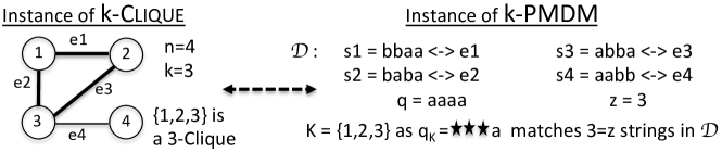
Figure 1: An example of the reduction from $k$-Clique to $k$-PMDM. The solution for both is $\{1,2,3\}$ as shown. Note that, for $k=4$, the instance of $4$-PMDM would need $z=6$ matches; neither this many matches can be found in $\mathcal{D}$ nor a $4$-clique can be found in the graph.

An example of the reduction from $k$-Clique to $k$-PMDM is shown in Figure 1. Our reduction shows that solving $k$-PMDM efficiently even for strings over a binary alphabet would imply a breakthrough for the $k$-Clique problem (see Appendix B for more details).

Any algorithm solving PMDM-Size can be trivially applied to solve $k$-PMDM.

Theorem 3.3.

PMDM-Size is NP-hard for strings over a binary alphabet.

4 Approximation Algorithm for PMDM

Clearly, PMDM is at least as hard as PMDM-Size because it also outputs the positions of the wildcards (set $K$). Thus, PMDM is also NP-hard. We show existence of a polynomial-time approximation algorithm for PMDM whose approximation factor is given with respect to $d$. The authors of [22] show a polynomial-time $\mathcal{O}(d^{1/4+\epsilon})$-approximation algorithm, for any constant $\epsilon>0$, for the Minimum Union (MU) problem. In Appendix C, we show a polynomial-time reduction from PMDM to MU that implies the following result.

Theorem 4.1.

For any constant $\epsilon>0$, there is a polynomial-time $\mathcal{O}(d^{1/4+\epsilon})$-approximation algorithm for PMDM.

In addition, the authors of [22] show that their $\mathcal{O}(d^{1/4+\epsilon})$-approximation algorithm for MU is tight under plausible complexity conjectures. In Appendix C, we also show that approximating the MU problem can be reduced to approximating PMDM in polynomial time and hence the same tightness results apply to PMDM.

Applying Theorem 4.1 to solve PMDM is not practical, as in real-world applications, such as those in Introduction, $d$ is typically in the order of thousands or millions [24, 28, 30, 57].

5 A Data Structure for PMDM Queries

We next show algorithms and data structures for the PMDM problem under the assumption that $2^{\ell}$ is reasonably small. Specifically, we consider the word-RAM model with $w$-bit machine words, where $w\!=\!\Omega(\log\!N+\ell)$. We measure space in terms of $w$-bit machine words and focus on showing space vs. query-time trade-offs for answering $q,z$ PMDM queries over $\mathcal{D}$. A summary of the complexities of the data structures is shown in Table 1. Specifically, algorithm Small-$\ell$ and data structure Simple are used as building blocks in the more involved data structure Split, shown in the following theorem.

Theorem 5.1.

There exists a data structure that answers $q,z$ PMDM queries over $\mathcal{D}$ in time $\mathcal{O}(2^{\ell/2}(2^{\ell/2}+\tau)\ell)$ and requires space $\mathcal{O}(2^{\ell}d^{2}/\tau^{2}+2^{\ell/2}d)$, for any parameter $\tau\in[1,d]$.

Algorithm Small-$\ell$: $\mathcal{O}(d\ell)$ Space, $\mathcal{O}(2^{\ell}\ell+d\ell)$ Query Time.

No data structure on top of the dictionary $\mathcal{D}$ is stored. In the query algorithm, we initialize an array $A$ of size $2^{\ell}$ with zeros. For every possible $\ell$-bit vector $i$, representing $K_{i}\subseteq\{1,\ldots,\ell\}$, $A[i]$ will finally store the number of strings in $\mathcal{D}$ that match $q_{K_{i}}=q\otimes K_{i}$. For every string $s\in\mathcal{D}$, we compute the set of positions in which $s$ and $q$ differ, and for this $K_{i}$, we increment $A[i]$. This computation takes $\mathcal{O}(d\ell)$ time and $\mathcal{O}(1)$ extra space. Then we apply a folklore dynamic-programming-based approach (cf. [2]) to count the number of strings matching $q_{K_{i}}$. This takes $\mathcal{O}(\ell 2^{\ell})$ time and $\mathcal{O}(2^{\ell})$ extra space. Thus, overall, the (query) time required by algorithm Small-$\ell$ is $\mathcal{O}(\ell 2^{\ell}\!+\!d\ell)$ and the space is $\mathcal{O}(2^{\ell}\!+\!d\ell)$.

Let us denote by $z_{0}\!\in\![1,d]$ the smallest $z$ value for which we support PMDM queries. We first present Simple, an auxiliary data structure, which we will apply later on to construct Split, a data structure with the space/query-time trade-off given by Theorem 5.1.

DS Simple: $\mathcal{O}(\genfrac{(}{)}{0.0pt}{1}{\ell}{k}\cdot d/z_{0})$ Space, $\mathcal{O}(\genfrac{(}{)}{0.0pt}{1}{\ell}{k})$ Query Time, for Fixed $k$.

For each possible subset of $\{1,\ldots,\ell\}$ of size $k$, we mask the $k$ corresponding positions in all strings from $\mathcal{D}$. We sort the masked strings lexicographically in order to have counts for each distinct (masked) string and construct a dictionary (hash map): the key is the fingerprint of a masked string (item) and the value is its count. The space occupied by the dictionary is $\mathcal{O}(\genfrac{(}{)}{0.0pt}{1}{\ell}{k}\cdot d/z_{0})$ by storing only the items (fingerprints of masked strings) whose count is at least $z_{0}$. Upon an on-line query $q$ of length $\ell$ with $z\geq z_{0}$, we attempt all possible masks of size $k$ for $q$ and read the count from the dictionary. All possible $\genfrac{(}{)}{0.0pt}{1}{\ell}{k}$ fingerprints can be computed in time $\mathcal{O}(\genfrac{(}{)}{0.0pt}{1}{\ell}{k})$ if we use a folklore algorithm for generating the combinations (cf. [9]) and a rolling hash function for the fingerprints, such as the classic Karp-Rabin (KR) fingerprints [40].

Note that $\genfrac{(}{)}{0.0pt}{1}{\ell}{k}$ can be asymptotically as large as $2^{\ell}/\sqrt{\ell}$, e.g. for $\ell=2k$. When $2^{\ell}=o(d)$, we manage to decrease the exponential dependency on $\ell$ in the space complexity, incurring extra time in the query. To this end, we next present the Split data structure.

Data structure	Space	Query time
Algorithm Small-$\ell$	$\mathcal{O}(d\ell)$	$\mathcal{O}(2^{\ell}\ell+d\ell)$
DS Simple	$\mathcal{O}(2^{\ell}d)$	$\mathcal{O}(2^{\ell})$
DS Split, any $\tau$	$\mathcal{O}(2^{\ell}d^{2}/\tau^{2}+2^{\ell/2}d)$	$\mathcal{O}(2^{\ell/2}\cdot(2^{\ell/2}+\tau)\ell)$
DS Split for $\tau=2^{\ell/4}\sqrt{d}$	$\mathcal{O}(2^{\ell/2}d)$	$\mathcal{O}(2^{\ell}\ell+2^{3\ell/4}\sqrt{d}\ell)$

Table 1: Basic complexities of the data structures from Section 5 (regardless of $k$ and $z_{0}$).

DS Split: $\mathcal{O}(2^{\ell}d^{2}/\tau^{2}+2^{\ell/2}d/z_{0})$ Space, $\mathcal{O}(2^{\ell/2}\cdot(2^{\ell/2}+\tau)\ell)$ Query Time, for any $\tau$.

This trade-off only makes sense for $\tau=\omega(\sqrt{d})$; otherwise the Simple data structure is better.

We split each string $p\in\mathcal{D}$ roughly in the middle, to prefix $p_{L}$ and suffix $p_{R}$; specifically, $p=p_{L}p_{R}$ and $|p_{L}|=\lceil\ell/2\rceil$. We create dictionaries $\mathcal{D}_{L}\!=\!\{p_{L}\!:\!p\!\in\!\mathcal{D}\}$ and $\mathcal{D}_{R}\!=\!\{p_{R}\!:\!p\!\in\!\mathcal{D}\}$. Let us now explain how to process $\mathcal{D}_{L}$; we process $\mathcal{D}_{R}$ analogously. Let $\lambda\!=\!\lceil\ell/2\rceil$. For each subset of $\{1,\ldots,\lambda\}$, we construct DS Simple over $\mathcal{D}_{L}$. This requires space $\mathcal{O}(2^{\ell/2}d/z_{0})$. Let $\tau$ be an input parameter, intuitively used as the minimum frequency threshold. For each of the possible $2^{\lambda}$ masks, we can have at most $\lfloor d/\tau\rfloor$ (masked) strings with frequency at least $\tau$. Over all masks, we thus have at most $2^{\lambda}\cdot\lfloor d/\tau\rfloor$ such strings; we call them $\tau$-frequent. For every pair of $\tau$-frequent strings, one from $\mathcal{D}_{L}$ and one from $\mathcal{D}_{R}$, we store the number of occurrences of their concatenation in $\mathcal{D}$. This requires space $\mathcal{O}(2^{\ell}d^{2}/\tau^{2})$.

Consider $\mathcal{D}_{L}$. For each mask $i$ and each string $p_{L}\in\mathcal{D}_{L}$, we can afford to store the list of all strings in $\mathcal{D}_{L}$ that match $p_{L}\otimes i$. Note that we have computed this information when sorting for constructing the Simple data structure over $\mathcal{D}_{L}$. This information requires space $\mathcal{O}(2^{\ell/2}d/z_{0})$. Thus, Split requires $\mathcal{O}(2^{\ell}d^{2}/\tau^{2}+2^{\ell/2}d/z_{0})$ space overall.

Let us now show how to answer an on-line $q,z$ query. We iterate over all possible $2^{\ell}$ masks performing exact computations and thus we can answer the query $q$ for any given $z$. Given mask $i$ we split $q^{\prime}=q\otimes i$ into two halves, $q^{\prime}_{L}$ and $q^{\prime}_{R}$ with $q^{\prime}=q^{\prime}_{L}q^{\prime}_{R}$ and $|q^{\prime}_{L}|=\lceil\ell/2\rceil$.

The intuition is that, if both halves are $\tau$-frequent, we have precomputed the frequency of their concatenation as explained above. If (at least) one of the two halves is $\tau$-infrequent we have to resort to the Small-$\ell$ algorithm to count exactly the frequency of $q$ using the list information enhancing the Simple data structure.

We distinguish among two cases: (i) one of the two halves is $\tau$-infrequent; or (ii) both halves are $\tau$-frequent. We first check if $q^{\prime}_{L}$ is $\tau$-infrequent using the data structure Simple we have constructed for $\mathcal{D}_{L}$. If so, we apply algorithm Small-$\ell$ on the following input: (i) the second half $q^{\prime}_{R}$ and (ii) a dictionary consisting of at most $\tau$ strings from $\mathcal{D}_{R}$ that correspond to the right halves of strings in $\mathcal{D}_{L}$ that match $q^{\prime}_{L}$. (Recall that the list of matches for $q^{\prime}_{L}$ is stored by our DS.) We proceed symmetrically if $q^{\prime}_{L}$ is $\tau$-frequent and $q^{\prime}_{R}$ is $\tau$-infrequent. Finally, if both $q^{\prime}_{L}$ and $q^{\prime}_{R}$ are $\tau$-frequent we read the corresponding precomputed counter from the hash map. In any of the two cases, if the frequency of $q^{\prime}$ is at least $z$, we return a positive answer. We obtain Theorem 5.1 by setting $z_{0}=1$.

We show, for completeness, how the Split data structure can be constructed in $\mathcal{O}(d2^{\ell})$ time. The Simple data structures for $\mathcal{D}_{L}$ and $D_{R}$ can be constructed in $\mathcal{O}(2^{\ell/2}d)$ time. We then create a hashmap for pairs of $\tau$-frequent strings. For each of the $2^{\ell}$ possible masks, say $i$, and each string $p\in\mathcal{D}$, we split $p^{\prime}=p\otimes i$ in the middle to obtain $p^{\prime}_{L}$ and $p^{\prime}_{R}$. If both $p^{\prime}_{L}$ and $p^{\prime}_{R}$ are $\tau$-frequent we increment a counter associated with $(p^{\prime}_{L},p^{\prime}_{R})$. Again, by using a folklore algorithm for generating the $2^{\ell}$ combinations and a rolling hash function for representing strings as KR fingerprints, we obtain a total construction time of $\mathcal{O}(d2^{\ell})$.

Comparison of the Data Structures.

Data structure Simple has lower query time than algorithm Small-$\ell$. However, its space complexity can be much higher. Data structure Split can be viewed as an intermediate option. For $\tau$ as in Table 1, it has better query time than algorithm Small-$\ell$ for $d=\omega(2^{3\ell/2})$, while keeping moderate space complexity. It always has worse query time than data structure Small, but its space complexity is lower by a factor of $2^{\ell/2}$. For example, for $d=2^{2\ell}$ we get the complexities shown in Table 2.

Data structure	Space	Query time
Algorithm Small-$\ell$	$\mathcal{O}(2^{2\ell}\ell)$	$\mathcal{O}(2^{2\ell}\ell)$
DS Simple	$\mathcal{O}(2^{3\ell})$	$\mathcal{O}(2^{\ell})$
DS Split for $\tau=2^{5\ell/4}$	$\mathcal{O}(2^{5\ell/2})$	$\mathcal{O}(2^{7\ell/4}\ell)$

Table 2: Basic complexities of the data structures from Section 5 for $d=2^{2\ell}$.

6 Exact Algorithms for a Bounded Number $k$ of Wildcards

We consider the following problem, which we solve by exact algorithms. These algorithms will form the backbone of our effective and efficient heuristic for the PMDM problem.

Heaviest $k$-PMDM
Input: A dictionary $\mathcal{D}$ of $d$ strings, each of length $\ell$, a string $q$ of length $\ell$, and a positive integer $k\leq d$. Output: A set $K\subseteq\{1,\ldots,\ell\}$ of size $k$ such that $q_{K}\!=\!q\!\otimes\!K$ matches the maximum number of strings in $\mathcal{D}$.

We will show the following result, which we will employ to solve the PMDM problem.

Theorem 6.1.

Heaviest $k$-PMDM for $k\!=\!\mathcal{O}(1)$ can be solved in $\mathcal{O}(N\!+\!\min\{N^{k/3},\ell^{k}\})$ time.

A hypergraph $H$ is a pair $(V,E)$, where $V$ is the set of nodes of $H$ and $E$ is a set of non-empty subsets of $V$, called hyperedges – in order to simplify terminology we will simply call them edges. Hypergraphs are a generalization of graphs in the sense that an edge can connect multiple nodes. Recall that the size of an edge is the number of nodes it contains. The rank of $H$, denoted by $r(H)$, is the maximum size of an edge of $H$.

We refer to a hypergraph $H\times K=(K,\{e:e\in E,e\subseteq K\})$, where $K$ is a subset of $V$, as a $|K|$-section. $H\times K$ is the hypergraph induced by $H$ on the nodes of $K$, and it contains all edges of $H$ whose elements are all in $K$. A hypergraph is weighted when each of its edges is associated with a weight. We define the weight of a weighted hypergraph as the sum of the weights of all of its edges. In what follows, we also refer to weights of nodes for conceptual clarity; this is equivalent to having a singleton edge of equal weight consisting of that node.

We define the following auxiliary problem on hypergraphs (see also [21]).

Heaviest $k$-Section
Input: A weighted hypergraph $H=(V,E)$ and a positive integer $k$. Output: A subset $K$ of size $k$ of $V$ such that $H\times K$ has maximum weight.

A polynomial-time $\mathcal{O}(n^{0.697831+\epsilon})$-approximation for Heaviest $k$-Section, for any $\epsilon>0$, for the case when all hyperedges of $H$ have size at most 3 was shown in [21] (see also [7]).

Two remarks are in place. First, we can focus on edges of size up to $k$ as larger edges cannot, by definition, exist in any $k$-section. Second, Heaviest $k$-Section is a generalization of the problem of deciding whether a $(c,k)$-hyperclique (i.e., a set of $k$ nodes whose subsets of size $c$ are all in $E$) exists in a graph, which in turn is a generalization of $k$-Clique. Unlike $k$-Clique, the $(c,k)$-hyperclique problem is not known to benefit from fast matrix multiplication in general; see [48] for a discussion on its hardness.

Lemma 6.2.

Heaviest $k$-PMDM can be reduced to Heaviest $k$-Section for a hypergraph with $\ell$ nodes and $d$ edges in $\mathcal{O}(N)$ time.

Proof 6.3.

We first compute the set $M_{s}$ of positions of mismatches of $q$ with each string $s\in\mathcal{D}$. We ignore strings from $\mathcal{D}$ that match $q$ exactly, as they will match $q$ after changing any set of letters of $q$ to wildcards. This requires $\mathcal{O}(d\ell)=\mathcal{O}(N)$ time in total.

Let us consider an empty hypergraph (i.e. with no edges) $H$ on $\ell$ nodes, numbered $1$ through $\ell$. Then, for each string $s\in\mathcal{D}$, we add $M_{s}$ to the edge-set of $H$ if $|M_{s}|\leq k$; if this edge already exists, we simply increment its weight by $1$.

We set the parameter $k$ of Heaviest $k$-Section to the parameter $k$ of Heaviest $k$-PMDM. We now observe that for $K\subseteq V$ with $|K|=k$, the weight of $H\times K$ is equal to the number of strings that would match $q$ after replacing with wildcards the $k$ letters of $q$ at the positions corresponding to elements of $K$. The statement follows.

An example of the reduction from Heaviest $k$-Section to Heaviest $k$-PMDM is shown in Figure 2.

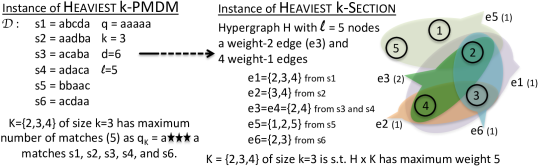
Figure 2: An example of the reduction from Heaviest $k$-Section to Heaviest $k$-PMDM. The solutions are at the bottom. Each edge has its weight in brackets and the total weight is $d=6$.

The next lemma gives a straightforward solution to Heaviest $k$-Section. It is analogous to algorithm Small-$\ell$ from Section 5, but without the optimization in computing sums of weights over subsets. It implies a linear-time algorithm for Heaviest $1$-Section.

Lemma 6.4.

Heaviest $k$-Section can be solved in $\mathcal{O}((2|V|)^{k}+|E|)$ time and $\mathcal{O}(|V|+|E|)$ space.

Proof 6.5.

Let us store a perfect hash map that maps every edge of $E$ to its weight (or 0 if the edge does not exist) [29]. This takes $\mathcal{O}(|E|)$ time. For every subset $K\subseteq V$ of size at most $k$, we sum the weights of all edges corresponding to its subsets. There are $\genfrac{(}{)}{0.0pt}{1}{|V|}{k}=\mathcal{O}(|V|^{k})$ choices for $|K|$, each having $2^{k}-1$ non-empty subsets. The stated time complexity follows.

We next show that for the cases $k=2$ and $k=3$, there exist more efficient solutions. In particular, we provide a linear-time algorithm for Heaviest $2$-Section.

Lemma 6.6.

Heaviest $2$-Section can be solved in $\mathcal{O}(|V|+|E|)$ time.

Proof 6.7.

Let $K$ be a set of nodes of size $2$ such that $H\times K$ has maximum weight. We decompose the problem in two cases. For each of the cases, we give an algorithm that considers several $2$-sections such that the heaviest of them has weight equal to that of $H\times K$.

Case 1. There is an edge $e=K$. For each edge $e\in E$ of size $2$, i.e. edge in the classical sense, we compute the sum of its weight and the weights of the nodes that it is incident to. This step requires $\mathcal{O}(|E|)$ time.

Case 2. There is no edge equal to $K$ in $E$. We compute $H\times\{v_{1},v_{2}\}$, where $v_{1},v_{2}$ are the two nodes with maximum weight, i.e. max and second-max. This step takes $\mathcal{O}(|V|)$ time.

In the end, we return the heaviest $2$-section among those returned by the algorithms for the two cases, breaking ties arbitrarily.

We next show that for $k=3$ the result of Lemma 6.4 can be improved when $|E|=o(|V|^{2})$.

Lemma 6.8.

Heaviest $3$-Section can be solved in $\mathcal{O}(|V|\cdot|E|)$ time and $\mathcal{O}(|V|+|E|)$ space.

Proof 6.9.

Let $K$ be a set of nodes of size $3$ such that $H\times K$ has maximum weight. We decompose the problem in the following three cases.

Case 1. There is an edge $e=K$. We go through each edge $e\in E$ of size $3$ and compute the weight of $H\times e$ in $\mathcal{O}(1)$ time. (We store the edges of $H$ in a perfect hash map [29].) This takes $\mathcal{O}(|E|)$ time in total. Let the edge yielding the maximum weight be $e_{\max}$.

Case 2. There is no edge of size larger than one in $H\times K$. We compute $H\times\{v_{1},v_{2},v_{3}\}$, where $v_{1},v_{2},v_{3}$ are the three nodes with maximum weight, i.e. max, second-max and third-max. This step takes $\mathcal{O}(|V|)$ time.

Case 3. There is an edge of size $2$ in $H\times K$. We can pick an edge $e$ of size $2$ from $E$ in $\mathcal{O}(|E|)$ ways and a node $v$ from $V$ in $\mathcal{O}(|V|)$ ways. We compute the weight of $H\times(e\cup\{v\})$ for all such pairs. Let the pair yielding maximum weight be $(e^{\prime},u^{\prime})$.

Finally, the maximum weight of $H\times K^{\prime}$ for $K^{\prime}\in\{\,e_{\max},\,\{v_{1},v_{2},v_{3}\},\,e^{\prime}\cup\{u^{\prime}\}\,\}$ is equal to the weight of $H\times K$, breaking ties arbitrarily.

Lemma 6.10.

Heaviest $k$-Section for an arbitrarily large constant $k\geq 4$ can be solved in $\mathcal{O}((|V|\cdot|E|)^{k/3})$ time and $\mathcal{O}(|V|+|E|)$ space.

Proof 6.11.

If $|E|>|V|^{2}$, then the simple algorithm of Lemma 6.4 solves the problem in time

$$\mathcal{O}((2|V|)^{k}+|E|)=\mathcal{O}(|V|^{k/3}(|V|^{2})^{k/3}+|E|)=\mathcal{O}((|V|\cdot|E|)^{k/3})$$

and linear space. We can thus henceforth assume that $|E|\leq|V|^{2}$.

Let $K$ be a set of nodes of size at most $k$ such that $H\times K$ has maximum weight. If $H\times K$ contains isolated nodes (i.e., nodes not contained in any edge), they can be safely deleted without altering the result. We can thus assume that $H\times K$ does not contain isolated nodes, and that $|V|\leq k|E|$ since otherwise the hypergraph $H$ would contain isolated nodes.

We first consider the case that $r(H\times K)>1$, i.e., there is an edge of $H\times K$ of size at least 2. We design a branching algorithm that constructs several candidate sets; the ones with maximum weight will have weight equal to that of $H\times K$. We start with set $X:=\emptyset$. For each set $X$ that we process, let $Z_{X}$ be the superset of $X$ of size at most $k$ such that $H\times Z_{X}$ has maximum weight. We have the following two cases:

Case 1. There is an edge $e$ in $H\times Z_{X}$ that contains at least two nodes from $Z_{X}\setminus X$. To account for this case, we select every possible such edge $e$, set $X:=X\cup e$, and continue the branching algorithm.

Case 2. Each edge in $H\times Z_{X}$ contains at most one node from $Z_{X}\setminus X$. In this case we conclude the branching algorithm as follows. We use a hash map of all the edges. For every node $v\in V\setminus X$ we compute its weight as the total weight of edges $Y\cup\{v\}\in E$ for $Y\subseteq X$, using the hash map in $\mathcal{O}(2^{k})=\mathcal{O}(1)$ time. Finally, in $\mathcal{O}(|V|k)=\mathcal{O}(|V|)$ time we select $k-|X|$ nodes with largest weights and insert them into $X$. The total time complexity of this step is $\mathcal{O}(|V|)$. This case also works if $|X|=k$ and then its time complexity is only $\mathcal{O}(1)$.

The correctness of this branching algorithm follows from an easy induction, showing that at every level of the branching tree there is a subset of $K$.

Let us now analyze the time complexity of this branching algorithm. Each branching in Case 1 takes $\mathcal{O}(|E|)$ time and increases the size of $|X|$ by at least 2. At every node of the branching tree we call the procedure of Case 2. It takes $\mathcal{O}(|V|)$ time if $|X|<k$.

If the procedure of Case 2 is called in a non-leaf node of the branching tree, then its $\mathcal{O}(|V|)$ running time is dominated by the $\mathcal{O}(|E|)$ time that is required for further branching since $|V|\leq k|E|$. Hence, it suffices to bound (a) the total time complexity of calls to the algorithm for Case 2 in leaves that correspond to sets $X$ such that $|X|<k$ and (b) the total number of leaves that correspond to sets $X$ such that $|X|=k$.

If $k$ is even, (a) is bounded by $\mathcal{O}(|E|^{(k-2)/2}|V|)$ and (b) is bounded by $\mathcal{O}(|E|^{k/2})$. Hence, (b) dominates (a) and we have

$$\mathcal{O}(|E|^{k/2})=\mathcal{O}(|E|^{k/3}|E|^{k/6})=\mathcal{O}(|E|^{k/3}|V|^{k/3}).$$ (1)

If $k$ is odd, (a) is bounded by $\mathcal{O}(|E|^{(k-1)/2}|V|)$ and (b) is bounded by $\mathcal{O}(|E|^{(k-1)/2})$, which is dominated by (a). By using (1) for $k-3$ we also have:

$$\mathcal{O}(|E|^{(k-1)/2}\cdot|V|)=\mathcal{O}(|E|^{(k-3)/2}\cdot|E|\cdot|V|)=\mathcal{O}((|E|\cdot|V|)^{(k-3)/3}\cdot|E|\cdot|V|)=\mathcal{O}((|E|\cdot|V|)^{k/3}).$$

We now consider the case that $r(H\times K)=1$. We use the algorithm for Case 2 above that works in $\mathcal{O}(|V|)$ time, which is $\mathcal{O}(|V|\cdot|E|)$.

Lemmas 6.2-6.10 imply Theorem 6.1, which we employ iteratively to obtain the following.

Theorem 6.12.

PMDM can be solved in time $\mathcal{O}(N+\min\{N^{k/3},\ell^{k}\})$ and space $\mathcal{O}(N)$ if $k=\mathcal{O}(1)$.

Proof 6.13.

We apply the reduction of Lemma 6.2 and obtain a hypergraph with $|V|=\ell$ and $|E|=d$. Starting with $k=1$ and for growing values of $k$, we solve Heaviest $k$-Section until we obtain a solution of weight at least $z$, employing either only Lemma 6.4, or Lemmas 6.4, 6.6, 6.8, 6.10 for $k=1,2,3$ and $k\geq 4$, respectively. PMDM can thus be solved in $\mathcal{O}(N+\min\{N^{k/3},\ell^{k}\})$ time and linear space.

7 Exact Algorithms for a Bounded Number $m$ of Query Strings

Recall that masking a potential match $(q_{1},q_{2})$ in record linkage can be performed by solving PMDM twice and superimposing the wildcards (see Section 1). In this section, we consider the following generalized version of PMDM to perform the masking simultaneously. The advantage of this approach is that it minimizes the final number of wildcards in $q_{1}$ and $q_{2}$.

Multiple Pattern Masking for Dictionary Matching (MPMDM)
Input: A dictionary $\mathcal{D}$ of $d$ strings, each of length $\ell$, a collection $\mathcal{M}$ of $m$ strings, each of length $\ell$, and a positive integer $z$. Output: A smallest set $K\subseteq\{1,\ldots,\ell\}$ such that, for every $q$ from $\mathcal{M}$, $q_{K}\!=\!q\!\otimes\!K$ matches at least $z$ strings from $\mathcal{D}$.

Let $N=d\ell$. We show the following theorem.

Theorem 7.1.

MPMDM can be solved in time $\mathcal{O}(N+\min\{N^{k/3}z^{m-1},\ell^{k}\})$ if $k=\mathcal{O}(1)$ and $m=\mathcal{O}(1)$.

We use a generalization of Heaviest $k$-Section in which the weights are $m$-tuples that are added and compared component-wise and we aim to find a subset $K$ such that the weight of $H\times K$ is at least $(z,\ldots,z)$. An analogue of Lemma 6.4 holds without any alterations, which accounts for the $\mathcal{O}(N+\ell^{k})$-time algorithm. We adapt the proof of Lemma 6.10 as follows. The branching remains the same, but we have to tweak the final step, that is, what happens when we are in Case 2. For $m=1$ we could simply select a number of largest weights, but for $m>1$ multiple criteria need to be taken into consideration. All in all, the problem reduces to the following variation on the Multiple-Choice Knapsack problem [41].

$\kappa$ Heaviest Vectors ($\kappa$-HV)
Input: A collection $\mathcal{T}$ of $t$ vectors from $\mathbb{Z}_{\geq 0}^{m}$, a vector $x$ from $\{0,\ldots,z\}^{m}$, for a positive integer $z$, and an integer $\kappa\in\{0,\ldots,t\}$. Output: Compute $\kappa$ elements of $\mathcal{T}$ (if they exist) such that if $y$ is their component-wise sum, $y[i]\geq x[i]$ for all $i\in\{1,\ldots,m\}$.

The exact reduction from Case 2 is as follows: the set $\mathcal{T}$ contains weights of subsequent nodes $v\in V\setminus X$ (defined as the sums of weights of edges $Y\cup\{v\}\in E$ for $Y\subseteq X$), so $t\leq|V|$, $x$ is $(z,\ldots,z)$ minus the sum of weights of all edges $e\in E$ such that $e\subseteq X$, and $\kappa=k-|X|$.

The solution to $\kappa$-HV is a rather straightforward dynamic programming.

Lemma 7.2.

For $\kappa,m=\mathcal{O}(1)$, $\kappa$-HV can be solved in time $\mathcal{O}(t\cdot z^{m-1})$.

Proof 7.3.

We apply dynamic programming. Let $\mathcal{T}=v_{1},\ldots,v_{t}$. We compute an array $A$ of size $\mathcal{O}(t\kappa z^{m-1})$ such that, for $i\in\{0,\ldots,t\}$, $j\in\{0,\ldots,\kappa\}$ and $v\in\{0,\ldots,z\}^{m-1}$,

$$A[i,j,v]=\max\{a\,:\,\exists S\subseteq\{v_{1},\ldots,v_{i}\},\,|S|=j,\,\sum_{u\in S}u=(v,a)\},$$

where $(v,a)$ denotes the operation of appending element $a$ to vector $v$. From each state $A[i,j,v]$ we have two transitions, depending on whether $v_{i+1}$ is taken to the subset or not. Each transition is computed in $\mathcal{O}(m)=\mathcal{O}(1)$ time. This gives time $\mathcal{O}(t\cdot z^{m-1})$ in total.

The array is equipped with a standard technique to recover the set $S$ (parents of states). The final answer is computed by checking, for each vector $v\in\{0,\ldots,z\}^{m-1}$ such that $v[i]\geq x[i]$, for all $i=1,\ldots,m-1$, if $A[t,\kappa,v]\geq x[m]$.

Overall, we pay an additional $\mathcal{O}(z^{m-1})$ factor in the complexity of handling of Case 2, which yields the complexity of Theorem 7.1.

8 Summary of Greedy Heuristic for PMDM and Experiments

We design a greedy heuristic for PMDM which, for a given constant $\tau\geq 1$, applies Theorem 6.1 iteratively, for some $k\leq\tau$. In iteration $i=1$, we apply Theorem 6.1 for $k=1,\ldots,\tau$ and check whether there are at least $z$ strings from $\mathcal{D}$ that can be matched when at most $k$ wildcards are substituted in the query string $q$. If at least $z$ such strings exist, we return the minimum such $k$ and terminate. Clearly, by Theorem 6.12, the returned solution $K_{1}$ is an optimal solution to PMDM. Otherwise, we proceed into the next iteration $i=2$. In this iteration, we construct string $q_{K_{1}}=q\otimes K_{1}$ and apply Theorem 6.1, for $k=1,\ldots,\tau$, to $q_{K_{1}}$. This returns a solution $K_{2}$ telling us whether there are at least $z$ strings from $\mathcal{D}$ that can be matched with $q_{K_{2}}=q_{K_{1}}\otimes K_{2}$. If there exist such strings, we return $K_{1}\cup K_{2}$ and terminate. Otherwise, we proceed into iteration $i=3$, which is analogous to iteration $i=2$. The time complexity of the heuristic is $\mathcal{O}((N+N^{\tau/3})\ell)$ and the space complexity is $\mathcal{O}(N)$. A complete description of the heuristic can be found in Appendix D.

An extensive experimental evaluation demonstrating the effectiveness and efficiency of the proposed heuristic on real datasets used in record linkage, as well as on synthetic datasets, is presented in Appendix E. In the experiments that we have performed, the proposed heuristic: (I) produced nearly-optimal solutions for varying values of $z$ and $\ell$, even when applied with a small $\tau$; and (II) scaled as predicted by the complexity analysis, requiring fewer than $3$ seconds for $d=6\cdot 10^{6}$ in all tested cases. These results suggest that our methods can inspire solutions in large-scale real-world systems, where no algorithms for PMDM exist.

Appendix A Other Related Work

• Dictionary Matching with $k$-errors: A similar line of research to that of Partial Match has been conducted under the Hamming and edit distances, where, in this case, $k$ is the maximum allowed distance between the query string and a dictionary string [62, 17, 26, 13, 18, 14]. The structure of Dictionary Matching with $k$-errors is very similar to Partial Match as each wildcard in the query string gives $|\Sigma|$ possibilities for the corresponding symbol in the dictionary strings. On the other hand, in Partial Match the wildcard positions are fixed. Cohen-Addad, Feuilloley and Starikovskaya showed that in the pointer machine model one cannot avoid exponential dependency on $k$ either in the space or in the query time [25].

• Enumerating Motifs with $k$-wildcards: Given an input string $s$ of length $n$ over an alphabet $\Sigma$ and positive integers $k$ and $z$, this problem asks to enumerate all motifs over $\Sigma\sqcup\{\star\}$ with up to $k$ wildcards that occur at least $z$ times in $s$. As the size of the output is exponential in $k$, the enumeration problem has such a lower bound. Several approaches exist for efficient motif enumeration, all aimed at reducing the impact of the output’s size: efficient indexing to minimise the output delay [31, 8]; exploiting a hierarchy of wildcards positions according to the number of occurrences [12]; or defining a subset of motifs of fixed-parameter tractable size (in $k$ or $z$) that can generate all the others [51, 6, 54].

Appendix B On the Hardness of $k$-Clique

Our reduction (Theorem 3.1) shows that solving $k$-PMDM efficiently even for strings over a binary alphabet would imply a breakthrough for the $k$-Clique problem for which it is known that, in general, no fixed-parameter tractable algorithm with respect to parameter $k$ exists unless the Exponential Time Hypothesis (ETH) fails [36]. That is, $k$-Clique has no $f(k)n^{o(k)}$ time algorithm, and is thus W[1]-complete (again, under the ETH hypothesis). On the upper bound side, $k$-Clique can be trivially solved in $\mathcal{O}(n^{k})$ time (enumerating all subsets of nodes of size $k$), and this can be improved to $\mathcal{O}(n^{\omega k/3})$ time for $k$ divisible by $3$ using square matrices multiplication ($\omega$ is the exponent of square matrix multiplication). However, for general $k\geq 3$ and any constant $\epsilon>0$, the $k$-Clique hypothesis states that there is no $\mathcal{O}(n^{(\omega/3-\epsilon)k})$-time algorithm and no combinatorial $\mathcal{O}(n^{(1-\epsilon)k})$-time algorithm [20, 48, 61].

Given an undirected graph $G$, an independent set is a subset of nodes of $G$ such that no two distinct nodes of the subset are adjacent. Let us note that the problem of computing a maximum clique in a graph $G$, which is equivalent to that of computing the maximum independent set in the complement of $G$, cannot be $n^{1-\epsilon}$-approximated in polynomial time, for any $\epsilon>0$, unless $\text{P}=\text{NP}$ [32, 63].

Appendix C Material Omitted from the Approximation Algorithm for PMDM

Let us start by defining the Minimum Union (MU) problem [22].

Minimum Union (MU)
Input: A collection $\mathcal{S}$ of $d$ sets over a universe $U$ and a positive integer $z\leq d$. Output: A collection $\mathcal{T}\subseteq\mathcal{S}$ with $|\mathcal{T}|=z$ such that the size of $\cup_{S\in\mathcal{T}}S$ is minimized.

To illustrate the MU problem, consider an instance of it where $U=\{1,2,3,4,5\}$, $\mathcal{S}=\{\{1\},\{1,2,3\},\{1,3,5\},\{3\},\{3,4,5\},\{4\},\{4,5\},\{5\}\}$, with $d=|\mathcal{S}|=8$, and $z=4$. Then $\mathcal{T}=\{\{3\},\{3,4,5\},\{4\},\{4,5\}\}$ is a solution because $|\mathcal{T}|=z=4$ and $|\cup_{S\in\mathcal{T}}S|=3$ is minimum. The MU problem is NP-hard and the following approximation result is known.

Theorem C.1 ([22]).

For any constant $\epsilon>0$, there is a polynomial-time $\mathcal{O}(d^{1/4+\epsilon})$-approximation algorithm for MU.

Theorem C.2.

PMDM can be reduced to MU in polynomial time.

Proof C.3.

We reduce the PMDM problem to MU in polynomial time as follows. Given any instance $\mathcal{I}_{\textsc{PMDM}}$ of PMDM, we construct an instance $\mathcal{I}_{\text{MU}}$ of MU in time $\mathcal{O}(d\ell)$ by performing the following steps:

1. The universe $U$ is set to $\{1,\ldots,\ell\}$.

2. We start with an empty collection $\mathcal{S}$. Then, for each string $s_{i}$ in $\mathcal{D}$, we add member $S_{i}$ to $\mathcal{S}$, where $S_{i}$ is the set of positions where string $q$ and string $s_{i}$ have a mismatch. This can be done trivially in time $\mathcal{O}(d\ell)$ for all strings in $\mathcal{D}$.

3. Set the $z$ of the MU problem to the $z$ of the PMDM problem.

Thus, the total time $\mathcal{O}(d\ell)$ needed for Steps 1 to 3 above is clearly polynomial in the size of $\mathcal{I}_{\textsc{PMDM}}$. To conclude the proof, it remains to show that given a solution $\mathcal{T}$ to $\mathcal{I}_{\text{MU}}$ we can obtain a solution $K$ to $\mathcal{I}_{\textsc{PMDM}}$ in time polynomial in the size of $\mathcal{I}_{\text{MU}}$, and that for each solution $K$ to $\mathcal{I}_{\textsc{PMDM}}$, there exists a corresponding solution $\mathcal{T}$ to $\mathcal{I}_{\text{MU}}$.

($\Rightarrow$) If $\mathcal{T}\subseteq\mathcal{S}$ is a solution to $\mathcal{I}_{\text{MU}}$, then we can construct a string $q_{K}\!=\!q\!\otimes\!K$ that corresponds to $\mathcal{T}$ and is a solution to $\mathcal{I}_{\textsc{PMDM}}$. The construction of $q_{K}$ can be performed in polynomial time by setting $q_{K}=q$ and then substituting the positions of $q_{K}$ corresponding to the elements of the sets of $\mathcal{T}$ with wildcards. $K$ is a solution to $\mathcal{I}_{\textsc{PMDM}}$ because: (I) Since $|\mathcal{T}|=z$, string $q_{K}$ matches at least $z$ strings in $\mathcal{D}$. (II) Since $|\cup_{S\in\mathcal{T}}S|$ is minimized, string $q_{K}$ has the minimum number of wildcards.

($\Leftarrow$) The output of PMDM is a set $K$ for matching at least $z$ strings but the output of MU is a collection $\mathcal{T}$ of size exactly $z$, and so some work is required. If $K$ is a solution to $\mathcal{I}_{\textsc{PMDM}}$, we can obtain a solution $\mathcal{T}\subseteq\mathcal{S}$ to $\mathcal{I}_{\text{MU}}$ using a greedy approach. Let $\mathcal{D}^{\prime}\subseteq\mathcal{D}$ be the collection of strings in $\mathcal{D}$ that match $q_{K}\!=\!q\!\otimes\!K$ and $\mathcal{S}^{\prime}\subseteq\mathcal{S}$ be the collection of sets of mismatches corresponding to the strings in $\mathcal{D}^{\prime}$. To construct $\mathcal{T}$, we select any $z$ sets $S^{\prime}_{1}$, $\ldots$, $S^{\prime}_{z}$ from $\mathcal{S}^{\prime}$. Collection $\mathcal{S}^{\prime}$ contains at least $z$ sets due to Step 1 above and the fact that $K$ is a solution to $\mathcal{I}_{\textsc{PMDM}}$. The correctness of this approach is implied by the fact that, if there is a $\mathcal{T}$ such that $|\mathcal{T}|=z$ and $\cup_{S\in\mathcal{T}}S=K$, then we would find it. Further, it is not possible that these $z$ sets do not cover $K$. In that case, there would be $z$ sets in $\mathcal{S}$ whose union is a proper subset $K^{\prime}$ of $K$, which is a contradiction as $q_{K}^{\prime}$ would have fewer wildcards than $q_{K}$ and $K^{\prime}$ would be a solution to $\mathcal{I}_{\textsc{PMDM}}$. $\mathcal{T}$ is a solution to $\mathcal{I}_{\text{MU}}$ because: (I) $|\mathcal{T}|=z$ by construction, and (II) $|\cup_{S\in\mathcal{T}}S|$ is minimized because, by definition, the size of $K$ is minimized, which implies that $|\cup_{S\in\mathcal{S}^{\prime}}S|=|\cup_{S\in\mathcal{T}}S|$ is also minimized.

Proof of Theorem 4.1.

The reduction in Theorem C.2 implies that there is a polynomial-time approximation algorithm for PMDM. In particular, Theorem C.1 provides an approximation guarantee for MU that depends on the number of sets of the input $\mathcal{S}$. In Step 2 of the reduction of Theorem C.2, we construct one set for the MU instance per one string of the dictionary $\mathcal{D}$ of the PMDM instance. Also, from the constructed solution $\mathcal{T}$ to the MU instance, we obtain a solution $K$ to the PMDM instance by simply substituting the positions of $q$ corresponding to the elements of the sets of $\mathcal{T}$ with wildcards. This construction implies the approximation result of Theorem 4.1 that depends on the size of $\mathcal{D}$. We obtain Theorem 4.1.∎

Sanity Check.

Theorem 3.1 (reduction from $k$-Clique to $k$-PMDM) and Theorem 4.1 (approximation algorithm for PMDM) do not contradict the inapproximability results for the maximum clique problem (see Appendix B), since our reduction from $k$-Clique to $k$-PMDM cannot be adapted to a reduction from maximum clique to PMDM-Size.

Two-Way Reduction.

The reader can probably share the intuition that the opposite to the reduction of Theorem C.2 is easy to prove. We give this proof next for completeness.

Theorem C.4.

MU can be reduced to PMDM in polynomial time.

Proof C.5.

We reduce the MU problem to the PMDM problem in polynomial time as follows. Let $\ell=||\mathcal{S}||$ denote the total number of elements in the $d$ members of $\mathcal{S}$. Given any instance $\mathcal{I}_{\text{{MU}}}$ of MU, we construct an instance $\mathcal{I}_{\textsc{PMDM}}$ of PMDM by performing the following steps:

1. Set the query string $q$ equal to the string $\texttt{a}^{\ell}$ of length $\ell$. This can be done in $\mathcal{O}(\ell)$ time.

2. After sorting the union of all elements of members of $\mathcal{S}$, we can assign to each element $j$ a unique rank $\textsf{rank}(j)\in\{1,\ldots,\ell\}$. For each set $S_{i}$ in $\mathcal{S}$, construct a string $s_{i}=\texttt{a}^{\ell}$, set $s_{i}[\textsf{rank}(j)]:=\texttt{b}$ if and only if $j\in S_{i}$, and add $s_{i}$ to dictionary $\mathcal{D}$. This can be done in $\mathcal{O}(d\ell+\ell\log\ell)$ time.

3. Set the $z$ of the PMDM problem equal to the $z$ of the MU problem. This can be done in $\mathcal{O}(1)$ time.

Thus, the total time $\mathcal{O}(d\ell+\ell\log\ell)$ needed for Steps 1 to 3 above is clearly polynomial in the size of $\mathcal{I}_{\textsc{MU}}$. To conclude the proof, it remains to show that, given a solution $K$ to $\mathcal{I}_{\textsc{PMDM}}$, we can obtain a solution $\mathcal{T}$ to $\mathcal{I}_{\text{MU}}$ in time polynomial in the size of $\mathcal{I}_{\textsc{PMDM}}$, and that for each solution $\mathcal{T}$ to $\mathcal{I}_{\text{MU}}$ there exists a corresponding solution $K$ in $\mathcal{I}_{\textsc{PMDM}}$.

($\Rightarrow$) Let us first show how to obtain a solution $\mathcal{T}$ to $\mathcal{I}_{\text{{MU}}}$ from a solution string $q_{K}\!=\!q\!\otimes\!K$ to $\mathcal{I}_{\text{{PMDM}}}$ in polynomial time in the size of $\mathcal{I}_{\textsc{PMDM}}$. $K$ corresponds to the minimized $\cup_{S\in\mathcal{T}}S$ of $\mathcal{I}_{\textsc{MU}}$. We now need to construct a solution $\mathcal{T}$ by picking up exactly $z$ sets $S^{\prime}_{1},S^{\prime}_{2},\ldots,S^{\prime}_{z}$ of $\mathcal{S}$ such that the rank of every element $j$ of $S^{\prime}_{i}$, $i\in[1,z]$, is also an element of $K$ and every element of $K$ is covered by at least one $\textsf{rank}(j)$ for some $i,j$ such that $j\in S^{\prime}_{i}$. This can be done using a greedy approach. We first select all sets $S^{\prime}_{1},S^{\prime}_{2},\ldots,S^{\prime}_{z^{\prime}}$ from $\mathcal{S}$ such that the rank of every element $j$ of $S^{\prime}_{i}$, $i\in[1,z^{\prime}]$, is also an element of $K$. Note that by construction we have at least $z$ such sets (i.e. $z^{\prime}\geq z$) because they correspond to at least $z$ strings in $\mathcal{D}$ that have b in a subset of the positions in $K$. This selection can be done in $\mathcal{O}(\ell)$ time using perfect hashing [29]. We now construct $\mathcal{T}$ by starting from the empty collection and adding to it any $z$ sets from $S^{\prime}_{1},S^{\prime}_{2},\ldots,S^{\prime}_{z^{\prime}}$. The correctness of this approach is implied by the fact that if there is a $\mathcal{T}$ such that $|\mathcal{T}|=z$ and $\cup_{S\in\mathcal{T}}S=K$ then we would find it. It is not possible that we would need more than these $z$ sets to cover $K$. In that case, there would be $z$ sets that could cover a proper subset $K^{\prime}$ of $K$ (i.e., there would be a $q_{K}^{\prime}\!=\!q\!\otimes\!K^{\prime}$ with fewer wildcards than $q_{K}\!=\!q\!\otimes\!K$ so that $K^{\prime}$ is also a solution to $\mathcal{I}_{\textsc{PMDM}}$) which is a contradiction. The whole process takes polynomial time in the size of $\mathcal{I}_{\textsc{PMDM}}$.

If $K$ is a solution to $\mathcal{I}_{\textsc{PMDM}}$ then $\mathcal{T}$ is a solution to $\mathcal{I}_{\text{MU}}$ because: (I) The set $K$ corresponds to at least $z$ strings in $\mathcal{D}$ by the definition of PMDM, which in turn by construction corresponds to $z$ sets of $\mathcal{S}$ (Step 3 of the reduction and greedy selection of $z$ sets). (II) The size of $K$ is minimized by the definition of PPSM, which implies that the number of distinct occurrences (positions) of b in the strings of $\mathcal{D}$ that are equal to the positions of $\star$’s in $q_{K}\!=\!q\!\otimes\!K$ is also minimized. Since each such position corresponds to a unique rank in $\mathcal{S}$ by construction (Step 3 of the reduction), it holds that $|\cup_{S\in\mathcal{S}}S|$ is minimized. From I and II, it holds that $\mathcal{T}$ is a solution to $\mathcal{I}_{\textsc{MU}}$.

($\Leftarrow$) If $\mathcal{T}$ is a solution to $\mathcal{I}_{\textsc{MU}}$, then $K$ is a solution to $\mathcal{I}_{\textsc{PMDM}}$ because: (I) Since $|\mathcal{T}|=z$, string $q_{K}\!=\!q\!\otimes\!K$ matches at least $z$ strings in $\mathcal{D}$. (II) Since $|\cup_{S\in\mathcal{T}}S|$ is minimized, $q_{K}$ has the minimum number of $\star$’s. From I and II, it holds that $K$ is a solution to $\mathcal{I}_{\textsc{PMDM}}$.

Appendix D A Greedy Heuristic for PMDM

For completeness, we provide a full description of the heuristic outlined in Section 8 below.

We design a heuristic called Greedy $\tau$-PMDM which, for a given constant $\tau\geq 1$, applies iteratively Theorem 6.1, for $k=1,\ldots,\tau$. Intuitively, the larger the $\tau$ the more effective but the slower Greedy $\tau$-PMDM is. Specifically, in iteration $i=1$, we apply Theorem 6.1 for $k=1,\ldots,\tau$ and check whether there are at least $z$ strings from $\mathcal{D}$ that can be matched when at most $k$ wildcards are substituted in the query string $q$. If there are, we return the minimum such $k$ and terminate. Clearly, by Theorem 6.12, the returned solution $K_{1}$ is an optimal solution to PMDM. Otherwise, we proceed into the next iteration $i=2$. In this iteration, we construct string $q_{K_{1}}=q\otimes K_{1}$ and apply Theorem 6.1, for $k=1,\ldots,\tau$, to $q_{K_{1}}$. This returns a solution $K_{2}$ telling us whether there are at least $z$ strings from $\mathcal{D}$ that can be matched with $q_{K_{2}}=q_{K_{1}}\otimes K_{2}$. If there are, we return $K_{1}\cup K_{2}$, which is now a (sub-optimal) solution to PMDM, and terminate. Otherwise, we proceed into iteration $i=3$, which is analogous to iteration $i=2$. Note that Greedy $\tau$-PMDM always terminates with some (sub-optimal) solution $K_{1}\cup K_{2}\cup\cdots\cup K_{j}$, for some $j\leq\lceil\ell/\tau\rceil$. Namely, in the worst case, it returns set $\{1,\ldots,\ell\}$ after $\lceil\ell/\tau\rceil$ iterations and $q_{\{1,\ldots,\ell\}}$ matches all strings in $\mathcal{D}$. The reason why Greedy $\tau$-PMDM does not guarantee finding an optimal solution to PMDM is that at iteration $i$ we fix the positions of wildcards based on solution $K_{1}\cup\cdots\cup K_{i-1}$. Since $\tau=\mathcal{O}(1)$, the time complexity of Greedy $\tau$-PMDM is $\mathcal{O}((N+N^{\tau/3})\ell)$: each iteration takes time $\mathcal{O}(N+N^{\tau/3})$ by Theorem 6.1, and then there are no more than $\lceil\ell/\tau\rceil=\mathcal{O}(\ell)$ iterations. The space complexity of Greedy $\tau$-PMDM is $\mathcal{O}(N)$. The hypergraph $H=(V,E)$ used in the implementation of Theorem 6.1 has edges of size up to $k$. If every string in $\mathcal{D}$ has more than $k$ mismatches with $q$, all edges in $H$ have size larger than $k$. In this case, we preprocess $H$, removing selected nodes and edges from it, so that it has at least one edge of size up to $k$ and then apply Greedy $\tau$-PMDM.

Hypergraph Preprocessing.

Let us now complete the algorithm by describing the hypergraph preprocessing. We want to ensure that hypergraph $H=(V,E)$ has at least one edge of size up to $k$ so that Greedy $\tau$-PMDM can be applied. To this end, if there is no edge of size up to $k$ at some iteration, we add some nodes into the partial solution with the following heuristic. We assign a score $s(u)$ to each node $u$ in $V$ using the function:

$$s(u)=|E_{u}|\cdot\frac{\sum_{e\in E_{u}}w(e)}{\sum_{e\in E_{u}}|e|},$$

where $E_{u}=\{e\in E:u\in e\}$ and $w(e)$ is the edge weight. Then, we add the node with maximum score from $H$ (breaking ties arbitrarily) into the partial solution and update the edges accordingly. This process is repeated until there is at least one edge of size up to $k$; it takes $\mathcal{O}(d\ell^{2})$ time. After that, we add the removed nodes into the current solution $K_{k}$ and use the resultant hypergraph when we apply Greedy $\tau$-PMDM.

The intuition behind the above process is to add nodes which appear in many short edges (so that we mask few positions) with large weight (so that the masked positions greatly increase the number of matched strings). We have also tried a different scoring function $s^{\prime}(u)=\sum_{e\in E_{u}}\frac{w(e)}{|e|}$ instead of $s(u)$, but the results were worse in terms of AvgRE and AvgSS, so we have omitted them.

Appendix E Experimental Evaluation

Methods.

We compared the performance of our heuristic Greedy $\tau$-PMDM (GR $\tau$), for the values $\tau\in[3,5]$, for which its time complexity is subquadratic in $N$, to the following two algorithms:

• Baseline (BA). In iteration $i$, BA adds a node of hypergraph $H$ into $K$ and updates $H$ according to the preprocessing described in Appendix D. If at least $z$ strings from $\mathcal{D}$ match the query string $q$ after the positions in $q$ corresponding to $K$ are replaced with wildcards, BA returns $K$ and terminates; otherwise, it proceeds into iteration $i+1$. Note that BA generally constructs a suboptimal solution $K$ to PMDM and takes $\mathcal{O}(d\ell^{2})$ time.

• Bruteforce (BF). In iteration $i$, BF applies Lemma 6.4 in the process of obtaining an optimal solution $K$ of size $i=k$ to PMDM. In particular, it checks whether at least $z$ strings from $\mathcal{D}$ match the query string $q$, after the $i$ positions in $q$ corresponding to $K$ are replaced with wildcards. If the check succeeds, BF returns $K$ and terminates; otherwise, it proceeds into iteration $i+1$. BF takes $\mathcal{O}(k(2\ell)^{k}+dk)$ time (see Lemma 6.4).

We used our own baseline in the evaluation, since there are no existing algorithms for addressing PMDM, as mentioned in Introduction. We have implemented all of the above algorithms in C++. Our implementations can be made available upon request.

Datasets.

We used the North Carolina Voter Registration database [3] (NCVR); a standard benchmark dataset for record linkage [24, 28, 38, 59]. NCVR is a collection of 7,736,911 records with attributes such as Forename, Surname, City, County, and Gender. We generated 4 subcollections of NCVR: (I) FS is comprised of all 952,864 records having Forename and Surname of total length $\ell=15$; (II) FCi is comprised of all 342,472 records having Forename and City of total length $\ell=15$; (III) FCiCo is comprised of all 342,472 records having Forename, City, and County of total length $\ell=30$; and (IV) FSCiCo is comprised of all 8,238 records having Forename, Surname, City and County of total length $\ell=45$.

We also generated a synthetic dataset, referred to as SYN, using the IBM Synthetic Data Generator [1], a standard tool for generating sequential datasets [27, 34]. SYN contains a collection of $6\cdot 10^{6}$ records, each of length $\ell=50$, over an alphabet of size $|\Sigma|=10$. We also used subcollections of SYN comprised of $x\cdot 10^{6}$ records of length $y$, each referred to as SYN_x.y.

Comparison Measures.

We evaluated the effectiveness of the algorithms using: (I) An Average Relative Error (AvgRE) measure, computed as avg${}_{i\in[1,1000]}\frac{k_{i}-k^{*}_{i}}{k^{*}_{i}}$, where $k_{i}^{*}$ is the size of the optimal solution, produced by BF, and $k_{i}$ is the size of the solution produced by one of the other tested algorithms. Both $k_{i}^{*}$ and $k_{i}$ are obtained by using, as query $q_{i}$, a record of the input dictionary selected uniformly at random. (II) An Average Solution Size (AvgSS) measure computed as avg${}_{i\in[1,1000]}k^{*}_{i}$ for BF and avg${}_{i\in[1,1000]}k_{i}$ for any other algorithm. We evaluated efficiency by reporting avg${}_{i\in[1,1000]}t_{i}$, where $t_{i}$ is the elapsed time of a tested algorithm to obtain a solution for query $q_{i}$ over the input dictionary.

Execution Environment.

We used a PC with Intel Xeon E5-2640@2.66GHz and 160GB RAM running GNU/Linux; and compiler gcc v.7.3.1 at optimization level -O3.

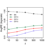
(a) $d\!=\!952,\!864$ and $\ell=15$

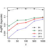
(b) $d\!=\!342,\!472$ and $\ell=15$

(c) $d\!=\!952,\!864$ and $\ell=15$

Figure 3: AvgRE vs. $z$ for (a) FS and (b) FCi; AvgSS for (c) FS.

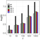
(a) $d\!=\!342,\!472$ and $\ell=15$

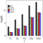
(b) $d\!=\!342,\!472$ and $\ell=30$

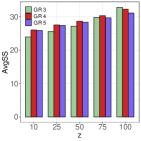
(c) $d\!=\!8,\!238$ and $\ell=45$

Figure 4: AvgSS vs. $z$ for (a) FCi. (b) FCiCo (BF did not produce results for any $z$ within 48 hours), and (c) FSCiCo (BF and BA did not produce results for any $z$ within 48 hours. The results for GR for $z\!>\!100$ are omitted; AvgSS$>\!40$).

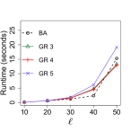
(a) $d\!=\!6\!\cdot\!10^{6}$ and $z\!=\!100$

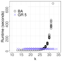
(b) $\ell\!=\!50$ and $z\!=\!100$

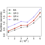
(c) $\ell\!=\!30$ and $z\!=\!100$

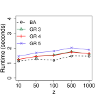
(d) $d\!=\!6\!\cdot\!10^{6}$ and $\ell\!=\!30$

Figure 5: Efficiency vs. (a) $\ell$ for SYN, (b) $k$ for SYN, (c) $d$ for SYN_x.30, $x\in\{1\cdot 10^{6},2\cdot 10^{6},\ldots,6\cdot 10^{6}\}$, and (d) $z$ for SYN. The results of BF are omitted, because it was slower than other methods by at least two orders of magnitude on average.

Effectiveness.

Figures 3 and 4(a) show that GR produced nearly-optimal solutions, significantly outperforming BA. In Figure 3(a), the solutions of GR 3 were no more than $9\%$ worse than the optimal, while those of BA were up to $95\%$ worse. In Figure 4(a), the average solution size of BF was $5.4$ vs. $5.9$ and $9$, for the solution size of GR 3 and BA, respectively.

In Figures 4(b) and 4(c), we examined the effectiveness of GR for larger $\ell$ values. Figure 4(b) shows that the solution size of GR 3 was at least $31\%$ and up to $60\%$ smaller than that of BA on average, while Figure 4(c) shows that the solution of GR 3 was comparable to that of GR 4 and 5. We omit the results for BF from Figures 4(b) and 4(c) and those for BA from Figure 4(c), as these algorithms did not produce results for all queries within 48 hours, for any $z$. This is because, unlike GR, BF does not scale well with $\ell$ and BA does not scale well with the solution size, as we will explain later.

Note that increasing $\tau$ generally increases the effectiveness of GR as it computes more positions of wildcards per iteration. However, even with $\tau=3$, it remains competitive to BF.

Efficiency.

Having shown that GR produced nearly-optimal solutions, we now show that it is comparable in terms of efficiency or faster than BA for synthetic data. (BF was at least two orders of magnitude slower than the other methods on average and thus we omit its results.) The results for NCVR were qualitatively similar (omitted). Figure 5(a) shows that GR spent, on average, the same time for a query as BA did. However, it took significantly (up to $36$ times) less time than BA for queries with large solution size $k$. This can be seen from Figure 5(b), which shows the time each query with solution size $k$ took; the results for GR 3 and 4 were similar and thus omitted. The reason is that BA updates the hypergraph every time a node is added into the solution, which is computationally expensive when $k$ is large. Figures 5(c) and 5(d) show that all algorithms scaled sublinearly with $d$ and with $z$, respectively. The increase with $d$ is explained by the time complexity of the methods. The slight increase with $z$ is because $k$ gets larger, on average, as $z$ increases. GR 3 and 4 performed similarly to each other, being faster than GR 5 in all experiments as expected: increasing $\tau$ from 3 or 4 to 5 trades-off effectiveness for efficiency.

Figures 6(a), 6(b), and 6(c) show the average solution size in the experiments of Figure 5(a), 5(c), and 5(d), respectively. Observe that the results are analogous to those obtained using the NCVR datasets: GR outperforms BA significantly. Also, observe in Figure 6(c) that the solution size of each tested algorithm gets larger, on average, as $z$ increases.

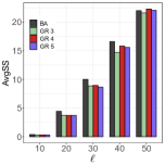
(a) $d=6\cdot 10^{6}$, $z=100$

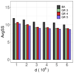
(b) $\ell=30$, $z=100$

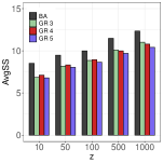
(c) $d=6\cdot 10^{6}$, $\ell=30$

Figure 6: AvgSS vs. (a) $\ell$ for SYN, (b) $d$ for SYN_x.30, $x\in\{1\cdot 10^{6},2\cdot 10^{6},\ldots,6\cdot 10^{6}\}$, and (c) $z$ for SYN.

References

- [1] IBM Synthetic Data Generator for Itemsets and Sequences. https://github.com/zakimjz/IBMGenerator, April 2020.
- [2] “Memory optimized, super easy to code” algorithm. https://codeforces.com/blog/entry/45223, June 2020.
- [3] North Carolina Voter Registration database (dataset ncvoter_Statewide.zip). https://dl.ncsbe.gov/?prefix=data/, April 2020.
- [4] Peyman Afshani and Jesper Sindahl Nielsen. Data structure lower bounds for document indexing problems. In 43rd International Colloquium on Automata, Languages and Programming (ICALP), volume 55 of LIPIcs, pages 93:1–93:15, 2016. doi:10.4230/LIPIcs.ICALP.2016.93.
- [5] Alfred V. Aho and Margaret J. Corasick. Efficient string matching: An aid to bibliographic search. Comm. of the ACM, 18(6):333–340, 1975. doi:10.1145/360825.360855.
- [6] Alberto Apostolico and Laxmi Parida. Incremental paradigms of motif discovery. J. Comput. Biology, 11(1):15–25, 2004. doi:10.1089/106652704773416867.
- [7] Benny Applebaum. Pseudorandom generators with long stretch and low locality from random local one-way functions. SIAM J. Computing, 42(5):2008–2037, 2013. doi:10.1137/120884857.
- [8] Hiroki Arimura and Takeaki Uno. An efficient polynomial space and polynomial delay algorithm for enumeration of maximal motifs in a sequence. J. Comb. Optim., 13(3):243–262, 2007. doi:10.1007/s10878-006-9029-1.
- [9] Lorraine A. K. Ayad, Carl Barton, Panagiotis Charalampopoulos, Costas S. Iliopoulos, and Solon P. Pissis. Longest common prefixes with k-errors and applications. In 25th International Symposium on String Processing and Information Retrieval (SPIRE), volume 11147 of Springer LNCS, pages 27–41, 2018. doi:10.1007/978-3-030-00479-8_3.
- [10] David R. Bailey, Alexis J. Battle, Benedict A. Gomes, and P. Pandurang Nayak. Estimating confidence for query revision models, U.S. Patent US7617205B2 (granted to Google), 2009.
- [11] Martha Bailey, Connor Cole, Morgan Henderson, and Catherine Massey. How well do automated linking methods perform? Lessons from U.S. historical data. NBER Working Papers 24019, National Bureau of Economic Research, Inc, 2017.
- [12] Giovanni Battaglia, Davide Cangelosi, Roberto Grossi, and Nadia Pisanti. Masking patterns in sequences: A new class of motif discovery with don’t cares. Theor. Computer Science, 410(43):4327–4340, 2009. doi:10.1016/j.tcs.2009.07.014.
- [13] Djamal Belazzougui. Faster and space-optimal edit distance "1" dictionary. In 20th Annual Symposium on Combinatorial Pattern Matching, (CPM), volume 5577 of Springer LNCS, pages 154–167, 2009. doi:10.1007/978-3-642-02441-2_14.
- [14] Djamal Belazzougui and Rossano Venturini. Compressed string dictionary search with edit distance one. Algorithmica, 74(3):1099–1122, 2016. doi:10.1007/s00453-015-9990-0.
- [15] Philip Bille, Inge Li Gørtz, Hjalte Wedel Vildhøj, and Søren Vind. String indexing for patterns with wildcards. Theory Computing System, 55(1):41–60, 2014. doi:10.1007/s00224-013-9498-4.
- [16] Allan Borodin, Rafail Ostrovsky, and Yuval Rabani. Lower bounds for high dimensional nearest neighbor search and related problems. In 31st ACM Symposium on Theory of Computing (STOC), pages 312–321, 1999. doi:10.1145/301250.301330.
- [17] Gerth Stølting Brodal and Srinivasan Venkatesh. Improved bounds for dictionary look-up with one error. Inf. Processing Letters, 75(1-2):57–59, 2000. doi:10.1016/S0020-0190(00)00079-X.
- [18] Ho-Leung Chan, Tak Wah Lam, Wing-Kin Sung, Siu-Lung Tam, and Swee-Seong Wong. Compressed indexes for approximate string matching. Algorithmica, 58(2):263–281, 2010. doi:10.1007/s00453-008-9263-2.
- [19] Moses Charikar, Piotr Indyk, and Rina Panigrahy. New algorithms for subset query, partial match, orthogonal range searching, and related problems. In 29th International Colloquium on Automata, Languages and Programming (ICALP), pages 451–462, 2002. doi:10.1007/3-540-45465-9_39.
- [20] Jianer Chen, Xiuzhen Huang, Iyad A. Kanj, and Ge Xia. Strong computational lower bounds via parameterized complexity. J. Computer and System Science, 72(8):1346–1367, 2006. doi:10.1016/j.jcss.2006.04.007.
- [21] Eden Chlamtáč, Michael Dinitz, Christian Konrad, Guy Kortsarz, and George Rabanca. The densest k-subhypergraph problem. SIAM J. Discrete Math., 32(2):1458–1477, 2018. doi:10.1137/16M1096402.
- [22] Eden Chlamtáč, Michael Dinitz, and Yury Makarychev. Minimizing the union: Tight approximations for small set bipartite vertex expansion. In 28th ACM-SIAM Symposium on Discrete Algorithms (SODA), pages 881–899, 2017. doi:10.1137/1.9781611974782.56.
- [23] Peter Christen. Data Matching – Concepts and Techniques for Record Linkage, Entity Resolution, and Duplicate Detection. Data-Centric Systems and Applications. Springer, 2012. doi:10.1007/978-3-642-31164-2.
- [24] Peter Christen, Ross W. Gayler, Khoi-Nguyen Tran, Jeffrey Fisher, and Dinusha Vatsalan. Automatic discovery of abnormal values in large textual databases. J. Data and Information Quality, 7(1–2), 2016. doi:10.1145/2889311.
- [25] Vincent Cohen-Addad, Laurent Feuilloley, and Tatiana Starikovskaya. Lower bounds for text indexing with mismatches and differences. In 30th ACM-SIAM Symposium on Discrete Algorithms (SODA), pages 1146–1164, 2019. doi:10.1137/1.9781611975482.70.
- [26] Richard Cole, Lee-Ad Gottlieb, and Moshe Lewenstein. Dictionary matching and indexing with errors and don’t cares. In 36th ACM Symposium on Theory of Computing (STOC), pages 91–100, 2004.
- [27] B. Ding, D. Lo, J. Han, and S. Khoo. Efficient mining of closed repetitive gapped subsequences from a sequence database. In 25th IEEE International Conference on Data Engineering (ICDE), pages 1024–1035, 2009. doi:10.1109/ICDE.2009.104.
- [28] E. A. Durham, M. Kantarcioglu, Y. Xue, C. Toth, M. Kuzu, and B. Malin. Composite bloom filters for secure record linkage. IEEE Transactions on Knowledge and Data Engineering, 26(12):2956–2968, 2014. doi:10.1109/TKDE.2013.91.
- [29] Michael L. Fredman, János Komlós, and Endre Szemerédi. Storing a sparse table with worst case access time. J. ACM, 31(3):538–544, 1984. doi:10.1145/828.1884.
- [30] Sreenivas Gollapudi, Samuel Ieong, Alexandros Ntoulas, and Stelios Paparizos. Efficient query rewrite for structured web queries. In 20th ACM International Conference on Information and Knowledge Management (CIKM), pages 2417–2420, 2011. doi:10.1145/2063576.2063981.
- [31] Roberto Grossi, Giulia Menconi, Nadia Pisanti, Roberto Trani, and Søren Vind. Motif trie: An efficient text index for pattern discovery with don’t cares. Theor. Computer Science, 710:74–87, 2018. doi:10.1016/j.tcs.2017.04.012.
- [32] J. Hastad. Clique is hard to approximate within . Acta Mathematica, 182:105–142, 1999. doi:doi.org/10.1007/BF02392825.
- [33] T.N. Herzog, F. Scheuren, and W.E. Winkler. Data quality and record linkage techniques. Springer Verlag, 2007. doi:doi.org/10.1007/0-387-69505-2.
- [34] Tomohiro I, Yuki Enokuma, Hideo Bannai, and Masayuki Takeda. General algorithms for mining closed flexible patterns under various equivalence relations. In Machine Learning and Knowledge Discovery in Databases, pages 435–450, 2012. doi:doi.org/10.1007/978-3-642-33486-3_28.
- [35] Ihab F. Ilyas, George Beskales, and Mohamed A. Soliman. A survey of top-k query processing techniques in relational database systems. ACM Computing Surveys, 40(4), 2008. doi:10.1145/1391729.1391730.
- [36] Russell Impagliazzo and Ramamohan Paturi. On the complexity of k-sat. J. Computer and System Science, 62(2):367–375, 2001. doi:10.1006/jcss.2000.1727.
- [37] T. S. Jayram, Subhash Khot, Ravi Kumar, and Yuval Rabani. Cell-probe lower bounds for the partial match problem. J. Computer and System Science, 69(3):435–447, 2004. doi:10.1016/j.jcss.2004.04.006.
- [38] Dimitrios Karapiperis, Aris Gkoulalas-Divanis, and Vassilios S. Verykios. Summarizing and linking electronic health records. Distributed and Parallel Databases, pages 1–40, 2019. doi:10.1007/s10619-019-07263-0.
- [39] Richard M. Karp. Reducibility among combinatorial problems. In 50 Years of Integer Programming 1958-2008 - From the Early Years to the State-of-the-Art, pages 219–241. Springer, 2010. doi:10.1007/978-3-540-68279-0_8.
- [40] Richard M. Karp and Michael O. Rabin. Efficient randomized pattern-matching algorithms. IBM Journal of Research and Development, 31(2):249–260, 1987. doi:10.1147/rd.312.0249.
- [41] Hans Kellerer, Ulrich Pferschy, and David Pisinger. The Multiple-Choice Knapsack Problem, pages 317–347. Springer Berlin Heidelberg, 2004.
- [42] Pradap Konda, Sanjib Das, Paul Suganthan G.C., Philip Martinkus, Adel Ardalan, Jeffrey R. Ballard, Yash Govind, Han Li, Fatemah Panahi, Haojun Zhang, Jeff Naughton, Shishir Prasad, Ganesh Krishnan, Rohit Deep, and Vijay Raghavendra. Technical perspective: Toward building entity matching management systems. SIGMOD Rec., 47(1):33–40, 2018. doi:10.1145/3277006.3277015.
- [43] Hye-Chung Kum, Ashok Krishnamurthy, Ashwin Machanavajjhala, Michael K Reiter, and Stanley Ahalt. Privacy preserving interactive record linkage (PPIRL). Journal of the American Medical Informatics Association, 21(2):212–220, 2014. doi:10.1136/amiajnl-2013-002165.
- [44] Hye-Chung Kum, Eric D. Ragan, Gurudev Ilangovan, Mahin Ramezani, Qinbo Li, and Cason Schmit. Enhancing privacy through an interactive on-demand incremental information disclosure interface: Applying privacy-by-design to record linkage. In Fifteenth USENIX Conference on Usable Privacy and Security, pages 175–189, 2019.
- [45] Prathyusha Senthil Kumar, Praveen Arasada, and Ravi Chandra Jammalamadaka. Systems and methods for generating search query rewrites, U.S. Patent US10108712B2 (granted to ebay), 2018.
- [46] Moshe Lewenstein, J. Ian Munro, Venkatesh Raman, and Sharma V. Thankachan. Less space: Indexing for queries with wildcards. Theor. Computer Science, 557:120–127, 2014. doi:10.1016/j.tcs.2014.09.003.
- [47] Moshe Lewenstein, Yakov Nekrich, and Jeffrey Scott Vitter. Space-efficient string indexing for wildcard pattern matching. In 31st Symposium on Theoretical Aspects of Computer Science (STACS), pages 506–517, 2014. doi:10.4230/LIPIcs.STACS.2014.506.
- [48] Andrea Lincoln, Virginia Vassilevska Williams, and R. Ryan Williams. Tight hardness for shortest cycles and paths in sparse graphs. In 29th ACM-SIAM Symposium on Discrete Algorithms (SODA), pages 1236–1252, 2018. doi:10.1137/1.9781611975031.80.
- [49] Peter Bro Miltersen, Noam Nisan, Shmuel Safra, and Avi Wigderson. On data structures and asymmetric communication complexity. J. Computer and System Science, 57(1):37–49, 1998. doi:10.1006/jcss.1998.1577.
- [50] George Papadakis, Dimitrios Skoutas, Emmanouil Thanos, and Themis Palpanas. Blocking and filtering techniques for entity resolution: A survey. ACM Computing Surveys, 53(2), 2020. doi:10.1145/3377455.
- [51] Laxmi Parida, Isidore Rigoutsos, Aris Floratos, Daniel E. Platt, and Yuan Gao. Pattern discovery on character sets and real-valued data: linear bound on irredundant motifs and an efficient polynomial time algorithm. In 11th ACM-SIAM Symposium on Discrete Algorithms (SODA), pages 297–308, 2000.
- [52] Mihai Patrascu. Unifying the landscape of cell-probe lower bounds. SIAM J. Comput., 40(3):827–847, 2011. doi:10.1137/09075336X.
- [53] Mihai Patrascu and Mikkel Thorup. Higher lower bounds for near-neighbor and further rich problems. SIAM J. Computing, 39(2):730–741, 2009. doi:10.1137/070684859.
- [54] Nadia Pisanti, Maxime Crochemore, Roberto Grossi, and Marie-France Sagot. Bases of motifs for generating repeated patterns with wild cards. IEEE/ACM Trans. Comput. Biology Bioinformatics, 2(1):40–50, 2005. doi:10.1145/1057651.1057657.
- [55] Eric D. Ragan, Hye-Chung Kum, Gurudev Ilangovan, and Han Wang. Balancing privacy and information disclosure in interactive record linkage with visual masking. In ACM Conference on Human Factors in Computing Systems (CHI), 2018. doi:10.1145/3173574.3173900.
- [56] Ronald L. Rivest. Partial-match retrieval algorithms. SIAM J. Computing, 5(1):19–50, 1976. doi:10.1137/0205003.
- [57] Zehong Tan, Canran Xu, Mengjie Jiang, Hua Yang, and Xiaoyuan Wu. Query rewrite for null and low search results in ecommerce. In SIGIR Workshop On eCommerce, volume 2311 of CEUR Workshop Proceedings, 2017. URL: http://ceur-ws.org/Vol-2311/paper_8.pdf.
- [58] Yufei Tao. Entity matching with active monotone classification. In 37th ACM SIGMOD-SIGACT-SIGAI Symposium on Principles of Database Systems, pages 49–62, 2018. doi:10.1145/3196959.3196984.
- [59] Dinusha Vatsalan and Peter Christen. Scalable privacy-preserving record linkage for multiple databases. In 23rd ACM International Conference on Information and Knowledge Management (CIKM), pages 1795–1798, 2014. doi:10.1145/2661829.2661875.
- [60] Dinusha Vatsalan, Ziad Sehili, Peter Christen, and Erhard Rahm. Privacy-preserving record linkage for Big Data: Current approaches and research challenges. In Albert Y. Zomaya and Sherif Sakr, editors, Handbook of Big Data Technologies, pages 851–895. Springer, 2017. doi:doi.org/10.1007/978-3-319-49340-4.
- [61] Virginia Vassilevska Williams. On some fine-grained questions in algorithms and complexity. In 2018 International Congress of Mathematicians (ICM), pages 3447–3487, 2019. doi:10.1142/9789813272880_0188.
- [62] Andrew Chi-Chih Yao and Frances F. Yao. Dictionary look-up with one error. J. Algorithms, 25(1):194–202, 1997. doi:10.1006/jagm.1997.0875.
- [63] David Zuckerman. Linear degree extractors and the inapproximability of max clique and chromatic number. Theory of Computing, 3(1):103–128, 2007. doi:10.4086/toc.2007.v003a006.