Optimal allocation of quantum resources

Abstract

The optimal allocation of resources is a crucial task for their efficient use in a wide range of practical applications in science and engineering. This paper investigates the optimal allocation of resources in multipartite quantum systems. In particular, we show the relevance of proportional fairness and optimal reliability criteria for the application of quantum resources. Moreover, we present optimal allocation solutions for an arbitrary number of qudits using measurement incompatibility as an exemplary resource theory. Besides, we study the criterion of optimal equitability and demonstrate its relevance to scenarios involving several resource theories such as nonlocality vs local contextuality. Finally, we highlight the potential impact of our results for quantum networks and other multi-party quantum information processing, in particular to the future Quantum Internet.

1 Introduction

In our daily lives, we perform various activities to meet our needs, fulfill our desires or achieve our goals. These activities require the use of physical objects, which may be within our reach or require a provider. Consequently, our physical limitations and the usefulness to perform a specific activity determine an object’s value as a resource. Resource theories is a theoretical framework which assigns such a value to an object in a specific physical context [1, 2, 3]. Quantum objects are no exception, and at present, their value as resources for different operational tasks has been quantified by resource theories [4, 5].

After establishing an object’s value to perform a given task, a significant technical challenge is to distribute available resources to different agents satisfying specific criteria. The solution to the above problem is the optimal allocation of resources and defines a well-established research area applied in various fields, including operations research, economics, computing, communication networks, and ecology [6, 7, 8, 9, 10, 11, 12, 13]. However, to date, there has been no systematic research on the optimal allocation of quantum resources.

Online meetings provide a timely example, in which it is possible to understand intuitively the allocation criteria used in this work. We will use this example to present the criteria studied, but for brevity, we will postpone the formal definitions to section 4. In online meetings, it is necessary to distribute the bandwidth fairly among the users (proportional fairness), and we want the communication to be fault-tolerant, i.e. reliable under devices’ failures (reliability). The network may also impose certain restrictions on the amount of bandwidth allocated to transmitting images or sound that we must consider while carrying out the meeting’s tasks in the best possible way (equitability). The point raised in this work is that quantum devices’ benefits may be subject to the same requirements as classical networks and therefore require optimization under the same criteria.

Precisely, this article investigates the optimal allocation of resources in multipartite quantum systems and illustrates their application in quantum resource theories. Moreover, we show allocations for an arbitrary number of qudits that optimize both the criteria of proportional fairness and reliability for the resource theory of measurement incompatibility. Additionally, we study the equitability criteria for resource theories with trade-offs between them and show how this applies to quantum multi-resource scenarios.

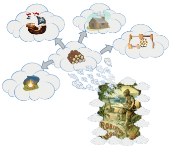
Figure 1: A castaway meditates on the optimal allocation of wood logs into several useful tasks such as: prepare a bonfire, build a ship, make a house or provide a fold for his flock.

2 Resource theories in general

A quantum resource theory’s essential idea is to study quantum information processing under a restricted set of physical operations. The permissible operations are called free and because they do not cover all physical processes that quantum mechanics allows only certain physically realizable objects of a quantum system can be prepared. Likewise, these accessible objects are called free, and any objects that are not free are called a resource. Thus a quantum resource theory identifies every physical process as being either free or prohibited and similarly it classifies every quantum object as being either free or a resource. The theory of entanglement forms a representative example of a quantum resource theory. For two or more quantum systems, entanglement can be characterized as a resource when free operations are local quantum operations and classical communication (LOCC) and free objects are separable states.

Another important element of a resource theory is a function $\mathcal{M}$ that maps the objects considered by the resource theory into the non-negative real numbers. The function $\mathcal{M}$ must be non-increasing under the free operations i.e. a monotone and should be proportional to the advantage of using the object for some operational task.

Definition 1

(Resource theory) A quantum resource theory is defined by a triple $\{\mathcal{F},\mathcal{O},\mathcal{M}\}$ where $\mathcal{F}$ is the set of free objects under consideration, for instance quantum states or quantum operations, which forms a subset within the set $\mathcal{S}$ of all quantum objects. The set $\mathcal{O}$ of free operations contains functions $o:\mathcal{S}\rightarrow\mathcal{S}$ which preserve the set of free objects. A function $\mathcal{M}:\mathcal{S}\rightarrow[0,\infty+[$, monotone under the set of free operations and such that $\mathcal{M}(f)=0$ for all $f\in\mathcal{F}$. The function $\mathcal{M}$ is said to measure the resourcefulness of objects in the set $\mathcal{S}$.

Because our research focuses on multipartite objects, we assume monotones $\mathcal{M}$ to be well defined when applied to every subsystem. The behaviour on multipartite objects of several standard measures, such as robustness, trace distance and entropic measures is already well known in the literature from the study of convertibility tasks, for more details see [3].

In the following we introduce the basic definitions of the resource theory of incompatibility which recently attracted the attention of the community [14, 15]. We will use this particular theory to illustrate the application of these definitions and show how they lead to sound but tractable optimization problems.

3 Resource theory of incompatibility

In quantum theory measurements are described by Positive Operator Value Measures (POVM). We define a POVM in dimension $d$ and a number of outcomes $n$ denoted by $\textbf{M}:=\{M_{1},M_{2},\ldots,M_{n}\}$ where each $M_{i}\in\mathcal{L}(\mathscr{H}_{d})$ is called measurement operator such that $M_{i}\geq 0$ and $\Sigma_{i}M_{i}=\textbf{I}$. Suppose a set of measurements $\{\textbf{M}_{x}\}_{x}$ where $x=1;...;m$, each described by measurement operators $M_{a|x}$ labels each of the measurement outcomes $a$ where $a=1,..,o$ such that $\Sigma_{a=1}^{o}M_{a|x}=\textbf{I}$ for every $x$. This set is said to be jointly measurable (or compatible) if there exists a parent POVM $\mathcal{G}$ with measurement operators $\mathcal{G}_{\lambda}$ and conditional probability distributions $p(a|x,\lambda)$ such that $M_{a|x}=\Sigma_{\lambda}p(a|x,\lambda)\mathcal{G}_{\lambda}$. Otherwise the set is said to be incompatible. One can introduce a resource-theoretic framework in the case of incompatibility with jointly measurable (compatible) POVM as a free measurement set $\mathcal{F}$ and the set of free operations $\mathcal{O}$ is: any single compatible measurement operator, classical post-processing and random mixing of single compatible measurements[14].

A recent important result shows that for every resourceful measurement $\mathbf{M}$ there is an instance of minimal-error quantum state discrimination game for which $\mathbf{M}$ gives greater success probability than all free measurements [16, 17, 18]. It has also been shown that the relative advantage of a resourceful measurement for state discrimination is proportional to the robustness measure [19, 20], which quantifies the minimal amount of noise that has to be added to a POVM to make it free. The formal expression for the generalized robustness of a measurement $\mathbf{M}$ is:

$$\mathcal{R}_{g}\left(\mathbf{M}\right)=\min\left\{s\in\mathbbm{R}_{\geq 0}\mid\exists\mathbf{N}\,\,\textrm{s.t.}\,\,\frac{\mathbf{M}+s\mathbf{N}}{1+s}\in\mathcal{F}\right\}$$ (1)

This is a monotone measure which means that for any measurement $\mathbf{M}$ and free operation $\phi\in\mathcal{O}$ we have $\mathcal{R}_{g}\left(\phi\left[\mathbf{M}\right]\right)\leq\mathcal{R}_{g}\left(\mathbf{M}\right)$. We use $\mathcal{R}_{g}$ in our work since it provides a clear operational interpretation of measurement incompatibility and is easy to define for any subsystem: simply choose any $\mathbf{N}$ that acts on the same systems as $\mathbf{M}$ such that the mixture is some compatible POVM on the corresponding systems.

4 Allocation of resources

The allocation of resources consists of distributing resources into a set of tasks according to a practical criterion, which usually involves optimizing a figure of merit. When the selected distribution method optimizes the figure of merit in the criteria, we have an optimal allocation of resources. We can see in Fig.1 a classic example of this problem, where an isolated man on an island must decide the best way to use the available resources.

In this article we restrict ourselves to study the above general problem in the case of multipartite quantum objects (a state $\rho$, a measurement $\mathbf{M}$ or a channel $\Xi$) denoted here by a common symbol $\sigma$. In a multipartite object, some subsets of the systems can be selected for different operational tasks. To describe this selection of relevant sets we shall use the notion of hypergraph $\mathcal{H}=\left\{\mathcal{V}_{\mathcal{H}},\mathcal{E}_{\mathcal{H}}\right\}$, in which hyperedges $\alpha\in\mathcal{E}_{\mathcal{H}}$ connect two or more vertices $v\in\mathcal{V}_{\mathcal{H}}$ [21]. We define a quantum resource allocation as the distribution of a quantum multipartite resource $\sigma$ over hypergraph $\mathcal{H}$ i.e. a list $\mathcal{A}_{\mathcal{H}}\left[\sigma\right]$ of values of the measure $\mathcal{M}$ applied to every reduction of $\sigma$ to parties in a hyperedge $\alpha$ of $\mathcal{H}$. The way in which the measure is applied for each $\alpha\in\mathcal{E}_{\mathcal{H}}$ must be specified in each case, which we exemplify later in our applications of our framework. To illustrate the concept of resource allocation we present hypergraphs $\mathcal{H}_{1}$, $\mathcal{H}_{2}$ and $\mathcal{H}_{3}$ in Fig.2 which have allocations:

$$\mathcal{A}_{\mathcal{H}_{1}}\left[\sigma_{abcd}\right] = \left\{\mathcal{M}\left(\sigma_{abcd}\right),\mathcal{M}\left(\textrm{Tr}_{d}\left(\sigma_{abcd}\right)\right)\right\}$$

$$\mathcal{A}_{\mathcal{H}_{2}}\left[\sigma_{ab}\right] = \left\{\mathcal{M}\left(\sigma_{ab}\right),\mathcal{M}\left(\textrm{Tr}_{a}\left(\sigma_{ab}\right)\right),\mathcal{M}\left(\textrm{Tr}_{b}\left(\sigma_{ab}\right)\right)\right\}$$

$$\mathcal{A}_{\mathcal{H}_{3}}\left[\sigma_{ab}\right] = \left\{\mathcal{M}\left(\sigma_{ab}\right),\mathcal{M}\left(\textrm{Tr}_{a}\left(\sigma_{ab}\right)\right)\right\}$$

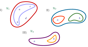
Figure 2: Examples of Hypergraphs used to determine the relevant parts of the resource allocation. Explicitly, the corresponding sets of hyperedges are $\mathcal{E}_{\mathcal{H}_{1}}=\left\{\left\{a,b,c,d\right\},\left\{a,b,c\right\}\right\}$, $\mathcal{E}_{\mathcal{H}_{2}}=\left\{\left\{a,b\right\},\left\{a\right\},\left\{b\right\}\right\}$ and $\mathcal{E}_{\mathcal{H}_{3}}=\left\{\left\{a,b\right\},\left\{b\right\}\right\}$.

If the list $\mathcal{A}_{\mathcal{H}}$ satisfies an optimality criterion $\mathscr{C}$ then we will say that the quantum resource allocation is optimal. The relevant criterion $\mathscr{C}$ depends on the allocation features we wish to optimize. If a task can be carried out by parts of the entire system specified by a hypergraph $\mathcal{H}$, then the performance $\Phi_{\mathscr{C}}$ of the allocation is given by a sum over hyperedges $\alpha\in\mathcal{E}_{\mathcal{H}}$ [8, 9]:

$$\Phi_{\mathscr{C}}\left(\mathcal{A}_{\mathcal{H}}\left[\sigma\right]\right)=\sum_{\alpha\in\mathcal{E}_{\mathcal{H}}}\Phi_{\mathscr{C},\alpha}\left(\mathcal{M}\left(\sigma_{\alpha}\right)\right)$$ (2)

Here $\Phi_{\mathscr{C},\alpha}:\mathbbm{R}_{\geq 0}\rightarrow\mathbbm{R}$ is some monotone function of the amount of resource allocated in hyperedge $\alpha$ and $\sigma_{\alpha}$ is the reduction of $\sigma$ in which the complement of $\alpha$ has been traced out. The properties of $\Phi_{\mathscr{C},\alpha}$ depend on how the allocation of resources at $\alpha$ contribute to the satisfaction of criterion $\mathscr{C}$. Since the operational task has associated the resource measure $\mathcal{M}$, the optimization problem consist in finding the multipartite resource $\sigma$ such that $\mathcal{A}_{\mathcal{H}}\left[\sigma\right]$ maximizes $\Phi_{\mathscr{C}}$ when $\mathcal{H}$ is fixed. The first optimality criterion $\mathscr{C}_{1}$ we will consider is the optimal proportional fairness criteria.This criterion is required when it is essential to allocate resources fairly among the parties. For example, these include allocation of bandwidth in telecommunication networks, takeoff and landing slots at airports, and water resources. For this case we maximize the performance of proportional fairness $\Phi_{\mathscr{C}_{1}}$ given by:

$$\Phi_{\mathscr{C}_{1}}\left(\mathcal{A}_{\mathcal{H}}\left[\sigma\right]\right)=\sum_{\alpha\in\mathcal{E}_{\mathcal{H}}}\log\left(\mathcal{M}\left(\sigma_{\alpha}\right)\right).$$ (3)

Hence, each $\Phi_{\mathscr{C}_{1},\alpha}\left(\cdot\right)$ is equal to $\log\left(\cdot\right)$. The choice $\Phi_{\mathscr{C}_{1},\alpha}\left(\cdot\right)=\log\left(\cdot\right)$ is useful in the case when no set of parts $\alpha$ has priority over others for the task performed [8]. In the case when certain priority order of the $\alpha\in\mathcal{E}_{\mathcal{H}}$ exists, a different figure of merit is used to ensure equitability [8] and we will discuss it later in the article. For example, the figure of merit $\Phi_{\mathscr{C}_{1}}$ is applied when in a communication network each demand is routed on a specified single path. From a resource point of view, the objective is to provide a resource $\sigma_{\alpha}$ to parties in the set $\alpha$ to communicate with an additional party $e\notin\mathcal{V}_{\mathcal{H}}$ in a way as fair as possible among all $\alpha\in\mathcal{E}_{\mathcal{H}}$. It can be shown that the optimal solution $\mathcal{A}_{\mathcal{H}}\left[\sigma^{\ast}\right]$ satisfies:

$$\sum_{\alpha\in\mathcal{E}_{\mathcal{H}}}\left(\frac{\mathcal{M}\left(\sigma_{\alpha}\right)-\mathcal{M}\left(\sigma_{\alpha}^{\ast}\right)}{\mathcal{M}\left(\sigma_{\alpha}\right)}\right)\leq 0$$

for every other $\mathcal{A}_{\mathcal{H}}\left[\sigma\right]$. Precisely, the solution $\mathcal{A}_{\mathcal{H}}\left[\sigma^{\ast}\right]$ is called proportionally fair since the aggregate of proportional changes with respect to any other feasible solution is zero or negative [8].

Next, we consider the optimal reliability criterion $\mathscr{C}_{2}$ which determines an optimal performance for a task in the presence of failures of the devices used by any one of its parts in each $\alpha\in\mathcal{E}_{\mathcal{H}}$. The appropriate performance $\Phi_{\mathscr{C}_{2}}$ which we maximize in this case reads:

$$\Phi_{\mathscr{C}_{2}}\left(\mathcal{A}_{\mathcal{H}}\left[\sigma\right]\right)=\sum_{\alpha\in\mathcal{E}_{\mathcal{H}}}\pi_{\alpha}\mathcal{M}\left(\sigma_{\alpha}\right),$$ (4)

where $\pi_{\alpha}$ denotes the prior probability that only parts in $\alpha$ will perform the task for which $\sigma$ is the resource. If every part $\left\{a_{1},\ldots,a_{n}\right\}$ has a prior chance $p_{a_{k}}$to work, then:

$$\pi_{\alpha}=\prod_{a_{i}\in\alpha}p_{a_{i}}\prod_{a_{j}\notin\alpha}\left(1-p_{a_{j}}\right).$$ (5)

The problem of optimal reliability is a relevant problem for different engineering areas which is usually addressed by redundacy models [9]. In (4) we adapt the classical performance function to fit the scheme of resource theories (see for instance the classical definition in section 1.23 in [9]) by choosing the $\Phi_{\mathscr{C}_{2},\alpha}\left(\cdot\right)$ to be the probability of successful performace only of parts in $\alpha$ rather than probability of failure, because $\mathcal{M}\left(\sigma_{\alpha}\right)$ is a measure of advantage provided by $\sigma_{\alpha}$ to the corresponding task.

The previous examples of performance and optimal reliability considered the case of a resource that should be shared in an optimal way among parties performing the same task. It should be noted that in principle one can define different tasks for each set $\alpha\in\mathcal{E}_{\mathcal{H}}$ in the two previous allocation problems. However, as we shall see on the following examples, the natural cases that involve multiple tasks are those where the availability of the resource is limited and - what is even more important - competition between the tasks exist. To describe such a situation in our notation consider for every resource $\sigma$ and all $\alpha\in\mathcal{E}_{\mathcal{H}}$:

$$\sum_{\alpha\in\mathcal{E}_{\mathcal{H}}}\Lambda_{\alpha}\left(\sigma\right)\mathcal{M}_{\alpha}\left(\sigma_{\alpha}\right) \leq \Gamma\left(\sigma\right)\>$$ (6)

$$L_{\alpha}\leq\mathcal{M}_{\alpha}\left(\sigma_{\alpha}\right) \leq U_{\alpha}\>.$$ (7)

with $\Lambda_{\alpha}\left(\sigma\right),\Gamma\left(\sigma\right)$ real non-negative functions of states and $L_{\alpha},U_{\alpha}$ some non-negative constants. Here we use explicitly the index dependence to express the possibility that the parties in each $\alpha\in\mathcal{E}_{\mathcal{H}}$ measure the resourcefulness of their $\sigma_{\alpha}$ with a different $\mathcal{M}_{\alpha}$. The choice of each $\mathcal{M}_{\alpha}$ is determined by the task assigned to the resource in each $\alpha$. The equations (6) stand for the trade-offs between the resources assigned for tasks at different $\alpha$ while the (7) determine prior limitations of the resources for each task. This set of inequalities is known as knapsack constraints (KC) [8]. In the case of two or more tasks involved and non-trivial knapsack constraints a typical optimality criterion $\mathscr{C}_{3}$ is the optimal equitability which is defined by a recursive max-min algorithm:

1. If upperbounds $U_{\alpha_{i}}\leq U_{\alpha_{j}}$ then introduce the condition $\mathcal{M}_{\alpha_{i}}\left(\sigma_{\alpha_{i}}\right)\leq\mathcal{M}_{\alpha_{j}}\left(\sigma_{\alpha_{j}}\right)$. The corresponding partial order determines the minimization over $\alpha\in\mathcal{E}_{\mathcal{H}}$ in the following steps.

2. If $\mathcal{\mathcal{E}_{\mathcal{H}}}\neq\left\{\emptyset\right\}$ then find a solution with prior KC for

   $$\Phi_{\mathscr{C}_{3}}\left(\mathcal{A}_{\mathcal{H}}\left[\sigma\right]\right)=\sup_{\sigma}\min_{\alpha\in\mathcal{E}_{\mathcal{H}}}\mathcal{M}_{\alpha}\left(\sigma_{\alpha}\right)$$

3. Let us call $\alpha_{1}$ the $\alpha\in\mathcal{E}_{\mathcal{H}}$ such that $\mathcal{M}_{\alpha_{1}}\left(\sigma_{\alpha_{1}}\right)$ is the minimum on step 1. If $\mathcal{E}_{\mathcal{H}}/\alpha_{1}=\mathcal{E}_{\mathcal{H}}^{(1)}\neq\left\{\emptyset\right\}$ then find a solution with prior KC for:

   $$\Phi_{\mathscr{C}_{3}}\left(\mathcal{A}_{\mathcal{H}^{(1)}}\left[\sigma\right]\right)=\sup_{\sigma}\min_{\alpha\in\mathcal{E}_{\mathcal{H}}^{(1)}}\mathcal{M}_{\alpha}\left(\sigma_{\alpha}\right)$$

   under the additional constraint:

   $$\Phi_{\mathscr{C}_{3}}\left(\mathcal{A}_{\mathcal{H}}\left[\sigma\right]\right)=\mathcal{M}_{\alpha_{1}}\left(\sigma_{\alpha_{1}}\right)\leq\mathcal{M}_{\alpha}\left(\sigma_{\alpha}\right)$$

   for all $\alpha\in\mathcal{E}_{\mathcal{H}}^{(1)}$.

4. Iterate with corresponding $\alpha_{n-1}$ from $\alpha\in\mathcal{E}_{\mathcal{H}}^{(n-2)}$ such that $\mathcal{M}_{\alpha_{n-1}}\left(\sigma_{\alpha_{n-1}}\right)$ is the minimum on step $n-1$. If $\mathcal{E}_{\mathcal{H}}^{(n-2)}/\alpha_{n-1}=\mathcal{\mathcal{E}_{\mathcal{H}}}^{(n-1)}\neq\left\{\emptyset\right\}$ then find a solution with prior KC for

   $$\Phi_{\mathscr{C}_{3}}\left(\mathcal{A}_{\mathcal{H}^{(n-2)}}\left[\sigma\right]\right)=\sup_{\sigma}\min_{\alpha\in\mathcal{E}_{\mathcal{H}}^{(n-1)}}\mathcal{M}_{\alpha}\left(\sigma_{\alpha}\right)$$

   under the additional constraints:

   $$\mathcal{M}_{\alpha_{1}}\left(\sigma_{\alpha_{1}}\right)\leq...\leq\mathcal{M}_{\alpha_{n-1}}\left(\sigma_{\alpha_{n-1}}\right)\leq\mathcal{M}_{\alpha}\left(\sigma_{\alpha}\right)$$

   for all $\alpha\in\mathcal{E}_{\mathcal{H}}^{(n-1)}$ and such that:

   $$\Phi_{\mathscr{C}_{3}}\left(\mathcal{A}_{\mathcal{H}^{\left(m-1\right)}}\left[\sigma\right]\right)=\mathcal{M}_{\alpha_{m}}\left(\sigma_{\alpha_{m}}\right)$$

   for each $\mathcal{M}_{\alpha_{m}}\left(\sigma_{\alpha_{m}}\right)$.

5. When $\mathcal{E}_{\mathcal{H}}^{(m-1)}=\left\{\emptyset\right\}$ stop.

In the previous recursive algorithm minimization of $\mathcal{M}_{\alpha}\left(\sigma_{\alpha}\right)$ over $\alpha\in\mathcal{E}_{\mathcal{H}}$ considers $\mathcal{M}_{\alpha_{i}}\left(\sigma_{\alpha_{i}}\right)\leq\mathcal{M}_{\alpha_{j}}\left(\sigma_{\alpha_{j}}\right)$ iff $U_{\alpha_{i}}\leq U_{\alpha_{j}}$ because in this case allocating resources in $\alpha_{j}$ is potentially more advantageous than in $\alpha_{i}$. We also note that the above algorithm will halt in finite number steps because the number of $\alpha\in\mathcal{\mathcal{E}_{\mathcal{H}}}$ is finite. Solutions to optimal equitability are known to be non-unique, but nevertheless they provide a set of solutions considered safe for the usual practical applications [8]. If this is not satisfactory, a unique solution can be ensured by additional requirements such as Pareto optimality [8] of the final order $\mathcal{M}_{\alpha_{1}}\left(\sigma_{\alpha_{1}}\right)\leq...\leq\mathcal{M}_{\alpha_{N}}\left(\sigma_{\alpha_{N}}\right)$.

It is essential to highlight that the theoretical framework we developed for the allocation of quantum resources is entirely general and that it is possible to apply it in any case that requires at least two agents performing more than one instance of a task or more than one task with their quantum devices. That said, the next section’s results illustrate the usefulness of the theoretical framework by demonstrating concrete and relevant applications.

5 Results

5.1 Fair and reliable allocation of incompatible measurements

Before presenting a specific example of resource allocation let us recall the notion of unbiased bases. Two orthogonal measurements with labels $j,j^{\prime}\in\left\{0,1\right\}$ are unbiased iff they satisfy the following condition:

$$\left|\left\langle u_{a}^{j}\mid u_{b}^{j^{\prime}}\right\rangle\right|^{2}=\begin{cases}\delta_{ab}&;\,j=j^{\prime}\\ \frac{1}{D}&;\,j\neq j^{\prime}\end{cases}$$ (8)

where $D$ is the total dimension of the system [22, 23]. Two unbiased bases consisting of product states only were introduced in [24], for which case we write $\left|u_{\mathbf{a}}^{x}\right\rangle=\left|u_{a_{1}}^{x}\right\rangle\otimes\ldots\otimes\left|u_{a_{N}}^{x}\right\rangle$ with each $\left|u_{a_{k}}^{x}\right\rangle$ a state from two unbiased bases. Therefore, for $N$ systems of dimension $d$ two product unbiased measurements $\left|u_{\mathbf{a}}^{x_{1}}\right\rangle\left\langle u_{\mathbf{a}}^{x_{1}}\right|,\left|u_{\mathbf{b}}^{x_{2}}\right\rangle\left\langle u_{\mathbf{b}}^{x_{2}}\right|$ satisfy (8) replacing $\delta_{ab}\rightarrow\delta_{\mathbf{ab}}$ and $D=d^{N}$. It was demonstrated in [24] that one can find at least two product bases in $\mathscr{H}_{d}^{\otimes N}$ which are mutually unbiased and such that any of their reductions to $M$ qudits forms a set of two unbiased product bases in $\mathscr{H}_{d}^{\otimes M}$. The above property demonstrates that product unbiased bases form a nested measurement (in the sense of [25]), which means that tracing out any of the parts of the POVMs the remaining measurements are also product unbiased bases.

Our main contribution consists of two examples that demonstrate the optimal allocation of quantum resources to be sound and tractable problems. Indeed, in our first example we show an explicit POVM $\widetilde{\mathbf{M}}=\left\{\widetilde{M}_{x}\right\}_{x}$ for which the allocation $\mathcal{A}_{\mathcal{H}}\left[\widetilde{\mathbf{M}}\right]$ satisfies both optimality criteria $\mathscr{C}_{1}$ and $\mathscr{C}_{2}$ for any $\mathcal{H}$ of qudits in the resource theory of incompatible measurements. The elements of each $\widetilde{M}_{x}$ are given by the projectors $\left|u_{\mathbf{a}}^{x=1}\right\rangle\left\langle u_{\mathbf{a}}^{x=1}\right|,\left|u_{\mathbf{b}}^{x=2}\right\rangle\left\langle u_{\mathbf{b}}^{x=2}\right|$, onto the unbiased bases. Then we arrive at the following theorem:

Theorem 1

Consider an optimal allocation with arbitrary hypergraph $\mathcal{H}$ of a given measurement $\mathbf{M}$ over a number $N$ of qudits of dimension $d$ and with optimality criterion $\mathscr{C}$. If the criterion $\mathscr{C}$ requires maximization of performance function $\Phi_{\mathscr{C}}$, with allocation $\mathcal{A}_{\mathcal{H}}\left[\mathbf{M}\right]=\left\{\mathcal{R}_{g}\left(\mathbf{M}_{\alpha}\right)\right\}_{\alpha\in\mathcal{E}_{\mathcal{H}}}$ defined by the generalized robustness $\mathcal{R}_{g}$, then the measurement $\widetilde{\mathbf{M}}$ composed of two product unbiased bases is a feasible optimal solution in the resource theory of incompatibility.

Proof: First, we need to specify in which way $\mathcal{R}_{g}$ applies to every possible measurement $\mathbf{M}_{\alpha}$ indexed by the hyperedge $\alpha$ of the hypergraph. We use equation (1) specified to the measurement $\mathbf{M}_{\alpha}$, where the mixture $(\mathbf{M}_{\alpha}+s\mathbf{N}_{\alpha})/(1+s)$ belongs to the set $\mathcal{F}_{\alpha}$ of compatible measurements only on the composed system $\alpha\in\mathcal{E}_{\mathcal{H}}$ and $\mathbf{N}_{\alpha}$ is some measurement also on the systems in $\alpha$. This $\alpha$-wise application of $\mathcal{M}_{g}$ is meaningful since it should measure the advantage of $\mathbf{M}_{\alpha}$ over any compatible measurement of parties in $\alpha\in\mathcal{E}_{\mathcal{H}}$. Now, we remark the recent proof in [15] that unbiased bases are optimal incompatible measurements under the generalized robustness monotone $\mathcal{R}_{g}$ in any dimension $d$. Since, we can always find two product unbiased bases to define $\widetilde{\mathbf{M}}$, then because product unbiased bases are nested measurements the evaluation of $\mathcal{R}_{g}$ for each $\alpha\in\mathcal{\mathcal{E}_{\mathcal{H}}}$ yields the maximal value, hence for any monotone function $\Phi_{\mathscr{C}}$ of $\mathcal{A}_{\mathcal{H}}\left[\widetilde{\mathbf{M}}\right]=\left\{\mathcal{R}_{g}\left(\widetilde{\mathbf{M}}_{\alpha}\right)\right\}_{\alpha\in\mathcal{E}_{\mathcal{H}}}$ – such as $\Phi_{\mathscr{C}_{1}}$ or $\Phi_{\mathscr{C}_{2}}$– the $\widetilde{\mathbf{M}}$ measurement achieves the maximal value q.e.d.

As an Illustration, we present optimal allocations associated with the hypergraphs from Fig.2. The maximal value $\Phi_{\mathscr{C}_{1}}^{max}$ achieved by $\Phi_{\mathscr{C}_{1}}\left(\mathcal{A}_{\mathcal{H}_{1}}\left[\widetilde{\mathbf{M}}\right]\right)$ is:

$$\Phi_{\mathscr{C}_{1}}^{max}=\log\left(\frac{d^{2}-1}{d^{2}+1}\right)+\log\left(\frac{d^{3/2}-1}{d^{3/2}+1}\right)$$ (9)

Another example is the maximal value $\Phi_{\mathscr{C}_{2}}^{max}$ achieved by $\Phi_{\mathscr{C}_{2}}\left(\mathcal{A}_{\mathcal{H}_{2}}\left[\widetilde{\mathbf{M}}\right]\right)$ for each qudit pair of dimension $d$ is:

$$\Phi_{\mathscr{C}_{2}}^{max}=\pi_{\left\{a,b\right\}}\left(\frac{d-1}{d+1}\right)+\left(\pi_{\left\{a\right\}}+\pi_{\left\{b\right\}}\right)\left(\frac{\sqrt{d}-1}{\sqrt{d}+1}\right)$$ (10)

Since the resources in this particular resource theory are advantageous for state discrimination, our result shows that the device which implements the optimal measurement $\widetilde{\mathbf{M}}$ also has optimal performance for such a task in the presence of failures of any subsystem. The scenario represented by $\mathcal{H}_{2}$ is the simplest case in which “at most a number $K$ of devices may fail”, which defines a problem of allocation relevant to the performance of different engineering tasks [9].

5.2 Equitable allocation of nonlocality versus local contextuality

The equitability criterion described in section 4 is relevant in contexts where there is some trade-off between resources distributed among agents. Such contexts are not strange in quantum information, for example, we can mention some cases such as extracting work from local states [26] versus obtaining thermodynamic work from shared correlations [27, 28] or obtaining random local states [29] versus sharing private bit states [30]. For the tasks mentioned above, the cited articles quantify the appropriate resources with monotones based on entropic measures to which our theoretical framework applies. However, below we select cases of nonlocality versus local contextuality trade-offs due to their simplicity. Our choice of a specific case allows us to present a proof of concepts clearly and understandably.

Nonlocality and contextuality, are well known resources for communication and randomness amplification tasks [31, 32, 33, 34, 35]. A monotone for these state resource theories is [35, 34]:

$$\mathcal{N}\left(\rho\right)=\sup_{\phi\in\Phi}\mathcal{I}\left(\phi\left[\rho\right]\right)-\mathcal{B}_{c}$$ (11)

where $\mathcal{I}$ is the Bell correlation function, $\Phi$ is the set of free operations (see Appendix A) and $\mathcal{B}_{c}$ is the classical bound. We will use the resource theories of nonlocality and contextuality to exemplify a resource scenario in which the optimal equitability criteria $\mathscr{C}_{3}$ is useful. In this scenario, a hypergraph $\mathcal{H}_{3}:\>\mathcal{V}_{\mathcal{H}_{3}}=\left\{a,b\right\},\mathcal{E}_{\mathcal{H}_{3}}=\left\{\left\{a,b\right\},\left\{b\right\}\right\}$ defines the allocation of the resource state $\rho$. The objective of party $b$ is to perform a task that improves with the contextuality of his local state $\rho_{b}=\textrm{Tr}_{a}\left(\rho\right)$, while parties $a,b$ should perform a task that requires nonlocality of their bipartite state $\rho_{a,b}=\rho$.

For our application of $\mathscr{C}_{3}$ is important the existence of a fundamental trade-off between both resources [36] :

$$\mathcal{I}_{n}\left(\rho\right)+\mathcal{I}_{m}\left(\rho\right)\leq n+m-4$$ (12)

Here $\mathcal{I}_{s}\left(\rho\right)$ stands for a cyclic correlation,

$$\mathcal{I}_{s}\left(\rho\right)=\sum_{k=1}^{s-1}\left\langle B_{k}B_{k+1}\right\rangle_{\rho}-\left\langle B_{s}B_{1}\right\rangle_{\rho},$$ (13)

where the average of observable $O=\left\{O_{k}\right\}_{k}$ given by $\left\langle O\right\rangle_{\rho}=\sum_{k}o_{k}Tr\left(O_{k}\rho\right)$, with $o_{k}\in\{-1,+1\}$ the numerical value of $O$ associated with $O_{k}$ and $\mathcal{B}_{c}^{s}=s-2$ is the classical bound. The correlation $\mathcal{I}_{s}\left(\rho\right)$ witnesses nonlocality or contextuality depending on the kind of constraints satisfied by the $\left\{B_{1},...,B_{s}\right\}$ observables [36]. Then, if we replace appropriately $\mathcal{I}_{s}$ and $\mathcal{B}_{c}^{s}$ in (11) to define a monotone $\mathcal{N}_{s}\left(\rho\right)$ the inequality (12) implies the resource relation:

$$\Lambda_{n}\left(\rho_{a,b}\right) \mathcal{N}_{n}\left(\rho_{a,b}\right)+\Lambda_{m}\left(\rho_{b}\right)\mathcal{N}_{m}\left(\rho_{b}\right)\leq...$$

$$\Lambda_{n}\left(\rho_{a,b}\right) \left[\mathcal{B}_{Q}^{n}-\mathcal{B}_{c}^{n}\right]+\Lambda_{m}\left(\rho_{b}\right)\left[\mathcal{B}_{Q}^{m}-\mathcal{B}_{c}^{m}\right]\,\,\,$$

$$\Lambda_{s}\left(\rho_{\alpha}\right) =\frac{1+\textrm{sgn}\left(\mathcal{I}_{s}\left(\rho_{\alpha}\right)-\mathcal{B}_{c}^{s}\right)}{2}$$

with $\mathcal{B}_{Q}^{s}$ is the quantum Tsirelson bound (i.e. quantumly saturable) for $\mathcal{I}_{s}\left(\rho\right)$ and $\textrm{sgn}(\cdot)$ the sign function. From an allocation of resources perspective the inequality (5.2) defines a knapsack constraint like (6). The individual bounds (7) correspond here to $\mathcal{N}_{n}(\rho_{a,b})\leq\mathcal{B}^{n}_{Q}-\mathcal{B}^{n}_{c}$ and $\mathcal{N}_{m}(\rho_{b})\leq\mathcal{B}^{m}_{Q}-\mathcal{B}^{m}_{c}$ respectively. The optimal equitable solutions in this case are simply:

Solution 1: $$\left\{\begin{array}[]{c}\mathcal{N}_{n}\left(\rho_{a,b}\right)=\mathcal{B}_{Q}^{n}-\mathcal{B}_{c}^{n}\\ \\ \mathcal{N}_{m}\left(\rho_{b}\right)=0\end{array}\right.$$

Solution 2: $$\left\{\begin{array}[]{c}\mathcal{N}_{n}\left(\rho_{a,b}\right)=0\\ \\ \mathcal{N}_{m}\left(\rho_{b}\right)=\mathcal{B}_{Q}^{m}-\mathcal{B}_{c}^{m}\end{array}\right.$$

If $\mathcal{B}_{Q}^{n}-\mathcal{B}_{c}^{n}>\mathcal{B}_{Q}^{m}-\mathcal{B}_{c}^{m}$ then the max-min algorithm will select Solution 1, since in this case $\mathcal{N}_{n}\left(\rho_{a,b}\right)>\mathcal{N}_{m}\left(\rho_{b}\right)$ is the choice that maximizes the overall amount of resources provided by $\rho$. Conversely if $\mathcal{B}_{Q}^{n}-\mathcal{B}_{c}^{n}<\mathcal{B}_{Q}^{m}-\mathcal{B}_{c}^{m}$ we will obtain Solution 2 and finally, if $\mathcal{B}_{Q}^{n}-\mathcal{B}_{c}^{n}=\mathcal{B}_{Q}^{m}-\mathcal{B}_{c}^{m}$ both solution are acceptable, if only equitability is demanded.

A nontrivial scenario for optimal equitability arises in the case of monogamy activation, for example in the following relationship [36]:

$$\mathcal{I}_{A}^{B}\left(\rho_{a,b}\right)+\mathcal{I}_{C}^{B}\left(\rho_{b,c}\right)+2\mathcal{I}_{5}\left(\rho_{b}\right)\leq 14$$ (17)

Here, $\mathcal{I}_{5}\left(\rho_{b}\right)$ is a contextual cycle correlation with $B_{k}$ observables as in (13), while $\mathcal{I}_{A}^{B}\left(\rho_{a,b}\right),\mathcal{I}_{C}^{B}\left(\rho_{b,c}\right)$ stand for $I_{3322}$ inequalities [36]:

$$\mathcal{I}_{A}^{B}\left(\rho_{a,b}\right)=\left\langle B_{1}\right\rangle_{\rho}+\left\langle B_{4}\right\rangle_{\rho}+\left\langle A_{1}\right\rangle_{\rho}+\left\langle A_{2}\right\rangle_{\rho}-\left\langle B_{1}A_{1}\right\rangle_{\rho}\\ -\left\langle B_{1}A_{2}\right\rangle_{\rho}-\left\langle B_{1}A_{3}\right\rangle_{\rho}-\left\langle B_{4}A_{1}\right\rangle_{\rho}-\left\langle B_{4}A_{2}\right\rangle_{\rho}\\ +\left\langle B_{4}A_{3}\right\rangle_{\rho}-\left\langle B_{6}A_{1}\right\rangle_{\rho}+\left\langle B_{6}A_{2}\right\rangle_{\rho}\leq 4$$ (18)

and analogously for $\mathcal{I}_{C}^{B}\left(\rho_{b,c}\right)$ by replacing each $A_{k}$ by $C_{k}$. Now, we study the allocation scenario defined by $\mathcal{H}_{3}$, and with operational tasks associated with $\mathcal{I}_{A}^{B}\left(\rho_{a,b}\right)$ and $\mathcal{I}_{5}\left(\rho_{b}\right)$. In this case we assume $\rho_{b,c}$ to be resourceless, but with a fixed value $\mathcal{I}_{C}^{B}\left(\rho_{b,c}\right)=\lambda<4$. Then, we can state an equitability problem defined by the constraints:

$$\mathcal{N}_{A}^{B}\left(\rho_{a,b}\right)+2\mathcal{N}_{5}\left(\rho_{b}\right) \leq 4-\lambda$$

$$0\leq\mathcal{N}_{A}^{B}\left(\rho_{a,b}\right) \leq \mathcal{B}_{Q}^{\gamma}-4$$

$$0\leq\mathcal{N}_{5}\left(\rho_{b}\right) \leq \mathcal{B}_{Q}^{5}-3$$ (19)

The monotones $\mathcal{N}_{A}^{B}\left(\rho_{a,b}\right)$ and $\mathcal{N}_{5}\left(\rho_{b}\right)$ are defined analogously as $\mathcal{N}_{s}\left(\rho\right)$ in (11), and $\mathcal{B}_{Q}^{\gamma}$, $\mathcal{B}_{Q}^{5}$ are the quantum bounds for $I_{3322}$ and $\mathcal{I}_{5}\left(\rho\right)$ respectively. In this case the solution is nontrivial and reads:

Solution 3: $$\left\{\begin{array}[]{c}\mathcal{N}_{A}^{B}\left(\rho_{a,b}\right)=\frac{\mu}{3}\\ \\ \mathcal{N}_{5}\left(\rho_{b}\right)=\frac{\mu}{3}\end{array}\right.$$ (23)

with $\mu=4-\lambda$ (for the proof see Appendix A, section A.2). As mentioned before, nonlocal and contextual resources are useful for randomness amplification [31, 32]. Therefore, an application of the solutions to the problems presented is an equitable assignment of security into quantum networks. In consequence, the above examples show that optimal equitable allocations of resources are relevant for concrete tasks in quantum information.

6 Discussion

In quantum information, a variety of approaches are used to determine the practical value of quantum systems, such as cryptography, communication capacity, computational complexity and thermodynamics. The common factor among these approaches is the search for quantum resources to benefit agents in performing specific tasks. Observed as a whole, these form an economy that requires tools to manage such quantum resources, optimal allocation being crucial.

This article applies three different criteria of the optimal allocation of quantum resources and demonstrates solutions to the corresponding optimization problems. We propose the above results for applications in the interplay between quantum processing machines (computers) and a quantum communication network (see [37, 38, 39]).

Indeed, our results contribute to the line of work proposed by S. Wehner et al. [40] for developing the Quantum Internet in six functionality driven stages. Precisely, Theorem 1 shows that there are multipartite quantum resources for communication tasks in prepare-and-measure networks with the optimally proportionally fair and reliable distribution. Such a result fits the type of advances desired for quantum networks in the second functionality stage of the Quantum Internet.

Furthermore, our example of the optimal equitability criteria may be a starting point for analyzing network scenarios in the third stage proposed for Quantum Internet development (Entanglement distribution networks [40]). Indeed, nonlocality may be a self-testing benchmark for entanglement while contextuality may be related to coherence. The former may be related to communication between the nodes, and the latter - to quantum information processing at the nodes. If we have limited fault-tolerant resources for protecting both local and nonlocal quantumness, then the optimal equitability may help find a balance between local computation and delegation of tasks, especially if desired to be secure (see [41]). Independently the very nonlocality at single computing node may be one day an important resource itself (see [42]). We leave these and related topics for further research.

In addition, the scheme we present opens the possibility of finding applications for multi-party systems that nest resources symmetrically [43]. In this sense, our results suggest that resource nesting may be potentially a tool for distributing resources according to specific criteria relevant to the corresponding tasks.

In conclusion, it seems natural to expect that quantum resources will need soon the tools to allocate resources provided in this article. It may be helpful at the level of designing quantum information processing protocols (or - possibly - even some practical experiments with limited quantum coherence effects). On the other hand, the methods and tools for allocating resources can contribute to the theoretical analysis of trade-offs between different quantum information resources. One can even expect that they can contribute to developing some form of the economy of quantum resources. The administration of quantum networks – such as the Quantum Internet – could be one of this new economy’s first challenge.

7 Acknowledgements

RS, TB and PH acknowledge support by the Foundation for Polish Science (IRAP project, ICTQT, contract no.2018/MAB/5, co-financed by EU within Smart Growth Operational Programme). JC and KZ thank the support of National Science Center in Poland under the grant numbers DEC-2019/35/O/ST2/01049 and DEC-2015/18/A/ST2/00274 and by Foundation for Polish Science under the grant TEAM-NET project (contract no. POIR.04.04.00-00-17C1/18-00). We also thank A. de Oliveira Junior, Debashis Saha and Gabriel Muniz for advice and help with the design of figures.

Appendix A Appendix

A.1 Resource theories of nonlocality and contextuality

The resource theories of nonlocality and contextuality usually consider as objects boxes with at least two integer inputs $x_{1},x_{2}$ and two integer outputs $a_{1},a_{2}$, which are characterized by the conditional probabilities $P\left(a_{1},a_{2}\mid x_{1},x_{2}\right)$ called behaviours [34, 35]. In our research we consider only quantum resources, hence every behaviour can be written as:

$$P\left(a_{1},a_{2}\mid x_{1},x_{2}\right)=Tr\left(\rho_{1,2}M_{a_{1}\mid x_{1}}^{\left(1\right)}\otimes M_{a_{2}\mid x_{2}}^{\left(2\right)}\right)$$ (24)

For a bipartite state $\rho_{1,2}$ and measurements $M_{a_{1}\mid x_{1}}^{\left(1\right)}\otimes M_{a_{2}\mid x_{2}}^{\left(2\right)}$ for systems $1,2$. Moreover, in each case we consider fixed measurements, such that in our study the resource theories of nonlocality and contextuality can as well be considered resource theories of quantum states. Because of this some examples of free operations for nonlocality and contextuality can be local operations as well mixing of states. If in both cases the set $\Phi$ is defined as the closure of free operations under composition, the measure $\mathcal{N}_{s}\left(\rho\right)$ defined in (11) is a monotone:

$$\mathcal{N}_{s}\left(\phi\left[\rho\right]\right)\leq\mathcal{N}_{s}\left(\rho\right)\>\forall\phi\in\Phi$$ (25)

due to the definition of supremum.

A.2 Non-trivial solutions of allocation in the monogamy activation scenario

Here we provide in more detail the possible equitable solutions to the problem with knapsack constraints (19). First, let’s define the auxiliary variables $\mu=4-\lambda$, $\nu_{1}=\mathcal{B}_{Q}^{I_{3322}}-4$ and $\nu_{2}=\mathcal{B}_{Q}^{5}-3$. In Appendix C we show that $\nu_{1}\geq 1$ and from reference [44] $v_{2}=0.9442$, hence $\nu_{1}>\nu_{2}.$ From the above and the partial order imposed by the equitability criteria $\mathscr{C}_{3}$ we have:

$$\mathcal{N}_{5}\left(\rho_{\left\{b\right\}}\right)\leq\mathcal{N}_{A}^{B}\left(\rho_{\left\{a,b\right\}}\right)$$ (26)

which means that in this scenario the advantage provided by nonlocality of $\rho_{\left\{a,b\right\}}$ is potentially greater than the noncontextuality of $\rho_{\left\{b\right\}}$, therefore has priority. Additionally we know (See ref [36, 44, 45]) that all values for $\mathcal{I}_{5}\left(\rho_{\left\{b\right\}}\right),\mathcal{I}_{A}^{B}\left(\rho_{\left\{a,b\right\}}\right),\lambda$ satisfying the trade-off (17) and Tsirelson bounds to be achievable for some $\rho_{a,b,c}$, then the supreme in each step of the optimal equitability criterion can be replaced by a maximization. Later, because the optimization is over a convex set – of $\mathcal{N}_{5}\left(\rho_{\left\{b\right\}}\right),\mathcal{N}_{A}^{B}\left(\rho_{a,b}\right)$– the solution must lie at a boundary. A solution in the boundary $\mathcal{N}_{5}\left(\rho_{\left\{b\right\}}\right)=\nu_{2}$ will violate the requirements (19) or (26) because $\mu\leq 2\nu_{2}$, on the other hand a solution with $\mathcal{N}_{A}^{B}\left(\rho_{\left\{a,b\right\}}\right)=\nu_{1}$, implies $\mathcal{N}_{5}\left(\rho_{\left\{b\right\}}\right)=0$ which is actually a minimum. Then, to find a maximum for $\mathcal{N}_{5}\left(\rho_{\left\{b\right\}}\right)$ under the constraints, we search at the boundary:

$$\mathcal{N}_{A}^{B}\left(\rho_{\left\{a,b\right\}}\right)+2\mathcal{N}_{5}\left(\rho_{\left\{b\right\}}\right) = \mu$$

$$\Rightarrow\mathcal{N}_{A}^{B}\left(\rho_{\left\{a,b\right\}}\right) = \mu-2\mathcal{N}_{5}\left(\rho_{\left\{b\right\}}\right)$$ (27)

Replacing (27) in (26) we obtain:

$$\mathcal{N}_{5}\left(\rho_{\left\{b\right\}}\right)\leq\frac{\mu}{3}<\nu_{2}$$ (28)

Since the lower bound of $\mathcal{N}_{A}^{B}\left(\rho_{\left\{a,b\right\}}\right)$ is zero, the maximum value that $\mathcal{N}_{5}\left(\rho_{\left\{b\right\}}\right)$ can achieve is $\mu/3$ in which case we have the equitable Solution 3 of main text. The solution (23) maximizes the amount of resources under constraints (19) and minimizes the difference between $\mathcal{N}_{A}^{B}\left(\rho_{\left\{a,b\right\}}\right)$ and $\mathcal{N}_{5}\left(\rho_{\left\{b\right\}}\right)$.

A.3 The quantum bound of $I_{3322}$

The Bell operator $\mathbbm{B}_{Q}^{v}$ of the $I_{3322}$ inequality was introduced in reference [45]:

$$\mathbbm{B}_{Q}^{v}=-A_{2}\otimes\mathbbm{I}-\mathbbm{I}\otimes B_{1}-2\mathbbm{I}\otimes B_{4}+A_{1}\otimes B_{1}$$

$$+A_{1}\otimes B_{4}+A_{2}\otimes B_{1}+A_{2}\otimes B_{4}-A_{1}\otimes B_{6}$$

$$+A_{2}\otimes B_{6}-A_{3}\otimes B_{1}+A_{3}\otimes B_{4}$$ (29)

in terms of binary operators $\left\{A_{1},A_{2},A_{3},B_{1},B_{4},B_{6}\right\}$ with outcomes $0$ and $1$,

$$A_{i} = (1)A_{i}^{1}+(0)A_{i}^{\perp}\>i\in\left\{1,2,3\right\}$$

$$B_{j} = (1)B_{j}^{1}+(0)B_{j}^{\perp}\>j\in\left\{1,4,6\right\}$$

However, in this article we use binary operators with outcomes $-1$ and $1$,

$$A_{i}^{\prime} = (1)A_{i}^{1}+(-1)A_{i}^{\perp}\>i\in\left\{1,2,3\right\}$$

$$B_{j}^{\prime} = (1)B_{j}^{1}+(-1)B_{j}^{\perp}\>j\in\left\{1,4,6\right\}$$

Then, in this appendix we will show how to transform $\mathbbm{B}_{Q}^{v}$ into an operator $\mathbbm{B}_{Q}^{\gamma}$ in terms of binary operators with outcomes $-1$ and $1$. First, note that:

$$A_{i}^{1}+A_{i}^{\perp} = \mathbbm{I}$$ (30)

$$B_{j}^{1}+B_{j}^{\perp} = \mathbbm{I}$$ (31)

for all $i\in\left\{1,2,3\right\}$ and $j\in\left\{1,4,6\right\}$ respectively. In consequence:

$$A_{i}=A_{i}^{1} = \frac{1}{2}\left(\mathbbm{I}+A_{i}^{\prime}\right)$$ (32)

$$B_{j}=B_{j}^{1} = \frac{1}{2}\left(\mathbbm{I}+B_{j}^{\prime}\right)$$ (33)

Second, we apply (32), (33) to replace each $A_{i}$ and $B_{j}$ in the definition of $\mathbbm{B}_{Q}^{v}$ we obtain:

$$\mathbbm{B}_{Q}^{v}=-\left(\frac{\mathbbm{I}\otimes\mathbbm{I}+A^{\prime}_{2}\otimes\mathbbm{I}}{2}\right)-\left(\frac{\mathbbm{I}\otimes\mathbbm{I}+\mathbbm{I}\otimes B^{\prime}_{1}}{2}\right)$$

$$-2\left(\frac{\mathbbm{I}\otimes\mathbbm{I}+\mathbbm{I}\otimes B^{\prime}_{4}}{2}\right)+\left(\frac{\mathbbm{I}\otimes\mathbbm{I}+A^{\prime}_{1}\otimes\mathbbm{I}+\mathbbm{I}\otimes B^{\prime}_{1}+A^{\prime}_{1}\otimes B^{\prime}_{1}}{4}\right)$$

$$+\left(\frac{\mathbbm{I}\otimes\mathbbm{I}+A^{\prime}_{1}\otimes\mathbbm{I}+\mathbbm{I}\otimes B^{\prime}_{4}+A^{\prime}_{1}\otimes B^{\prime}_{4}}{4}\right)+\left(\frac{\mathbbm{I}\otimes\mathbbm{I}+A^{\prime}_{2}\otimes\mathbbm{I}+\mathbbm{I}\otimes B^{\prime}_{1}+A^{\prime}_{2}\otimes B^{\prime}_{1}}{4}\right)$$

$$+\left(\frac{\mathbbm{I}\otimes\mathbbm{I}+A^{\prime}_{2}\otimes\mathbbm{I}+\mathbbm{I}\otimes B^{\prime}_{4}+A^{\prime}_{2}\otimes B^{\prime}_{4}}{4}\right)-\left(\frac{\mathbbm{I}\otimes\mathbbm{I}+A^{\prime}_{1}\otimes\mathbbm{I}+\mathbbm{I}\otimes B^{\prime}_{6}+A^{\prime}_{1}\otimes B^{\prime}_{6}}{4}\right)$$

$$+\left(\frac{\mathbbm{I}\otimes\mathbbm{I}+A^{\prime}_{2}\otimes\mathbbm{I}+\mathbbm{I}\otimes B^{\prime}_{6}+A^{\prime}_{2}\otimes B^{\prime}_{6}}{4}\right)-\left(\frac{\mathbbm{I}\otimes\mathbbm{I}+A^{\prime}_{3}\otimes\mathbbm{I}+\mathbbm{I}\otimes B^{\prime}_{1}+A^{\prime}_{3}\otimes B^{\prime}_{1}}{4}\right)$$

$$+\left(\frac{\mathbbm{I}\otimes\mathbbm{I}+A^{\prime}_{3}\otimes\mathbbm{I}+\mathbbm{I}\otimes B^{\prime}_{4}+A^{\prime}_{3}\otimes B^{\prime}_{4}}{4}\right)$$

After some algebraic simplifications we obtain:

$$4\mathbbm{B}_{Q}^{v}+4\mathbbm{I}\otimes\mathbbm{I}=A^{\prime}_{1}\otimes\mathbbm{I}+A^{\prime}_{2}\otimes\mathbbm{I}-\mathbbm{I}\otimes B^{\prime}_{1}-\mathbbm{I}\otimes B^{\prime}_{4}+A^{\prime}_{1}\otimes B^{\prime}_{1}+A^{\prime}_{1}\otimes B^{\prime}_{4}$$

$$+A^{\prime}_{2}\otimes B^{\prime}_{1}+A^{\prime}_{2}\otimes B^{\prime}_{4}-A^{\prime}_{1}\otimes B^{\prime}_{6}+A^{\prime}_{2}\otimes B^{\prime}_{6}-A^{\prime}_{3}\otimes B^{\prime}_{1}+A^{\prime}_{3}\otimes B^{\prime}_{4}$$ (34)

If now we use observables $B_{1}^{\prime\prime}=-B^{\prime}_{1}$, $B_{4}^{\prime\prime}=-B^{\prime}_{4}$ and $A_{3}^{\prime\prime}=-A^{\prime}_{3}$ which are just re-labeling of outcomes for the observables $B^{\prime}_{1},B^{\prime}_{4},A^{\prime}_{3}$ we have the following relation:

$$4\mathbbm{B}_{Q}^{v}+4\mathbbm{I}\otimes\mathbbm{I}=A^{\prime}_{1}\otimes\mathbbm{I}+A^{\prime}_{2}\otimes\mathbbm{I}+\mathbbm{I}\otimes B^{\prime\prime}_{1}+\mathbbm{I}\otimes B^{\prime\prime}_{4}-A^{\prime}_{1}\otimes B_{1}^{{}^{\prime\prime}}-A^{\prime}_{1}\otimes B_{4}^{\prime\prime}$$

$$-A^{\prime}_{2}\otimes B_{1}^{{}^{\prime\prime}}-A^{\prime}_{2}\otimes B_{4}^{{}^{\prime\prime}}-A^{\prime}_{1}\otimes B_{6}^{\prime}+A^{\prime}_{2}\otimes B^{\prime}_{6}-A^{\prime\prime}_{3}\otimes B_{1}^{{}^{\prime\prime}}+A_{3}^{{}^{\prime\prime}}\otimes B^{\prime\prime}_{4}$$

Now, in the article we used the alternative form of $I_{3322}$ in terms of binary operators with outputs ${+1,-1}$ whose corresponding Bell operator is:

$$\mathbbm{B}_{Q}^{\gamma}=A^{\prime}_{1}\otimes\mathbbm{I}+A^{\prime}_{2}\otimes\mathbbm{I}+\mathbbm{I}\otimes B^{\prime\prime}_{1}+\mathbbm{I}\otimes B^{\prime\prime}_{4}-A^{\prime}_{1}\otimes B_{1}^{{}^{\prime\prime}}-A^{\prime}_{1}\otimes B_{4}^{\prime\prime}$$

$$-A^{\prime}_{2}\otimes B_{1}^{{}^{\prime\prime}}-A^{\prime}_{2}\otimes B_{4}^{{}^{\prime\prime}}-A^{\prime}_{1}\otimes B_{6}^{\prime}+A^{\prime}_{2}\otimes B^{\prime}_{6}-A^{\prime\prime}_{3}\otimes B_{1}^{{}^{\prime\prime}}+A_{3}^{{}^{\prime\prime}}\otimes B^{\prime\prime}_{4}$$

By proper identification of terms in (A.3) and (A.3), we obtain the operator identity:

$$\mathbbm{B}_{Q}^{\gamma}=4\mathbbm{B}_{Q}^{v}+4\mathbbm{I}\otimes\mathbbm{I}$$ (35)

Additionally, from the definition of Tsirelson bounds $\mathcal{B}_{Q}^{v}$ and $\mathcal{B}_{Q}^{\gamma}$ we have:

$$\sup_{\begin{subarray}{c}{\rho\in\mathcal{S}_{2}}\\ {A_{1},A_{2},A_{3},B_{1},B_{2},B_{3}\in\mathcal{L}(\mathbbm{C}^{2})}\end{subarray}}\mathrm{Tr}(\mathbbm{B}_{Q}^{v}\rho)=\mathcal{B}_{Q}^{v}$$ (36)

$$\sup_{\begin{subarray}{c}{\rho\in\mathcal{S}_{2}}\\ {A_{1},A_{2},A_{3},B_{1},B_{2},B_{3}\in\mathcal{L}(\mathbbm{C}^{2})}\end{subarray}}\mathrm{Tr}(\mathbbm{B}_{Q}^{\gamma}\rho)=\mathcal{B}_{Q}^{\gamma}$$ (37)

but in reference [45] is shown that a lower bound for $\mathcal{B}_{Q}^{v}$ is $0.25$ and an upper bound is $0.25085...$, then identity (35) and Tsirelson bound definition implies:

$$1\leq\mathcal{B}_{Q}^{\gamma}-4\leq 1.0034$$ (38)

which are the bounds used in section A.2 of the Appendix.

References

- [1] R. Horodecki, P. Horodecki, M. Horodecki, and K. Horodecki, Rev. Mod. Phys. 81, 865 (2009), URL: https://doi.org/10.1103/RevModPhys.81.865.
- [2] F. G. S. L. Brandão, M. Horodecki, J. Oppenheim, J. M. Renes, and R. W. Spekkens, Phys. Rev. Lett. 111, 250404 (2013), URL: https://doi.org/10.1103/PhysRevLett.111.250404.
- [3] E. Chitambar and G. Gour, Rev. Mod. Phys. 91, 025001 (2019), URL: https://doi.org/10.1103/RevModPhys.91.025001.
- [4] J. Barrett, Phys. Rev. A 75, 032304 (2007), URL: https://doi.org/10.1103/PhysRevA.75.032304.
- [5] R. Gallego and L. Aolita, Phys. Rev. X 5, 041008 (2015), URL: https://doi.org/10.1103/PhysRevX.5.041008.
- [6] M. Allingham, M. L. Burstein, Resource Allocation and Economic Policy, Palgrave Macmillan UK (1976), URL: https://doi.org/10.1007/978-1-349-02673-9.
- [7] A. Kakhbod, Resource Allocation in Decentralized Systems with Strategic Agents: An Implementation Theory Approach( Springer-Verlag New York, 2013), URL: https://doi.org/10.1007/978-1-4614-6319-1.
- [8] H. Luss, T. Russell Hsing, V. K. N. Lau, Equitable Resource Allocation, Models, Algorithms, and Applications (John Wiley and Sons, 2012).
- [9] I. A. Ushakov, Optimal Resource Allocation: With Practical Statistical Applications and Theory (John Wiley and Sons, 2013).
- [10] J. Bredin, R.T. Maheswaran , C. Imer, T. Basar, D. Kotz, D. Rus, 4th International Conference on Autonomous Agents .
- [11] Q. D. Lã, Y. H. Chew, B. Soong, Potential Game Theory, Applications in Radio Resource Allocation (Springer International Publishing, 2016), URL: https://doi.org/10.1007/978-3-319-30869-2.
- [12] L. Georgiadis, M. Neely, L. Tassiulas, Foundations and Trends in Networking: Vol. 1: No. 1, pp 1-144 (2006), URL: https://doi.org/10.1561/1300000001.
- [13] R. Matyssek, J. Koricheva, H. Schnyder, D. Ernst, J. C. Munch, W. Oßwald, H. Pretzsch, Growth and defense in Plants: Resource Allocation at multiple scale (Springer-Verlag , 2012), URL: https://doi.org/10.1007/978-3-642-30645-7.
- [14] P. Skrzypczyk, I. Šupić, and D. Cavalcanti, Phys. Rev. Lett. 122, 130403 (2019), URL: https://doi.org/10.1103/PhysRevLett.122.130403.
- [15] S. Designolle, M. Farkas, J. Kaniewski. New. J. Phys. 21 113053 (2019), URL: https://doi.org/10.1088/1367-2630/ab5020.
- [16] M. Oszmaniec and T. Biswas, Quantum 3, 133 (2019), URL: https://doi.org/10.22331/q-2019-04-26-133.
- [17] R. Uola, T. Kraft, J. Shang, X.-D. Yu, and O. Guhne, Phys. Rev. Lett. 122, 130404 (2019), https://doi.org/10.1103/PhysRevLett.122.130404.
- [18] R. Takagi. and B. Regula, Phys. Rev. X 9, 031053 (2019), URL: https://doi.org/10.1103/PhysRevX.9.031053.
- [19] P. Skrzypczyk and N. Linden, Phys. Rev. Lett. 122, 140403 (2019), URL: https://doi.org/10.1103/PhysRevLett.122.140403.
- [20] R. Takagi, B. Regula, K. Bu, Z.-W. Liu, and G. Adesso, Phys. Rev. Lett. 122, 140402 (2019), URL: https://doi.org/10.1103/PhysRevLett.122.140402.
- [21] C. Berge, Graphs and Hypergraphs (North-Holland Mathematical Library, 1973)
- [22] I. D. Ivanović, J. Phys. A: Math. Gen. 14, 3241 (1981), URL: https://doi.org/10.1088/0305-4470/14/12/019.
- [23] W. K. Wootters and B. D. Fields, Ann. Phys. 191, 363 (1989), URL: https://doi.org/10.1016/0003-4916(89)90322-9.
- [24] D. McNulty, B. Pammer, and S. Weigert, J. Math. Phys. 57, 032202 (2016), URL: https://doi.org/10.1063/1.4943301.
- [25] J. Czartowski, D. Goyeneche, K. Życzkowski, J. Phys. A: Math. Theor. 51, 305302 (2018), URL: https://doi.org/10.1088/1751-8121/aac973.
- [26] M. Horodecki, P. Horodecki, and J. Oppenheim, Phys. Rev. A 67, 062104 (2003), URL: https://doi.org/10.1103/PhysRevA.67.062104.
- [27] J. Oppenheim, M. Horodecki, P. Horodecki, and R. Horodecki, Phys. Rev. Lett. 89, 180402 (2002), URL: https://doi.org/10.1103/PhysRevLett.89.180402.
- [28] M. Horodecki, K. Horodecki, P. Horodecki, R. Horodecki, J. Oppenheim, A. Sen(De), and U. Sen, Phys. Rev. Lett. 90, 100402 (2003), URL: https://doi.org/10.1103/PhysRevLett.90.100402.
- [29] D. Yang, K. Horodecki, and A. Winter, Phys. Rev. Lett. 123, 170501 (2019), URL: https://doi.org/10.1103/PhysRevLett.123.170501.
- [30] K. Horodecki, M. Horodecki, P. Horodecki, and J. Oppenheim, Phys. Rev. Lett. 94, 160502 (2005), URL: https://doi.org/10.1103/PhysRevLett.94.160502.
- [31] F. G. S. L. Brandão, R. Ramanathan, A. Grudka, K. Horodecki, M. Horodecki, P. Horodecki, T. Szarek & H. Wojewódka, Nat Commun 7, 11345 (2016), URL: https://doi.org/10.1038/ncomms11345.
- [32] M. Kessler, R. Arnon-Friedman, IEEE Journal on Selected Areas in Information Theory, vol. 1, no. 2, pp. 568-584, URL: https://doi.org/10.1109/JSAIT.2020.3012498.
- [33] D. Saha, P. Horodecki and M. Pawłowski, New J. Phys. 21, 093057 (2019), URL: https://doi.org/10.1088/1367-2630/ab4149.
- [34] J.I. de Vicente, J. Phys. A: Math. Theor. 47, 424017 (2014), URL: https://doi.org/10.1088/1751-8113/47/42/424017.
- [35] K. Horodecki, A. Grudka, P. Joshi, W. Kłobus, J. Łodyga, Phys. Rev. A 92, 032104 (2015), URL: https://doi.org/10.1103/PhysRevA.92.032104.
- [36] D. Saha and R. Ramanathan, Phys. Rev. A 95, 030104(R) (2017), URL: https://doi.org/10.1103/PhysRevA.95.030104.
- [37] Kimble, H. J. Nature. 453 (7198): 1023–1030 (2008), URL: https://doi.org/10.1038/nature07127.
- [38] R. Van Meter (2014), Quantum Networking (John Wiley and Sons, 2014).
- [39] N. Kalb, A. A. Reiserer, P. C. Humphreys, J. J. W. Bakermans, S. J. Kamerling, N. H. Nickerson, S. C. Benjamin, D. J. Twitchen, M. Markham, Science. 356 (6341): 928–932 (2017), URL: https://doi.org/10.1126/science.aan0070.
- [40] S. Wehner, D. Elkouss, R. Hanson, Science Vol. 362, Issue 6412 (2018), URL: https://doi.org/10.1126/science.aam9288.
- [41] E. Kashefi and A. Pappa, Cryptography 1(2), 12 (2017), URL: https://doi.org/10.3390/cryptography1020012.
- [42] S. Bravyi, D. Gosset, R.König, Science 362, Issue 308-311 (2018), URL: https://doi.org/10.1126/science.aar3106.
- [43] J. Czartowski, D. Goyeneche, M. Grassl, K. Życzkowski, Phys. Rev. Lett. 124, 090503 (2020), URL: https://doi.org/10.1103/PhysRevLett.124.090503.
- [44] M. Araujo, M. T. Quintino, C. Budroni, M. T. Cunha, and A. Cabello, Phys. Rev. A 88, 022118 (2013), URL: https://doi.org/10.1103/PhysRevA.82.022116.
- [45] K. F. Pál and T. Vértesi, Phys. Rev. A 82, 022116 (2010), URL: https://doi.org/10.1103/PhysRevA.82.022116. .