Abstract

I give a summary of recent results on nucleon polarizabilities, with emphasis on chiral perturbation theory. The predictive calculations of Compton scattering off the nucleon are compared to recent empirical determinations and lattice QCD calculations of the polarizabilities, thereby testing chiral perturbation theory in the single-baryon sector.

xx 1 5 Nucleon Polarizabilities and Compton Scattering as Playground for Chiral Perturbation Theory Franziska Hagelstein ¹ Franziska Hagelstein

1 Introduction

The name Chiral Perturbation Theory ($\chi$PT) was first introduced in the seminal works of Pagels (1975), who used it to describe a systematic expansion in the pion mass $m_{\pi}$, which is small compared to other hadronic scales. Some years later, in 1979, Weinberg Weinberg (1979) made an enlightening proposal for effective-field theories (EFT) and the $\chi$PT acquired its present meaning by Gasser and Leutwyler Gasser and Leutwyler (1984); Gasser et al. (1988) in this, more powerful, connotation. Since then, $\chi$PT stands for a low-energy EFT of the strong sector of the Standard Model. Written in terms of hadronic degrees of freedom, rather than quarks and gluons, it offers an efficient way of calculating low-energy hadronic physics. Many calculations can be done analytically in a systematic perturbative expansion, in contrast to the ab initio calculations, viz., lattice QCD, Dyson-Schwinger equations, and other non-perturbative calculations in terms of quark and gluon fields.

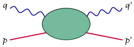
Figure 1: CS off the nucleon in general kinematics: $\gamma^{*}(q)N(p)\rightarrow\gamma^{*}(q^{\prime})N(p^{\prime})$.

However, as in any EFT framework, the convergence and the predictive power of $\chi$PT calculations are often of concern. After all, the expansion in energy and momenta is not as clear-cut as usual expansions in a small coupling constant. And, each new order brings more and more free parameters — the low-energy constants (LECs). This is why the cases where $\chi$PT provides true predictions are very valuable. One such case, considered here, is the process of Compton scattering (CS) off the nucleon, see Figure 1. It allows one to study the low-energy properties of the nucleon Bernard et al. (1991, 1992).

The nucleon is characterized by a number of different polarizabilities, the most important of which are the electric and magnetic dipole polarizabilities $\alpha_{E1}$ and $\beta_{M1}$. These quantities describe the size of the electric and magnetic dipole moments induced by an external electric $\vec{E}$ or magnetic $\vec{H}$ field:

$$\vec{d}_{\mathrm{ind.}} = 4\pi\alpha_{E1}\vec{E},$$ (1a)

$$\vec{\mu}_{\mathrm{ind.}} = 4\pi\beta_{M1}\vec{H}.$$ (1b)

In loosely bound systems, such as atoms and molecules, these polarizabilities are roughly given by the volume of the system. The nucleon is apparently a much more rigid object — its polarizabilities are orders of magnitude smaller than its volume ($\sim 1$ fm³). The most accurate evidence of that comes from the Baldin sum rule (sometimes referred to as the Baldin–Lapidus sum rule) Baldin (1960); Lapidus (1962). It is a very general relation based on the principles of causality, unitarity and crossing symmetry akin to the Kramers–Kronig relation (see, e.g., Ref. Pascalutsa (2018) for a pedagogical review). The Baldin sum rule expresses the sum of dipole polarizabilities in terms of an integral of the total photoabsorption cross section $\sigma_{T}$:

$$\alpha_{E1}+\beta_{M1}=\frac{1}{2\pi^{2}}\int_{\nu_{0}}^{\infty}\!\mathrm{d}\nu\,\frac{\sigma_{T}(\nu)}{\nu^{2}}.$$ (2)

Empirical evaluations Damashek and Gilman (1970); Schröder (1980); Babusci et al. (1998a); Levchuk and L’vov (2000); Olmos de León et al. (2001); Gryniuk et al. (2015), based on experimental cross sections of total photoabsorption on the nucleon, yield the most accurate information on proton and neutron dipole polarizabilities we presently have:

$$\alpha_{E1p}+\beta_{M1p} = 14.0(2)\times 10^{-4}\,\text{fm}^{3}\qquad\text{\cite[cite]{\@@bibref{Authors Phrase1YearPhrase2}{Gryniuk:2015eza}{\@@citephrase{(}}{\@@citephrase{)}}}},$$ (3a)

$$\alpha_{E1n}+\beta_{M1n} = 15.2(4)\times 10^{-4}\,\text{fm}^{3}\qquad\text{\cite[cite]{\@@bibref{Authors Phrase1YearPhrase2}{Levchuk:1999zy}{\@@citephrase{(}}{\@@citephrase{)}}}}.$$ (3b)

To disentangle $\alpha_{E1}$ and $\beta_{M1}$, one measures the angular distribution of low-energy CS. For example, the low-energy expansion of the unpolarized CS cross section is given by [to $\mathcal{O}(\nu^{2})$]:

$$\frac{\mathrm{d}\sigma}{\mathrm{d}\Omega_{L}}-\frac{\mathrm{d}\sigma^{\text{Born}}}{\mathrm{d}\Omega_{L}}=-\nu\nu^{\prime}\left(\frac{\nu^{\prime}}{\nu}\right)^{2}\frac{2\pi\alpha}{M_{N}}\left[\left(\alpha_{E1}+\beta_{M1}\right)(1+\cos\theta_{L})^{2}+\left(\alpha_{E1}-\beta_{M1}\right)(1-\cos\theta_{L})^{2}\right],$$ (4)

where $\theta_{L}$ is the scattering angle, $\mathrm{d}\Omega_{L}=2\pi\,\mathrm{d}\!\cos\theta_{L}$, and $\nu(\nu^{\prime})$ is the energy of the incoming (scattered) photon, all in the lab frame. Here, in addition to the sum of dipole polarizabilities appearing in forward kinematics, one can measure their difference. Another interesting observable is the beam asymmetry $\Sigma_{3}$ defined in Eq. (40), which also provides access to $\beta_{M1}$ independent of $\alpha_{E1}$ at $\mathcal{O}(\nu^{2})$, cf. Eq. (41).

In reality, the CS data are taken at finite energies (typically around 100 MeV), rather than at infinitesimal energies required for a strict validation of the above low-energy expansion. For a model-independent empirical extraction of polarizabilities from the RCS data it is, therefore, important to have a systematic theoretical framework such as $\chi$PT or a partial-wave analysis (PWA).

There are other interesting polarizabilities, called the spin polarizabilities. These are more difficult to visualise in a classical picture, but they certainly characterize the spin structure of the nucleon. $\chi$PT provides robust predictions for the different nucleon polarizabilities at leading and next-to-leading order. Given the accurate empirical knowledge of the nucleon polarizabilities from dispersive sum rules and CS experiments, they become an important benchmark for $\chi$PT in the single-baryon sector. But not just for $\chi$PT — the lattice QCD studies of nucleon polarizabilities are also closing in on the physical pion mass, see Figures 2 and 3.

It is worth mentioning that $\chi$PT can be used for calculating the proton-structure corrections to the muonic-hydrogen spectrum. These corrections are not only relevant in the context of the proton-radius puzzle Pohl et al. (2010); Antognini et al. (2013), but also for the planned measurements of the muonic-hydrogen ground-state hyperfine splitting Pohl et al. (2017); Bakalov et al. (2015); Kanda et al. (2018). The $\chi$PT is thusfar the only theoretical framework which can reliably compute the polarizability effects in CS observables and, at the same time, in atomic spectroscopy. In this way, a calculation which is validated on experimental data of CS and photoabsorption (through sum rules) can be used to predict the effects in muonic hydrogen Alarcón et al. (2014); Hagelstein and Pascalutsa (2016); Hagelstein (2017).

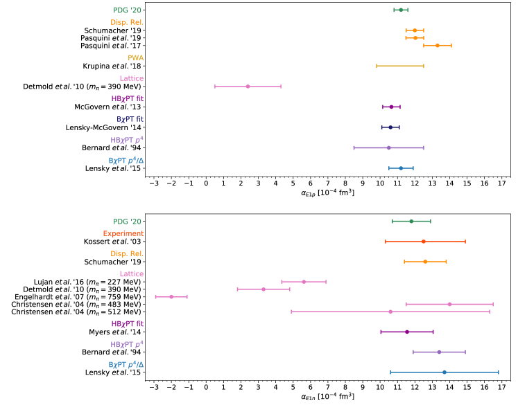
Figure 2: Summary for the electric dipole polarizability of the proton $\alpha_{E1p}$ (upper panel) and neutron $\alpha_{E1n}$ (lower panel). Theoretical predictions from chiral EFT and lattice QCD are compared with extractions based on CS data. Note that the lattice QCD calculations are done at unphysical pion masses. For the proton one observes a small tension between the dispersive approaches to CS and the B$\chi$PT results.

This mini-review is by no means comprehensive. A more proper review can be found in Ref. Hagelstein et al. (2016), whereas here I primarily provide an update on the nucleon polarizabilities. For the reader interested in the update only, I recommend to skip to Section 4 where a description of all summary plots is given. A recent theoretical discussion of nucleon polarizabilities in $\chi$PT and beyond can be found in Ref. Lensky and Pascalutsa (2019). Other commendable reviews include: Guichon and Vanderhaeghen (1998) or Fonvieille et al. (2020) (VCS and generalized polarizabilities), Drechsel et al. (2003) or Pasquini and Vanderhaeghen (2018) (dispersion relations for CS), Pascalutsa et al. (2007) ($\Delta(1232)$ resonance), Phillips (2009) (neutron polarizabilities), Griesshammer et al. (2012) ($\chi$EFT and RCS experiments), Holstein and Scherer (2014) (pion, kaon, nucleon polarizabilities), Geng (2013) (B$\chi$PT), Pascalutsa (2018) (dispersion relations), Deur et al. (2019) (nucleon spin structure). A textbook introduction to $\chi$PT can be found in Ref. Scherer and Schindler (2012).

The paper is organized as follows. In Sections 2 and 3, I briefly describe the $\chi$PT framework and the CS formalism. In Section 4, I summarize recent $\chi$PT results for the nucleon polarizabilities and compare to empirical and lattice QCD evaluations.

2 Baryon Chiral Perturbation Theory

The low-energy processes involving a nucleon, such as $\pi N$ scattering or CS off the nucleon, can be described by SU(2) baryon chiral perturbation theory (B$\chi$PT), which is the manifestly Lorentz-invariant variant of $\chi$PT in the single-baryon sector Gasser et al. (1988); Gegelia and Japaridze (1999); Fuchs et al. (2003). To introduce it, I will start in Section 2.1 with the basic EFT including only pions and nucleons. Then, in Section 2.2, I will discuss different ways (counting schemes) for incorporation of the lowest nucleon excitation — the $\Delta(1232)$ resonance — into the $\chi$PT framework. In Section 2.3, I will show how the LECs can be fit to experimental data and discuss the predictive power of $\chi$PT for CS. In Section 2.4, I introduce the heavy-baryon chiral perturbation theory (HB$\chi$PT) and point out how its predictions differ from B$\chi$PT for certain polarizabilities. For more details on B$\chi$PT for CS, I refer to the following series of calculations: RCS Lensky and Pascalutsa (2009, 2010); Lensky et al. (2015), VCS Lensky et al. (2017a) and forward VVCS Lensky et al. (2014); Alarcón et al. (2020a, b).

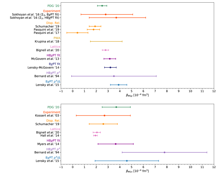
Figure 3: Summary for the magnetic dipole polarizability of the proton $\beta_{M1p}$ (upper panel) and neutron $\beta_{M1n}$ (lower panel). Theoretical predictions from chiral EFT and lattice QCD are compared with extractions based on CS data. Note that the lattice QCD results are extrapolated to the physical pion mass. For the proton one observes a small tension between the dispersive approaches to CS and the B$\chi$PT results.

2.1 B$\chi$PT with Pions and Nucleons

Consider the basic version of SU(2) B$\chi$PT including only pion and nucleon fields Gasser et al. (1988): scalar iso-vector $\pi^{a}(x)$ and spinor iso-doublet $\mathcal{N}(x)$. Expanding the EFT Lagrangian Gasser et al. (1988) to leading orders in pion derivatives, mass and fields, one finds (see, e.g., Ref. Ledwig et al. (2012)):

$$\mathcal{L}^{(1)}_{\mathcal{N}} = \overline{\mathcal{N}}\big{(}\not{D}-M_{N}\big{)}\mathcal{N}-\frac{g_{A}}{2f_{\pi}}\overline{\mathcal{N}}\,\tau^{a}\left(\not{D}^{ab}\pi^{b}\right)\gamma_{5}\,\mathcal{N},$$ (5a)

$$\mathcal{L}^{(2)}_{\pi} = \frac{1}{2}\Big{(}D_{\mu}^{ab}\pi^{b}\Big{)}\Big{(}D^{\mu}_{ac}\pi^{c}\Big{)}-\frac{1}{2}m_{\pi}^{2}\pi_{a}\pi^{a},$$ (5b)

with the covariant derivatives:

$$D_{\mu}^{ab}\pi^{b} = \delta^{ab}\partial_{\mu}\pi^{b}+ieQ_{\pi}^{ab}A_{\mu}\pi^{b},$$ (6a)

$$D_{\mu}\mathcal{N} = \partial_{\mu}\mathcal{N}+ieQ_{N}A_{\mu}\mathcal{N}+\frac{i}{4f_{\pi}^{2}}\,\varepsilon^{abc}\tau^{a}\pi^{b}(\partial_{\mu}\pi^{c}),$$ (6b)

the photon vector field $A_{\mu}(x)$, and the charges:

$$Q_{\pi}^{ab} = -i\varepsilon^{ab3},$$ (7a)

$$Q_{N} = \mbox{\small{$\frac{1}{2}\;$}}\!(1+\tau^{3}).$$ (7b)

Here, $\tau^{a}$ are the Pauli matrices, $\gamma_{5}=i\gamma^{0}\gamma^{1}\gamma^{2}\gamma^{3}$ are the Dirac matrices, $\varepsilon^{ijk}$ is the Levi-Cevita symbol, and all other parameters are introduced in Table 1.

The key ingredient for the development of $\chi$PT as a low-energy EFT of QCD was the observation that the pion couplings are proportional to their four-momenta Weinberg (1979); Gasser and Leutwyler (1984); Gasser et al. (1988). Therefore, at low momenta the couplings are weak and a perturbative expansion is possible. This chiral expansion is done in powers of pion momentum and mass, commonly denoted as $p$, over the scale of spontaneous chiral symmetry breaking, $\Lambda_{\chi\mathrm{SB}}\sim 4\pi f_{\pi}\approx 1$ GeV. Therefore, one expects that $\chi$PT provides a systematic description of the strong interaction at energies well below $1$ GeV. Considering only pion and nucleon fields, the chiral order $\mathcal{O}(p^{n})$ of a Feynman diagram with $L$ loops, $N_{\pi}$ ($N_{N}$) pion (nucleon) propagators, and $V_{k}$ vertices from $k$-th order Lagrangians [e.g., $k=1$: ${\gamma NN}$ interaction from Eq. (5a), $k=2$: ${\gamma\pi\pi}$ interaction from Eq. (5b)] is defined as Gasser et al. (1988):

$$n=4L-2N_{\pi}-N_{N}+\sum_{k}k\,V_{k}.$$ (8)

In the case of CS, the low-energy scale $p$ also includes the photon energy $\nu$ and virtuality $Q$, which therefore should be much smaller than $1$ GeV. However, the presence of bound states or low-lying resonances may lead to a breakdown of this perturbative expansion. For example, in $\pi\pi$ scattering the limiting scale of the perturbative expansion is set by the $\sigma(600)$ and $\rho(775)$ mesons Colangelo et al. (2001); Caprini et al. (2006). In the single-nucleon sector, the breakdown scale is set by the excitation energy of the first nucleon resonance, the $\Delta(1232)$ isobar. That is unless the $\Delta(1232)$ is included explicitly in the effective Lagrangian.

Table 1: LECs and other parameters and the orders at which they appear in the chiral expansion when employing the low-energy $\delta$-expansion counting scheme.

Order in
chiral expansion	$\chi$PT parameters		Values	Sources
	fine-structure constant	$\alpha=\nicefrac{{e^{2}}}{{4\pi}}$	$\simeq 1/137.04$
$\mathcal{O}(p^{2})$	nucleon mass	$M_{N}$	$938.27$ MeV
	nucleon axial charge	$g_{A}$	$1.27$	neutron decay $n\rightarrow p\,e^{-}\,\bar{\nu}_{e}$ Patrignani et al. (2016)
	pion decay constant	$f_{\pi}$	$92.21$ MeV	pion decay $\pi^{+}\rightarrow\mu^{+}\nu_{\mu}$ Patrignani et al. (2016)
$\mathcal{O}(p^{3})$	pion mass	$m_{\pi}$	$139.57$ MeV
				$P_{33}$ partial wave in $\pi N$ scattering
	$\mathcal{N}$-to-$\Delta$ axial coupling	$h_{A}$	$2.85$	and $\Delta(1232)$ decay width Pascalutsa et al. (2007); Pascalutsa and Vanderhaeghen (2005b, 2006b)
	$\Delta(1232)$ mass	$M_{\Delta}$	$1232$ MeV
	magnetic (M1) coupling	$g_{M}$	$2.97$
	electric (E2) coupling	$g_{E}$	$-1.0$
$\mathcal{O}(p^{4}/\varDelta)$	Coulomb (C2) coupling	$g_{\mathrm{C}}$	$-2.6$	pion electroproduction $e^{-}N\rightarrow e^{-}N\pi$ Pascalutsa and Vanderhaeghen (2006a)

2.2 Inclusion of the $\Delta(1232)$ and Power Counting

The $\Delta(1232)$ resonance as the lightest nucleon excitation has an excitation energy

$$\varDelta=M_{\Delta}-M_{N}\simeq 293\,\mathrm{MeV},$$ (9)

which is of the same order of magnitude as the pion mass. In the following, it will be included as an explicit degree of freedom: vector-spinor iso-quartet $\Delta_{\mu}(x)$. The relevant Lagrangians read Ledwig et al. (2012); Pascalutsa and Vanderhaeghen (2005a, 2006a):

$$\mathcal{L}^{(1)}_{\pi\Delta\mathcal{N}} = \frac{ih_{A}}{2f_{\pi}M_{\Delta}}\overline{\mathcal{N}}\,T^{a}\gamma^{\mu\nu\lambda}\left(D_{\mu}\Delta_{\nu}\right)\left(D_{\lambda}^{ab}\pi^{b}\right)+\text{h.c.},$$ (11a)

$$\mathcal{L}^{(2)\,\mathrm{non-minimal}}_{\gamma N\Delta} = \frac{3e}{2M_{N}(M_{N}+M_{\Delta})}\Bigg{[}\overline{\mathcal{N}}T_{3}\Big{\{}ig_{M}(\partial_{\mu}\Delta_{\nu})\tilde{F}^{\mu\nu}-g_{E}\gamma_{5}(\partial_{\mu}\Delta_{\nu})F^{\mu\nu}$$ (11b)

$$+i\frac{g_{\mathrm{C}}}{M_{\Delta}}\gamma_{5}\gamma^{\alpha}(\partial_{\alpha}\Delta_{\nu}-\partial_{\nu}\Delta_{\alpha})\partial_{\mu}F^{\mu\nu}\Big{\}}+\text{h.c.}\Bigg{]},$$

with the covariant derivative:

$$D_{\mu}\Delta_{\nu}=\partial_{\mu}\Delta_{\nu}+ieQ_{\Delta}A_{\mu}\Delta_{\nu}+\frac{i}{2f_{\pi}^{2}}\,\varepsilon^{abc}\,\mathscr{T}^{a}\pi^{b}(\partial_{\mu}\pi^{c}),$$ (12)

and the charge:

$$Q_{\Delta}=\mbox{\small{$\frac{1}{2}\;$}}\!(1+3\mathscr{T}^{3}).$$ (13)

Here, h.c. stands for the hermitian conjugate, $\gamma^{\mu\nu}=-\frac{i}{2}\epsilon^{\mu\nu\alpha\beta}\gamma_{\alpha}\gamma_{\beta}\gamma^{5}$ and $\gamma^{\mu\nu\alpha}=-i\epsilon^{\mu\nu\alpha\beta}\gamma_{\beta}\gamma^{5}$ are Dirac matrices with $\epsilon_{0123}=1$, $F^{\mu\nu}=\partial^{\mu}A^{\nu}-\partial^{\nu}A^{\mu}$ is the electromagnetic field strength tensor, $\tilde{F}^{\mu\nu}=\epsilon^{\mu\nu\rho\lambda}\partial_{\rho}A_{\lambda}$ is its dual, and $T^{a}$ ($\mathscr{T}^{a}$) are the isospin $1/2$ ($3/2$) to $3/2$ transition matrices. The latter commute with the Dirac matrices. The superscripts of the Lagrangians in Eqs. (5) and (11) denote their order as reflected by the number of comprised small quantities: pion mass, momentum and factors of $e$. Inclusion of the $\Delta(1232)$ introduces the excitation energy $\varDelta$ as another small scale, which has to be considered when defining a power-counting for the perturbative $\chi$PT expansion.

There are two prominent counting schemes for $\chi$PT with explicit inclusion of the $\Delta(1232)$. For simplicity, they both deduce a single expansion parameter from the two involved small mass scales: $\epsilon=m_{\pi}/\Lambda_{\chi\mathrm{SB}}$ and $\delta=\varDelta/\Lambda_{\chi\mathrm{SB}}$. In the $\epsilon$-expansion (small-scale expansion) it is assumed that $\epsilon\sim\delta$ Hemmert et al. (1997a), while in the $\delta$-expansion one assumes $\epsilon\sim\delta^{2}$ with $\epsilon\ll\delta$ Pascalutsa and Phillips (2003). In this way, the $\delta$-expansion defines a hierarchy between the two mass scales. Consequently, it defines two regimes where the $\Delta(1232)$ contributions need to be counted differently:

• low-energy region: $p\sim m_{\pi}$;

• resonance region: $p\sim\varDelta$.

This makes sense since the $\Delta(1232)$ is expected to be suppressed at low energies and dominating in the resonance region. The chiral order $\mathcal{O}(p^{n_{\delta}})$ of a Feynman diagram with $N_{\text{1$\Delta$R}}$ ($N_{\text{1$\Delta$I}}$) one-$\Delta$-reducible (one-$\Delta$-irreducible) propagators is in the $\delta$-expansion defined as:

$$n_{\delta}=\begin{cases}n-\nicefrac{{1}}{{2}}\,N_{\Delta}\,,&p\sim m_{\pi},\\ n-3N_{\text{1$\Delta$R}}-N_{\text{1$\Delta$I}}\,,&p\sim\Delta,\end{cases}$$ (14)

where

$$N_{\Delta}=N_{\text{1$\Delta$R}}+N_{\text{1$\Delta$I}}.$$ (15)

An extensive review on the electromagnetic excitation of the $\Delta$(1232) resonance with more details on the formulation of the extended $\chi$PT framework and the chiral expansion in the resonance region can be found in Ref. Pascalutsa et al. (2007). As we will see in Section 4, B$\chi$PT calculations based on the $\epsilon$ Bernard et al. (2013) and the $\delta$ Lensky et al. (2014); Alarcón et al. (2020b) counting schemes give significantly different predictions for the longitudinal-transverse polarizability of the proton shown in Figures 4 (upper panel) and 5.

2.3 Low-Energy Constants and Predictive Orders

At any given order in the chiral expansion, the divergencies of the EFT are absorbed by renormalization of a finite number of LECs. To match $\chi$PT to QCD as the fundamental theory of the strong interaction, the renormalized LECs need to be fitted to experimental or lattice data. Thereby, it is important that the LECs are constrained to be of natural size. Take for instance the fifth-order forward spin polarizability (in units of $10^{-4}$ fm⁶) Alarcón et al. (2020b):

$$\bar{\gamma}_{0p}=1.12(30)\approx 2.08\,\mbox{($\pi$N loop)}-0.96\,\mbox{($\Delta$ exchange)}-0.01\,\mbox{($\pi\Delta$ loop)},$$ (16a)

$$\bar{\gamma}_{0n}=1.95(30)\approx 2.92\,\mbox{($\pi$N loop)}-0.96\,\mbox{($\Delta$ exchange)}-0.01\,\mbox{($\pi\Delta$ loop)},$$ (16b)

also shown in Figure 6. The next-to-leading-order effect of the $\Delta(1232)$ is two to three times smaller than the leading-order effect of the pion cloud. This is consistent with estimates from power counting, according to which each subleading order is expected to be suppressed with respect to the previous one by a factor of $\sim\varDelta/M_{N}\sim 1/3$. Therefore, implementing this naturalness allows to estimate the uncertainty due to neglect of higher-order effects.

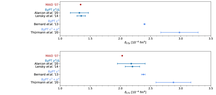
Figure 4: Summary for the longitudinal-transverse polarizability of the proton $\delta_{LTp}$ (upper panel) and neutron $\delta_{LTn}$ (lower panel). Theoretical predictions from chiral EFT are compared to the MAID unitary isobar model.

The LECs entering a next-to-next-to-leading-order B$\chi$PT calculation of low-energy CS in the $\delta$-expansion are $f_{\pi}$, $g_{A}$, $h_{A}$, $g_{M}$, $g_{E}$ and $g_{C}$. They are listed in Table 1 together with the experiments used to constrain their values. As one can see, B$\chi$PT has “predictive power” for low-energy CS up to and including $\mathcal{O}(p^{4}/\varDelta)$ because all relevant LECs are matched to processes other than CS. This makes $\chi$PT the perfect tool to study the low-energy structure of the nucleon as encoded in CS and the associated polarizabilities. Starting from $\mathcal{O}(p^{4})$, LECs need to be fitted to the CS process as well, for instance through the Baldin sum rule, as done in Refs. McGovern et al. (2013); Griesshammer et al. (2012); Lensky and McGovern (2014); Myers et al. (2014, 2015); Griesshammer et al. (2016); Alarcón et al. (2020a).

2.4 Heavy-Baryon Expansion

The theory of HB$\chi$PT was first introduced in Ref. Jenkins and Manohar (1991), and later applied to CS and polarizabilities Butler and Savage (1992), including also the effect of the $\Delta(1232)$ Bernard et al. (1995); Hemmert et al. (1997b); Hildebrandt et al. (2004); Griesshammer et al. (2012); Kao et al. (2003, 2004); Nevado and Pineda (2008). The results of HB$\chi$PT can be recovered from the B$\chi$PT results by expanding in powers of the inverse nucleon mass. HB$\chi$PT calculations tend to fail in describing the $Q^{2}$ evolution of the generalized nucleon polarizabilities Alarcón et al. (2020b, a). Also for the polarizabilities at the real-photon point ($Q^{2}=0$) the heavy-baryon expansion can give significantly different predictions. Consider for instance the nucleon dipole polarizabilities. The B$\chi$PT prediction (in units of $10^{-4}\,$fm³) Lensky et al. (2015):

$$\alpha_{E1p} = 6.9\,\mbox{($\pi$N loop)}-0.1\,\mbox{($\Delta$ exchange)}+4.4\,\mbox{($\pi\Delta$ loop)}=11.2\pm 0.7,$$ (17a)

$$\beta_{M1p} = -1.8\,\mbox{($\pi$N loop)}+7.1\,\mbox{($\Delta$ exchange)}-1.4\,\mbox{($\pi\Delta$ loop)}=3.9\pm 0.7,$$ (17b)

is in good agreement with empirical evaluations, see Figures 2 and 3. In HB$\chi$PT, however, the $\Delta(1232)$ contributions to the nucleon polarizabilities turn out to be large Hemmert et al. (1997b) and need to be canceled by promoting the higher-order [$\mathcal{O}(p^{4})$] counterterms $\delta\alpha$ and $\delta\beta$ (in units of $10^{-4}\,$fm³) Hildebrandt et al. (2004):

$$\alpha_{E1p}(\mbox{HB}) = 11.87\,\mbox{($\pi$N loop)}+0\,\mbox{($\Delta$ exch.)}+5.09\,\mbox{($\pi\Delta$ loop)}-(5.92\pm 1.36)\,\mbox{($\delta\alpha$)}$$ (18a)

$$= 11.04\pm 1.36\,,$$

$$\beta_{M1p}(\mbox{HB}) = 1.25\,\mbox{($\pi$N loop)}+(11.33\pm 0.70)\,\mbox{($\Delta$ exch.)}+0.86\,\mbox{($\pi\Delta$ loop)}$$ (18b)

$$-(10.68\pm 1.17)\,\mbox{($\delta\beta$)}\qquad$$

$$= 2.76\mp 1.36,$$

at the expense of violating the naturalness requirement, see also Ref. Griesshammer et al. (2012). This can be seen from the dimensionless LECs associated to $\delta\alpha$ and $\delta\beta$, $g_{117}=18.82\pm 0.79$ and $g_{118}=-6.05\mp 0.66$ Hildebrandt et al. (2004), that should be of $\mathcal{O}(1)$ to be consistent with estimates from power counting. This problem is discussed at length in Refs. Lensky and Pascalutsa (2010); Hall and Pascalutsa (2012).

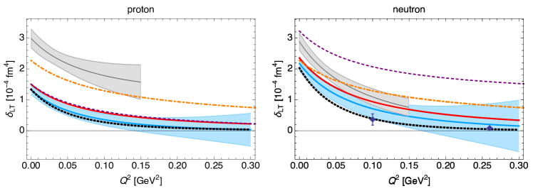
Figure 5: Longitudinal-transverse spin polarizability, Eq. (39), for the proton (left) and neutron (right) as function of $Q^{2}$. The black dotted line is the MAID model Drechsel et al. (2001, 1999); note that for the proton we use the updated estimate from Ref. Drechsel et al. (2003) obtained using the $\pi,\eta,\pi\pi$ channels. The red line shows the leading-order B$\chi$PT result. The blue band is the $\mathcal{O}(p^{4}/\Delta)$ B$\chi$PT result from Ref. Alarcón et al. (2020b). The gray band is the $\mathcal{O}(\epsilon^{3}+p^{4})$ B$\chi$PT result from Ref. Thürmann et al. (2020). The orange dot-dashed and purple short-dashed lines are the $\mathcal{O}(p^{3})$ and $\mathcal{O}(p^{4})$ HB results from Ref. Kao et al. (2003). The experimental points for the neutron are from Ref. Amarian et al. (2004) (blue diamonds).

3 Compton Scattering Formalism

The CS process, shown in Figure 1, gives the most direct access to the nucleon polarizabilities. Of interest are the following kinematic regimes, described by the four-momenta of incoming (outgoing) photons $q(q^{\prime})$ and nucleons $p(p^{\prime})$:

• Real Compton scattering (RCS): $q^{2}=q^{\prime\,2}=0$;

• Virtual Compton scattering (VCS): $q^{2}=-Q^{2}<0$ and $q^{\prime\,2}=0$;

• Forward doubly-virtual Compton scattering (VVCS): $q=q^{\prime}$ (thus $p=p^{\prime}$) and $q^{2}=-Q^{2}<0$.

In general kinematics ($p^{2}=p^{\prime\,2}=M_{N}^{2}$, $q^{2}\neq q^{\prime\,2}$), the CS amplitude can be described by $18$ independent tensor structures. For VCS one needs $12$ independent tensor structures; for RCS one needs $6$ independent tensor structures Hearn and Leader (1962); Babusci et al. (1998b). In the forward limit, this reduces to $4$ independent tensor structures for virtual photons and $2$ independent tensor structures for real photons.

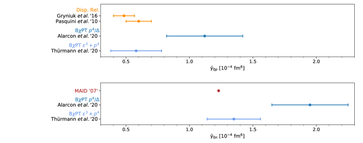
Figure 6: Summary for the fifth-order forward spin polarizability of the proton $\bar{\gamma}_{0p}$ (upper panel) and neutron $\bar{\gamma}_{0n}$ (lower panel). Theoretical predictions from chiral EFT are compared to empirical evaluations of the fifth-order forward spin polarizability sum rule (37) at the real-photon point and the MAID unitary isobar model.

Splitting into spin-independent (symmetric) and spin-dependent (antisymmetric) parts, the forward VVCS decomposes into four scalar amplitudes $T_{i}(\nu,Q^{2})$ and $S_{i}(\nu,Q^{2})$:

$$T^{\mu\nu}(q,p)=\left[T^{\mu\nu}_{S}+T^{\mu\nu}_{A}\right](q,p),$$ (19a)

with

$$T^{\mu\nu}_{S}(q,p) = -g^{\mu\nu}\,T_{1}(\nu,Q^{2})+\frac{p^{\mu}p^{\nu}}{M_{N}^{2}}\,T_{2}(\nu,Q^{2}),$$ (19b)

$$T^{\mu\nu}_{A}(q,p) = -\frac{1}{M_{N}}\gamma^{\mu\nu\alpha}q_{\alpha}\,S_{1}(\nu,Q^{2})+\frac{Q^{2}}{M_{N}^{2}}\gamma^{\mu\nu}S_{2}(\nu,Q^{2}),$$ (19c)

with $\nu$ the photon lab-frame energy, $Q^{2}$ the photon virtuality, and terms which vanish upon contraction with the photon polarization vectors omitted. For real photons, the following two scalar amplitudes survive:

$$f(\nu)=\frac{1}{4\pi}T_{1}(\nu,0),\qquad g(\nu)=\frac{\nu}{4\pi M_{N}}S_{1}(\nu,0).$$ (20)

Constraints relating the different kinematic regimes (RCS, VCS and forward VVCS) are discussed in Refs. Lensky et al. (2018) and Pascalutsa and Vanderhaeghen (2015); Lensky et al. (2017b) for the unpolarized and polarized CS, respectively. Here, the focus is on RCS and forward VVCS.

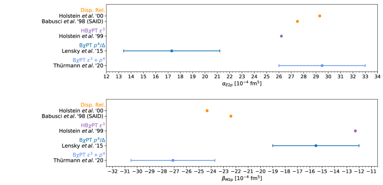
Figure 7: Summary for the quadrupole polarizabilities $\alpha_{E2p}$ and $\beta_{M2p}$ of the proton. Theoretical predictions from chiral EFT are compared with extractions based on CS data.

The off-forward RCS is conveniently described by the covariant decomposition Pascalutsa and Phillips (2003):

$$\bar{u}^{\,\prime}(\varepsilon^{\prime}\cdot T\cdot\varepsilon)u=4\pi\alpha\,\hat{\mathscr{A}}^{T}(s,t)\,\bar{u}^{\,\prime}\hat{\mathscr{O}}^{\mu\nu}u\,\mathcal{E}_{\mu}^{\prime}\mathcal{E}_{\nu},$$ (21a)

with the overcomplete set of $$8$$ tensors:

$$\hat{\mathscr{A}}(s,t)=\big{\{}\mathscr{A}_{1},\,\cdots,\,\mathscr{A}_{8}\big{\}}(s,t),$$ (21b)

$$\hat{\mathscr{O}}^{\mu\nu}=\big{\{}-g^{\mu\nu},\;q^{\mu}q^{\prime\,\nu},\;-\gamma^{\mu\nu},\;g^{\mu\nu}(q^{\prime}\cdot\gamma\cdot q),\;q^{\mu}q^{\prime}_{\alpha}\gamma^{\alpha\nu}-\gamma^{\alpha\mu}q_{\alpha}q^{\prime\nu},\;q^{\mu}q_{\alpha}\gamma^{\alpha\nu}-\gamma^{\alpha\mu}q^{\prime}_{\alpha}q^{\prime\nu},$$

$$\qquad\qquad q^{\mu}q^{\prime\,\nu}(q^{\prime}\cdot\gamma\cdot q),\;-i\gamma_{5}\epsilon^{\mu\nu\alpha\beta}q^{\prime}_{\alpha}q_{\beta}\big{\}},$$ (21c)

$$\mathcal{E}_{\mu}=\varepsilon_{\mu}-\frac{P\cdot\varepsilon}{P\cdot q}\,q_{\mu},\quad\mathcal{E}_{\mu}^{\prime}=\varepsilon_{\mu}^{\prime}-\frac{P\cdot\varepsilon^{\prime}}{P\cdot q}\,q_{\mu}^{\prime},\quad P_{\mu}=\mbox{\small{$\frac{1}{2}\;$}}(p+p^{\prime})_{\mu},\quad P\cdot q=P\cdot q^{\prime},$$ (21d)

and the incoming (outgoing) photon polarization vector $\varepsilon^{(\prime)}$ and Dirac spinor $u^{(\prime)}$. Alternatively, one can choose the non-covariant decomposition with the minimal set of $6$ tensors:

$$\bar{u}^{\,\prime}(\varepsilon^{\prime}\cdot T\cdot\varepsilon)u=8\pi\alpha M_{N}\,\hat{A}^{T}(s,t)\,\chi^{\,\prime}\varepsilon_{i}^{\prime}\,\hat{O}_{ij}\,\varepsilon_{j}\,\chi,$$ (22a)

with the incoming (outgoing) Pauli spinor $$\chi^{(\prime)}$$ and the scalar complex amplitudes Hemmert et al. (1998):

$$\hat{A}(s,t)=\big{\{}A_{1},\,\cdots,\,A_{6}\big{\}}(s,t),$$ (22b)

$$\hat{O}_{ij}=\big{\{}\delta_{ij},\,n_{i}n_{j}^{\prime},\,i\epsilon_{ijk}\sigma_{k},\,\delta_{ij}i\epsilon_{klm}\sigma_{k}n_{l}^{\prime}n_{m},\,i\epsilon_{klm}\sigma_{k}(\delta_{il}n_{m}n_{j}^{\prime}-\delta_{jl}n_{i}n_{m}^{\prime}),$$

$$\qquad\qquad i\epsilon_{klm}\sigma_{k}(\delta_{il}n_{m}^{\prime}n_{j}^{\prime}-\delta_{jl}n_{i}n_{m})\big{\}},\qquad\qquad$$ (22c)

where $\vec{n}^{(\prime)}$ is the direction of the incoming (outgoing) photon, $\sigma_{k}$ are the Pauli matrices and $\delta_{ij}$ is the Kronecker delta. The scalar amplitudes $\mathscr{A}_{1,\dots,8}$ are related to the scalar amplitudes $A_{1,\dots,6}$ in the following way McGovern et al. (2013):

$$A_{1} = \frac{\epsilon_{B}}{M_{N}}\mathscr{A}_{1}+\frac{\omega_{B}t}{2M_{N}}\mathscr{A}_{4},$$ (23a)

$$A_{2} = \frac{\epsilon_{B}\omega_{B}^{2}}{M_{N}}\mathscr{A}_{2}+\frac{\omega_{B}^{3}}{M_{N}}\left(\mathscr{A}_{5}+\mathscr{A}_{6}-\mbox{\small{$\frac{1}{2}\;$}}t\mathscr{A}_{7}\right),$$ (23b)

$$A_{3} = \frac{\epsilon_{B}}{M_{N}}\mathscr{A}_{3}-\frac{M_{N}^{2}\eta\,t}{4M_{N}^{2}-t}\left(\frac{\mathscr{A}_{5}+\mathscr{A}_{6}}{2M_{N}(\epsilon_{B}+M_{N})}-\mathscr{A}_{7}\right)-\frac{\omega_{B}t}{2M_{N}}\mathscr{A}_{8},$$ (23c)

$$A_{4} = \omega_{B}^{2}\mathscr{A}_{4},$$ (23d)

$$A_{5} = \omega_{B}^{2}\mathscr{A}_{5}+\frac{\omega_{B}^{2}}{2M_{N}(\epsilon_{B}+M_{N})}\Big{[}\mbox{\small{$\frac{1}{2}\;$}}\mathscr{A}_{3}+\frac{M_{N}^{2}\eta}{4M_{N}^{2}-t}\left(\mathscr{A}_{5}+\mathscr{A}_{6}\right)\Big{]}-\omega_{B}^{2}(\omega_{B}^{2}+\mbox{\small{$\frac{1}{2}\;$}}t)\mathscr{A}_{7}+\frac{\omega_{B}^{3}}{2M_{N}}\mathscr{A}_{8},\qquad$$ (23e)

$$A_{6} = \omega_{B}^{2}\mathscr{A}_{6}-\frac{\omega_{B}^{2}}{2M_{N}(\epsilon_{B}+M_{N})}\Big{[}\mbox{\small{$\frac{1}{2}\;$}}\mathscr{A}_{3}+\frac{M_{N}^{2}\eta}{4M_{N}^{2}-t}\left(\mathscr{A}_{5}+\mathscr{A}_{6}\right)\Big{]}+\omega_{B}^{4}\mathscr{A}_{7}-\frac{\omega_{B}^{3}}{2M_{N}}\mathscr{A}_{8},$$ (23f)

where

$$\omega_{B} = \frac{s-u}{2\sqrt{4M_{N}^{2}-t}},$$ (24a)

$$\epsilon_{B} = \frac{1}{2}\sqrt{4M_{N}^{2}-t}.$$ (24b)

are the nucleon and photon energies in the Breit frame ($\vec{p}^{\prime}=-\vec{p}\,$),

$$\eta=\frac{M_{N}^{4}-su}{M_{N}^{2}},$$ (25)

and $s$, $t$, $u$ are the usual Mandelstam variables.

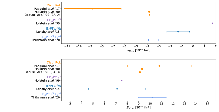
Figure 8: Summary for the dispersive polarizabilities of the proton, $\alpha_{E1\nu p}$ and $\beta_{M1\nu p}$. Theoretical predictions from chiral EFT are compared with extractions based on CS data. Note that Pasquini et al. ’17 Pasquini et al. (2018) presented the first extraction of the dispersive polarizabilities from proton RCS data below pion-production threshold.

According to the low-energy theorem of Low Low (1954), Gell-Mann and Goldberger Gell-Mann and Goldberger (1954), the leading terms in a low-energy expansion of the RCS amplitudes are determined by charge, mass and anomalous magnetic moment of the nucleon. At higher orders in the low-energy expansion various polarizabilities emerge. The low-energy expansion of the non-Born RCS amplitudes (denoted by an overline, e.g., $\bar{A}_{1,\dots,6}$) reads as:

$$\alpha\bar{A}_{1}(\omega_{B},t) = \omega_{B}^{2}\big{[}\alpha_{E1}+\beta_{M1}+\omega_{B}^{2}\,(\alpha_{E1\nu}+\beta_{M1\nu})\,\big{]}+\mbox{\small{$\frac{1}{2}\;$}}t\big{(}\beta_{M1}+\omega_{B}^{2}\beta_{M1\nu}\,\big{)}$$ (26a)

$$+\;\omega_{B}^{4}\mbox{$\frac{1}{12}$}(\alpha_{E2}+\beta_{M2})+\mbox{\small{$\frac{1}{2}\;$}}t(4\omega_{B}^{2}+t)\mbox{$\frac{1}{12}$}\beta_{M2}+\mathcal{O}(\omega_{B}^{6}),$$

$$\alpha\bar{A}_{2}(\omega_{B},t) = -\omega_{B}^{2}\big{(}\beta_{M1}+\omega_{B}^{2}\beta_{M1\nu}\big{)}+\omega_{B}^{4}\mbox{$\frac{1}{12}$}(\alpha_{E2}-\beta_{M2})-t\omega_{B}^{2}\mbox{$\frac{1}{12}$}\beta_{M2}+\mathcal{O}(\omega_{B}^{6}),$$ (26b)

$$\alpha\bar{A}_{3}(\omega_{B},t) = -\omega_{B}^{3}\,\big{[}\gamma_{E1E1}+\gamma_{E1M2}+z\,(\gamma_{M1E2}+\gamma_{M1M1})\big{]}+\mathcal{O}(\omega_{B}^{5}),$$ (26c)

$$\alpha\bar{A}_{4}(\omega_{B},t) = \omega_{B}^{3}\,(\gamma_{M1E2}-\gamma_{M1M1})+\mathcal{O}(\omega_{B}^{5}),$$ (26d)

$$\alpha\bar{A}_{5}(\omega_{B},t) = \omega_{B}^{3}\,\gamma_{M1M1}+\mathcal{O}(\omega_{B}^{5}),$$ (26e)

$$\alpha\bar{A}_{6}(\omega_{B},t) = \omega_{B}^{3}\,\gamma_{E1M2}+\mathcal{O}(\omega_{B}^{5}),$$ (26f)

with $z=\cos\theta_{B}=1+t/2\omega_{B}^{2}$ and $\theta_{B}$ the scattering angle in the Breit frame. The coefficients are given in terms of static nucleon polarizabilities: electric dipole ($\alpha_{E1}$), magnetic dipole ($\beta_{M1}$), quadrupole ($\alpha_{E2}$, $\beta_{M2}$), dispersive ($\alpha_{E1\nu}$, $\beta_{M1\nu}$), and lowest-order spin polarizabilities ($\gamma_{E1E1}$, $\gamma_{M1M1}$, $\gamma_{E1M2}$ and $\gamma_{M1E2}$), see Figures 2, 3, 7, 8 and 9, respectively. The latter combine into the forward (see Figure 10) and backward spin polarizabilities:

$$\gamma_{0} = -\gamma_{E1E1}-\gamma_{M1M1}-\gamma_{E1M2}-\gamma_{M1E2},$$ (27a)

$$\gamma_{\pi} = -\gamma_{E1E1}+\gamma_{M1M1}-\gamma_{E1M2}+\gamma_{M1E2}.$$ (27b)

Studying the forward RCS and VVCS is of advantage because of their accessibility through sum rules. Based on the general principles of causality, unitarity and crossing symmetry, the forward VVCS amplitudes can be expressed in terms of the nucleon structure functions by means of dispersion relations and the optical theorem Drechsel et al. (2003):

$$T_{1}(\nu,Q^{2}) = T_{1}(0,Q^{2})+\frac{32\pi\alpha M_{N}\nu^{2}}{Q^{4}}\int_{0}^{1}\!\mathrm{d}x\,\frac{x\,f_{1}(x,Q^{2})}{1-x^{2}(\nu/\nu_{\mathrm{el}})^{2}-i0^{+}}$$

$$= T_{1}(0,Q^{2})+\frac{2\nu^{2}}{\pi}\int_{\nu_{\mathrm{el}}}^{\infty}\!\frac{\mathrm{d}\nu^{\prime}}{\nu^{\prime}}\,\frac{\sqrt{\nu^{\prime\,2}+Q^{2}}\,\sigma_{T}(\nu^{\prime},Q^{2})}{\nu^{\prime\,2}-\nu^{2}-i0^{+}}\,,$$

$$T_{2}(\nu,Q^{2}) = \frac{16\pi\alpha M_{N}}{Q^{2}}\int_{0}^{1}\!\mathrm{d}x\,\frac{f_{2}(x,Q^{2})}{1-x^{2}(\nu/\nu_{\mathrm{el}})^{2}-i0^{+}}$$

$$= \frac{2Q^{2}}{\pi}\int_{\nu_{\mathrm{el}}}^{\infty}\!\mathrm{d}\nu^{\prime}\,\frac{\nu^{\prime}\,[\sigma_{T}+\sigma_{L}](\nu^{\prime},Q^{2})}{\sqrt{\nu^{\prime\,2}+Q^{2}}(\nu^{\prime\,2}-\nu^{2}-i0^{+})},$$

$$S_{1}(\nu,Q^{2}) = \frac{16\pi\alpha M_{N}}{Q^{2}}\int_{0}^{1}\!\mathrm{d}x\,\frac{g_{1}(x,Q^{2})}{1-x^{2}(\nu/\nu_{\mathrm{el}})^{2}-i0^{+}}$$

$$= \frac{2M_{N}}{\pi}\int_{\nu_{\mathrm{el}}}^{\infty}\!\mathrm{d}\nu^{\prime}\,\frac{\nu^{\prime\,2}\big{[}\frac{Q}{\nu^{\prime}}\sigma_{LT}+\sigma_{TT}\big{]}(\nu^{\prime},Q^{2})}{\sqrt{\nu^{\prime\,2}+Q^{2}}(\nu^{\prime\,2}-\nu^{2}-i0^{+})},$$

$$\nu S_{2}(\nu,Q^{2}) = \frac{16\pi\alpha M_{N}^{2}}{Q^{2}}\int_{0}^{1}\!\mathrm{d}x\,\frac{g_{2}(x,Q^{2})}{1-x^{2}(\nu/\nu_{\mathrm{el}})^{2}-i0^{+}}$$

$$= \frac{2M_{N}^{2}}{\pi}\int_{\nu_{\mathrm{el}}}^{\infty}\!\mathrm{d}\nu^{\prime}\,\frac{\nu^{\prime\,2}\big{[}\frac{\nu^{\prime}}{Q}\sigma_{LT}-\sigma_{TT}\big{]}(\nu^{\prime},Q^{2})}{\sqrt{\nu^{\prime\,2}+Q^{2}}(\nu^{\prime\,2}-\nu^{2}-i0^{+})},$$

with $\nu_{\mathrm{el}}=Q^{2}/2M_{N}$ the elastic threshold. Note that the structure functions $f_{1}$, $f_{2}$, $g_{1}$ and $g_{2}$ are functions of the Bjorken variable $x=\nu_{\mathrm{el}}/\nu$ and the photon virtuality $Q^{2}$. They are related to the photoabsorption cross sections $\sigma_{T}$, $\sigma_{L}$, $\sigma_{TT}$ and $\sigma_{LT}$ measured in electroproduction, defined here with the photon flux factor $K(\nu,Q^{2})=\sqrt{\nu^{2}+Q^{2}}$ Gilman (1968).

Performing low-energy expansions of the relativistic CS amplitudes Drechsel et al. (1998, 2003); Pascalutsa and Vanderhaeghen (2015) and combining these with dispersion relations and the optical theorem leads to various sum rules for the polarizabilities. A famous sum-rule example is the Baldin sum rule Baldin (1960), allowing for a precise data-driven evaluation of the sum of electric and magnetic dipole polarizabilities, cf. Eqs. (2) and (3). It follows from the $\nu^{2}$ term in the low-energy expansion of the RCS amplitude $f(\nu)$:

$$f(\nu)=-\,\frac{Z^{2}\alpha}{M_{N}}+\left[\alpha_{E1}+\beta_{M1}\right]\,\nu^{2}+\left[\alpha_{E1\nu}+\beta_{M1\nu}+\nicefrac{{1}}{{12}}\,(\alpha_{E2}+\beta_{M2})\right]\,\nu^{4}+\mathcal{O}(\nu^{6}).$$ (29)

The extension of the Baldin sum rule to finite momentum-transfers Drechsel et al. (2003),

$$\left[\alpha_{E1}+\beta_{M1}\right](Q^{2})=\frac{1}{2\pi^{2}}\int_{\nu_{0}}^{\infty}\!\mathrm{d}\nu\,\sqrt{1+\frac{Q^{2}}{\nu^{2}}}\,\frac{\sigma_{T}(\nu,Q^{2})}{\nu^{2}},$$ (30)

defines the $Q^{2}$ dependent sum of generalized dipole polarizabilities. Be aware that while the definitions of the polarizabilities in the real-photon limit are unambiguous, the generalized polarizabilities defined in VCS and forward VVCS can differ. As an example, one can consider the magnetic dipole polarizability $\beta_{M1}(Q^{2})$, which for VCS is defined in Eq. (B2b) of Ref. Lensky et al. (2018), and for forward VVCS could be defined either by generalizing the non-Born part of the subtraction function

$$\frac{\overline{T}_{1}(0,Q^{2})}{4\pi}=\beta_{M1}Q^{2}+\mathcal{O}(Q^{4}),$$ (31)

but is usually understood as part of the generalized Baldin sum rule (30). A recent measurement of the generalized $\alpha_{E1}(Q^{2})$ and $\beta_{M1}(Q^{2})$ polarizabilities from VCS by the A1 Collaboration can be found in Ref. Beričič et al. (2019).

The generalized fourth-order Baldin sum rule is defined as:

$$M_{1}^{(4)}(Q^{2})=\frac{1}{2\pi^{2}}\,\int_{\nu_{0}}^{\infty}\,\mathrm{d}\nu\,\sqrt{1+\frac{Q^{2}}{\nu^{2}}}\,\frac{\sigma_{T}(\nu,Q^{2})}{\nu^{4}}.$$ (32)

It differs from the generalized Baldin sum rule (30) by the energy weighting of the total photoabsorption cross section $\sigma_{T}$ in the sum rule integral. In the real-photon limit, it is related to a linear combination of the dispersive and quadrupole polarizabilities given by the $\nu^{4}$ term in Eq. (29) Guiasu and Radescu (1979); Holstein et al. (2000):

$$M_{1}^{(4)}(0)=\alpha_{E1\nu}+\beta_{M1\nu}+\frac{1}{12}(\alpha_{E2}+\beta_{M2}),$$ (33)

see Figure 11.

Similarly, the low-energy expansion of the RCS amplitude $g(\nu)$:

$$g(\nu)=-\frac{\alpha\kappa_{N}^{2}}{2M_{N}^{2}}\,\nu+\gamma_{0}\,\nu^{3}+\bar{\gamma}_{0}\,\nu^{5}+\mathcal{O}(\nu^{6}),$$ (34)

allows to express the anomalous magnetic moment of the nucleon ($\kappa_{p}\sim 1.79,\kappa_{n}\sim-1.91$) and the forward spin polarizabilities as sum rule integrals over the helicity-difference photoabsorption cross section $\sigma_{TT}$, cf. Eq. (28). The Gerasimov–Drell–Hearn sum rule Gerasimov (1966); Drell and Hearn (1966):

$$-\frac{\alpha}{2M_{N}^{2}\kappa_{N}^{2}}=\frac{1}{2\pi^{2}}\int_{\nu_{0}}^{\infty}\!\mathrm{d}\nu\,\frac{\sigma_{TT}(\nu)}{\nu},$$ (35)

has been experimentally verified for the nucleon by MAMI (Mainz) and ELSA (Bonn) Ahrens et al. (2001); Helbing (2002). The same cross section input can be used to evaluate the forward spin polarizabilities at the real-photon point, cf. Figures 10 and 6. Considering the extension to finite momentum-transfers, the generalized forward spin polarizability reads Drechsel et al. (2003):

$$\gamma_{0}(Q^{2})=\frac{1}{2\pi^{2}}\int_{\nu_{0}}^{\infty}\!\mathrm{d}\nu\,\sqrt{1+\frac{Q^{2}}{\nu^{2}}}\,\frac{\sigma_{TT}(\nu,Q^{2})}{\nu^{3}},$$ (36)

while the fifth-order generalized forward spin polarizability sum rule is given by:

$$\bar{\gamma}_{0}(Q^{2})=\frac{1}{2\pi^{2}}\int_{\nu_{0}}^{\infty}\!\mathrm{d}\nu\,\sqrt{1+\frac{Q^{2}}{\nu^{2}}}\,\frac{\sigma_{TT}(\nu,Q^{2})}{\nu^{5}},$$ (37)

see Figure 12 upper and lower panel, respectively.

The polarizabilities involving longitudinal photon polarizations are absent from RCS. They are given as sum rule integrals over the longitudinal photoabsorption cross section $\sigma_{L}$, e.g., the longitudinal polarizability Lensky et al. (2014):

$$\alpha_{L}(Q^{2})=\frac{1}{2\pi^{2}}\int_{\nu_{0}}^{\infty}\!\mathrm{d}\nu\,\sqrt{1+\frac{Q^{2}}{\nu^{2}}}\,\frac{\sigma_{L}(\nu,Q^{2})}{Q^{2}\,\nu^{2}},$$ (38)

cf. Figure 13, and the longitudinal-transverse cross section $\sigma_{LT}$, e.g., the longitudinal-transverse polarizability Drechsel et al. (2003):

$$\delta_{LT}(Q^{2})=\frac{1}{2\pi^{2}}\int_{\nu_{0}}^{\infty}\!\mathrm{d}\nu\,\sqrt{1+\frac{Q^{2}}{\nu^{2}}}\,\frac{\sigma_{LT}(\nu,Q^{2})}{Q\,\nu^{2}},$$ (39)

see Figures  4, and 5.

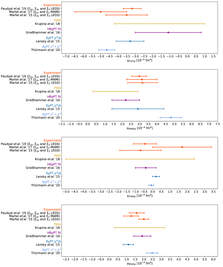
Figure 9: Summary for the lowest-order spin polarizabilities $\gamma_{E1E1p}$, $\gamma_{M1M1p}$, $\gamma_{E1M2p}$ and $\gamma_{M1E2p}$ of the proton. Theoretical predictions from chiral EFT are compared with extractions based on CS data. The experimental results are combinations of different beam asymmetry and double-polarization observable measurements at MAMI and LEGS: $\Sigma_{2x}$ Martel et al. (2017, 2015), $\Sigma_{2z}$ Paudyal et al. (2019) and ${\Sigma}_{3}$ Sokhoyan et al. (2017); Blanpied et al. (2001). Krupina et al. Krupina et al. (2018) performed a PWA of proton RCS data below pion-production threshold.

4 Nucleon Polarizabilities

In the following, I want to discuss the nucleon polarizabilities, focusing on new empirical results from the last five years and comparisons to $\chi$PT predictions. References quoted in the summary figures are: PDG Zyla et al. (2020), MAID Drechsel et al. (2007), experiments Paudyal et al. (2019); Martel et al. (2017); Sokhoyan et al. (2017); Martel et al. (2015); Dutz et al. (2003); Kossert et al. (2003), dispersion relations Schumacher (2019); Pasquini et al. (2019, 2018); Gryniuk et al. (2016); Pasquini et al. (2010); Holstein et al. (2000); Babusci et al. (1998b); Schröder (1980), PWA Krupina et al. (2018), lattice QCD Bignell et al. (2020); Lujan et al. (2016); Hall et al. (2014); Detmold et al. (2010); Engelhardt (2007); Christensen et al. (2005), HB$\chi$PT fit Griesshammer et al. (2016); Myers et al. (2014); McGovern et al. (2013), B$\chi$PT fit Lensky and McGovern (2014), HB$\chi$PT Bernard et al. (1994); Holstein et al. (2000); Nevado and Pineda (2008), B$\chi$PT $\delta$-expansion Lensky et al. (2015, 2014); Alarcón et al. (2020a, b) and B$\chi$PT $\epsilon$-expansion Bernard et al. (2013); Thürmann et al. (2020).

Most recent HB$\chi$PT McGovern et al. (2013); Griesshammer et al. (2012); Myers et al. (2014, 2015); Griesshammer et al. (2016) and B$\chi$PT Lensky and Pascalutsa (2009, 2010); Lensky and McGovern (2014); Lensky et al. (2014, 2015, 2017a); Alarcón et al. (2020a, b) calculations and fits of CS observables employ the $\delta$-expansion power counting. An exception are the works of Bernard et al. Bernard et al. (2013) and Thürmann et al. Thürmann et al. (2020). As one can see from Figure 4 (upper panel), B$\chi$PT predictions for $\delta_{LTp}$ within the $\delta$-expansion Lensky et al. (2014); Alarcón et al. (2020b) or the $\epsilon$-expansion Bernard et al. (2013); Thürmann et al. (2020) deviate substantially, since they include the $\Delta(1232)$ in different ways. In the $\epsilon$-expansion, the longitudinal-transverse polarizability receives a large contribution from diagrams where the photons couple directly to the $\Delta(1232)$ inside a loop. These diagrams are absent in the $\delta$-expansion at $\mathcal{O}(p^{4}/\varDelta)$, thus, there the effect of the $\Delta(1232)$ is small and agrees with the MAID model Drechsel et al. (2007). For the generalized longitudinal-transverse polarizability $\delta_{LTp}(Q^{2})$ a similar $Q^{2}$ evolution is found in both power-counting schemes, see Figure 5 (left panel). Therefore, the discrepancy found for the polarizability $\delta_{LTp}$ at the real-photon point continues as a constant shift for all $Q^{2}$ Alarcón et al. (2020b). Another difference between the B$\chi$PT calculations Lensky et al. (2014); Alarcón et al. (2020b); Bernard et al. (2013); Thürmann et al. (2020) is the implementation of the magnetic-dipole $\mathcal{N}$-to-$\Delta$ transition and the coupling $g_{M}$ Krebs (2019). This “$\delta_{LT}$ puzzle” could soon be resolved by an empirical evaluation based on new data for the proton spin structure function $g_{2}$ from the Jefferson Lab “Spin Physics Program”. A preliminary analysis Sli (2018) favored the $\delta$-expansion power counting Alarcón et al. (2020b), just like the MAID model does, cf. Figures 4 and 5. Note that the $\delta$-expansion results in Refs. Alarcón et al. (2020b) and Lensky et al. (2014) are both $\mathcal{O}(p^{4}/\varDelta)$. They differ by an improved error estimate and inclusion of the Coulomb coupling $g_{C}$ Alarcón et al. (2020b). The $\epsilon$-expansion results in Refs. Bernard et al. (2013) and Thürmann et al. (2020) are $\mathcal{O}(\epsilon^{3})$ and $\mathcal{O}(\epsilon^{3}+p^{4})$, respectively.

Similarly, we observe that the extensive set of empirical evaluations of the generalized forward spin polarizability $\gamma_{0}(Q^{2})$ at $Q^{2}<0.3$ GeV² agrees perfectly with the $\delta$-expansion prediction Alarcón et al. (2020b), but differs from the $\epsilon$-expansion prediction Bernard et al. (2013); Thürmann et al. (2020), cf. Figures 10 and 12 (upper panel). For the higher-order analogue $\bar{\gamma}_{0}(Q^{2})$, shown in Figure 12 (lower panel), the situation is less obvious. Only the dispersive evaluations of $\bar{\gamma}_{0p}$ at the real-photon point, cf. Figure 6, are in slight disagreement with the $\mathcal{O}(p^{4}/\varDelta)$ prediction Alarcón et al. (2020b), while conform with the $\mathcal{O}(\epsilon^{3}+p^{4})$ prediction Thürmann et al. (2020).

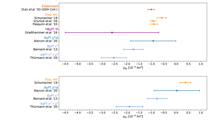
Figure 10: Summary for the forward spin polarizability of the proton $\gamma_{0p}$ (upper panel) and neutron $\gamma_{0n}$ (lower panel). Theoretical predictions from chiral EFT are compared with empirical evaluations of the forward spin polarizability sum rule (36) at the real-photon point.

The most studied polarizabilities are the electric and magnetic dipole polarizabilities, for which the Particle Data Group publishes recommended values Zyla et al. (2020). They are needed as input for calculations of the proton-structure effects in the muonic-hydrogen Lamb shift from two-photon exchange. Of particular importance is $\beta_{M1p}$. It enters the $\overline{T}_{1}(0,Q^{2})$ subtraction function (31), which has to be modeled Birse and McGovern (2012) or predicted within $\chi$PT Alarcón et al. (2020a); Lensky et al. (2018); Peset and Pineda (2014) because it cannot be measured in experiment or reconstructed from the unpolarized proton structure function $f_{1}$ in the dispersive approach, cf. Eq. (28). Recently, $\beta_{M1p}$ has therefore been extracted from the linear polarization beam asymmetry,

$${\Sigma}_{3}=\frac{\mathrm{d}\sigma_{||}-\mathrm{d}\sigma_{\perp}}{\mathrm{d}\sigma_{||}+\mathrm{d}\sigma_{\perp}},$$ (40)

measured for the proton by the A2 Collaboration Sokhoyan et al. (2017) and LEGS Blanpied et al. (2001). Up to $\mathcal{O}(\nu^{2}$), the beam asymmetry ${\Sigma}_{3}$ provides access to $\beta_{M1}$ independent of $\alpha_{E1}$ Krupina and Pascalutsa (2013):

$$\overline{{\Sigma}}_{3}=-\frac{4M_{N}\omega_{B}^{2}\cos\theta_{B}\sin^{2}\theta_{B}}{(1+\cos^{2}\theta_{B})^{2}}\,\alpha^{-1}\beta_{M1}.$$ (41)

Presently, the extraction of $\beta_{M1p}$ from $\Sigma_{3}$ Sokhoyan et al. (2017) is not competitive with the standard dispersive analyses of unpolarized CS cross sections. New high-precision measurements with significantly higher statistics should change this.

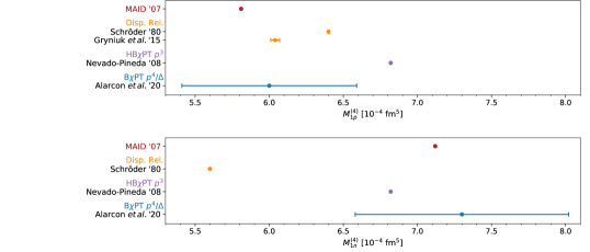
Figure 11: Summary for the fourth-order Baldin sum rule of the proton $M_{1p}^{(4)}$ (upper panel) and neutron $M_{1n}^{(4)}$ (lower panel). Theoretical predictions from chiral EFT are compared with empirical evaluations of the fourth-order Baldin sum rule (32) at the real-photon point.

Analyses of CS data with fixed-$t$ unsubtracted dispersion relations can be found in Refs. Schumacher (2005); Babusci et al. (1998b), with an update in Ref. Schumacher (2019). Fixed-$t$ subtracted dispersion relations are used in Ref. Holstein et al. (2000), and are applied together with a bootstrap-based fitting technique in the recent Ref. Pasquini et al. (2019). Unfortunately, the dispersive and $\chi$PT fits tend to disagree for certain polarizabilities, e.g., for $\alpha_{E1p}$ and $\beta_{M1p}$, cf. Figures 2 and 3 (upper panels). The $\mathcal{O}(p^{4}/\Delta)$ B$\chi$PT prediction Lensky et al. (2015) and the B$\chi$PT fit Lensky and McGovern (2014) of the proton dipole polarizabilities, see Figures 2 and 3 (upper panels), are in good agreement. A HB$\chi$PT fit, which also includes the lowest-order spin polarizabilities in Figures 9 and 10, agrees with the B$\chi$PT results Lensky et al. (2015); Lensky and McGovern (2014) except for $\gamma_{M1E2p}$. Recently, a model-independent PWA of proton RCS data below pion-production threshold has shown Krupina et al. (2018) that the differences between dispersive approaches and B$\chi$PT results are due to inconsistent experimental data subsets, rather than the “model-dependence” of the theoretical frameworks. In the summary figures for the dipole and lowest-order spin polarizabilities, cf. Figures 2, 3 and 9 (upper panels), I show the spread of results from their PWA fits of different data subsets Krupina et al. (2018). Note that all fits use the data-driven evaluations of the Baldin and forward spin polarizability sum rules from Refs. Gryniuk et al. (2016, 2015) as input. Their analysis shows that the difference of proton scalar polarizabilities is constrained to a rather broad interval Krupina et al. (2018): $\alpha_{E1p}-\beta_{M1p}=(6.9\dots 10.9)\times 10^{-4}$fm³. In Ref. Pasquini et al. (2018), the dipole dynamical polarizabilities entering the multipole decomposition of the scattering amplitudes were for the first time extracted from proton RCS data below pion-production threshold. At lowest order, they are related to the static dipole and dispersive polarizabilities, see Figure 8 (upper panel).

Both the partial-wave and the dispersive analysis in Refs. Krupina et al. (2018) and Pasquini et al. (2018) come to the conclusion that quantity and quality of the CS data has to increase for improved extractions of the nucleon polarizabilities. A trend is going towards the measurement of beam asymmetries, such as $\Sigma_{3}$, and double-polarization observables:

$$\Sigma_{2x}={\mathrm{d}\sigma^{R}_{+x}-\mathrm{d}\sigma^{L}_{+x}\over\mathrm{d}\sigma^{R}_{+x}+\mathrm{d}\sigma^{L}_{+x}},$$ (42a)

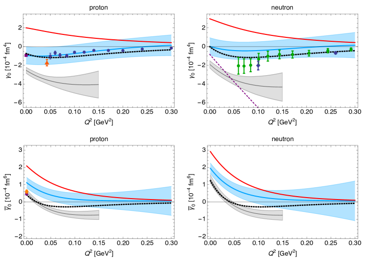
Figure 12: Upper panel: Generalized forward spin polarizability, Eq. (36), for the proton (left) and neutron (right) as function of $Q^{2}$. The black dotted line is the MAID model prediction Drechsel et al. (2001, 1999); Tiator (2020), which is taken from Refs. Drechsel et al. (2003) (proton) and Amarian et al. (2004) (neutron). The red line shows the leading-order B$\chi$PT result. The blue band is the $\mathcal{O}(p^{4}/\Delta)$ B$\chi$PT result from Ref. Alarcón et al. (2020b). The gray band is the $\mathcal{O}(\epsilon^{3}+p^{4})$ B$\chi$PT result from Ref. Thürmann et al. (2020). The purple short-dashed lines is the $\mathcal{O}(p^{4})$ HB results from Ref. Kao et al. (2003); note that the corresponding proton curve is outside of the plotted range. The experimental points for the proton are from: Ref. Prok et al. (2009) (blue dots), Ref. Gryniuk et al. (2016) (purple square) and Ref. Zielinski (2010) (orange triangle; uncertainties added in quadrature). The experimental points for the neutron are from: Ref. Amarian et al. (2004) (blue diamonds) and Ref. Guler et al. (2015) (green dots; statistical and systematic uncertainties added in quadrature). Lower Panel: Fifth-order generalized forward spin polarizability, Eq. (37), for the proton (left) and neutron (right) as function of $Q^{2}$. The black dotted line is the MAID model prediction Drechsel et al. (2007). The experimental points for the proton are from: Ref. Gryniuk et al. (2016) (purple square) and Ref. Pasquini et al. (2010) (orange dot).

$$\Sigma_{2z}={\mathrm{d}\sigma^{R}_{+z}-\mathrm{d}\sigma^{L}_{+z}\over\mathrm{d}\sigma^{R}_{+z}+\mathrm{d}\sigma^{L}_{+z}},$$ (42b)

where $\mathrm{d}\sigma^{R(L)}_{+x}$ and $\mathrm{d}\sigma^{R(L)}_{+z}$ are the differential cross sections for right (left) circularly polarized photons scattering from a nucleon target polarized either in the transverse $+\hat{x}$ direction or in the incident beam direction $+\hat{z}$. Here, the advantage is that systematic uncertainties, e.g., variations in photon flux or uncertainties in target thickness, are canceling out. Combining double-polarization observable and beam-asymmetry measurements, one is sensitive to the lowest-order spin polarizabilities, see Figure 9. For the extraction of the polarizabilities from the MAMI data for $\Sigma_{2x}$ Martel et al. (2017, 2015), $\Sigma_{2z}$ Paudyal et al. (2019) and ${\Sigma}_{3}$ Sokhoyan et al. (2017), as well as the older LEGS data for ${\Sigma}_{3}$ Blanpied et al. (2001), one can use dispersive models Pasquini et al. (2007); Holstein et al. (2000); Drechsel et al. (2003) or $\chi$PT fits Lensky and Pascalutsa (2010).

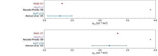
Figure 13: Summary for the longitudinal polarizability of the proton $\alpha_{Lp}$ (upper panel) and neutron $\alpha_{Ln}$ (lower panel). Theoretical predictions from chiral EFT are compared with the MAID unitary isobar model.

Besides experimental efforts, lattice QCD is making considerable progress. Most notably are the lattice QCD predictions for $\beta_{M1}$ with chiral extrapolation to physical pion mass Bignell et al. (2018, 2020), as well as the plentiful results for $\alpha_{E1n}$ Lujan et al. (2016); Detmold et al. (2010); Engelhardt (2007); Christensen et al. (2005). By now, even direct lattice evaluations of the unpolarized forward VVCS amplitudes became possible and can be used to determine the structure functions and their moments Hannaford-Gunn et al. (2020); Chambers et al. (2017); Can et al. (2020).

In Figures 4, 6, 10, 11, 13, one can see updated results from the recent $\mathcal{O}(p^{4}/\Delta)$ B$\chi$PT prediction of unpolarized VVCS Alarcón et al. (2020a), related to $\alpha_{L}$ and $M_{1}^{(4)}$, and polarized VVCS Alarcón et al. (2020b), related to $\delta_{LT}$, $\gamma_{0}$ and $\bar{\gamma}_{0}$. The latter could be compared to new results from the Jefferson Lab “Spin Physics Program” for the proton spin structure functions $g_{1}$ and $g_{2}$, see for instance the E08-027 experiment Zielinski (2010) and the E97-110 experiment Sulkosky et al. (2020). Note that the HB$\chi$PT predictions for $M_{1}^{(4)}$ and $\alpha_{L}$ shown in Figures 11 and 13 were extracted from the VVCS amplitudes presented in Ref. Nevado and Pineda (2008), but are not quoted in the original work.

5 Conclusion and Outlook

The chiral EFT expansion for nucleon polarizabilities begins with inverse powers of pion mass and other light scales, such as the nucleon-$\Delta$ mass difference. These inverse powers ($1/m_{\pi}$, $1/\varDelta$, etc.) along with the chiral logs constitute predictions of $\chi$PT. As such, the polarizabilities, and, in fact, the entire process of CS at low energies, provide a testing ground for $\chi$PT.

Moreover, the interpretation of low-energy CS data and the extraction of nucleon polarizabilities therefrom should rely on a systematic theoretical framework such as $\chi$PT. In what we have seen thus far, $\chi$PT is quite successful in the prediction of nucleon polarizabilities. It can as well be used to design “optimal” future experiments for improving the empirical determinations of nucleon polarizabilities Melendez et al. (2020).

An alternative to $\chi$PT, in the field of nucleon CS, is provided by models based on fixed-$t$ dispersion relations L’vov et al. (1997); Drechsel et al. (2000). The theoretical uncertainties of the dispersive approach are harder to understand, but, at least within the quoted uncertainties, the extracted values of polarizabilities are in overall comparable to those found in $\chi$PT. However, a few discrepancies remain. For example, the tension in the value of the proton magnetic dipole polarizability still persists, cf. “Disp. Rel.” vs. $\chi$PT results in Figure 3 (upper panel). A model-independent PWA shows Krupina et al. (2018) that this discrepancy is likely to be caused by the experimental CS database, rather than the differences between the theoretical frameworks. With MAMI Mornacchi (2019) and HIGS Ahmed (2020) experiments underway, the database will soon be greatly improved. It is worth mentioning that MAMI is also finalising a program to measure the CS double-polarization observables ($\Sigma_{2x}$, $\Sigma_{2z}$) which will lead to an improved extraction of proton spin polarizabilities Martel et al. (2017, 2015); Paudyal et al. (2019).

Even among the various $\chi$PT calculations there are significant discrepancies that need to be understood. The differences between the heavy-baryon (HB$\chi$PT) and the Lorentz-invariant covariant (B$\chi$PT) results are not difficult to track. However, differences among various B$\chi$PT calculations are more troublesome. A prominent example is the longitudinal-transverse polarizability of the proton (upper panel of Figure 4 and left panel of Figure 5), where the $\delta$- and $\epsilon$-expansion B$\chi$PT calculations are different by about a factor of 2. This “$\delta_{LT}$ puzzle” could soon receive an experimental resolution, when the long-promised data from Jefferson Lab “Spin Physics Program” Zielinski (2010); Adhikari et al. (2018); Sulkosky et al. (2020) on the proton spin structure function $g_{2}$ will be published Sli (2018). Besides the polarizabilities, the Gerasimov–Drell–Hearn sum rule for the neutron will be verified by the E97-110 experiment using a helium-3 target Ton (2019).

In the mean time, lattice QCD calculations of nucleon polarizabilities are advancing towards the physical pion mass. Until now, however, $\chi$PT has been used to extrapolate the lattice results to the physical mass Bignell et al. (2020); Hall et al. (2014). A significant progress has recently been achieved in calculating the proton polarizabilities Bignell et al. (2020); Detmold et al. (2010), and in direct calculations of the spin-independent forward VVCS Hannaford-Gunn et al. (2020); Chambers et al. (2017); Can et al. (2020).

In the next few years, one can expect a lot of progress in this field, mainly due to the upcoming data from MAMI, HIGS and Jefferson Lab. New $\chi$PT and lattice QCD calculations will certainly continue to advance and will, hopefully, bring some clarity on the aforementioned discrepancies.

Financial support from the Swiss National Science Foundation is gratefully acknowledged.

References

- Pagels (1975) H. Pagels, Phys. Rept. 16, 219 (1975).
- Weinberg (1979) S. Weinberg, Physica A 96, 327 (1979).
- Gasser and Leutwyler (1984) J. Gasser and H. Leutwyler, Ann. Phys. 158, 142 (1984).
- Gasser et al. (1988) J. Gasser, M. E. Sainio, and A. Švarc, Nucl. Phys. B 307, 779 (1988).
- Bernard et al. (1991) V. Bernard, N. Kaiser, and U.-G. Meißner, Phys. Rev. Lett. 67, 1515 (1991).
- Bernard et al. (1992) V. Bernard, N. Kaiser, and U.-G. Meißner, Nucl. Phys. B 373, 346 (1992).
- Baldin (1960) A. M. Baldin, Nucl. Phys. 18, 310 (1960).
- Lapidus (1962) L. I. Lapidus, Zh. Eksp. Teor. Fiz. 43, 1358 (1962), [Sov. Phys. JETP 16, 964 (1963)].
- Pascalutsa (2018) V. Pascalutsa, Causality Rules, IOP Concise Physics (IOP Publishing and Morgan & Claypool Publishers, 2018).
- Damashek and Gilman (1970) M. Damashek and F. J. Gilman, Phys. Rev. D 1, 1319 (1970).
- Schröder (1980) U. Schröder, Nucl. Phys. B 166, 103 (1980).
- Babusci et al. (1998a) D. Babusci, G. Giordano, and G. Matone, Phys. Rev. C 57, 291 (1998a), arXiv:nucl-th/9710017 .
- Levchuk and L’vov (2000) M. I. Levchuk and A. I. L’vov, Nucl. Phys. A 674, 449 (2000), nucl-th/9909066 .
- Olmos de León et al. (2001) V. Olmos de León et al., Eur. Phys. J. A 10, 207 (2001).
- Gryniuk et al. (2015) O. Gryniuk, F. Hagelstein, and V. Pascalutsa, Phys. Rev. D 92, 074031 (2015), arXiv:1508.07952 [nucl-th] .
- Pohl et al. (2010) R. Pohl et al., Nature 466, 213 (2010).
- Antognini et al. (2013) A. Antognini, F. Nez, K. Schuhmann, F. D. Amaro, et al., Science 339, 417 (2013).
- Pohl et al. (2017) R. Pohl et al., Proceedings, 12th International Conference on Low Energy Antiproton Physics (LEAP2016), Kanazawa, Japan, March 6-11, 2016, JPS Conf. Proc. 18, 011021 (2017), arXiv:1609.03440 [physics.atom-ph] .
- Bakalov et al. (2015) D. Bakalov, A. Adamczak, M. Stoilov, and A. Vacchi, Proceedings, 5th International Conference on Exotic Atoms and Related Topics (EXA2014): Vienna, Austria, September 15-19, 2014, Hyperfine Interact. 233, 97 (2015).
- Kanda et al. (2018) S. Kanda et al., J. Phys. Conf. Ser. 1138, 012009 (2018).
- Alarcón et al. (2014) J. M. Alarcón, V. Lensky, and V. Pascalutsa, Eur. Phys. J. C 74, 2852 (2014), arXiv:1312.1219 [hep-ph] .
- Hagelstein and Pascalutsa (2016) F. Hagelstein and V. Pascalutsa, PoS CD15, 077 (2016), arXiv:1511.04301 [nucl-th] .
- Hagelstein (2017) F. Hagelstein, Exciting Nucleons in Compton Scattering and Hydrogen-Like Atoms, Ph.D. thesis, Mainz U., Inst. Kernphys. (2017), arXiv:1710.00874 [nucl-th] .
- Hagelstein et al. (2016) F. Hagelstein, R. Miskimen, and V. Pascalutsa, Prog. Part. Nucl. Phys. 88, 29 (2016).
- Lensky and Pascalutsa (2019) V. Lensky and V. Pascalutsa, PoS CD2018, 035 (2019), arXiv:1907.09024 [hep-ph] .
- Guichon and Vanderhaeghen (1998) P. A. M. Guichon and M. Vanderhaeghen, Prog. Part. Nucl. Phys. 41, 125 (1998), hep-ph/9806305 .
- Fonvieille et al. (2020) H. Fonvieille, B. Pasquini, and N. Sparveris, Prog. Part. Nucl. Phys. 113, 103754 (2020).
- Drechsel et al. (2003) D. Drechsel, B. Pasquini, and M. Vanderhaeghen, Phys. Rept. 378, 99 (2003), hep-ph/0212124 .
- Pasquini and Vanderhaeghen (2018) B. Pasquini and M. Vanderhaeghen, Ann. Rev. Nucl. Part. Sci. 68, 75 (2018), arXiv:1805.10482 [hep-ph] .
- Pascalutsa et al. (2007) V. Pascalutsa, M. Vanderhaeghen, and S. N. Yang, Phys. Rept. 437, 125 (2007), arXiv:hep-ph/0609004 .
- Phillips (2009) D. R. Phillips, J. Phys. G 36, 104004 (2009), arXiv:0903.4439 [nucl-th] .
- Griesshammer et al. (2012) H. Griesshammer, J. McGovern, D. Phillips, and G. Feldman, Prog. Part. Nucl. Phys. 67, 841 (2012), arXiv:1203.6834 [nucl-th] .
- Holstein and Scherer (2014) B. R. Holstein and S. Scherer, Ann. Rev. Nucl. Part. Sci. 64, 51 (2014), arXiv:1401.0140 [hep-ph] .
- Geng (2013) L. Geng, Front. Phys. China 8, 328 (2013), arXiv:1301.6815 [nucl-th] .
- Deur et al. (2019) A. Deur, S. J. Brodsky, and G. F. De Téramond, Rept. Prog. Phys. 82 (2019), arXiv:1807.05250 [hep-ph] .
- Scherer and Schindler (2012) S. Scherer and M. R. Schindler, A Primer for Chiral Perturbation Theory (Springer Berlin / Heidelberg, 2012).
- Gegelia and Japaridze (1999) J. Gegelia and G. Japaridze, Phys. Rev. D 60, 114038 (1999), arXiv:hep-ph/9908377 .
- Fuchs et al. (2003) T. Fuchs, J. Gegelia, G. Japaridze, and S. Scherer, Phys. Rev. D 68, 056005 (2003), arXiv:hep-ph/0302117 .
- Lensky and Pascalutsa (2009) V. Lensky and V. Pascalutsa, Pisma Zh. Eksp. Teor. Fiz. 89, 127 (2009), [JETP Lett. 89 (2009) 108], arXiv:0803.4115 [nucl-th] .
- Lensky and Pascalutsa (2010) V. Lensky and V. Pascalutsa, Eur. Phys. J. C 65, 195 (2010).
- Lensky et al. (2015) V. Lensky, J. McGovern, and V. Pascalutsa, Eur. Phys. J. C 75, 604 (2015), arXiv:1510.02794 [hep-ph] .
- Lensky et al. (2017a) V. Lensky, V. Pascalutsa, and M. Vanderhaeghen, Eur. Phys. J. C 77, 119 (2017a), arXiv:1612.08626 [hep-ph] .
- Lensky et al. (2014) V. Lensky, J. M. Alarcón, and V. Pascalutsa, Phys. Rev. C 90, 055202 (2014), arXiv:1407.2574 [hep-ph] .
- Alarcón et al. (2020a) J. M. Alarcón, F. Hagelstein, V. Lensky, and V. Pascalutsa, Phys. Rev. D 102, 014006 (2020a).
- Alarcón et al. (2020b) J. M. Alarcón, F. Hagelstein, V. Lensky, and V. Pascalutsa, hep-ph/2006.08626 (2020b).
- Ledwig et al. (2012) T. Ledwig, J. Martin-Camalich, V. Pascalutsa, and M. Vanderhaeghen, Phys. Rev. D 85, 034013 (2012), arXiv:1108.2523 [hep-ph] .
- Colangelo et al. (2001) G. Colangelo, J. Gasser, and H. Leutwyler, Nucl. Phys. B 603, 125 (2001), arXiv:hep-ph/0103088 [hep-ph] .
- Caprini et al. (2006) I. Caprini, G. Colangelo, and H. Leutwyler, QCD and hadronic physics. Proceedings, International Conference, Beijing, China, June 16-20, 2005, Int. J. Mod. Phys. A 21, 954 (2006), arXiv:hep-ph/0509266 [hep-ph] .
- Pascalutsa and Vanderhaeghen (2005a) V. Pascalutsa and M. Vanderhaeghen, Phys. Rev. Lett. 95, 232001 (2005a), arXiv:hep-ph/0508060 .
- Pascalutsa and Vanderhaeghen (2006a) V. Pascalutsa and M. Vanderhaeghen, Phys. Rev. D 73, 034003 (2006a), arXiv:hep-ph/0512244 .
- Patrignani et al. (2016) C. Patrignani et al. (Particle Data Group), Chin. Phys. C 40, 100001 (2016).
- Pascalutsa and Vanderhaeghen (2005b) V. Pascalutsa and M. Vanderhaeghen, Phys. Rev. Lett. 94, 102003 (2005b), arXiv:nucl-th/0412113 .
- Pascalutsa and Vanderhaeghen (2006b) V. Pascalutsa and M. Vanderhaeghen, Phys. Lett. B 636, 31 (2006b), arXiv:hep-ph/0511261 .
- Hemmert et al. (1997a) T. R. Hemmert, B. R. Holstein, and J. Kambor, Phys. Lett. B 395, 89 (1997a), arXiv:hep-ph/9606456 [hep-ph] .
- Pascalutsa and Phillips (2003) V. Pascalutsa and D. R. Phillips, Phys. Rev. C 67, 055202 (2003), arXiv:nucl-th/0212024 .
- Bernard et al. (2013) V. Bernard, E. Epelbaum, H. Krebs, and U.-G. Meißner, Phys. Rev. D 87, 054032 (2013).
- McGovern et al. (2013) J. A. McGovern, D. R. Phillips, and H. W. Grießhammer, Eur. Phys. J. A 49, 12 (2013).
- Lensky and McGovern (2014) V. Lensky and J. A. McGovern, Phys. Rev. C 89, 032202 (2014), arXiv:1401.3320 [nucl-th] .
- Myers et al. (2014) L. Myers et al. (COMPTON@MAX-lab), Phys. Rev. Lett. 113, 262506 (2014), arXiv:1409.3705 [nucl-ex] .
- Myers et al. (2015) L. S. Myers et al., Phys. Rev. C 92, 025203 (2015), arXiv:1503.08094 [nucl-ex] .
- Griesshammer et al. (2016) H. W. Griesshammer, J. A. McGovern, and D. R. Phillips, Eur. Phys. J. A 52, 139 (2016).
- Jenkins and Manohar (1991) E. E. Jenkins and A. V. Manohar, Phys. Lett. B 255, 558 (1991).
- Butler and Savage (1992) M. N. Butler and M. J. Savage, Phys. Lett. B 294, 369 (1992), arXiv:hep-ph/9209204 [hep-ph] .
- Bernard et al. (1995) V. Bernard, N. Kaiser, and U.-G. Meißner, Int. J. Mod. Phys. E 4, 193 (1995), arXiv:hep-ph/9501384 .
- Hemmert et al. (1997b) T. R. Hemmert, B. R. Holstein, and J. Kambor, Phys. Rev. D 55, 5598 (1997b), arXiv:hep-ph/9612374 .
- Hildebrandt et al. (2004) R. P. Hildebrandt, H. W. Grießhammer, T. R. Hemmert, and B. Pasquini, Eur. Phys. J. A 20, 293 (2004).
- Kao et al. (2003) C. W. Kao, T. Spitzenberg, and M. Vanderhaeghen, Phys. Rev. D 67, 016001 (2003).
- Kao et al. (2004) C.-W. Kao, D. Drechsel, S. Kamalov, and M. Vanderhaeghen, Phys. Rev. D 69, 056004 (2004).
- Nevado and Pineda (2008) D. Nevado and A. Pineda, Phys. Rev. C 77, 035202 (2008), arXiv:0712.1294 [hep-ph] .
- Hall and Pascalutsa (2012) J. M. Hall and V. Pascalutsa, Eur. Phys. J. C 72, 2206 (2012), arXiv:1203.0724 [hep-ph] .
- Drechsel et al. (2001) D. Drechsel, S. S. Kamalov, and L. Tiator, Phys. Rev. D 63, 114010 (2001), arXiv:hep-ph/0008306 .
- Drechsel et al. (1999) D. Drechsel, O. Hanstein, S. S. Kamalov, and L. Tiator, Nucl. Phys. A 645, 145 (1999), arXiv:nucl-th/9807001 .
- Thürmann et al. (2020) M. Thürmann, E. Epelbaum, A. Gasparyan, and H. Krebs, nucl-th/2007.08438 (2020).
- Amarian et al. (2004) M. Amarian et al. (Jefferson Lab E94010), Phys. Rev. Lett. 93, 152301 (2004), arXiv:nucl-ex/0406005 [nucl-ex] .
- Hearn and Leader (1962) A. C. Hearn and E. Leader, Phys. Rev. 126, 789 (1962).
- Babusci et al. (1998b) D. Babusci, G. Giordano, A. L’vov, G. Matone, and A. Nathan, Phys. Rev. C 58, 1013 (1998b).
- Lensky et al. (2018) V. Lensky, F. Hagelstein, V. Pascalutsa, and M. Vanderhaeghen, Phys. Rev. D 97, 074012 (2018).
- Pascalutsa and Vanderhaeghen (2015) V. Pascalutsa and M. Vanderhaeghen, Phys. Rev. D 91, 051503 (R) (2015), arXiv:1409.5236 [nucl-th] .
- Lensky et al. (2017b) V. Lensky, V. Pascalutsa, M. Vanderhaeghen, and C. Kao, Phys. Rev. D 95, 074001 (2017b).
- Hemmert et al. (1998) T. R. Hemmert, B. R. Holstein, J. Kambor, and G. Knochlein, Phys. Rev. D 57, 5746 (1998).
- Low (1954) F. E. Low, Phys. Rev. 96, 1428 (1954).
- Gell-Mann and Goldberger (1954) M. Gell-Mann and M. L. Goldberger, Phys. Rev. 96, 1433 (1954).
- Gilman (1968) F. J. Gilman, Phys. Rev. 167, 1365 (1968).
- Drechsel et al. (1998) D. Drechsel, G. Knochlein, A. Korchin, A. Metz, and S. Scherer, Phys. Rev. C 58, 1751 (1998), arXiv:nucl-th/9804078 .
- Beričič et al. (2019) J. Beričič et al. (A1), Phys. Rev. Lett. 123, 192302 (2019), arXiv:1907.09954 [nucl-ex] .
- Guiasu and Radescu (1979) I. Guiasu and E. Radescu, Annals Phys. 120, 145 (1979).
- Holstein et al. (2000) B. R. Holstein, D. Drechsel, B. Pasquini, and M. Vanderhaeghen, Phys. Rev. C 61, 034316 (2000).
- Pasquini et al. (2018) B. Pasquini, P. Pedroni, and S. Sconfietti, Phys. Rev. C 98, 015204 (2018), arXiv:1711.07401 [hep-ph] .
- Gerasimov (1966) S. Gerasimov, Sov. J. Nucl. Phys. 2, 430 (1966).
- Drell and Hearn (1966) S. Drell and A. C. Hearn, Phys. Rev. Lett. 16, 908 (1966).
- Ahrens et al. (2001) J. Ahrens et al. (GDH, A2), Phys. Rev. Lett. 87, 022003 (2001), arXiv:hep-ex/0105089 .
- Helbing (2002) K. Helbing (GDH), Nucl. Phys. Proc. Suppl. 105, 113 (2002).
- Martel et al. (2017) P. Martel, M. Biroth, C. Collicott, D. Paudyal, and A. Rajabi (A2), EPJ Web Conf. 142, 01021 (2017).
- Martel et al. (2015) P. P. Martel et al. (A2), Phys. Rev. Lett. 114, 112501 (2015), arXiv:1408.1576 [nucl-ex] .
- Paudyal et al. (2019) D. Paudyal et al. (A2), nucl-ex/1909.02032 (2019), arXiv:1909.02032 [nucl-ex] .
- Sokhoyan et al. (2017) V. Sokhoyan et al., Eur. Phys. J. A 53, 14 (2017), arXiv:1611.03769 [nucl-ex] .
- Blanpied et al. (2001) G. Blanpied et al., Phys. Rev. C 64, 025203 (2001).
- Krupina et al. (2018) N. Krupina, V. Lensky, and V. Pascalutsa, Phys. Lett. B 782, 34 (2018), arXiv:1712.05349 [nucl-th] .
- Zyla et al. (2020) P. A. Zyla et al., Prog. Theor. Exp. Phys. 083C01 (2020).
- Drechsel et al. (2007) D. Drechsel, S. Kamalov, and L. Tiator, Eur. Phys. J. A, 69 (2007), maid.kph.uni-mainz.de.
- Dutz et al. (2003) H. Dutz et al. (GDH), Phys. Rev. Lett. 91, 192001 (2003).
- Kossert et al. (2003) K. Kossert et al., Eur. Phys. J. A 16, 259 (2003), arXiv:nucl-ex/0210020 .
- Schumacher (2019) M. Schumacher, LHEP 4, 4 (2019), arXiv:1907.05434 [hep-ph] .
- Pasquini et al. (2019) B. Pasquini, P. Pedroni, and S. Sconfietti, J. Phys. G 46, 104001 (2019), arXiv:1903.07952 [hep-ph] .
- Gryniuk et al. (2016) O. Gryniuk, F. Hagelstein, and V. Pascalutsa, Phys. Rev. D 94, 034043 (2016), arXiv:1604.00789 [nucl-th] .
- Pasquini et al. (2010) B. Pasquini, P. Pedroni, and D. Drechsel, Phys. Lett. B 687, 160 (2010), arXiv:1001.4230 [hep-ph] .
- Bignell et al. (2020) R. Bignell, W. Kamleh, and D. Leinweber, Phys. Rev. D 101, 094502 (2020), arXiv:2002.07915 [hep-lat] .
- Lujan et al. (2016) M. Lujan, A. Alexandru, W. Freeman, and F. Lee, Phys. Rev. D 94, 074506 (2016), arXiv:1606.07928 [hep-lat] .
- Hall et al. (2014) J. M. M. Hall, D. B. Leinweber, and R. D. Young, Phys. Rev. D 89, 054511 (2014), arXiv:1312.5781 [hep-lat] .
- Detmold et al. (2010) W. Detmold, B. Tiburzi, and A. Walker-Loud, Phys. Rev. D 81, 054502 (2010), arXiv:1001.1131 [hep-lat] .
- Engelhardt (2007) M. Engelhardt (LHPC), Phys. Rev. D 76, 114502 (2007), arXiv:0706.3919 [hep-lat] .
- Christensen et al. (2005) J. C. Christensen, W. Wilcox, F. X. Lee, and L. Zhou, Phys. Rev. D 72, 034503 (2005).
- Bernard et al. (1994) V. Bernard, N. Kaiser, U. G. Meissner, and A. Schmidt, Z. Phys. A 348, 317 (1994), arXiv:hep-ph/9311354 .
- Krebs (2019) H. Krebs, PoS CD2018, 031 (2019).
- Sli (2018) K. Slifer, talk at the ECT* conference: “Nucleon Spin Structure at Low Q: A Hyperfine View" (2018).
- Birse and McGovern (2012) M. C. Birse and J. A. McGovern, Eur. Phys. J. A 48, 120 (2012), arXiv:1206.3030 [hep-ph] .
- Peset and Pineda (2014) C. Peset and A. Pineda, Nucl. Phys. B 887, 69 (2014), arXiv:1406.4524 [hep-ph] .
- Krupina and Pascalutsa (2013) N. Krupina and V. Pascalutsa, Phys. Rev. Lett. 110, 262001 (2013).
- Schumacher (2005) M. Schumacher, Prog. Part. Nucl. Phys. 55, 567 (2005), arXiv:hep-ph/0501167 .
- Tiator (2020) L. Tiator, “private communication,” (2020).
- Prok et al. (2009) Y. Prok et al. (CLAS), Phys. Lett. B 672, 12 (2009), arXiv:0802.2232 [nucl-ex] .
- Zielinski (2010) R. Zielinski, The g2p Experiment: A Measurement of the Proton’s Spin Structure Functions, Ph.D. thesis, New Hampshire U. (2010), arXiv:1708.08297 [nucl-ex] .
- Guler et al. (2015) N. Guler et al. (CLAS), Phys. Rev. C 92, 055201 (2015), arXiv:1505.07877 [nucl-ex] .
- Pasquini et al. (2007) B. Pasquini, D. Drechsel, and M. Vanderhaeghen, Phys. Rev. C 76, 015203 (2007), arXiv:0705.0282 [hep-ph] .
- Bignell et al. (2018) R. Bignell, J. Hall, W. Kamleh, D. Leinweber, and M. Burkardt, Phys. Rev. D 98, 034504 (2018).
- Hannaford-Gunn et al. (2020) A. Hannaford-Gunn, R. Horsley, Y. Nakamura, H. Perlt, P. Rakow, G. Schierholz, K. Somfleth, H. Stüben, R. Young, and J. Zanotti, in 37th International Symposium on Lattice Field Theory, hep-lat/2001.05090 (2020) arXiv:2001.05090 [hep-lat] .
- Chambers et al. (2017) A. Chambers, R. Horsley, Y. Nakamura, H. Perlt, P. Rakow, G. Schierholz, A. Schiller, K. Somfleth, R. Young, and J. Zanotti, Phys. Rev. Lett. 118, 242001 (2017), arXiv:1703.01153 [hep-lat] .
- Can et al. (2020) K. Can et al., hep-lat/2007.01523 (2020).
- Sulkosky et al. (2020) V. Sulkosky et al. (Jefferson Lab E97-110), Phys. Lett. B 805, 135428 (2020), arXiv:1908.05709 [nucl-ex] .
- Melendez et al. (2020) J. Melendez, R. Furnstahl, H. Grießhammer, J. McGovern, D. Phillips, and M. Pratola, nucl-th/2004.11307 (2020).
- L’vov et al. (1997) A. I. L’vov, V. A. Petrun’kin, and M. Schumacher, Phys. Rev. C 55, 359 (1997).
- Drechsel et al. (2000) D. Drechsel, M. Gorchtein, B. Pasquini, and M. Vanderhaeghen, Phys. Rev. C 61, 015204 (2000).
- Mornacchi (2019) E. Mornacchi (A2), EPJ Web Conf. 199, 05020 (2019).
- Ahmed (2020) M. W. Ahmed, PoS CD2018, 001 (2020).
- Adhikari et al. (2018) K. Adhikari et al. (CLAS), Phys. Rev. Lett. 120, 062501 (2018), arXiv:1711.01974 [nucl-ex] .
- Ton (2019) N. Ton (Small Angle Gdh), PoS CD2018, 044 (2019).