Abstract

According to the Ryu-Takayanagi prescription, the entanglement entropy of subsystems in the boundary conformal field theory (CFT) is proportional to the area of extremal surfaces in bulk asymptotically Anti-de Sitter (AdS) spacetimes. The flat-space limit of these surfaces is not well defined in the generic case. We introduce a new curve in the three-dimensional asymptotically AdS spacetimes with a well-defined flat-space limit. We find this curve by using a new vector, which is vanishing on it and is normal to the bulk modular flow of the original interval in the two-dimensional CFT. The flat-space limit of this new vector is well defined and gives rise to the bulk modular flow of the corresponding asymptotically flat spacetime. Moreover, after Rindler transformation, this new vector is the normal Killing vector of the BTZ inner horizon. We reproduce all known results about the holographic entanglement entropy of Bondi-Metzner-Sachs invariant field theories, which are dual to the asymptotically flat spacetimes.

1 Introduction

One of the proposals for the holographic dual of asymptotically flat spacetimes is given by Bagchi:2010zz,Bagchi:2012cy,[0]Ref. [1, 2]. According to this proposal, the flat-space limit in the gravity side in the context of AdS/CFT corresponds to taking the ultrarelativistic limit in the field theory side. For the two dimensional conformal field theories (CFTs), the ultrarelativistic limit of conformal algebra is performed using the Inonu-Wigner contraction and imposing the vanishing speed of light limit. The resultant algebra, in this case, is infinite dimensional, and it is known as Carroll algebra Leblond65,Duval:2014uoa,[0]Ref. [3, 4]. This two-dimensional ultrarelativistic algebra is isomorphic to a three-dimensional relativistic algebra, which is asymptotic symmetry of asymptotically flat spacetimes at null infinity Barnich:2006av,[0]Ref. [5]. The asymptotic symmetry of four-dimensional asymptotically flat spacetimes is known from a long time ago by the works of Bondi, Metzner, and also Sachs, and this symmetry is known as BMS symmetry BMS,[0]Ref. [6]. Recent progress in this way by Barnich et al. Barnich:2006av,Barnich:4dBMS,aspects,[0]Ref. [5, 7, 8] shows that by imposing nonglobal invariance of symmetry algebra (which was absent in the first formulation of $bms_{4}$ algebra in BMS,[0]Ref. [6] and $bms_{3}$ algebra in Ashtekar:1996cd,[0]Ref. [9]), one can obtain infinite-dimensional algebras in both three- and four-dimensional asymptotically flat spacetimes, which are an extension of translation and rotation of Poincaré algebra. In this view, both of $bms_{3}$ and $bms_{4}$ consist of supertranslations and superrotations.

The isomorphism between two-dimensional Carroll algebra and three-dimensional BMS algebra was the motivation of Bagchi:2010zz,Bagchi:2012cy,[0]Ref. [1, 2] to propose that the holographic dual of asymptotically flat spacetimes are indeed BMS-invariant field theories (BMSFT). BMSFTs are ultrarelativistic theories in one-dimensional lower spacetimes characterized by their infinite-dimensional symmetry algebra. In this paper, we call this correspondence flat/BMSFT. The infinite-dimensional symmetry of BMSFTs provides some universal properties which are independent of the detail of these theories. In this view, one can study the flat-space holography by just using the universal properties of BMSFTs For recent progress in aspects of BMSFTs, see Bagchi:2019xfx,Bagchi:2019clu,[0]Ref. [10, 11].

There are two approaches to improve the dictionary of flat/BMSFT. One is to study BMSFTs directly and relates its observable to the properties of asymptotically flat spacetimes. Another is to start from AdS/CFT and take a limit from its dictionary. In the bulk side, this limit is simply the flat-space limit or zero cosmological constant limit, which applies by taking the limit of Anti-de Sitter (AdS) radius, $\ell$, to infinity.

In this paper, we focus on the second approach to study the holographic entanglement entropy of BMSFTs. because of the infinite-dimensional symmetry of two-dimensional BMSFTs, a universal formula has been proposed for the entanglement entropy in these theories Bagchi:2014iea,[0]Ref. [12]. Later, Jiang:2017ecm,[0]Ref. [13] proposed a holographic description for the BMSFTs entanglement entropy. This holographic description of entanglement entropy is very similar to Ryu and Takayanagi’s (RT) proposal in the context of AdS/CFT Ryu:2006bv,[0]Ref. [14], which associates the dual field theory entanglement entropy to the length of some extremal curves inside the gravitational theory. In the original RT proposal for the asymptotically AdS spacetime, this curve is a geodesic with extremized length anchored to the end points of the interval at the boundary. In the flat/BMSFT correspondence, this curve is also a geodesic with extremized length, but it connects to two null rays emitted from null infinity where end points of the interval lie. Thus in the flat case, the extremal curves are not connected to the dual field theory intervals directly, and this makes finding them a bit tedious and ambiguous.

The method of Jiang:2017ecm,[0]Ref. [13] for constructing extremal curves in asymptotically flat spacetimes is based on Rindler transformation Faulkner:2013ica,[0]Ref. [15]. In the field theory side, this unitary transformation is part of the symmetry of the theory, which relates the original entanglement entropy to a thermal entropy. The thermal entropy corresponds to the entropy (area) of an event horizon in the gravitational theory. The spacetime, in which this event horizon exists, is given by the bulk Rindler transformation from original spacetime. The extremal curve in the original bulk spacetime is nothing but the inverse Rindler transformation of the final event horizon. Thus in this method, one needs to find Rindler transformation and its bulk extension for finding extremal curves. In this view, we do not need to extremize any length, and the extremal curve is a result of Rindler transformation. Although this method applies to all field theories, finding corresponding Rindler transformation is not straightforward.

In the original RT proposal in the context of AdS/CFT, it is not necessary to know Rindler transformation. Imposing extremality conditions for the length of bulk geodesics anchored to the end points of the boundary interval is enough to determine the RT curve. One can interpret the flat-space limit of these curves as the holographic entanglement entropy related to BMSFTs. However, the flat-space limit of these curves is not well defined. The simplicity of the extremization procedure, which is used in the AdS/CFT case, is tedious enough to make someone think about the extremal curves with a well-defined flat-space limit. In this paper, we focus on this problem and introduce a new curve in the asymptotically AdS spacetimes whose flat-space limit yields the results of Jiang:2017ecm,[0]Ref. [13].

The main idea in the current calculation is related to the observation of Fareghbal:2014qga,[0]Ref. [16] and Riegler:2014bia,[0]Ref. [17] that the entropy of flat-space cosmological solution (FSC) which is given by taking the flat-space limit from the BTZ black hole Cornalba:2002fi,[0]Ref. [18] Barnich:2012xq,[0]Ref. [21], is a result of flat-space limit performed on the entropy of BTZ inner horizon. After Rindler transformation, the RT extremal curve transforms into the outer horizon of the corresponding black hole, whereas the curve with a well-defined flat-space limit transforms to the inner horizon.

To bypass Rindler transformation and introduce a method that solely uses the extremality condition, we use the bulk modular flow of the corresponding interval in the AdS case. It vanishes on the RT extremal curve and transforms into the Killing vector normal to the outer horizon after Rindler transformation. The fact that our new curve relates to the inner horizon reveals that the Killing vector normal to the inner horizon can be meaningful in the original coordinate if we apply the inverse Rindler transformation. The interesting point is that the Killing vectors normal to inner and outer horizons are perpendicular to each other, and the sum of their norms is constant. Thus, besides the Killing equation, we have two other equations that associate two vector fields to each other in any coordinate system. One of these vector fields is the bulk modular flow of the original coordinate in the AdS case, and the second one is a new vector field that has a well-defined flat-space limit. The flat-space limit of our new vector field in the asymptotically AdS spacetime yields the bulk modular flow of the corresponding interval introduced in Jiang:2017ecm,[0]Ref. [13] for BMSFT. The interesting point is that the components of the new vector field vanish on the new extremal curve. In other words, this new curve consists of the fixed points of the new vector. Thus, we can bypass Rindler transformation in this way by starting from the bulk modular flow of the original interval in the AdS case and constructing a new vector field by using the Killing equations, normality condition, and norm condition. These equations determine our new vector field. Then, we can take the flat-space limit and find the bulk modular flow of the asymptotically flat case and finally obtain the extremal curve introduced in Jiang:2017ecm,[0]Ref. [13].

In the holographic description proposed for the entanglement entropy of BMSFT introduced in Jiang:2017ecm,[0]Ref. [13], besides an extremal spacelike curve, two null curves are starting from null infinity from end points of the BMSFT interval and intersect the extremal curve. This is the length of the extremal curve bounded between two intersections by null curves that is proportional to the BMSFT entanglement entropy. In this paper, we also propose two new null curves in the asymptotically AdS spacetimes, which their flat-space limit results in the null rays of Jiang:2017ecm,[0]Ref. [13]. The fact that our new curve gets to the boundary at points which are different than the end points of the required interval makes it possible to find null rays that connect end points of the interval to the new curve. However, the number of these null geodesics is infinite. We observe that imposing the condition that null curves also pass through two cutoff points picks up two distinct null curves that their flat space limit yields the flat null rays of Jiang:2017ecm,[0]Ref. [13].

In the original paper by Casini et al. Faulkner:2013ica,[0]Ref. [15], it is shown that Rindler transformation is such that it maps the causal development of a spherical entangling region on a CFT to a new thermal CFT on a hyperbolic space (cross a circle in complex time). Then, by the AdS/CFT duality, this new thermal CFT is dual to the exterior of a topological black hole. Thus, geometrically, the map can be taken, at the bulk level, as a map between the region contained within the RT surface of a sphere in pure AdS and the exterior of a topological black hole in AdS space. Therefore, it is a map between the interior of the RT surface and the exterior of a black hole, such that the RT surface itself maps to the outer black hole horizon. In this picture, the region bounded by the interior of the RT surface and the exterior region of the black hole are AdS spacetimes that extend to the conformal boundary. In the setup of this paper, the new RT-like extremal curve gets mapped under Rindler transformation to the inner horizon of the BTZ black hole instead of the outer horizon. Since the inner horizon is not in causal contact with the exterior of the black hole, it is unclear in the first view to what region in the black hole the bounded region by this new RT curve will be mapped to. This ambiguous point can be resolved by the fact that after the flat-space limit the outer horizon of the BTZ black hole gets a map to infinity, and the region between the outer horizon and conformal boundary vanishes after taking this limit. Thus, the region contained within the new RT-like surface and the AdS boundary maps to the region between the inner and outer horizons. Although this region is causally disconnected from the conformal boundary in the AdS case, after taking the flat-space limit, the extra region between the outer horizon and the conformal boundary disappears, and consequently, both areas before and after Rindler transformation are casually connected to null infinity.

In Sec. II, we start from preliminaries and review relevant topics necessary for the rest of this paper. Section III is the central part of our paper and consists of the calculations for introducing the new curves and new vector field with a well-defined flat-space limit. We also propose an altered recipe for the holographical calculation of BMSFT entanglement entropy, which does not require Rindler transformation. The last section is devoted to the summary and conclusion.

2 Preliminaries

2.1 Entanglement entropy, modular Hamiltonian, modular flow and Rindler transformation

For the subsystem, $\mathbf{A}$, of a quantum field theory in a pure state $|\Psi\rangle$, the reduced density matrix is given by

$$\rho_{\mathbf{A}}=\text{Tr}_{\bar{\mathbf{A}}}~{}\rho=\text{Tr}_{\bar{\mathbf{A}}}~{}|\Psi\rangle\langle\Psi|,$$ (2.1)

where $\bar{\mathbf{A}}$ is the complement of $\mathbf{A}$. The entanglement entropy of region $\mathbf{A}$ is given by the von-Neumann entropy of the reduced density matrix

$$S_{\mathbf{A}}=-\text{Tr}(\rho_{\mathbf{A}}~{}\log{\rho_{\mathbf{A}}}).$$ (2.2)

Since $\rho_{\mathbf{A}}$ is Hermitian and positive semidefinite, we can write it in term of another Hermitian operator $\mathcal{H}_{\mathbf{A}}$:

$$\rho_{\mathbf{A}}=\frac{e^{-\mathcal{H}_{\mathbf{A}}}}{\text{Tr}(e^{-\mathcal{H}_{\mathbf{A}}})}.$$ (2.3)

$\mathcal{H}_{\mathbf{A}}$ is called the entanglement Hamiltonian or more commonly modular Hamiltonian in the literature and is the conserved charge of a geometric flow $k_{t}$, which is known as modular flow.

For a generic QFT, the calculation of the entanglement entropy given by (2.2) is not straightforward. However, this calculation is simplified by making use of the symmetry of the QFT.

There are two methods for this calculation, which are known as the replica trick Holzhey:1994we,Calabrese:2004eu,[0]Ref. [22, 23] and the Rindler method Faulkner:2013ica,[0]Ref. [15]. Here, we briefly introduce the Rindler method since it is generalized to the BMSFTs.

The Rindler method aims to find symmetry transformation, $U_{R}$, that maps the density matrix of the entangled region to the thermal one,

$$\rho_{A}=U_{R}~{}\rho_{\tilde{B}}~{}U^{-1}_{R},$$ (2.4)

where the tilde entities stand for the thermal system. Since the unitary transformation does not change the entropy of the system, we would expect that entanglement entropy of the region $\mathbf{A}$ to be equal to the thermal entropy of the region $\tilde{B}$.

Now in the thermal system $\tilde{B}$, we can identify the partition function and the geometric flow

$$Z(\tilde{B})=\text{Tr}~{}e^{-\tilde{\beta}^{i}Q_{\tilde{x}_{i}}},\qquad\rho_{\tilde{B}}=Z(\tilde{B})^{-1}e^{-\tilde{\beta}^{i}Q_{\tilde{x}^{i}}}.$$ (2.5)

Identifying the partition function for a thermal system, we can work out the entropy as well,

$$S(A)_{EE}=S(\tilde{B})=(1-\tilde{\beta}^{i}\partial_{\tilde{\beta}^{i}})Z(\tilde{B}).$$ (2.6)

The modular flow can be written as $k_{t}=\tilde{\beta}^{i}\partial_{\tilde{x}^{i}}$. It vanishes at the boundary of the entangled surface, $k_{t}|_{\partial{\mathbf{A}}}=0$ Jiang:2017ecm,[0]Ref. [13].

2.2 Holographic entanglement entropy in AdS/CFT and bulk modular flow

In the gauge/gravity duality, the entanglement entropy of the boundary subsystems has a geometric interpretation in terms of extremal curves within the bulk theory introduced by RT in the context of AdS/CFT Ryu:2006bv,[0]Ref. [14]. Accordingly, the holographic entanglement entropy is given by

$$S=\frac{\mathcal{A}}{4G_{N}},$$ (2.7)

where $\mathcal{A}$ is an extremal surface anchored to the interval ${\mathbf{A}}$ on the conformal boundary of asymptotically local AdS spacetime and $G_{N}$ is Newton’s constant.

Let us consider AdS₃, with line element

$${ds}^{2}=\frac{\ell^{2}}{z^{2}}(dx^{2}+dz^{2}-dt^{2}),$$ (2.8)

where its conformal boundary is given by $z=0$. For an interval at the boundary of this spacetime addressed by

$${\mathbf{A}}:\begin{cases}&-R<x<R\\ &t=0,\end{cases}$$ (2.9)

the extremal surface in bulk is given by

$$x^{2}+z^{2}=R^{2},\qquad t=~{}0$$ (2.10)

So using (2.7), we find that

$$S=\frac{2\ell}{4G_{N}}\int_{\epsilon}^{R}{\frac{dz}{z\sqrt{R^{2}-z^{2}}}}=\frac{\ell}{2G_{N}}\log{\frac{2R}{\epsilon}};$$ (2.11)

here $\epsilon$ is a cutoff. This is the celebrated entanglement entropy in $CFT_{2}$ Holzhey:1994we,Calabrese:2004eu,[0]Ref. [22, 23].

We can also find the bulk modular flow $k_{t}^{bulk}$ using the extension of the boundary modular flow to bulk. The modular flow of the interval (2.9) is given by Faulkner:2013ica,[0]Ref. [15]

$$k_{t}=-\dfrac{2\pi xt}{R}\partial_{x}+\dfrac{\pi}{R}\left(R^{2}-t^{2}-x^{2}\right)\partial_{t}.$$ (2.12)

The RT extremal surface, $\mathcal{A}$, can be interpreted as the surface at which

$$k_{t}^{bulk}\big{|}_{\mathcal{A}}=0.$$ (2.13)

Moreover, $k_{t}^{bulk}$ is a Killing vector of the bulk metric and $k_{t}^{bulk}\big{|}_{z=0}=k_{t}$. Putting all together, we find

$$k_{t}^{bulk}\equiv\xi=-\dfrac{2\pi t}{R}\left(x\partial_{x}+z\partial_{z}\right)+\dfrac{\pi}{R}\left(R^{2}-x^{2}-t^{2}-z^{2}\right)\partial_{t}.$$ (2.14)

Since the general interval plays a crucial role in the rest of this paper, we also calculate the modular flow of the boosted interval. To this aim, we boost the boundary coordinates

$$t^{\prime} =t\cosh{\eta}+x\sinh{\eta},$$

$$x^{\prime} =t\sinh{\eta}+x\cosh{\eta}.$$ (2.15)

Demanding the new interval to satisfy

$${\mathbf{\Delta}}^{\prime}:\begin{cases}&\frac{-l_{x}}{2}<x^{\prime}<\frac{l_{x}}{2},\\ &\frac{-l_{t}}{2}<t^{\prime}<\frac{l_{t}}{2},\\ &R^{2}=\frac{l_{x}^{2}-l_{t}^{2}}{4},~{}(l_{x}>l_{t}),\end{cases}$$ (2.16)

will uniquely determine the boost parameter $\eta$ as

$$\eta=\log\sqrt{\dfrac{l_{x}^{2}+l_{t}^{2}}{l_{x}^{2}-l_{t}^{2}}}.$$ (2.17)

The modular flow for this boosted interval can be obtained using (2.2)

$$\xi= \frac{\pi\left(l_{x}^{2}l_{t}-l_{t}^{3}-8l_{x}x^{\prime}t^{\prime}+4l_{t}(x^{\prime 2}+t^{\prime 2}-z^{2})\right)}{2(l_{x}^{2}-l_{t}^{2})}\partial_{x^{\prime}}$$

$$+\frac{\pi\left(l_{x}^{3}+8l_{t}x^{\prime}t^{\prime}-l_{x}l_{t}^{2}-4l_{x}(x^{\prime 2}+t^{\prime 2}+z^{2})\right)}{2(l_{x}^{2}-l_{t}^{2})}\partial_{t^{\prime}}-\frac{4\pi(-l_{t}x^{\prime}+l_{x}t^{\prime})z}{l_{x}^{2}-l_{t}^{2}}\partial_{z}.$$ (2.18)

For the boosted interval, the holographic entanglement entropy is given by the following extremal surface

$$x^{\prime 2}=\frac{l_{x}^{2}(l_{x}^{2}-l_{t}^{2}-4z^{2})}{4(l_{x}^{2}-l_{t}^{2})},\qquad y^{\prime 2}=\frac{l_{t}^{2}(l_{x}^{2}-l_{t}^{2}-4z^{2})}{4(l_{x}^{2}-l_{t}^{2})}.$$ (2.19)

2.3 Brief review of flat/BMSFT correspondence

Asymptotically flat spacetimes are given by taking the flat-space limit (zero cosmological constant limit or large AdS radius limit) from the asymptotically AdS spacetimes. According to the proposal of Bagchi:2012cy,[0]Ref. [2], the flat-space limit in the asymptotically local AdS spacetime corresponds to the ultrarelativistic limit in the boundary CFT. The resultant ultrarelativistic field theory is known as BMSFT, and the correspondence between asymptotically flat spacetimes and BMSFTs is called flat/BMSFT. BMSFTs are BMS-invariant field theories. For the $d$-dimensional BMSFTs, BMS symmetry is the asymptotic symmetry of $(d+1)$-dimensional asymptotically flat spacetimes at null nfinity. The BMS algebra as the asymptotic symmetry algebra is infinite dimensional. In three dimensions, bms₃ is given by

$$\begin{split}&[L_{m},L_{n}]=(m-n)L_{m+n},\\ &[L_{m},M_{n}]=(m-n)M_{m+n},\\ &[M_{m},M_{n}]=0,\qquad\qquad\qquad m,n\in\mathbb{Z}.\end{split}$$ (2.20)

where $L_{n}$ and $M_{n}$ are, respectively, the generators of superrotation and supertranslation. For $n=0,-1,1$ the resultant subalgebra is Poincaré algebra. The algebra (2.20) is the asymptotic symmetry algebra of three-dimensional spacetimes given by

$$ds^{2}={M}du^{2}-2dudr+2{N}dud\phi+r^{2}d\phi^{2},$$ (2.21)

where ${M}$ and ${N}$ are functions of $u$ and $\phi$ and they satisfy

$$\partial_{u}{M}=0\ ,\qquad 2\partial_{u}{N}=\partial_{\phi}{M}.$$ (2.22)

$u$ is retarded time and coordinate ${u,r,\phi}$ in (2.21) is known as the BMS coordinate Barnich:2012aw,[0]Ref. [24]. The line element (2.21) is given by taking the flat-space limit from the asymptotically AdS metric,

$$ds^{2}=\left(-\frac{r^{2}}{\ell^{2}}+\mathcal{M}\right)du^{2}-2dudr+2\mathcal{N}dud\phi+r^{2}d\phi^{2},$$ (2.23)

where $\mathcal{M}$ and $\mathcal{N}$ are functions of $u$ and $\phi$ and are constrained by using the equations of motion as

$$\partial_{u}\mathcal{M}=\frac{2}{\ell^{2}}\partial_{\phi}\mathcal{N}\ ,\qquad 2\partial_{u}\mathcal{N}=\partial_{\phi}\mathcal{M}.$$ (2.24)

The functions $M$ and $N$ are the resultant functions of taking the flat-space limit from the functions $\mathcal{M}$ and $\mathcal{N}$.

The generators of (2.20) can be obtained by taking the flat-space limit from the generators of conformal algebra Barnich:2012aw,[0]Ref. [24],

$$L_{m}=\lim\limits_{\frac{G}{\ell}\rightarrow 0}\,(\mathcal{L}_{m}-\bar{\mathcal{L}}_{-m}),\qquad M_{m}=\lim\limits_{\frac{G}{\ell}\rightarrow 0}\,\frac{G}{\ell}(\mathcal{L}_{m}+\bar{\mathcal{L}}_{-m}).$$ (2.25)

where $\mathcal{L}_{m}$ and $\bar{\mathcal{L}}_{m}$ are the generators of the conformal algebra,

$$\begin{split}&[\mathcal{L}_{m},\mathcal{L}_{n}]=(m-n)\mathcal{L}_{m+n},\\ &[\bar{\mathcal{L}}_{m},\bar{\mathcal{L}}_{n}]=(m-n)\bar{\mathcal{L}}_{m+n},\\ &[\mathcal{L}_{m},\bar{\mathcal{L}}_{n}]=0,\qquad\qquad\qquad\qquad m,n\in\mathbb{Z}.\end{split}$$ (2.26)

It was proposed in Bagchi:2012cy,[0]Ref. [2] that the limit (2.25), which is taken in the gravity side, corresponds to the ultrarelativistic limit in the field theory side. The algebra of conserved charges in both of (2.20) and (2.26) are centrally extended.

Similar to other field theories, it is possible to define the entanglement entropy for the subsystems of BMSFT. The infinite-dimensional symmetry of BMSFTs admits to finding universal formulas for the entanglement entropy of subregions Bagchi:2014iea,[0]Ref. [12]. Moreover, using the flat/BMSFT correspondence, one can find a holographic description for the BMSFT entanglement entropy. Recently, a prescription (similar to the Ryu-Takayanagi proposal for the CFT entanglement entropy Ryu:2006bv,[0]Ref. [14]) has been proposed for the BMSFT entanglement entropy Jiang:2017ecm,[0]Ref. [13] that relates it to the area of some particular curves in the asymptotically flat bulk spacetimes. (See also Wen:2018mev,[0]Ref. [25] Wen:2018whg,[0]Ref. [26].)

To be precise, let us consider the null-orbifold or Poincaré patch [with ${M}={N}=0$ in (2.21)], which is given by

$$ds^{2}=-2dudr+r^{2}d\phi^{2}.$$ (2.27)

For the interval $B$ in the dual BMSFT that identifies by $-\frac{l_{u}}{2}<u<\frac{l_{u}}{2}$ and $-\frac{l_{\phi}}{2}<\phi<\frac{l_{\phi}}{2}$ where $l_{u}$ and $l_{\phi}$ are constants, the entanglement entropy is Jiang:2017ecm,[0]Ref. [13]

$$S_{EE}={C_{LL}\over 6}\log\dfrac{l_{\phi}}{\epsilon_{\phi}}+{C_{LM}\over 6}\left(\dfrac{l_{u}}{l_{\phi}}-\dfrac{\epsilon_{u}}{\epsilon_{\phi}}\right)$$ (2.28)

where $\epsilon_{\phi}$ and $\epsilon_{u}$ are cutoffs in $\phi$ and $u$ directions and $C_{LL}$ and $C_{LM}$ are central charges of (2.20) related to the central charges $c$ and $\bar{c}$ of conformal algebra (2.26) as

$$C_{LL}=\lim\limits_{\frac{G}{\ell}\rightarrow 0}\,(c-\bar{c}),\qquad C_{LM}=\lim\limits_{\frac{G}{\ell}\rightarrow 0}\,\frac{G}{\ell}(c+\bar{c}).$$ (2.29)

For the BMSFT dual to Einstein gravity, $C_{LL}=0$ and $C_{LM}=3$.

According to Jiang:2017ecm,[0]Ref. [13], the entanglement entropy of subregion $B$ of BMSFT₂ is given by

$$S_{HEE}=\frac{\text{Length}(\gamma)}{4G}=\frac{\text{Length}(\gamma\cup\gamma_{+}\cup\gamma_{-})}{4G}$$ (2.30)

where $\gamma$ is a spacelike geodesic and $\gamma_{+}$ and $\gamma_{-}$ are null rays from $\partial\gamma$ to $\partial B$. To find these curves, Jiang:2017ecm,[0]Ref. [13] uses a Rindler transformation as

$$\tilde{r} = \sqrt{{{\tilde{M}}\over 16l_{\phi}^{2}}\Big{(}8u-4l_{u}+r(l_{\phi}-2\phi)^{2}\Big{)}\Big{(}8u+4l_{u}+r(l_{\phi}+2\phi)^{2}\Big{)}+{{\tilde{J}}^{2}\over 4\tilde{M}}}\,,$$

$$\tilde{\phi} = -\frac{1}{\sqrt{\tilde{M}}}\log{\sqrt{\tilde{M}}\over 4l_{\phi}}\Big{(}\frac{8u-4l_{u}+r(l_{\phi}-2\phi)^{2}}{{\tilde{r}}+{\tilde{J}/(2\sqrt{\tilde{M}})}}\Big{)}\,,$$

$$\tilde{u} = {\tilde{r}\over\tilde{M}}+{1\over 4l_{\phi}\sqrt{\tilde{M}}}\big{(}8u+4r\phi^{2}-rl_{\phi}^{2}\big{)}-{\tilde{J}\over 2\tilde{M}}\tilde{\phi}\,.$$ (2.31)

which transforms (2.27) to

$$ds^{2}=\tilde{M}d\tilde{u}^{2}-2d\tilde{u}d\tilde{r}+\tilde{J}d\tilde{u}d\tilde{\phi}+\tilde{r}^{2}d\tilde{\phi}^{2}\$$ (2.32)

where $\tilde{M}$ and $\tilde{J}$ are constants. The metric (2.32) is known as FSC Cornalba:2002fi, Cornalba:2003kd,[0]Ref. [18, 19] and has a cosmological horizon located at

$$\tilde{r}_{C}=\dfrac{\tilde{J}}{2\sqrt{\tilde{M}}}.$$ (2.33)

If we assume that $\gamma$ and $\gamma_{\pm}$ are mapped to the cosmological horizon after the bulk Rindler transformation (2.32), one can start with the condition $\tilde{r}=\tilde{r}_{C}$ and use (2.3) to find them Jiang:2017ecm,[0]Ref. [13]. In the next section, we find these curves by making a flat-space limit from particular curves in the asymptotically AdS spacetimes.

3 Holographic BMSFT entanglement entropy using flat-space limit

To study the holographic entanglement entropy of BMSFTs by using the method of Jiang:2017ecm,[0]Ref. [13], one needs to find appropriate Rindler transformation. On the other hand, taking the flat-space limit from the known results in the AdS/CFT correspondence is another method for studying flat-space holography. In this section, we propose proper curves in the asymptotically AdS spacetimes, in which their flat-space limit results in $\gamma$ and $\gamma_{\pm}$. We restrict our study to the AdS₃ in the Poincaré coordinate, and the Appendix argues that our results are easily generalizable to other coordinates by making use of coordinate transformation. In other words, we propose an alternative method for studying the holographic entanglement entropy of BMSFTs, which does not use Rindler transformation

3.1 Initial setup in three-dimensional asymptotically AdS spacetime

The main goal is to take the flat-space limit from the holographic calculation in bulk, which is AdS₃ spacetime in Poincaré coordinate. However, to have a well-defined flat-space limit, we need to write our metric in an appropriate gauge. By well-defined gauge, we mean a set of the coordinate system where taking the flat-space limit $\ell\to\infty$ of the $AdS_{3}$ metric ends up with well-defined three-dimensional (3d) flat-space metric. This appropriate gauge was introduced in Barnich:2012aw,[0]Ref. [24] and is called the BMS gauge.

The $AdS_{3}$ in Poincaré-BMS coordinate is written as

$$ds^{2}=r^{2}\left(d\phi^{2}-\frac{{du}^{2}}{\ell^{2}}\right)-2{dr}{du}.$$ (3.1)

This metric is given by the following transformation from the metric (2.8),

$$x=\ell\phi,$$

$$t=u-\dfrac{\ell^{2}}{r},$$

$$z=\dfrac{\ell^{2}}{r}.$$ (3.2)

This coordinate transformation gives rise to a well-defined flat limit of the interval as well as the metric. Using (2.2) and (3.1), we can find the components of the bulk modular flow,

$$\xi^{r}=-\frac{4\pi\ell\left(l_{\phi}\left(\ell^{2}-ru\right)+r\phi l_{u}\right)}{l_{u}^{2}-\ell^{2}l_{\phi}^{2}},$$

$$\xi^{u}=\frac{\pi\ell\left(-l_{\phi}\left(l_{u}^{2}+4\left(u^{2}+\ell^{2}\phi^{2}\right)\right)+8u\phi l_{u}+\ell^{2}l_{\phi}^{3}\right)}{2\left(l_{u}^{2}-\ell^{2}l_{\phi}^{2}\right)},$$

$$\xi^{\phi}=\frac{\pi\left(l_{u}\left(r\ell^{2}l_{\phi}^{2}+4r\left(u^{2}+\ell^{2}\phi^{2}\right)-8u\ell^{2}\right)+8\ell^{2}\phi l_{\phi}\left(\ell^{2}-ru\right)-rl_{u}^{3}\right)}{2r\ell\left(l_{u}^{2}-\ell^{2}l_{\phi}^{2}\right)},$$ (3.3)

where $l_{u}$ and $l_{\phi}$ are

$$l_{u}=l_{t},\qquad l_{\phi}=\dfrac{l_{x}}{\ell}.$$ (3.4)

Taking the $r\to\infty$ limit from $\xi^{u}$ and $\xi^{\phi}$ in (3.1) results in the components of the modular flow for an interval in the boundary CFT, which is determined by $-\frac{l_{u}}{2}<u<\frac{l_{u}}{2}$ and $-\frac{l_{\phi}}{2}<\phi<\frac{l_{\phi}}{2}$.

3.2 New vector normal to bulk modular flow

Although the flat-space limit of (3.1) is well defined and gives rise to (2.27), it is not difficult to check that the $\ell\to\infty$ limit is not well defined for (3.1). This means that we cannot find the modular flow of a similar interval in BMSFT by taking the flat-space limit from the modular flow of a corresponding interval in CFT. However, starting from (3.1), we introduce a new vector field, $\lambda^{\mu}$, with a well-defined flat-space limit. To do so, we first use Rindler transformation; however, in the end, we introduce a recipe for the calculation of $\lambda^{\mu}$ from $\xi^{\mu}$ directly.

The bulk Rindler transformation, which changes (3.1) to the BTZ black hole written in the BMS gauge, is given in the Appendix. The final metric is

$$ds^{2}=\left(-\frac{\hat{r}^{2}}{\ell^{2}}+\mathcal{\hat{M}}\right)d\hat{u}^{2}-2d\hat{u}d\hat{r}+2\mathcal{\hat{N}}d\hat{u}d\hat{\phi}+\hat{r}^{2}d\hat{\phi}^{2},$$ (3.5)

where $\mathcal{\hat{M}}$ and $\mathcal{\hat{N}}$ are given in terms of the BTZ inner and outer horizons $\hat{r}_{\pm}$ as

$$\mathcal{\hat{M}}=\dfrac{\hat{r}_{+}^{2}+\hat{r}_{-}^{2}}{\ell^{2}},\qquad\mathcal{\hat{N}}=\dfrac{\hat{r}_{+}\hat{r}_{-}}{\ell}.$$ (3.6)

After Rindler transformation , the components of $\xi^{\mu}$ in (3.1) transform as

$$\hat{\xi}^{\hat{\phi}}=\pi\ell\left(\frac{2\hat{r}_{-}}{\hat{r}_{+}^{2}-\hat{r}_{-}^{2}}\right),\qquad\hat{\xi}^{\hat{r}}=0,\qquad\hat{\xi}^{\hat{u}}=-\pi\ell^{2}\left(\frac{2\hat{r}_{+}}{\hat{r}_{+}^{2}-\hat{r}_{-}^{2}}\right).$$ (3.7)

The interesting point is that $\hat{\xi}^{\mu}$ is the Killing vector normal to the outer horizon and can be written as

$$\hat{\xi}=\dfrac{2\pi}{\hat{\kappa}_{+}}\left(\partial_{\hat{u}}-\hat{\Omega}_{+}\partial_{\hat{\phi}}\right),$$ (3.8)

where $\hat{\kappa}_{+}$ and $\hat{\Omega}_{+}$, which are, respectively, the surface gravity and angular velocity of the outer horizon, are given as

$$\hat{\kappa}_{+}=\dfrac{|\hat{r}_{+}^{2}-\hat{r}_{-}^{2}|}{\ell^{2}\hat{r}_{+}},\qquad\hat{\Omega}_{+}=\dfrac{\hat{r}_{-}}{\ell\hat{r}_{+}}.$$ (3.9)

In all of the previous works, which develop the flat/BMSFT correspondence by taking the flat-space limit from the AdS/CFT calculations, the corresponding quantity in the asymptotically AdS spacetime with a well-defined flat-space limit is related to the inner horizon of the BTZ black hole Fareghbal:2014qga, Riegler:2014bia,[0]Ref. [16, 17]. We want to continue this idea for the current problem and introduce $\lambda^{\mu}$ as the vector field, which is given by taking the inverse Rindler transformation from the Killing vector field normal to the inner horizon. This vector field which is denoted by $\hat{\lambda}^{\mu}$, is given by

$$\hat{\lambda}=\dfrac{2\pi}{\hat{\kappa}_{-}}\left(\partial_{\hat{u}}-\hat{\Omega}_{-}\partial_{\hat{\phi}}\right),$$ (3.10)

where $\hat{\kappa}_{-}$ and $\hat{\Omega}_{-}$ are the surface gravity and angular velocity of the inner horizon,

$$\hat{\kappa}_{-}=\dfrac{|\hat{r}_{+}^{2}-\hat{r}_{-}^{2}|}{\ell^{2}\hat{r}_{-}},\qquad\hat{\Omega}_{-}=\dfrac{\hat{r}_{+}}{\ell\hat{r}_{-}}.$$ (3.11)

Comparing (3.8) and (3.10) shows that they are deducible from each other if we use the following transformation:

$$\hat{r}_{+}\Longleftrightarrow\hat{r}_{-}.$$ (3.12)

Using the inverse Rindler transformation given in the Appendix, we find $\lambda^{\mu}$ as

$$\lambda^{r}=\frac{4\pi\left(l_{u}\left(\ell^{2}-ru\right)+r\ell^{2}\phi l_{\phi}\right)}{l_{u}^{2}-\ell^{2}l_{\phi}^{2}},$$

$$\lambda^{u}=\frac{\pi\left(l_{u}\left(\ell^{2}l_{\phi}^{2}+4\left(u^{2}+\ell^{2}\phi^{2}\right)\right)-8u\ell^{2}\phi l_{\phi}-l_{u}^{3}\right)}{2\left(l_{u}^{2}-\ell^{2}l_{\phi}^{2}\right)},$$

$$\lambda^{\phi}=\frac{\pi\left(-l_{\phi}\left(rl_{u}^{2}+4r\left(u^{2}+\ell^{2}\phi^{2}\right)-8u\ell^{2}\right)+8\phi l_{u}\left(ru-\ell^{2}\right)+r\ell^{2}l_{\phi}^{3}\right)}{2r\left(l_{u}^{2}-\ell^{2}l_{\phi}^{2}\right)}.$$ (3.13)

Now, $\ell\to\infty$ is well defined and results in the bulk modular flow corresponding to the interval in the BMSFT introduced in Jiang:2017ecm,[0]Ref. [13]:

$$\xi_{flat}^{u}=\frac{-\pi(-8l_{\phi}u\phi+l_{u}(4\phi^{2}+l_{\phi}^{2}))}{2l_{\phi}^{2}},\qquad\xi_{flat}^{r}=\frac{-4\pi(l_{u}+l_{\phi}r\phi)}{l_{\phi}^{2}},$$

$$\xi_{flat}^{\phi}=\frac{-\pi(rl_{\phi}^{3}-8l_{u}\phi+8ul_{\phi}-4rl_{\phi}\phi^{2})}{2rl_{\phi}^{2}}.$$ (3.14)

All of $\xi^{\mu}$, $\lambda^{\mu}$, $\hat{\xi}^{\mu}$, and $\hat{\lambda}^{\mu}$ are Killing vectors of the related spacetimes. Since $\hat{\xi}\mu$ and $\hat{\lambda}\mu$ are Killing vectors normal to the horizons, we find that

$$\hat{\xi}^{\mu}\,\hat{\lambda}_{\mu} =0,$$

$$\hat{\xi}^{\mu}\,\hat{\xi}_{\mu}+\hat{\lambda}^{\mu}\,\hat{\lambda}_{\mu} =4\pi^{2}\ell^{2}.$$ (3.15)

Using the fact that $\xi^{\mu}$ and $\lambda^{\mu}$ are given by coordinate transformation from $\hat{\xi}^{\mu}$ and $\hat{\lambda}^{\mu}$, we can conclude that

$$\xi^{\mu}\,\lambda_{\mu} =0,$$

$$\xi^{\mu}\,\xi_{\mu}+\lambda^{\mu}\,\lambda_{\mu} =4\pi^{2}\ell^{2}.$$ (3.16)

For a given $\xi$, Eqs. (3.2) and the fact that $\lambda$ is a Killing vector are enough to determine it without using Rindler transformation.

Comparing (3.1) and (3.2), one can find an interesting relation between the components of $\xi^{\mu}$ and $\lambda^{\mu}$. The similar components are changed to each other if we make the following transformation:

$$l_{u}\Rightarrow\ell\,l_{\phi},\qquad l_{\phi}\Rightarrow\dfrac{l_{u}}{\ell}.$$ (3.17)

One can use this simple transformation to find $\lambda^{\mu}$ of more complicated cases from $\xi^{\mu}$. In this view, the bulk modular flow of asymptotically flat spacetimes simply achieves from the bulk modular flow of corresponding asymptotically AdS spacetimes by first using the transformation (3.17) and then taking the flat-space limit. Using Rindler transformation introduced in the Appendix, one can deduce (3.17) from (3.12).

3.3 New extremal curve with well-defined flat-space limit

In this subsection, we execute the final step and find the corresponding curves in the asymptotically AdS spacetimes, of which their flat-space limit results in extremal curves $\gamma$ and $\gamma_{\pm}$ in the asymptotically flat spacetimes. To this end, let us first look at $\xi^{\mu}$ and extremal curves in the asymptotically AdS spacetimes whose length, according to the proposal of RT, gives rise to the entanglement entropy of the corresponding interval in the boundary CFT.

To be precise, let us consider an interval in CFT dual to (3.1), characterized by $-\frac{l_{u}}{2}<u<\frac{l_{u}}{2}$ and $-\frac{l_{\phi}}{2}<\phi<\frac{l_{\phi}}{2}$. According to the proposal of Ryu:2006bv,[0]Ref. [14], the entanglement entropy of this interval is proportional to the length of an extremal curve in the bulk anchored to the end points of the interval located at $(u=-l_{u}/2,\phi=-l_{\phi}/2)$ and $(u=l_{u}/2,\phi=l_{\phi}/2)$. Thus, using the metric of the bulk, one can find this extremal curve. Moreover, the components of the bulk modular flow $\xi^{\mu}$ are vanishing on this curve, and it consists of the fixed points of the bulk modular flow. Using (3.1), we observe that this extreme curve satisfies the following equation:

$$\phi l_{u}-ul_{\phi}+\dfrac{\ell^{2}l_{\phi}}{r}=0,$$

$$l_{\phi}l_{u}^{2}+4u^{2}l_{\phi}+4\ell^{2}l_{\phi}\phi^{2}-8u\phi l_{u}-\ell^{2}l_{\phi}^{3}=0.$$ (3.18)

One can also look for the curve in bulk on which the components of $\lambda^{\mu}$ are vanishing. For $\lambda^{\mu}$ given by (3.2), we find the following curve:

$$\ell^{2}l_{\phi}\phi-ul_{u}+\dfrac{\ell^{2}l_{u}}{r}=0,$$

$$4l_{u}\ell^{2}\phi^{2}-8\ell^{2}l_{\phi}\phi u+\ell^{2}l_{\phi}^{2}l_{u}+4l_{u}u^{2}-l_{u}^{3}=0.$$ (3.19)

It is clear that (3.3) and (3.3) are changed to each other by using (3.17). Furthermore, the new curve that we show it by $\gamma_{AdS}$ in this paper, intersect the boundary at the points $\left(u=-\dfrac{l_{\phi}\ell}{2},\phi=-\dfrac{l_{u}}{2\ell}\right)$ and $\left(u=\dfrac{l_{\phi}\ell}{2},\phi=\dfrac{l_{u}}{2\ell}\right)$. These points can be assumed as the end points of a new timelike interval on the boundary, which is given by transformation (3.17) from the original spacelike interval. The curve $\gamma_{AdS}$ is the same extremal curve, which is given by the RT proposal for the new interval on the boundary. The interesting point is that both $\gamma_{AdS}$ and RT extremal curves have the same length. This means that their length is invariant under the transformation (3.17).

Now, let us look at (3.3) and keep terms which have $\ell^{2}$. This yields the following equations:

$$l_{\phi}\phi+\dfrac{l_{u}}{r}=0,$$

$$4l_{u}\phi^{2}-8l_{\phi}\phi u+l_{\phi}^{2}l_{u}=~{}0$$ (3.20)

These are exactly the same equations, which result from $\xi^{\mu}_{flat}=0$, where $\xi^{\mu}_{flat}$ is given by (3.14). One can use (3.3) and write $\phi$ and $u$ in terms of $r$ as

$$\phi=-\dfrac{l_{u}}{l_{\phi}r},$$

$$u=-\dfrac{l_{\phi}^{2}}{8}r-\dfrac{l_{u}^{2}}{2l_{\phi}^{2}r}.$$ (3.21)

These are the equations that describe curve $\gamma$ in Jiang:2017ecm,[0]Ref. [13]. However, $\gamma$ is not the entire curve and occupies only a portion of it, which is determined by the intersection of $\gamma^{+}$ and $\gamma^{-}$. Our next task is to determine new curves $\gamma^{\pm}_{AdS}$ in (3.1) which their flat-space limit yields $\gamma^{\pm}$.

To do so, we use the fact that $\gamma^{\pm}$ are null curves that connect end points of the interval at null infinity to $\gamma$. Thus, we propose $\gamma^{\pm}_{AdS}$ as those null geodesics which connect end points of the interval at the boundary to $\gamma_{AdS}$ (Fig. 1).

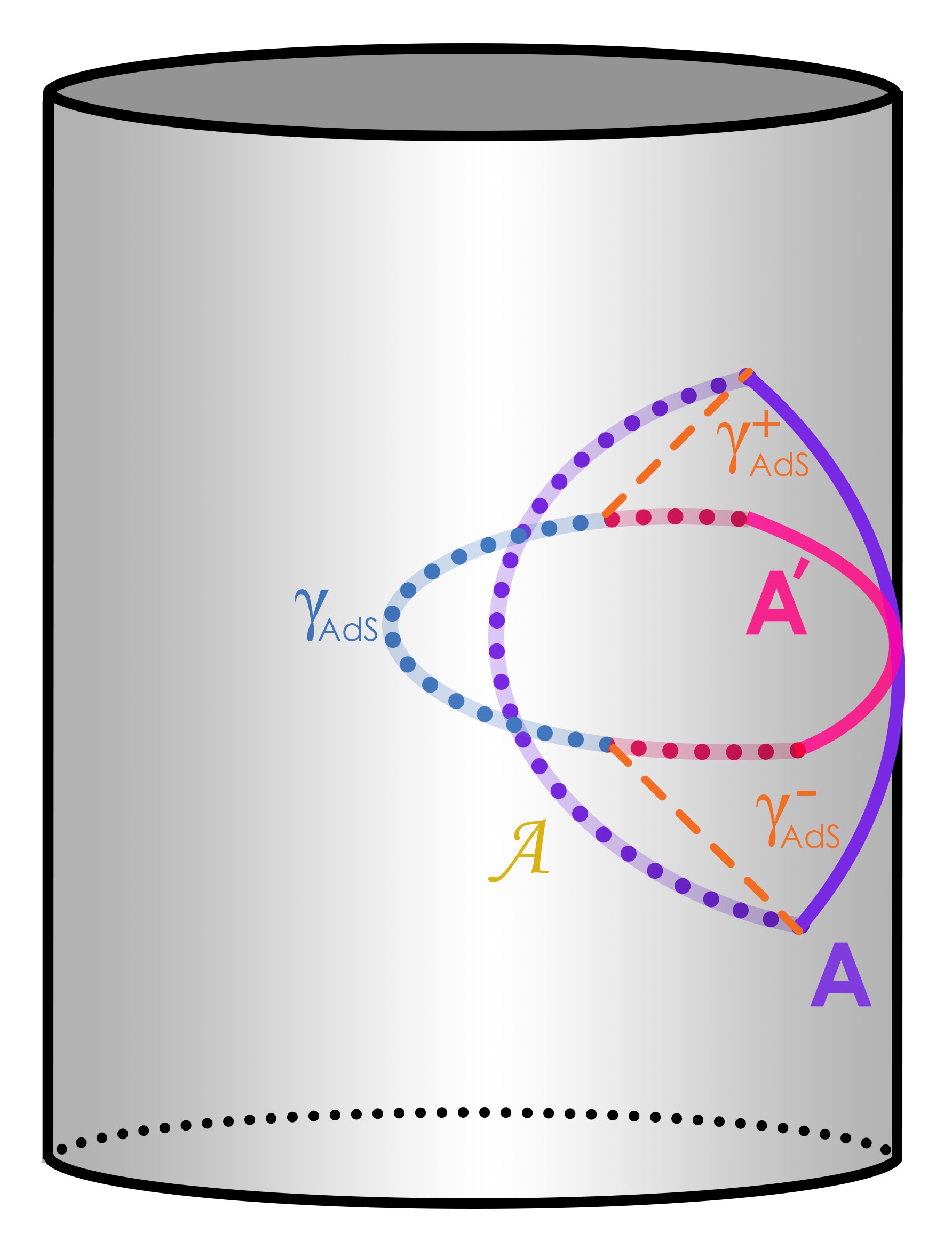
Figure 1: Curve $\mathbf{A}$ is the boundary interval and $\mathcal{A}$ is the extremal curve given by the RT prescription. $\mathbf{A^{\prime}}$ is the new interval and $\gamma_{AdS}$ is the new extremal curve. $\gamma^{\pm}_{AdS}$ connects end points of $\mathbf{A}$ to $\gamma_{AdS}$.

Starting from geodesic equations of metric (3.1), we look for null geodesics that connects $(u=-l_{u}/2,\phi=-l_{\phi}/2)$ and $(u=l_{u}/2,\phi=l_{\phi}/2)$ at $r=\infty$ to the new curve (3.3). Solving the geodesic equations with this conditions yields the following results:

• $\gamma^{-}_{AdS}$ is a null ray that connects $(u=-l_{u}/2,\phi=-l_{\phi}/2)$ to $\gamma_{AdS}$ and it is determined by equation

  $$u=-\dfrac{l_{u}}{2}+\dfrac{\beta_{-}}{r},\qquad\phi=-\dfrac{l_{\phi}}{2}+\dfrac{\alpha_{-}}{r},$$ (3.22)

  where $\alpha_{-}$ and $\beta_{-}$ are two constants determined by using the following equation

  $$\alpha_{-}^{2}+2\beta_{-}-\dfrac{\beta_{-}^{2}}{\ell^{2}}=0.$$ (3.23)

• $\gamma^{+}_{AdS}$ is a null geodesic which connects $(u=l_{u}/2,\phi=l_{\phi}/2)$ to $\gamma_{AdS}$. It is given by

  $$u=\dfrac{l_{u}}{2}+\dfrac{\beta_{+}}{r},\qquad\phi=\dfrac{l_{\phi}}{2}+\dfrac{\alpha_{+}}{r},$$ (3.24)

  where $\alpha_{+}$ and $\beta_{+}$ are two constants, satisfy the following equation

  $$\alpha_{+}^{2}+2\beta_{+}-\dfrac{\beta_{+}^{2}}{\ell^{2}}=0.$$ (3.25)

Thus, instead of a unique curve, we spot a bunch of curves for $\gamma^{\pm}_{AdS}$. The interesting point is that $\lambda^{\mu}$ is tangent to all of these curves. To determine unique null rays emanating from the end points of the boundary interval, we demand that these curves intersects some cutoff points. Precisely, we demand that $\gamma^{+}_{AdS}$ passes through $\left(r=\dfrac{1}{\epsilon_{+}},u=\dfrac{l_{u}}{2}-\epsilon_{u},\phi=\dfrac{l_{\phi}}{2}-\epsilon_{\phi}\right)$ and $\gamma^{-}_{AdS}$ crosses $\left(u=-\dfrac{l_{u}}{2}+\epsilon_{u},\phi=\dfrac{-l_{\phi}}{2}\epsilon_{\phi}\right)$ at $r=\dfrac{1}{\epsilon_{-}}$, where $\epsilon_{u}$, $\epsilon_{\phi}$, and $\epsilon_{\pm}$ are infinitesimal positive constants and $\epsilon_{u}/\epsilon_{\phi}$ is finite. With these conditions, we find that $\beta_{\pm}=\dfrac{\epsilon_{u}}{\epsilon_{\phi}}\alpha_{\pm}$, and there are two sets of solutions for $\alpha_{\pm}$:

$$\begin{cases}&\alpha_{+}=\alpha_{-}=0\\ &\,\,\,\,\,\,\,\,\text{or}\\ &\alpha_{+}=\alpha_{-}=-\dfrac{\dfrac{2\epsilon_{u}}{\epsilon_{\phi}}}{1-\dfrac{\epsilon_{u}^{2}}{\ell^{2}\epsilon_{\phi}^{2}}}.\end{cases}$$ (3.26)

For the second case, after taking the flat-space limit, one can deduce that $\epsilon_{\pm}<0$, which is opposed to our earlier assumption. Thus, we need to choose $\alpha_{+}=\alpha_{-}=\beta_{+}=\beta_{-}=0$, the flat-space limit of which results in $\gamma_{\pm}$ of Jiang:2017ecm,[0]Ref. [13].

3.4 Our proposal for calculation of holographic BMSFT entanglement entropy

In the previous subsections, we proposed a holographic method for the calculation of BMSFT entanglement entropy, which does not use the Rindler method and takes a flat-space limit from the calculations of the AdS/CFT correspondence. In this subsection, we summarize our method and provide a generic recipe:

• In the first step we need to find an asymptotically AdS spacetime that its flat-space limit is well-defined and results in our asymptotically flat metric. For this purpose, we need to write our metric and the interval at null infinity in the BMS gauge.

• For the asymptotically AdS metric and its corresponding interval, we can use RT prescription or its generalizations to gain an extremal curve in bulk, the length which is proportional to the entanglement entropy of the interval.

• The bulk modular flow is a Killing vector that is vanishing on the extremal curve. So, our next step is finding bulk modular flow by using the extremal curve of the asymptotically AdS case.

• Using the bulk modular flow, we look for a new Killing vector which is normal to it, and their norms satisfy (3.2). This new vector has a well-defined flat-space limit, which is the bulk modular flow of the corresponding asymptotically flat spacetimes.

• The points in bulk in which the components of the new vector are vanishing construct a new extremal curve in the asymptotically AdS spacetime. The flat-space limit of this new curve is well defined and yields a curve in the asymptotically flat spacetime that $\gamma$ is a part of it.

• In the next step, we look for the null geodesics that start from end points of the interval and intersect our new extremal curve. The flat-space limit of these curves results in $\gamma_{\pm}$. However, instead of a unique curve, we encounter a bunch of curves with this property. We remove this ambiguity by demanding that the desired null curve must pass through another point in the spacetime, which we call the cutoff point.

• Knowing $\gamma$ and $\gamma_{\pm}$, we can calculate the length of $\gamma$, which is proportional to the entanglement entropy of the interval in BMSFT.

4 Conclusion

We introduced new curves in the three-dimensional asymptotically AdS spacetimes whose flat-space limit yields the extremal curves in the asymptotically flat spacetimes. These curves can be used for the holographic calculation of the dual BMSFT entanglement entropy. In our proposal, a new vector field, which is normal to the bulk modular flow of the corresponding CFT interval, plays an important role. In fact, instead of the BMSFT interval, we considered a similar CFT interval, and using the RT proposal, we found the extremal curve and also the bulk modular flow in the asymptotically AdS spacetime. Then, using the Killing equation and also normality and norm conditions, we found a new vector field. The points in the spacetime in which this new vector field is vanishing construct a curve with a well-defined flat-space limit. We also have proposed two null rays with a well-defined flat-space limit in the asymptotically AdS spacetime, which connects end points of the interval to the new extremal curve. The flat-space limit of these curves together provides a holographic description for the BMSFT entanglement entropy proposed previously in Jiang:2017ecm,[0]Ref. [13].

We proposed our method as an alternative method for finding the holographic entanglement entropy of BMSFTs, which does not need to use Rindler transformation. However, in the first part of the current paper, we developed our method by arguing that the new RT-like extremal curves are those curves that map to the inner horizon of BTZ black holes. Using this fact, we could find two main formulas of this paper (3.2). In this view, the importance of the inner horizon in this work is to help us find (3.2). As a result, the connection with the inner horizon is absent in the steps which we propose as a recipe to calculate the holographic entanglement entropy of BMSFTs. Moreover, in the context of the current paper, before taking the flat-space limit, these new extremal curves are not crucial for extracting new information about the holographic entanglement entropy of CFT intervals. Thus, one can escape from the unclear points which arise by extrapolating the known methods in the AdS/CFT correspondence to the inner horizons.

Our method can be generalized to the higher dimensions. One of the future directions is applying it to find the entanglement entropy of three-dimensional BMSFTs which are dual to the four-dimensional asymptotically flat spacetimes. To do so, we need to overcome some circumstances. In general, modular flows can only be identified with geometric flows generated by Killing vectors when the modular Hamiltonian is local. In three dimensions that any arbitrary interval in the boundary CFT is a line segment, the modular Hamiltonian is local. In higher dimensions, only spherical entangling regions will generate local modular Hamiltonians, so the interpretation of this modular Hamiltonian as generating a geometric flow, which is along the direction of a Killing vector, breaks down. Thus, the RT surface can no longer be considered as a Killing horizon.

Moreover, this method can be used to relate the first law of entanglement entropy in the boundary theory to the linearized equation of motion of the bulk theory Lashkari:2013koa,eom,[0]Ref. [27, 28]. In the context of flat/BMSFT, this relation has been studied earlier in Godet:2019wje,Fareghbal:2019czx,[0]Ref. [29, 30] (see also more recent papers Apolo:2020bld,Apolo:2020qjm,[0]Ref. [31, 32]). The main advantage of our method is that one can study this problem by taking the flat-space limit from the known results in the AdS/CFT. For example, the extremal curves related to perturbed geometry in the asymptotically flat spacetime can be found by taking the flat-space limit from the extremal curves in the asymptotically AdS spacetime. We plan to study this problem in our future works.

Acknowledgements

We would like to thank Yousef Izadi for his comments on the manuscript. We are also grateful to Daniel Grumiller and Masoud Gharahi Ghahi for useful discussions. M. H. is grateful for the hospitality of TU Wien where the last part of the current paper was done. We would also like to thank the referee for his/her useful comments. This work is supported by Iran National Science Foundation, Project No. 97017212.

Appendix A Rindler transformation

We are looking for a Rindler transformation which changes

$$ds^{2}=-\dfrac{r^{2}}{\ell^{2}}du^{2}-2dudr+r^{2}d\phi^{2},$$ (A.1)

to a BTZ black hole written in the BMS coordinate,

$$ds^{2}=\left(-\frac{\tilde{r}^{2}}{\ell^{2}}+\mathcal{\tilde{M}}\right)d\tilde{u}^{2}-2d\tilde{u}d\tilde{r}+2\mathcal{\tilde{N}}d\tilde{u}d\tilde{\phi}+\tilde{r}^{2}d\tilde{\phi}^{2},$$ (A.2)

where $\mathcal{\tilde{M}}$ and $\mathcal{\tilde{N}}$ are constants and are given in terms of the BTZ inner and outer horizons $\tilde{r}_{\pm}$ as

$$\mathcal{\tilde{M}}=\dfrac{\tilde{r}_{+}^{2}+\tilde{r}_{-}^{2}}{\ell^{2}},\qquad\mathcal{\tilde{N}}=\dfrac{\tilde{r}_{+}\tilde{r}_{-}}{\ell}.$$ (A.3)

To use the transformations which were introduced in the literature, we use (2.2) and (3.1) to change (A.1) to a Poincaré coordinate,

$$ds^{2}=\dfrac{\ell^{2}}{z^{2}}\left(dz^{2}-dt^{2}+dx^{2}\right).$$ (A.4)

Then, using the transformation

$$\rho=\dfrac{1}{2z^{2}},\quad U=x-t,\quad V=t+x,$$ (A.5)

we change (A.4) to

$$ds^{2}=\ell^{2}\left(\dfrac{d\rho^{2}}{4\rho^{2}}+2\rho dUdV\right).$$ (A.6)

The corresponding Rindler transformation is given by (7.2) of Jiang:2017ecm,[0]Ref. [13] as

$$T_{\tilde{U}}\tilde{U}= \frac{1}{4}\log\Big{[}\frac{(1+\rho(2U+l_{U})V)^{2}-\rho^{2}l_{V}^{2}(l_{U}/2+U)^{2}}{(1+\rho(2U-l_{U})V)^{2}-\rho^{2}l_{V}^{2}(l_{U}/2-U)^{2}}\Big{]}\,,$$ (A.7)

$$T_{\tilde{V}}\tilde{V}= \frac{1}{4}\log\Big{[}\frac{(1+\rho(2V+l_{V})U)^{2}-\rho^{2}l_{U}^{2}(l_{V}/2+V)^{2}}{(1+\rho(2V-l_{V})U)^{2}-\rho^{2}l_{U}^{2}(l_{V}/2-V)^{2}}\Big{]}\,,$$ (A.8)

$$\frac{\tilde{\rho}}{T_{\tilde{U}}T_{\tilde{V}}}= \frac{\rho^{2}\left(l_{U}^{2}\left(l_{V}^{2}-4V^{2}\right)-4U^{2}l_{V}^{2}\right)+4(2\rho UV+1)^{2}}{4\rho l_{U}l_{V}}\,,$$ (A.9)

and transforms (A.6) to

$$ds^{2} =\ell^{2}\left(T_{\tilde{U}}^{2}\,d\tilde{U}^{2}+2\tilde{\rho}\,d\tilde{U}d\tilde{V}+T_{\tilde{V}}^{2}d\tilde{V}^{2}+\frac{d\tilde{\rho}^{2}}{4(\tilde{\rho}^{2}-T_{\tilde{U}}^{2}T_{\tilde{V}}^{2})}\right)\,.$$ (A.10)

The final part of the transformation is given by

$$\tilde{U}= \frac{\tanh^{-1}\left(\frac{2\tilde{r}}{T_{\tilde{V}}-T_{\tilde{U}}}\right)-\tanh^{-1}\left(\frac{2\tilde{r}}{T_{\tilde{V}}+T_{\tilde{U}}}\right)}{2T_{\tilde{U}}}+\frac{\ell\tilde{\phi}+\tilde{u}}{2\ell^{2}}\,,$$ (A.11)

$$\tilde{V}= \frac{\tanh^{-1}\left(\frac{2\tilde{r}}{T_{\tilde{V}}-T_{\tilde{U}}}\right)+\tanh^{-1}\left(\frac{2\tilde{r}}{T_{\tilde{V}}+T_{\tilde{U}}}\right)}{2T_{\tilde{V}}}+\frac{\ell\tilde{\phi}-\tilde{u}}{2\ell^{2}}\,,$$ (A.12)

$$\tilde{\rho}= \frac{1}{2}\left(4\tilde{r}^{2}-T_{\tilde{V}}^{2}-T_{\tilde{U}}^{2}\right)\,,$$ (A.13)

which transforms (A.10) to (A.2), and we have

$$T_{\tilde{U}}=\tilde{r}_{+}+\tilde{r}_{-},\qquad T_{\tilde{V}}=\tilde{r}_{+}-\tilde{r}_{-}.$$ (A.14)

Appendix B Holographic entanglement entropy of BMSFT dual to global Minkowski

Let us consider an interval in BMSFT₂ dual to the three-dimensional global Minkowski spacetime given by the following metric:

$$ds^{2}=-d\hat{u}^{2}-2d\hat{u}d\hat{r}+\hat{r}^{2}d\hat{\phi}^{2}.$$ (B.1)

The interval is determined by

$$\hat{u}=\dfrac{L_{u}\sin\hat{\phi}}{2\sin\dfrac{L_{\phi}}{2}},$$ (B.2)

and end points of it are at $(\hat{u}=-L_{u}/2,\hat{\phi}=-L_{\phi}/2)$ and $(\hat{u}=+L_{u}/2,\hat{\phi}=+L_{\phi}/2)$.

The metric (B.1) is given by taking the flat-space limit from the global AdS written in the BMS gauge,

$$ds^{2}=-\left(1+\dfrac{\hat{r}^{2}}{\ell^{2}}\right)d\hat{u}^{2}-2d\hat{u}d\hat{r}+\hat{r}^{2}d\hat{\phi}^{2}.$$ (B.3)

To find the holographic entanglement of the interval (B.2) in BMSFT, we start with the same interval in the dual CFT₂ of (B.3). The bulk modular flow, $\xi^{\mu}$, and the new vector $\lambda^{\mu}$ are given by using the following transformation from (3.1) and (3.2):

$$r=\frac{1}{2}\left(\ell\sin\dfrac{\hat{u}}{\ell}+\hat{r}\cos\dfrac{\hat{u}}{\ell}+\hat{r}\cos\hat{\phi}\right),$$

$$\phi=\dfrac{\hat{r}\sin\hat{\phi}}{r},$$

$$u=\dfrac{\ell}{r}\left(\ell-\ell\cos\dfrac{\hat{u}}{\ell}+\hat{r}\sin\dfrac{\hat{u}}{\ell}\right).$$ (B.4)

The transformation (B) determines $l_{\phi}$ and $l_{u}$ in terms of $L_{\phi}$ and $L_{u}$,

$$l_{u}=\frac{4\ell\sin\left(\frac{L_{u}}{2\ell}\right)}{\cos\left(\frac{L_{u}}{2\ell}\right)+\cos\left(\frac{L_{\phi}}{2}\right)},\qquad l_{\phi}=\frac{4\sin\left(\frac{L_{\phi}}{2}\right)}{\cos\left(\frac{L_{u}}{2\ell}\right)+\cos\left(\frac{L_{\phi}}{2}\right)},$$ (B.5)

and gives $\xi^{\mu}$ and $\lambda^{\mu}$ of the global AdS as follows:

$$\xi=\frac{4\pi\left(\cos\left(\hat{\phi}\right)\sin\left(\frac{L_{\phi}}{2}\right)\cos\left(\frac{L_{u}}{2\ell}\right)\left(\ell\cos\left(\frac{\hat{u}}{\ell}\right)-\hat{r}\sin\left(\frac{\hat{u}}{\ell}\right)\right)+\sin\left(\hat{\phi}\right)\cos\left(\frac{L_{\phi}}{2}\right)\sin\left(\frac{L_{u}}{2\ell}\right)\left(\hat{r}\cos\left(\frac{\hat{u}}{\ell}\right)+\ell\sin\left(\frac{\hat{u}}{\ell}\right)\right)\right)}{\cos\left(L_{\phi}\right)-\cos\left(\frac{L_{u}}{\ell}\right)}\partial_{\hat{r}}+$$

$$\frac{2\pi\ell\left(-2\cos\left(\hat{\phi}\right)\sin\left(\frac{L_{\phi}}{2}\right)\cos\left(\frac{\hat{u}}{\ell}\right)\cos\left(\frac{L_{u}}{2\ell}\right)-2\sin\left(\hat{\phi}\right)\cos\left(\frac{L_{\phi}}{2}\right)\sin\left(\frac{\hat{u}}{\ell}\right)\sin\left(\frac{L_{u}}{2\ell}\right)+\sin\left(L_{\phi}\right)\right)}{\cos\left(L_{\phi}\right)-\cos\left(\frac{L_{u}}{\ell}\right)}\partial_{\hat{u}}+$$ (B.6)

$$\frac{2\pi\left(2\cos\left(\hat{\phi}\right)\cos\left(\frac{L_{\phi}}{2}\right)\sin\left(\frac{L_{u}}{2\ell}\right)\left(\hat{r}\cos\left(\frac{\hat{u}}{\ell}\right)+\ell\sin\left(\frac{\hat{u}}{\ell}\right)\right)+2\sin\left(\hat{\phi}\right)\sin\left(\frac{L_{\phi}}{2}\right)\cos\left(\frac{L_{u}}{2\ell}\right)\left(\hat{r}\sin\left(\frac{\hat{u}}{\ell}\right)-\ell\cos\left(\frac{\hat{u}}{\ell}\right)\right)-\hat{r}\sin\left(\frac{L_{u}}{\ell}\right)\right)}{\hat{r}\left(\cos\left(L_{\phi}\right)-\cos\left(\frac{L_{u}}{\ell}\right)\right)}\partial_{\hat{\phi}},$$

$$\lambda=-\frac{4\pi\left(\cos\left(\hat{\phi}\right)\cos\left(\frac{L_{\phi}}{2}\right)\sin\left(\frac{L_{u}}{2\ell}\right)\left(\ell\cos\left(\frac{\hat{u}}{\ell}\right)-\hat{r}\sin\left(\frac{\hat{u}}{\ell}\right)\right)+\sin\left(\hat{\phi}\right)\sin\left(\frac{L_{\phi}}{2}\right)\cos\left(\frac{L_{u}}{2\ell}\right)\left(\hat{r}\cos\left(\frac{\hat{u}}{\ell}\right)+\ell\sin\left(\frac{\hat{u}}{\ell}\right)\right)\right)}{\cos\left(L_{\phi}\right)-\cos\left(\frac{L_{u}}{\ell}\right)}\partial_{\hat{r}}+$$

$$\frac{2\pi\ell\left(2\cos\left(\hat{\phi}\right)\cos\left(\frac{L_{\phi}}{2}\right)\cos\left(\frac{\hat{u}}{\ell}\right)\sin\left(\frac{L_{u}}{2\ell}\right)+2\sin\left(\hat{\phi}\right)\sin\left(\frac{L_{\phi}}{2}\right)\sin\left(\frac{\hat{u}}{\ell}\right)\cos\left(\frac{L_{u}}{2\ell}\right)-\sin\left(\frac{L_{u}}{\ell}\right)\right)}{\cos\left(L_{\phi}\right)-\cos\left(\frac{L_{u}}{\ell}\right)}\partial_{\hat{u}}+$$ (B.7)

$$\frac{2\pi\left(-2\cos\left(\hat{\phi}\right)\sin\left(\frac{L_{\phi}}{2}\right)\cos\left(\frac{L_{u}}{2\ell}\right)\left(\hat{r}\cos\left(\frac{\hat{u}}{\ell}\right)+\ell\sin\left(\frac{\hat{u}}{\ell}\right)\right)+2\sin\left(\hat{\phi}\right)\cos\left(\frac{L_{\phi}}{2}\right)\sin\left(\frac{L_{u}}{2\ell}\right)\left(\ell\cos\left(\frac{\hat{u}}{\ell}\right)-\hat{r}\sin\left(\frac{\hat{u}}{\ell}\right)\right)+\hat{r}\sin\left(L_{\phi}\right)\right)}{\hat{r}\left(\cos\left(L_{\phi}\right)-\cos\left(\frac{L_{u}}{\ell}\right)\right)}\partial_{\hat{\phi}}.$$

It is clear that these two vector fields transform to each other by using the transformation

$$L_{u}\Rightarrow\ell\,L_{\phi},\qquad L_{\phi} \Rightarrow\dfrac{L_{u}}{\ell}.$$ (B.8)

The rest of the calculation is straightforward, and one can find $\gamma_{AdS}$ and also $\gamma_{\pm}$ and take the flat-space limit from them to obtain $\gamma$ and $\gamma_{\pm}$ in the global Minkowski spacetime. The final results are the same as in Jiang:2017ecm,[0]Ref. [13].

References

- [1] A. Bagchi, “Correspondence between Asymptotically Flat Spacetimes and Nonrelativistic Conformal Field Theories,” Phys. Rev. Lett. 105, 171601 (2010). A. Bagchi, “The BMS/GCA correspondence,” arXiv:1006.3354 [hep-th].
- [2] A. Bagchi and R. Fareghbal, “BMS/GCA Redux: Towards Flatspace Holography from Non-Relativistic Symmetries,” JHEP 1210, 092 (2012) [arXiv:1203.5795 [hep-th]].
- [3] J. Levy-Leblond, Une nouvelle limite non-relativiste du group de Poincare, Ann. Inst. H. Poincare 3 (1965) 1.
- [4] C. Duval, G. W. Gibbons, P. A. Horvathy and P. M. Zhang, Carroll versus Newton and Galilei: two dual non-Einsteinian concepts of time, Class. Quant. Grav. 31 (2014) 085016 [1402.0657].
- [5] G. Barnich and G. Compere, “Classical central extension for asymptotic symmetries at null infinity in three spacetime dimensions,” Class. Quant. Grav. 24, F15 (2007) [gr-qc/0610130].
- [6] H. Bondi, M. G. van der Burg, and A. W. Metzner, “Gravitational waves in general relativity. 7. Waves from axisymmetric isolated systems,” Proc. Roy. Soc. Lond. A 269 (1962) 21. R. K. Sachs, “Gravitational waves in general relativity. 8. Waves in asymptotically flat space-times,” Proc. Roy. Soc. Lond. A 270 (1962) 103. R. K. Sachs, “Asymptotic symmetries in gravitational theory,” Phys. Rev. 128 (1962) 2851.
- [7] G. Barnich and C. Troessaert, “Symmetries of asymptotically flat 4 dimensional spacetimes at null infinity revisited,” arXiv:0909.2617 [gr-qc].
- [8] G. Barnich and C. Troessaert, “Aspects of the BMS/CFT correspondence,” JHEP 1005, 062 (2010) [arXiv:1001.1541 [hep-th]].
- [9] A. Ashtekar, J. Bicak and B. G. Schmidt, “Asymptotic structure of symmetry reduced general relativity,” Phys. Rev. D 55, 669 (1997) [gr-qc/9608042].
- [10] A. Bagchi, A. Mehra and P. Nandi, “Field Theories with Conformal Carrollian Symmetry,” JHEP 05 (2019), 108 doi:10.1007/JHEP05(2019)108 [arXiv:1901.10147 [hep-th]].
- [11] A. Bagchi, R. Basu, A. Mehra and P. Nandi, “Field Theories on Null Manifolds,” JHEP 02 (2020), 141 doi:10.1007/JHEP02(2020)141 [arXiv:1912.09388 [hep-th]].
- [12] A. Bagchi, R. Basu, D. Grumiller and M. Riegler, “Entanglement entropy in Galilean conformal field theories and flat holography,” Phys. Rev. Lett. 114, no. 11, 111602 (2015) doi:10.1103/PhysRevLett.114.111602 [arXiv:1410.4089 [hep-th]].
- [13] H. Jiang, W. Song and Q. Wen, “Entanglement Entropy in Flat Holography,” JHEP 1707, 142 (2017) doi:10.1007/JHEP07(2017)142 [arXiv:1706.07552 [hep-th]].
- [14] S. Ryu and T. Takayanagi, “Holographic derivation of entanglement entropy from AdS/CFT,” Phys. Rev. Lett. 96, 181602 (2006) doi:10.1103/PhysRevLett.96.181602 [hep-th/0603001].
- [15] H. Casini, M. Huerta and R. C. Myers, “Towards a derivation of holographic entanglement entropy,” JHEP 05, 036 (2011) doi:10.1007/JHEP05(2011)036 [arXiv:1102.0440 [hep-th]].
- [16] R. Fareghbal and A. Naseh, “Aspects of Flat/CCFT Correspondence,” Class. Quant. Grav. 32, 135013 (2015) doi:10.1088/0264-9381/32/13/135013 [arXiv:1408.6932 [hep-th]].
- [17] M. Riegler, “Flat space limit of higher-spin Cardy formula,” Phys. Rev. D 91, no.2, 024044 (2015) doi:10.1103/PhysRevD.91.024044 [arXiv:1408.6931 [hep-th]].
- [18] L. Cornalba and M. S. Costa, “A New cosmological scenario in string theory,” Phys. Rev. D 66, 066001 (2002) doi:10.1103/PhysRevD.66.066001 [hep-th/0203031].
- [19] L. Cornalba and M. S. Costa, “Time dependent orbifolds and string cosmology,” Fortsch. Phys. 52, 145 (2004) doi:10.1002/prop.200310123 [hep-th/0310099].
- [20] A. Bagchi, S. Detournay, R. Fareghbal and J. Simón, “Holography of 3D Flat Cosmological Horizons,” Phys. Rev. Lett. 110, no. 14, 141302 (2013) doi:10.1103/PhysRevLett.110.141302 [arXiv:1208.4372 [hep-th]].
- [21] G. Barnich, “Entropy of three-dimensional asymptotically flat cosmological solutions,” JHEP 1210, 095 (2012) doi:10.1007/JHEP10(2012)095 [arXiv:1208.4371 [hep-th]].
- [22] C. Holzhey, F. Larsen and F. Wilczek, “Geometric and renormalized entropy in conformal field theory,” Nucl. Phys. B 424, 443-467 (1994) doi:10.1016/0550-3213(94)90402-2 [arXiv:hep-th/9403108 [hep-th]].
- [23] P. Calabrese and J. L. Cardy, “Entanglement entropy and quantum field theory,” J. Stat. Mech. 0406, P06002 (2004) doi:10.1088/1742-5468/2004/06/P06002 [arXiv:hep-th/0405152 [hep-th]].
- [24] G. Barnich, A. Gomberoff and H. A. Gonzalez, “The Flat limit of three dimensional asymptotically anti-de Sitter spacetimes,” Phys. Rev. D 86, 024020 (2012) doi:10.1103/PhysRevD.86.024020 [arXiv:1204.3288 [gr-qc]].
- [25] Q. Wen, “Towards the generalized gravitational entropy for spacetimes with non-Lorentz invariant duals,” JHEP 01, 220 (2019) doi:10.1007/JHEP01(2019)220 [arXiv:1810.11756 [hep-th]].
- [26] Q. Wen, “Fine structure in holographic entanglement and entanglement contour,” Phys. Rev. D 98, no.10, 106004 (2018) doi:10.1103/PhysRevD.98.106004 [arXiv:1803.05552 [hep-th]].
- [27] N. Lashkari, M. B. McDermott and M. Van Raamsdonk, “Gravitational dynamics from entanglement ’thermodynamics’,” JHEP 1404, 195 (2014) doi:10.1007/JHEP04(2014)195 [arXiv:1308.3716 [hep-th]].
- [28] T. Faulkner, M. Guica, T. Hartman, R. C. Myers and M. Van Raamsdonk, “Gravitation from Entanglement in Holographic CFTs,” JHEP 1403, 051 (2014) doi:10.1007/JHEP03(2014)051 [arXiv:1312.7856 [hep-th]].
- [29] V. Godet and C. Marteau, “Gravitation in flat spacetime from entanglement,” JHEP 12, 057 (2019) doi:10.1007/JHEP12(2019)057 [arXiv:1908.02044 [hep-th]].
- [30] R. Fareghbal and M. Hakami Shalamzari, “First Law of Entanglement Entropy in Flat-Space Holography,” Phys. Rev. D 100, no.10, 106006 (2019) doi:10.1103/PhysRevD.100.106006 [arXiv:1908.02560 [hep-th]].
- [31] L. Apolo, H. Jiang, W. Song and Y. Zhong, “Swing surfaces and holographic entanglement beyond AdS/CFT,” [arXiv:2006.10740 [hep-th]].
- [32] L. Apolo, H. Jiang, W. Song and Y. Zhong, “Modular Hamiltonians in flat holography and (W)AdS/WCFT,” [arXiv:2006.10741 [hep-th]].