Searching for cosmological gravitational-wave backgrounds with third-generation detectors in the presence of an astrophysical foreground

Abstract

The stochastic cosmological gravitational-wave background (CGWB) provides a direct window to study early universe phenomena and fundamental physics. With the proposed third-generation ground-based gravitational wave detectors, Einstein Telescope (ET) and Cosmic Explorer (CE), we might be able to detect evidence of a CGWB. However, to dig out these prime signals would be a difficult quest as the dominance of the astrophysical foreground from compact-binary coalescence (CBC) will mask this CGWB. In this paper, we study a subtraction-noise projection method, making it possible to reduce the residuals left after subtraction of the astrophysical foreground of CBCs, greatly improving our chances to detect a cosmological background. We carried out our analysis based on simulations of ET and CE and using posterior sampling for the parameter estimation of binary black-hole mergers. We demonstrate the sensitivity improvement of stochastic gravitational-wave searches and conclude that the ultimate sensitivity of these searches will not be limited by residuals left when subtracting the estimated BBH foreground, but by the fraction of the astrophysical foreground that cannot be detected even with third-generation instruments, or possibly by other signals not included in our analysis. We also resolve previous misconceptions of residual noise in the context of Gaussian parameter estimation.

I Introduction

The accomplishment of detecting gravitational waves (GWs) from the mergers of compact binaries with neutron stars and black holes opened a new window to study astrophysical and cosmological phenomena of the Universe. The continuous improvement in the sensitivity and multi-detection of signals due to coalescence of a binary neutron star (BNS) and various binary black-hole (BBH) mergers during the first two observation runs of Advanced LIGO Asai et al. (2015) and Advanced Virgo Acernese et al. (2014) marks the beginning of a cosmic catalog of sources so far reaching out to distances of about 3 Gpc and only capturing a small fraction of all compact binaries in this volume Abbott et al. (2019a).

A major objective of modern cosmology is to detect early-universe GW signals, which are crucial to test current cosmological models and to further our understanding of the evolution of the Universe Abbott et al. (2009); Ade et al. (2018). The cosmic GW background (CGWB) is predicted to arise from fundamental processes in the early universe Caprini and Figueroa (2018); Christensen (2018). Among these are quantum vacuum fluctuations amplified by inflation Turner (1997); Easther et al. (2007); Guzzetti et al. (2016), phase transitions Kamionkowski et al. (1994); Kahniashvili et al. (2008); Caprini et al. (2009, 2016), and also cosmic strings are prominent for CGWB searches with ET and CE Vachaspati and Vilenkin (1985); Damour and Vilenkin (2005); Siemens et al. (2007); Ölmez et al. (2010). On the theoretical side, there is huge advancement to understand the concept and generation of these cosmological signals and on the observational and experimental side, to detect these signals with GW detectors is also in advancement and provides us with the capability to detect these signals in the future.

However, the detection of a CGWB is extremely challenging. Mission concepts that would make the detection of a primordial stochastic background probable, the space-borne detectors Big-Bang Observer (BBO) Crowder and Cornish (2005) and DECIGO Kawamura et al. (2006), still require substantial advances in laser-interferometer technology, and it is unknown when or if these experiments will become operational. Two ground-based, third-generation GW detectors have been proposed, Einstein Telescope (ET) Punturo et al. (2010) and Cosmic Explorer (CE) Reitze et al. (2019), which are expected to be operational by 2035 and potentially with the capacity to detect a CGWB. Primordial stochastic signals are predicted to lie well below instrument noise of all conceived future GW detectors. The stochastic searches with GW detectors follow the cross-correlation method betting on the assumption that fields of stochastic GWs produce correlations between detectors, while the instrument noises do not, or in a well-understood way with options to mitigate correlated noise, e.g., by Schumann resonances Thrane et al. (2013); Coughlin et al. (2016). Optimal cross-correlation filters can be employed to obtain the maximum signal-to-noise ratio (SNR) integrated over a band of frequencies and thus maximize chances to detect a CGWB Christensen (1992); Allen and Romano (1999). It is also possible to estimate parameters of stochastic backgrounds such as spectral slopes and possible anisotropies of the GW field Ballmer (2006); Romano (2019).

With the proposed third-generation GW detectors ET and CE, we will step into a new era of GW physics, and we will overcome the scarcity of GW sources, such that we will be able to detect binary signals up to high redshifts $z\geq 10$. Analyses of data from the first and second observation runs of LIGO and VIRGO constrain the local BBH merger rate to about 10 – 100 Gpc^-3y^-1 Abbott et al. (2019a). The BBH merger rate as a function of redshift is estimated from the star-formation rate Vangioni et al. (2015), distribution of time-delays between formation and merger Belczynski et al. (2002), and by normalizing to the local merger rate Vitale et al. (2019). It predicts about $10^{5}-10^{6}$ BBH mergers per year and a large fraction of them detectable with ET or CE. Since the correlation between detectors is predicted to be dominated by the astrophysical foreground of compact-binary coalescences (CBCs), detection of a cosmological background is strongly impeded and mitigation of the foreground is required.

As a first step, the foreground can be reduced by subtracting the estimated waveforms of all detected signals. Previous work has shown that a combination of unresolved sources, i.e., signals lying below the detection threshold, and residuals left in the data after subtraction can still limit the sensitivity of CGWB searches with future GW detector networks Regimbau et al. (2017); Sachdev et al. (2020). Both publications neglected the possibility to reduce subtraction residuals as proposed in earlier work for space-borne detectors Cutler and Harms (2006); Harms et al. (2008). Furthermore, a full-Bayesian analysis of primordial and astrophysical signals is expected to lower the impact of sub-threshold signals Smith and Thrane (2018). In this paper, we deal with the problem of reducing the subtraction residuals of the astrophysical foreground in third-generation detectors ET and CE, and for this goal we test the subtraction-noise projection method for BBHs Cutler and Harms (2006); Harms et al. (2008). As was pointed out in a recent publication Sachdev et al. (2020), the foreground of binary neutron stars (BNS) is expected to be more challenging to reduce, but we have no means yet to simulate this problem beyond what has already been done in previous work, as it requires an effective posterior sampler for parameter estimation in ET, which is a major challenge due to the length of BNS waveforms in ET (around a day), and it needs to account for the rotation of Earth during observation time.

The paper is organized as follows. Details of the simulation of the detector network and its astrophysical foreground are presented in section II. Section III reviews the geometrical interpretation of matched filtering, and provides an estimate of residual noise from an astrophysical foreground. In section IV, we explain the projection method that reduces residuals of the astrophysical foreground. The cross-correlation measurement between CE and ET is detailed in section V. Results of the foreground-mitigation procedure are discussed in section VI.

II Simulation Overview

The second-generation detectors Advanced LIGO and Advanced Virgo, after gradual updates, already observed several tens of binary-merger signals including the candidates of the last observing run Abbott et al. (2019a). There is still a huge spectrum of GW physics unexplored both in astrophysics and cosmology. In future, the main focus will be to exploit this vast spectrum. To progress in this direction, we need next-generation GW detectors with much better sensitivity than current GW detector. Two ground-based detectors have been proposed so far: the European Einstein Telescope and the US Cosmic Explorer Punturo et al. (2010); Abbott et al. (2017). Individually and as a detector network together with developed versions of current-generation detectors (including KAGRA Akutsu et al. (2019) and LIGO India Souradeep (2016)), these third-generation detectors have a rich science case covering topics in fundamental physics, cosmology, astrophysics, and nuclear physics 3Gs (2019); Maggiore et al. (2019). Their projected sensitivities are shown in figure 1.

ET: ET is a proposed European third-generation, underground GW observatory in the shape of an equilateral triangle with 10 km side length. ET will provide an improvement in sensitivity by a factor of 10 with respect to current GW detectors, extending the observation band down to about 3 Hz Hild et al. (2011). The Einstein Telescope will be placed underground to reduce the environmental noise coming from seismic and atmospheric fields. The infrastructure will host three interferometer pairs, each pair consisting of a low-frequency and a high-frequency interferometer forming a so-called xylophone configuration Hild et al. (2009).

CE: CE is a proposed US third-generation, surface GW observatory with the traditional L-shape and arm length of 40 km. Its design also foresees a sensitivity improvement by about a factor 10 compared to current GW detectors. The sensitivity model employed in this study corresponds to the first phase of CE development (CE1 in Reitze et al. (2019)). Its ultimate sensitivity target is about a factor 2 better than this.

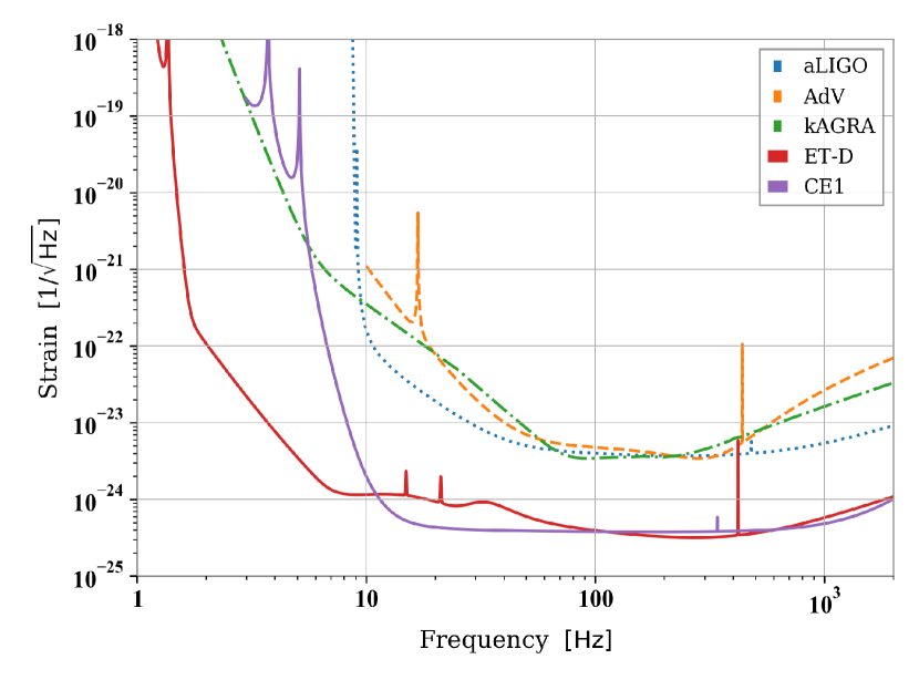
Figure 1: Design sensitivities of current and future GW detectors.

The basis of our simulation is the calculation of a 1.3-year-long stretch of GW data for ET (three individual data streams) and CE. The subtraction of best-fit waveforms is carried out in time domain, while the residual-noise projection is easiest to perform in the domain of the waveform model (frequency domain in our case) as explained in section IV. The projection requires Fisher matrices, which in turn require the derivatives of waveforms with respect to their parameters. We carry out the differentiation numerically so that in future, we can use this simulation also to study systematics related to waveform modeling without requiring analytic waveforms. Cross-spectral densities (CSDs) of time series between all four detectors are calculated after each of the following steps,

1. creation of time series only with instrument noise,

2. injection of GW signals in all four detectors (3 ET + 1 CE),

3. subtraction of best-fit waveforms,

4. residual-noise projection,

to demonstrate the impact of each step on the CSD. Finally, optimal filters are applied for an evaluation of the ultimate sensitivity of the network to a CGWB.

Whenever possible, our analysis uses functions of the Python parameter-estimation software package Bilby Ashton et al. (2019). The calculation of noise time series is done by built-in functions of Bilby using instrument noise models of ET and CE in the form of spectral densities. Also injection of GW signals in the data, and posterior sampling are done with Bilby. Subtraction of the best-fit waveforms is done using the injection algorithm with a change of the sign of the waveform. The projection of residual noise is mostly based on original code. The optimal filters used in the final step for the detection of a CGWB depend on the overlap-reduction function between detectors Christensen (1992); Allen and Romano (1999), which can be calculated straight-forwardly using antenna patterns provided by Bilby.

The astrophysical foreground is formed by the mergers of compact binaries with black holes and neutron stars. The lowest-mass members of these binaries, especially the binary neutron stars, take a special role (from today’s perspective) since it is still prohibitively expensive to simulate parameter estimation accurately for ET given that these signals can last for more than a day in the ET observation band and generally require high sampling frequencies to study the merger physics. A multi-band analysis of individual signals might provide a solution Adams et al. (2016); Vinciguerra et al. (2017), but there is no parameter-estimation package yet based on posterior sampling and implementing all required effects such as the impact of Earth’s rotation on the GW signal. For this reason, we chose to focus on BBH mergers in this paper. It allows us to use state-of-the-art parameter estimation software for posterior sampling.

However, even when focusing on BBH mergers, providing parameter estimations of $10^{5}-10^{6}$ signals by posterior sampling, which is an important new ingredient in this work compared to previous studies of the projection method, is computationally prohibitively expensive. As a way forward, we adopted the following scheme. Only for 100 BBH signals, posterior sampling is performed. The complete stretch of data is divided into 10000 segments of length 4096 s. In each of the segments, all 100 waveforms are injected with random time shifts so that the merger occurs in the respective time segment. In this way, phase relations between all signals are randomized and the CSD between detectors has the properties of a stochastic foreground. Its overall amplitude is stronger than it would be in a more realistic simulation since we deliberately chose highest-SNR members of the cosmological distribution to have the clearest demonstration of the effect of residual-noise projection. We employ a redshift independent power-law distribution for both intrinsic masses with a power law index $\alpha=-1.6$ Abbott et al. (2019b) constraining the individual masses to lie within the range $5\mathcal{M}_{\odot}\leq m_{2}<m_{1}\leq 60\mathcal{M}_{\odot}$. This leads to the sample of 100 BBH masses shown in figure 2.

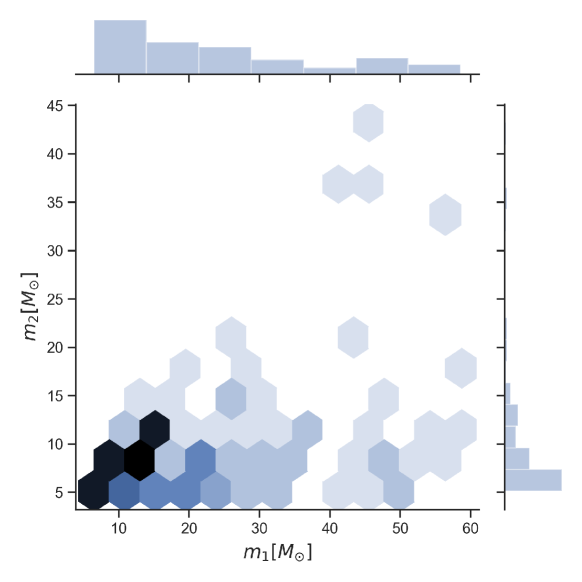
Figure 2: Mass range for individual BBH mass used in our study.

The sampled redshifts and total masses of the signals used in this paper are shown in figure 3 together with smoothed distributions derived from these samples (which explains why there is no low-mass bound of the mass distribution).

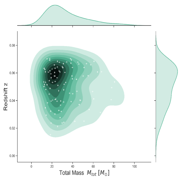
Figure 3: Distribution of total mass $M$ and redshift $z$ of the 100 BBH signals used in our analysis. High-SNR signals are chosen for clearest possible demonstration of the projection method to mitigate the astrophysical foreground.

III Matched filtering and the residual of an astrophysical foreground

The probability of two BBH signals to overlap in time in ET data is relatively high, but depends on details of the mass distribution Regimbau et al. (2017). Lower-mass signals last longer (up to a few minutes) and if present in greater number would lead to more frequent overlap. However, it is unlikely that the number of detectable BBH signals with 3G detectors will be impacted significantly by the presence of other signals, which is in contrast to the situation described for future space-borne GW detectors where the foreground acts as excess noise Danzmann et al. (2017); Cutler and Harms (2006). It is therefore enough to consider the impact of the astrophysical foreground on the correlation measurements between detectors, which is addressed by the subtraction-projection method discussed in the following using results from Cutler and Harms Cutler and Harms (2006).

The basis of the subtraction-projection method is the expansion of parameter errors or likelihood functions with respect to the inverse of the SNR of signals, which means that this approach works better for high-SNR signals. An important quantity is the Fisher matrix, whose components take the form

$$\begin{split}\Gamma_{\alpha\beta}&=<\partial_{\alpha}h(\vec{\lambda})|\partial_{\beta}h(\vec{\lambda})>\\ &=4\int_{0}^{\infty}df\frac{\Re(\partial_{\alpha}h(f)\partial_{\beta}h^{*}(f))}{S^{n}(f)},\end{split}$$ (1)

where $\vec{\lambda}$ is the vector of model parameters. The scalar product requires an estimate of the instrument-noise spectral density $S^{n}(f)$. We expressed the Fisher matrix as a scalar product $\langle\cdot|\cdot\rangle$ between derivatives of the waveform model with respect to model parameters $\partial_{\alpha}=\partial/\partial\lambda^{\alpha}$. The Fisher matrix can be interpreted as a metric on the curved template manifold defined by the waveform model $h(\vec{\lambda})$. The template manifold is a sub-manifold of the sampling space whose points describe realizations of detector data including instrument noise and signals not described by $h(\vec{\lambda})$.

If the best-fit waveform $\hat{h}$ maximizes the likelihood (standard parameter estimation maximizes the posterior that includes priors), i.e., if it minimizes $\langle s-\hat{h}|s-\hat{h}\rangle$, then for signals with sufficiently high SNR, $\hat{h}$ fulfills the following equation

$$\langle s-\hat{h}|\partial_{\alpha}\hat{h}\rangle=\langle n+(h-\hat{h})|\partial_{\alpha}\hat{h}\rangle=0$$ (2)

for all derivatives $\partial_{\alpha}$, with $n$ being the instrument noise and $h$ the GW signal contributing to the data $s$. The vanishing of the first scalar product in this equation means that the line in sampling space connecting the point $s$ with the best-fit waveform $\hat{h}$ is perpendicular to the template manifold, i.e., the best-fit waveform is obtained by determining the template on the manifold with minimal distance to $s$. The vanishing of the second scalar product means that the residual noise $\delta h=\hat{h}-h$ is equal to the component of the instrument noise tangent to the manifold at the point of the best-fit $\hat{h}$.

The scalar product can also be used to define the SNR of a signal:

$${\rm SNR}=\sqrt{\langle h|h\rangle}$$ (3)

The leading order term of a SNR^-1 expansion of the covariances of parameter-estimation errors $\delta\lambda^{\alpha}$ is given by

$$\overline{\delta\lambda^{\alpha}\delta\lambda^{\beta}}=\Gamma^{\alpha\beta},$$ (4)

where $\Gamma^{\alpha\beta}$ are the components of the inverse of the Fisher matrix. This relation is sometimes used to define an approximate Gaussian distribution of the likelihood function $\exp(-\Gamma_{\alpha\beta}\delta\lambda^{\alpha}\delta\lambda^{\beta}/2)$, and parameter-estimation errors can be drawn from this distribution to substitute a computationally costly posterior sampling Harms et al. (2008); Sachdev et al. (2020).

It is also possible to express the leading-order, parameter-estimation errors $\delta\lambda^{\alpha}$ in terms of a specific instrumental-noise realization $n$ as:

$$\delta\lambda^{\alpha}\equiv\hat{\lambda}^{\alpha}-\lambda^{\alpha}\approx\Gamma^{\alpha\beta}<n|\partial_{\beta}\hat{h}>.$$ (5)

Here, $\hat{\lambda}^{\alpha}$ are the parameter estimates determining the best-fit waveform $\hat{h}$. By using equation (4), we can calculate the norm-squared of the average subtraction residuals

$$\overline{<\delta h|\delta h>}=<\partial_{\alpha}\hat{h}|\partial_{\beta}\hat{h}>\overline{\delta\lambda^{\alpha}\delta\lambda^{\beta}}=\Gamma_{\alpha\beta}\Gamma^{\alpha\beta}=N_{p},$$ (6)

where $N_{p}$ is the total number of parameters going into the waveform model $h$. Together with equation (3) it tells us that in average, the amplitude of a signal after subtraction of its best-fit waveform is reduced by $\delta h/h\sim N_{p}^{1/2}/\rm SNR$, which also means that the residual is independent of the SNR of the signal (again, in the approximation of large SNR).

With the future GW detectors ET and CE we will be able to detect almost all the BBHs emitting within their observation bands, and the entire astrophysical foreground coming from $N_{S}$ sources is

$$H(t)=\sum_{k=1}^{N_{\rm S}}h^{k}(t).$$ (7)

With each BBH signal $h^{k}(t)$ being described by $N_{p}$ parameters, the parameter space of the complete astrophysical foreground has dimension $N_{p}\times N_{S}$. Therefore the norm-squared of the residual of this foreground is

$$\overline{<\delta H|\delta H>}=N_{p}\times N_{S}.$$ (8)

It is easy to show that in average

$$\delta H/H\approx\delta h/h,$$ (9)

which means that the fractional reduction of the amplitude of a single BBH is about the same of the entire astrophysical foreground assuming that (almost) all signals can be detected with sufficiently high SNR.

IV Projecting out the residual noise

The results of section III form the basis of the residual-noise projection, which we discuss in the following. As shown in equation (2), the residual noise is tangent to the waveform manifold. The strategy of the projection method is to apply a projection operator to the residual data $r=s-\hat{h}$ removing all of its components lying in the manifold’s tangent space at the best-fit waveform. This projection needs to be done for all the signals in the data. The projection operator can be written

$$P\equiv 1-\Gamma^{\alpha\beta}|\partial_{\alpha}\hat{h}><\partial_{\beta}\hat{h}|.$$ (10)

When applying the projection to the residual data of a detector $i$, one obtains

$$P[r_{i}](t)=r_{i}(t)-\Gamma_{i}^{\alpha\beta}\langle\partial_{\beta}\hat{h}_{i}|r_{i}\rangle\partial_{\alpha}\hat{h}_{i}(t),$$ (11)

which we wrote here for the time domain, but it can also be applied in Fourier domain. The residual $P[r_{i}]$ after projection corresponds to the instrument noise perpendicular to the template manifold plus a potential component of the true signal $h_{i}$ that does not lie in the tangent space of the best-fit $\hat{h}_{i}$. This residual of the signal is non-vanishing only for curved manifolds and is suppressed by SNR^-2 relative to the original signal. Comparing with equation (2), it seems that the projection operator should not have any effect on the residual data $r_{i}=s_{i}-\hat{h}_{i}$ since the vector $|r_{i}\rangle$ is normal to the tangent space of the template manifold at the best-fit. However, this is not necessarily correct for various reasons.

First, the maximum-likelihood parameter estimates $\hat{\lambda}^{\alpha}$ are obtained using data from all detectors in the network. These parameter values determine the best-fit waveforms $\hat{h}_{i}=h_{i}(\hat{\lambda}^{\alpha})$ of each detector $i$ in the network. These waveforms however are not the results of a normal projection of data vectors $|s_{i}\rangle$ onto the respective template manifolds. This would only be the case if maximum-likelihood estimates $\hat{\lambda}^{\alpha}_{i}$ are calculated for each detector separately. This means that subtracting $h_{i}(\hat{\lambda}^{\alpha})$ from the data of all detectors leaves residuals in the tangent spaces, which can be projected out. This also means that one needs to distinguish between the Fisher matrices $\Gamma_{i,\alpha\beta}(\hat{\lambda}_{i}^{\mu})$ and $\Gamma_{i,\alpha\beta}(\hat{\lambda}^{\mu})$, where the latter is obtained using the parameter estimates from a coherent network analysis.

Let us consider the case where the maximum-likelihood estimations are done for each detector separately producing different best-fit parameters $\hat{\lambda}^{\alpha}_{i}$ for each detector $i$. Then, subtracting $\hat{h}_{i}=h_{i}(\hat{\lambda}^{\alpha}_{i})$ for all signals in the data reduces the astrophysical foreground by 1/SNR² instead of 1/SNR. One might wonder where the subtraction residuals at order 1/SNR are, since clearly the misfit $\delta h_{i}$ is still only suppressed by $1/$SNR compared to the true signal $h_{i}(\lambda_{0}^{\alpha})$. Here, the important point is that when subtracting a signal, the residual $\delta h_{i}$ is already exactly canceled by the component $n_{\parallel}$ of the instrument noise that lies in the tangent space, which can be understood from equation (2) when using $n=n_{\perp}+n_{\parallel}$ and therefore $r=n_{\perp}$ plus residual noise from the astrophysical foreground suppressed by $1/$SNR² and higher.

Another reason why best-fit residuals can be in tangent spaces of a template manifold, even if the best-fits are calculated for each detector individually, is that they are typically not the result of a likelihood maximization, but of a maximization of the posterior distribution, which depends on priors. In this case, the residual $\delta h$ does not fulfill equation (2), and residuals in tangent spaces remain to be projected out.

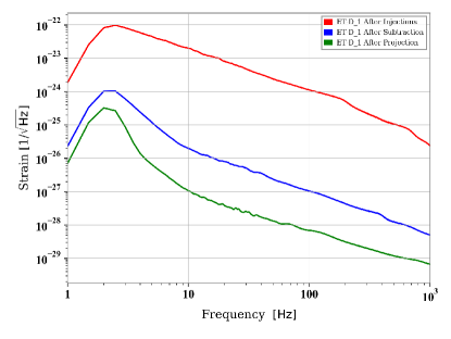
Figure 4: Simulated astrophysical foreground, subtraction residuals, and residual spectrum after projection for ET without instrument noise (except for the max-posterior parameter estimation).

Finally, technical choices of a simulation can lead to additional residuals in tangent spaces. Often, parameter estimation by posterior sampling is computationally too expensive for studies with a large population of signals. In this case, past work made use of equation (4) to define a Gaussian error distribution, from which parameter errors are drawn and added to the true signal parameters to obtain the maximum-likelihood parameters Harms et al. (2008); Sachdev et al. (2020). The issue here is that the parameter errors are not consistent with a specific realization of the instrument noise. The best-fit waveforms obtained in this way would not maximize the likelihood, and this leads to excess residual noise in tangent spaces, which is projected out Harms et al. (2008). This artifact can be avoided by using equation (5) to obtain parameter errors, which is still under the assumption of a Gaussian likelihood, but at least consistent with a specific noise realization.

As a first demonstration, we show the root power-spectral density of the astrophysical foreground averaged over 1.3 years, its subtraction residual, and the spectrum after projection in figure 4 without instrument noise for an ET detector. For this plot, time series were simulated without instrument noise just to demonstrate the full potential of the projection method. The posterior sampling was of course done including instrument noise, and included data from CE and the full ET triangle. The simulated astrophysical foreground is artificially enhanced to make sure that all signals have sufficiently high SNR to be able to neglect residuals at order 1/SNR². Furthermore, one needs to consider the possibility that some low-SNR signals are not detected by ET, which gives rise to additional contributions to residual noise that we do not consider in this study (see instead Regimbau et al. (2017); Sachdev et al. (2020)). It is interesting to observe that the spectra change their shape after applying the subtraction and projection, for which we cannot provide an explanation since our equations only predict residuals integrated over all frequencies.

V Stochastic background and Detection

The fractional energy-density spectrum of an isotropic stochastic background is defined as

$$\Omega_{GW}\left(f\right)~{}=~{}\frac{1}{\rho_{\rm c}}\cdot\frac{{\rm d}\rho_{\rm GW}}{{\rm d}\ln f},$$ (12)

where $\rho_{\rm c}~{}=~{}3H_{0}^{2}c^{2}/\left(8\pi G\right)$ is the critical energy density required for a flat universe, $H_{0}$ is the Hubble constant ($H_{0}=67.9\,\rm km\,s^{-1}Mpc^{-1}$ Ade et al. (2016)) and ${\rm d}\rho_{\rm GW}$ is the energy density of GWs contained in the frequency band $f$ to $f+{\rm d}f$ Allen and Romano (1999). The current limit on the gravitational-wave energy density spectrum is $\Omega_{\rm GW}<4.8\times 10^{-8}$ with $95\%$ confidence, in the band 20–100 Hz Abbott et al. (2019). In this work, we simulate searches optimized for an unpolarized, isotropic, stationary and Gaussian stochastic background. In reality, stochastic signals do not necessarily have these properties Allen and Romano (1999) except for stationarity, which is simply a consequence of short observation time compared to time scales characteristic for the evolution of GW distributions.

V.1 Cross-Correlation between Detectors

Cross-correlating the output of two or more GW detectors is the optimal strategy to detect a Gaussian, stationary stochastic GW background Christensen (1992); Allen and Romano (1999). Since we prefer to work in frequency domain, the cross-correlation is expressed as cross power-spectral density (CPSD) $C_{ij}(f)$ between two detectors $i,\,j$. We briefly review the steps to calculate the contribution of an isotropic, stochastic GW background to $C_{ij}(f)$ and how to calculate the statistical error due to instrument noise.

A stochastic GW background can be described as a plane-wave expansion of a metric perturbation

$$\begin{split}h_{\mu\nu}&(\vec{x},t)=\\ &\sum\limits_{A=+,\times}\int\limits_{s^{2}}{\rm d}\hat{\Omega}\int\limits_{-\infty}^{\infty}{\rm d}f\,h_{A}(f,\hat{\Omega}){\rm e}^{{\rm i}2\pi f(t-\hat{\Omega}\cdot\vec{x}/c)}e^{A}_{\mu\nu}(\hat{\Omega}).\end{split}$$ (13)

Here, $\hat{\Omega}$ is a unit vector pointing along the propagation direction of a GW, $c$ is the speed of light, $A$ is the wave polarization, $e^{A}_{\mu\nu}(\hat{\Omega})$ the polarization tensor, and $h_{A}(f,\hat{\Omega})$ the amplitudes of the plane waves.

The CPSD can now be calculated between two detectors at locations $\vec{x}_{i},\,\vec{x}_{j}$ and antenna patterns

$$F^{A}_{i}(\hat{\Omega})=e^{A}_{\mu\nu}d^{\mu\nu}_{i}=e^{A}_{\mu\nu}\frac{1}{2}(\hat{X}^{\mu}_{i}\hat{X}^{\nu}_{i}-\hat{Y}^{\mu}_{i}\hat{Y}^{\nu}_{i}),$$ (14)

where $X_{i}^{\mu},\,Y_{i}^{\mu}$ are components of the unit vectors along the two arms of detector $i$, which define the components of the response tensor $d^{\mu\nu}_{i}$ of the detector. Even though the notation $X,\,Y$ suggests that arms are perpendicular to each other, this does not need to be the case (as for ET). Assuming that plane-wave contributions to the metric in equation (13) at different frequencies, from different directions, and different polarization are uncorrelated, the CPSD can be calculated in a straight-forward manner. The dependence of the CPSD on detector positions and orientations is summarized in the so-called overlap-reduction function (ORF) Christensen (1992); Allen and Romano (1999); Nishizawa et al. (2009)

$$\gamma_{ij}(f)=\frac{5}{8\pi}\sum_{A}\int\limits_{S^{2}}{\rm d}\hat{\Omega}{\rm e}^{{\rm i}2\pi f\hat{\Omega}\cdot\Delta\vec{x}_{ij}/c}F^{A}_{i}(\hat{\Omega})F^{A}_{j}(\hat{\Omega}).$$ (15)

Since the stochastic background is assumed to be homogeneous, $\gamma_{ij}$ only depends on the relative position vector $\Delta\vec{x}_{ij}=\vec{x}_{j}-\vec{x}_{i}$ between the two detectors. The numerical constant $5/(8\pi)$ is chosen such that $\gamma_{ij}=1$ for two detectors that are collocated, co-aligned and both having perpendicular arms. Even for GW detectors with non-perpendicular arms like ET, it is convenient to adopt the same normalization of the ORF.

The ORFs between CE and ET are shown in figure 5. While correlation measurements between detectors of the ET triangle are sensitive to stochastic backgrounds over ET’s entire observation band, correlation measurements between CE and ET are most sensitive only up to about 20 Hz. However, correlating between ET detectors bears a much greater risk that other than GW signals, e.g., local magnetic and seismic disturbances, cause additional correlated contributions, which might limit ET’s sensitivity as stand-alone observatory of stochastic GW backgrounds. The ET-only sensitivity will greatly depend on cancellation techniques for environmental noise as proposed in Cella (2000); Coughlin et al. (2018), or the inclusion of ET’s GW null-stream Regimbau et al. (2012).

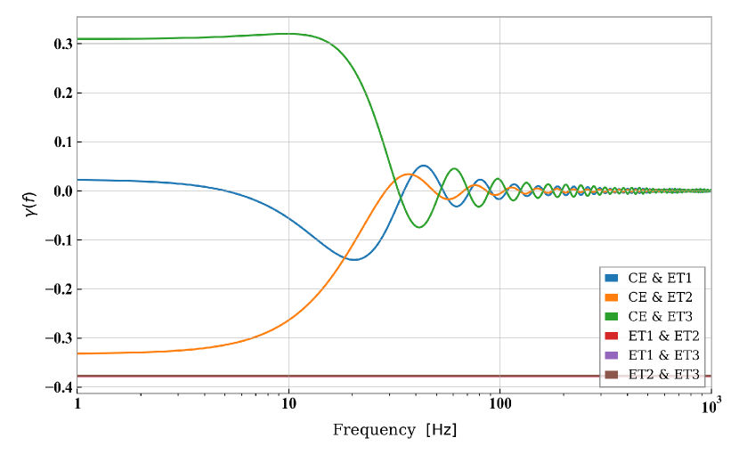
Figure 5: ORF $\gamma(f)$ between Cosmic Explorer (CE) and Einstein Telescope (ET). The ORFs are shown over a logarithmic (top) and linear (bottom) frequency axis. Note that the ORF between different detectors of the ET triangle is constant with a value of about -0.38.

With the definition of the ORF in equation (15), the CPSD between two detectors due to the stochastic GW background can be written Mingarelli et al. (2019)

$$C_{ij}(f)=S_{\rm GW}(f)\gamma_{ij}(f),\quad S_{\rm GW}(f)=\frac{3H_{0}^{2}}{10\pi^{2}}\cdot\frac{\Omega_{\rm GW}(f)}{f^{3}}.$$ (16)

This value needs to be confronted with the average statistical error of the CPSD from uncorrelated instrument noise,

$$\sigma_{ij}(f)=\sqrt{\frac{S_{i}(f)S_{j}(f)}{N}},$$ (17)

where $S_{i}(f)$ is the instrument noise spectral density, and $N$ is the total number of averages going into the estimate of the CPSD. For example, if the total time-stretch of data is $T$, and the CPSD is calculated using segments of length $\tau$ for the fast Fourier transforms (FFTs), and the CPSD calculation foresees the application of spectral windows (anti-leakage), which means that something like 50$\%$ overlap between FFT segments is recommended to make full use of all the information in the data, then we have $N\approx 2T/\tau$.

V.2 Optimal filter

The optimal search for a stochastic background with known or modeled spectral shape involves the integral of CPSDs over frequency. However, since the relative contributions of the stochastic signal and instrument noise to the CPSD vary over frequency, the optimal integration should use a filter $\tilde{Q}_{ij}(f)$, which emphasizes some parts of the spectrum over others.

The signal-to-noise ratio (SNR) of a filtered search is determined by the mean value of the integrated CPSD signals Allen and Romano (1999)

$$\begin{split}\langle\mathcal{C}_{ij}\rangle&=\int\limits_{0}^{\infty}{\rm d}f\,\langle C_{ij}(f)\rangle\tilde{Q}_{ij}(f)\\ &=\int\limits_{0}^{\infty}{\rm d}f\,\gamma_{ij}(f)S_{\rm GW}(f)\tilde{Q}_{ij}(f),\end{split}$$ (18)

and their variances

$$\langle(\mathcal{C}_{ij})^{2}\rangle=\frac{1}{2T}\int\limits_{0}^{\infty}{\rm d}f\,S_{i}(f)S_{j}(f)|\tilde{Q}_{ij}(f)|^{2}.$$ (19)

The averages are over many independent estimates of CPSDs. It is straight-forward to show that the optimal filter function is given by

$$\tilde{Q}_{ij}(f)=\mathcal{N}\frac{\gamma_{ij}^{*}(f)S_{GW}(f)}{S_{i}(f)S_{j}(f)},$$ (20)

where $\mathcal{N}$ is a normalization factor, which has no influence on the SNR. The form of the optimal filters (in arbitrary, but consistent normalization) is shown in figure 6.

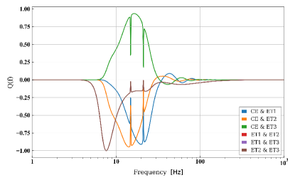
Figure 6: Optimal filter function $\tilde{Q}(f)$ between CE and ET plotted over a logarithmic (top) and linear (bottom) frequency axis. The optimal filters between detectors of the ET triangle are all identical.

In all cases, the optimal filter emphasizes contributions from low frequencies near the lower bound of the observation band of the GW detectors.

Inserting the filter into the previous two equations, we obtain

$${\rm SNR}^{2}=\frac{\langle\mathcal{C}_{ij}\rangle^{2}}{\langle(\mathcal{C}_{ij})^{2}\rangle}=2T\int\limits_{0}^{\infty}{\rm d}f\,\frac{|\gamma_{ij}(f)|^{2}S_{\rm GW}^{2}(f)}{S_{1}(f)S_{2}(f)}$$ (21)

Note that in a discrete version of this equation, the integral becomes a sum over all positive frequency bins, and the ${\rm d}f$ needs to be replaced by $1/\tau$.

Figure 7: Signal-to-noise ratio of a flat $\Omega_{\rm GW}=2\cdot 10^{-12}$ stochastic background. The curves are the SNRs accumulated from high to low frequencies. Total observation time is 1.3 years.

Figure 7 shows the SNR of a flat-$\Omega=2\cdot 10^{-12}$ stochastic background observed over 1.3 years with CE and ET. The curves represent the SNRs accumulated from high to low frequencies, such that the lowest frequency values shown in the plot correspond to the SNR of the correlation measurements making use of all three detectors of an ET triangle. In this way, it is possible to see, at which frequencies most of the SNR is accumulated. Cosmic Explorer correlated with ET is most sensitive to a flat background between 8 Hz and 30 Hz, while ET by itself accumulates its SNR over a slightly broader band. The total SNR achieved by ET in this case is 5.2, while CE correlated with ET achieves an SNR of 3.9.

VI Projection results

The goal is to demonstrate that subtraction residuals can limit the sensitivity of 3G detectors to a CGWB and that the noise-projection method can remove subtraction residuals. In other words, we need to show that subtraction residuals can lie above the instrument-noise contribution of equation (17), and that projection suppresses residuals to a level significantly below the instrument noise.

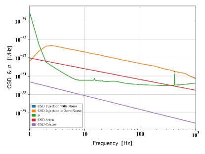
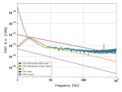
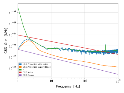
Figure 8: Plots of residual CSDs averaged over all ET detector pairs with BBH foreground (top, left), after best-fit subtraction (top, right), and after noise projection (bottom). The CPSDs are 1.3-year averages and also averaged over all detector pairs of the ET triangle with a total of $10^{6}$ injected BBHs. The astrophysical reference model (red curves) is only an approximation valid below about 100 Hz since it is predicted to fall more strongly above 100 Hz. The purple curve represents a CGWB with frequency independent $\Omega_{\rm GW}=10^{-15}$. The blue curves are the simulated CPSD measurements. The green curves are the predicted instrument noise. The orange curves show the CPSDs for simulations without instrument noise.

We focus this analysis on ET. The CPSDs are calculated from $\tau=2\,$s discrete Fourier transforms using the Welch method with 50% overlap between segments. As stated before, the total simulated time is 1.3 years or $T=4\times 10^{7}$ s. The CPSDs are averaged over all three ET detector pairs. The results are shown in figure 8.

The plots contain reference models of the astrophysical foreground with $\Omega_{GW}=7\times 10^{-10}\times(f/10\rm{Hz})^{2/3}$, which approximates past estimates Regimbau et al. (2017), and a CGWB with frequency independent $\Omega_{GW}=10^{-15}$.

The upper, left plot shows the CPSDs before subtraction of the foreground, the upper, right plot after subtraction, and the bottom plot after projection. The instrument noise of the CPSD (green curve) is calculated using equation (17). In all three plots, the orange curves are the CPSDs from simulations without instrument noise.

The astrophysical BBH foreground shown in the top, left plot (blue curve, hidden behind orange curve) exceeds past predictions (red curve). This is mostly due to the fact that we selected higher-SNR members of the BBH population, for which we expect a Fisher-matrix based projection method to work efficiently. The subtraction residuals in the top, right plot lie above the instrument noise below 10 Hz. It confirms that the sensitivity of ET to a CGWB can be limited by subtraction residuals. This is true for 1.3 years of observation time, and remains true for longer observation times (increasing observation time lowers the instrument noise in these plots, and leaves all other curves the same). Since the spectrum of subtraction residuals depends weakly on the SNRs of the members of the astrophysical foreground (as long as the BBHs can be detected), this conclusion remains valid for more realistic models of the astrophysical foreground. The impact of low-SNR signals, of which only some are detected, or which are included as sub-threshold signal candidates in the subtraction, projection procedure needs to be investigated in future work. The projected residuals (blue curve) in the bottom plot are fully consistent with the instrument-noise model, which means that subtraction residuals were successfully reduced. The full potential of a CGWB search with ET is restored, at least with respect to the higher-SNR signals of a BBH population.

VII Conclusion

In this paper, we presented an analysis of a noise-projection method based on a higher-order geometrical analysis of matched-filter GW searches to mitigate subtraction residuals of an astrophysical foreground in the proposed third-generation detectors Einstein Telescope and Cosmic Explorer. We showed that the projection method can improve the sensitivity to a CGWB. We provided insight into why the projection method is expected to work, and we tested the method with a time-domain simulation of a future detector network. The important first step of the analyses, i.e., the estimation of BBH parameters, was carried out with a state-of-the-art parameter-estimation software (Bilby) by posterior sampling. The presented results are a proof-of-principle since some simplifications of the simulation of the astrophysical foreground had to be done.

The results indicate that the projection method is able to remove all influence of subtraction residuals from BBHs on searches of a CGWB. However, two important aspects need to be addressed in future work. First, the impact of low-SNR signals in the astrophysical foreground on the sensitivity of CGWB searches needs to be investigated. Some of these signals will be visible as sub-threshold signals, others complete hidden in instrumental noise. Their contribution to the astrophysical foreground must be sufficiently low to not pose a fundamental limit to the capacity ET and CE have for CGWB observations. Second, since the foreground removal requires signal models, the dependence of the residuals on choices of waveform models needs to be assessed. Since our implementation of the projection method is fully numerical, we do not require analytical expressions for the waveform models to calculate the projection operators.

VIII Acknowledgement

We are grateful to Cristiano Palomba for providing helpful comments on the manuscript. We acknowledge the use of inference library Bilby for parameter estimation and detector modelling.

References

- Asai et al. (2015) J. Asai et al., Classical and Quantum Gravity 32, 074001 (2015).
- Acernese et al. (2014) F. Acernese et al., Classical and Quantum Gravity 32, 024001 (2014).
- Abbott et al. (2019a) B. P. Abbott, R. Abbott, T. D. Abbott, S. Abraham, F. Acernese, K. Ackley, C. Adams, R. X. Adhikari, V. B. Adya, C. Affeldt, M. Agathos, K. Agatsuma, N. Aggarwal, O. D. Aguiar, L. Aiello, A. Ain, P. Ajith, G. Allen, A. Allocca, M. A. Aloy, P. A. Altin, A. Amato, A. Ananyeva, S. B. Anderson, W. G. Anderson, S. V. Angelova, S. Antier, S. Appert, K. Arai, M. C. Araya, J. S. Areeda, M. Arène, N. Arnaud, K. G. Arun, S. Ascenzi, G. Ashton, S. M. Aston, P. Astone, F. Aubin, P. Aufmuth, K. AultONeal, C. Austin, V. Avendano, A. Avila-Alvarez, S. Babak, P. Bacon, F. Badaracco, M. K. M. Bader, S. Bae, P. T. Baker, F. Baldaccini, G. Ballardin, S. W. Ballmer, S. Banagiri, J. C. Barayoga, S. E. Barclay, B. C. Barish, D. Barker, K. Barkett, S. Barnum, F. Barone, B. Barr, L. Barsotti, M. Barsuglia, D. Barta, J. Bartlett, I. Bartos, R. Bassiri, A. Basti, M. Bawaj, J. C. Bayley, M. Bazzan, B. Bécsy, M. Bejger, et al. (LIGO Scientific Collaboration and Virgo Collaboration), Phys. Rev. X 9, 031040 (2019a).
- Abbott et al. (2009) B. Abbott, R. Abbott, F. Acernese, R. Adhikari, P. Ajith, B. Allen, G. Allen, M. Alshourbagy, R. Amin, S. Anderson, et al., Nature 460, 990 (2009).
- Ade et al. (2018) P. A. R. Ade, Z. Ahmed, R. W. Aikin, K. D. Alexander, D. Barkats, S. J. Benton, C. A. Bischoff, J. J. Bock, R. Bowens-Rubin, J. A. Brevik, I. Buder, E. Bullock, V. Buza, J. Connors, J. Cornelison, B. P. Crill, M. Crumrine, M. Dierickx, L. Duband, C. Dvorkin, J. P. Filippini, S. Fliescher, J. Grayson, G. Hall, M. Halpern, S. Harrison, S. R. Hildebrandt, G. C. Hilton, H. Hui, K. D. Irwin, J. Kang, K. S. Karkare, E. Karpel, J. P. Kaufman, B. G. Keating, S. Kefeli, S. A. Kernasovskiy, J. M. Kovac, C. L. Kuo, N. A. Larsen, K. Lau, E. M. Leitch, M. Lueker, K. G. Megerian, L. Moncelsi, T. Namikawa, C. B. Netterfield, H. T. Nguyen, R. O’Brient, R. W. Ogburn, S. Palladino, C. Pryke, B. Racine, S. Richter, A. Schillaci, R. Schwarz, C. D. Sheehy, A. Soliman, T. St. Germaine, Z. K. Staniszewski, B. Steinbach, R. V. Sudiwala, G. P. Teply, K. L. Thompson, J. E. Tolan, C. Tucker, A. D. Turner, C. Umiltà, A. G. Vieregg, A. Wandui, A. C. Weber, D. V. Wiebe, J. Willmert, C. L. Wong, W. L. K. Wu, H. Yang, K. W. Yoon, and C. Zhang (Keck Array and BICEP2 Collaborations), Phys. Rev. Lett. 121, 221301 (2018).
- Caprini and Figueroa (2018) C. Caprini and D. G. Figueroa, Classical and Quantum Gravity 35, 163001 (2018).
- Christensen (2018) N. Christensen, Reports on Progress in Physics 82, 016903 (2018).
- Turner (1997) M. S. Turner, Phys. Rev. D 55, R435 (1997).
- Easther et al. (2007) R. Easther, J. T. Giblin, and E. A. Lim, Phys. Rev. Lett. 99, 221301 (2007).
- Guzzetti et al. (2016) M. C. Guzzetti, N. Bartolo, M. Liguori, and S. Matarrese, Gravitational waves from inflation (2016), arXiv:1605.01615 [astro-ph.CO] .
- Kamionkowski et al. (1994) M. Kamionkowski, A. Kosowsky, and M. S. Turner, Phys. Rev. D 49, 2837 (1994).
- Kahniashvili et al. (2008) T. Kahniashvili, A. Kosowsky, G. Gogoberidze, and Y. Maravin, Phys. Rev. D 78, 043003 (2008).
- Caprini et al. (2009) C. Caprini, R. Durrer, T. Konstandin, and G. Servant, Phys. Rev. D 79, 083519 (2009).
- Caprini et al. (2016) C. Caprini, M. Hindmarsh, S. Huber, T. Konstandin, J. Kozaczuk, G. Nardini, J. M. No, A. Petiteau, P. Schwaller, G. Servant, and D. J. Weir, Journal of Cosmology and Astroparticle Physics 2016 (04), 001.
- Vachaspati and Vilenkin (1985) T. Vachaspati and A. Vilenkin, Phys. Rev. D 31, 3052 (1985).
- Damour and Vilenkin (2005) T. Damour and A. Vilenkin, Phys. Rev. D 71, 063510 (2005).
- Siemens et al. (2007) X. Siemens, V. Mandic, and J. Creighton, Phys. Rev. Lett. 98, 111101 (2007).
- Ölmez et al. (2010) S. Ölmez, V. Mandic, and X. Siemens, Phys. Rev. D 81, 104028 (2010).
- Crowder and Cornish (2005) J. Crowder and N. J. Cornish, Phys. Rev. D 72, 083005 (2005).
- Kawamura et al. (2006) S. Kawamura et al., Classical and Quantum Gravity 23, S125 (2006).
- Punturo et al. (2010) M. Punturo, M. Abernathy, F. Acernese, B. Allen, N. Andersson, K. Arun, F. Barone, B. Barr, M. Barsuglia, M. Beker, N. Beveridge, S. Birindelli, S. Bose, L. Bosi, S. Braccini, C. Bradaschia, T. Bulik, E. Calloni, G. Cella, E. C. Mottin, S. Chelkowski, A. Chincarini, J. Clark, E. Coccia, C. Colacino, J. Colas, A. Cumming, L. Cunningham, E. Cuoco, S. Danilishin, K. Danzmann, G. D. Luca, R. D. Salvo, T. Dent, R. D. Rosa, L. D. Fiore, A. D. Virgilio, M. Doets, V. Fafone, P. Falferi, R. Flaminio, J. Franc, F. Frasconi, A. Freise, P. Fulda, J. Gair, G. Gemme, A. Gennai, A. Giazotto, K. Glampedakis, M. Granata, H. Grote, G. Guidi, G. Hammond, M. Hannam, J. Harms, D. Heinert, M. Hendry, I. Heng, E. Hennes, S. Hild, J. Hough, S. Husa, S. Huttner, G. Jones, F. Khalili, K. Kokeyama, K. Kokkotas, B. Krishnan, M. Lorenzini, H. Lück, E. Majorana, I. Mandel, V. Mandic, I. Martin, C. Michel, Y. Minenkov, N. Morgado, S. Mosca, B. Mours, H. Müller-Ebhardt, P. Murray, R. Nawrodt, J. Nelson, R. Oshaughnessy, C. D. Ott, C. Palomba, A. Paoli, G. Parguez, A. Pasqualetti, R. Passaquieti, D. Passuello, L. Pinard, R. Poggiani, P. Popolizio, M. Prato, P. Puppo, D. Rabeling, P. Rapagnani, J. Read, T. Regimbau, H. Rehbein, S. Reid, L. Rezzolla, F. Ricci, F. Richard, A. Rocchi, S. Rowan, A. Rüdiger, B. Sassolas, B. Sathyaprakash, R. Schnabel, C. Schwarz, P. Seidel, A. Sintes, K. Somiya, F. Speirits, K. Strain, S. Strigin, P. Sutton, S. Tarabrin, A. Thüring, J. van den Brand, C. van Leewen, M. van Veggel, C. van den Broeck, A. Vecchio, J. Veitch, F. Vetrano, A. Vicere, S. Vyatchanin, B. Willke, G. Woan, P. Wolfango, and K. Yamamoto, Classical and Quantum Gravity 27, 194002 (2010).
- Reitze et al. (2019) D. Reitze, R. X. Adhikari, S. Ballmer, B. Barish, L. Barsotti, G. Billingsley, D. A. Brown, Y. Chen, D. Coyne, R. Eisenstein, M. Evans, P. Fritschel, E. D. Hall, A. Lazzarini, G. Lovelace, J. Read, B. S. Sathyaprakash, D. Shoemaker, J. Smith, C. Torrie, S. Vitale, R. Weiss, C. Wipf, and M. Zucker, Cosmic explorer: The u.s. contribution to gravitational-wave astronomy beyond ligo (2019), arXiv:1907.04833 [astro-ph.IM] .
- Thrane et al. (2013) E. Thrane, N. Christensen, and R. M. S. Schofield, Phys. Rev. D 87, 123009 (2013).
- Coughlin et al. (2016) M. W. Coughlin, N. L. Christensen, R. D. Rosa, I. Fiori, M. Gołkowski, M. Guidry, J. Harms, J. Kubisz, A. Kulak, J. Mlynarczyk, F. Paoletti, and E. Thrane, Classical and Quantum Gravity 33, 224003 (2016).
- Christensen (1992) N. Christensen, Phys. Rev. D 46, 5250 (1992).
- Allen and Romano (1999) B. Allen and J. D. Romano, Phys. Rev. D 59, 102001 (1999).
- Ballmer (2006) S. W. Ballmer, Classical and Quantum Gravity 23, S179 (2006).
- Romano (2019) J. D. Romano, Searches for stochastic gravitational-wave backgrounds (2019), arXiv:1909.00269 [gr-qc] .
- Vangioni et al. (2015) E. Vangioni, K. A. Olive, T. Prestegard, J. Silk, P. Petitjean, and V. Mandic, Monthly Notices of the Royal Astronomical Society 447, 2575 (2015), https://academic.oup.com/mnras/article-pdf/447/3/2575/9385019/stu2600.pdf .
- Belczynski et al. (2002) K. Belczynski, V. Kalogera, and T. Bulik, The Astrophysical Journal 572, 407 (2002).
- Vitale et al. (2019) S. Vitale, W. M. Farr, K. K. Y. Ng, and C. L. Rodriguez, The Astrophysical Journal 886, L1 (2019).
- Regimbau et al. (2017) T. Regimbau, M. Evans, N. Christensen, E. Katsavounidis, B. Sathyaprakash, and S. Vitale, Phys. Rev. Lett. 118, 151105 (2017).
- Sachdev et al. (2020) S. Sachdev, T. Regimbau, and B. S. Sathyaprakash, Subtracting compact binary foreground sources to reveal primordial gravitational-wave backgrounds (2020), arXiv:2002.05365 [gr-qc] .
- Cutler and Harms (2006) C. Cutler and J. Harms, Phys. Rev. D 73, 042001 (2006).
- Harms et al. (2008) J. Harms, C. Mahrdt, M. Otto, and M. Prieß, Phys. Rev. D 77, 123010 (2008).
- Smith and Thrane (2018) R. Smith and E. Thrane, Phys. Rev. X 8, 021019 (2018).
- Abbott et al. (2017) B. P. Abbott, R. Abbott, T. D. Abbott, M. R. Abernathy, K. Ackley, C. Adams, P. Addesso, R. X. Adhikari, V. B. Adya, C. Affeldt, N. Aggarwal, O. D. Aguiar, A. Ain, P. Ajith, B. Allen, P. A. Altin, S. B. Anderson, W. G. Anderson, K. Arai, M. C. Araya, C. C. Arceneaux, J. S. Areeda, K. G. Arun, G. Ashton, M. Ast, S. M. Aston, P. Aufmuth, C. Aulbert, S. Babak, P. T. Baker, S. W. Ballmer, J. C. Barayoga, S. E. Barclay, B. C. Barish, D. Barker, B. Barr, L. Barsotti, J. Bartlett, I. Bartos, R. Bassiri, et al., Classical and Quantum Gravity 34, 044001 (2017).
- Akutsu et al. (2019) T. Akutsu et al. (KAGRA), Nature Astronomy 3, 35 (2019).
- Souradeep (2016) T. Souradeep, Resonance 21, 225 (2016).
- 3Gs (2019) Gravitational-Wave Astronomy with the Next-Generation Earth-Based Observatories (2019).
- Maggiore et al. (2019) M. Maggiore, C. van den Broeck, N. Bartolo, E. Belgacem, D. Bertacca, M. A. Bizouard, M. Branchesi, S. Clesse, S. Foffa, J. García-Bellido, S. Grimm, J. Harms, T. Hinderer, S. Matarrese, C. Palomba, M. Peloso, A. Ricciardone, and M. Sakellariadou, Science Case for the Einstein Telescope (2019), arXiv:1912.02622 [astro-ph.CO] .
- Hild et al. (2011) S. Hild, M. Abernathy, F. Acernese, P. Amaro-Seoane, N. Andersson, K. Arun, F. Barone, B. Barr, M. Barsuglia, M. Beker, N. Beveridge, S. Birindelli, S. Bose, L. Bosi, S. Braccini, C. Bradaschia, T. Bulik, E. Calloni, G. Cella, E. C. Mottin, S. Chelkowski, A. Chincarini, J. Clark, E. Coccia, C. Colacino, J. Colas, A. Cumming, L. Cunningham, E. Cuoco, S. Danilishin, K. Danzmann, R. D. Salvo, T. Dent, R. D. Rosa, L. D. Fiore, A. D. Virgilio, M. Doets, V. Fafone, P. Falferi, R. Flaminio, J. Franc, F. Frasconi, A. Freise, D. Friedrich, P. Fulda, J. Gair, G. Gemme, E. Genin, A. Gennai, A. Giazotto, K. Glampedakis, C. Gräf, M. Granata, H. Grote, G. Guidi, A. Gurkovsky, G. Hammond, M. Hannam, J. Harms, D. Heinert, M. Hendry, I. Heng, E. Hennes, J. Hough, S. Husa, S. Huttner, G. Jones, F. Khalili, K. Kokeyama, K. Kokkotas, B. Krishnan, T. G. F. Li, M. Lorenzini, H. Lück, E. Majorana, I. Mandel, V. Mandic, M. Mantovani, I. Martin, C. Michel, Y. Minenkov, N. Morgado, S. Mosca, B. Mours, H. Müller-Ebhardt, P. Murray, R. Nawrodt, J. Nelson, R. Oshaughnessy, C. D. Ott, C. Palomba, A. Paoli, G. Parguez, A. Pasqualetti, R. Passaquieti, D. Passuello, L. Pinard, W. Plastino, R. Poggiani, P. Popolizio, M. Prato, M. Punturo, P. Puppo, D. Rabeling, P. Rapagnani, J. Read, T. Regimbau, H. Rehbein, S. Reid, F. Ricci, F. Richard, A. Rocchi, S. Rowan, A. Rüdiger, L. SantamarÃa, B. Sassolas, B. Sathyaprakash, R. Schnabel, C. Schwarz, P. Seidel, A. Sintes, K. Somiya, F. Speirits, K. Strain, S. Strigin, P. Sutton, S. Tarabrin, A. Thüring, J. van den Brand, M. van Veggel, C. van den Broeck, A. Vecchio, J. Veitch, F. Vetrano, A. Vicere, S. Vyatchanin, B. Willke, G. Woan, and K. Yamamoto, Classical and Quantum Gravity 28, 094013 (2011).
- Hild et al. (2009) S. Hild, S. Chelkowski, A. Freise, J. Franc, N. Morgado, R. Flaminio, and R. DeSalvo, Classical and Quantum Gravity 27, 015003 (2009).
- Ashton et al. (2019) G. Ashton, M. Hübner, P. D. Lasky, C. Talbot, K. Ackley, S. Biscoveanu, Q. Chu, A. Divakarla, P. J. Easter, B. Goncharov, F. H. Vivanco, J. Harms, M. E. Lower, G. D. Meadors, D. Melchor, E. Payne, M. D. Pitkin, J. Powell, N. Sarin, R. J. E. Smith, and E. Thrane, The Astrophysical Journal Supplement Series 241, 27 (2019).
- Adams et al. (2016) T. Adams, D. Buskulic, V. Germain, G. M. Guidi, F. Marion, M. Montani, B. Mours, F. Piergiovanni, and G. Wang, Classical and Quantum Gravity 33, 175012 (2016).
- Vinciguerra et al. (2017) S. Vinciguerra, J. Veitch, and I. Mandel, Classical and Quantum Gravity 34, 115006 (2017).
- Abbott et al. (2019b) B. Abbott et al., The Astrophysical Journal 882, L24 (2019b).
- Danzmann et al. (2017) K. Danzmann et al., (2017), 1702.00786 .
- Ade et al. (2016) P. A. R. Ade et al., Astronomy and Astrophysics 594, 10.1051/0004-6361/201525830 (2016).
- Abbott et al. (2019) B. P. Abbott et al. (LIGO Scientific and Virgo Collaboration), Phys. Rev. D 100, 061101 (2019).
- Nishizawa et al. (2009) A. Nishizawa, A. Taruya, K. Hayama, S. Kawamura, and M.-a. Sakagami, Phys. Rev. D 79, 082002 (2009).
- Cella (2000) G. Cella, in Recent Developments in General Relativity, edited by B. Casciaro, D. Fortunato, M. Francaviglia, and A. Masiello (Springer Milan, 2000) pp. 495–503.
- Coughlin et al. (2018) M. W. Coughlin, A. Cirone, P. Meyers, S. Atsuta, V. Boschi, A. Chincarini, N. L. Christensen, R. De Rosa, A. Effler, I. Fiori, M. Gołkowski, M. Guidry, J. Harms, K. Hayama, Y. Kataoka, J. Kubisz, A. Kulak, M. Laxen, A. Matas, J. Mlynarczyk, T. Ogawa, F. Paoletti, J. Salvador, R. Schofield, K. Somiya, and E. Thrane, Phys. Rev. D 97, 102007 (2018).
- Regimbau et al. (2012) T. Regimbau, T. Dent, W. Del Pozzo, S. Giampanis, T. G. F. Li, C. Robinson, C. Van Den Broeck, D. Meacher, C. Rodriguez, B. S. Sathyaprakash, and K. Wójcik, Phys. Rev. D 86, 122001 (2012).
- Mingarelli et al. (2019) C. M. F. Mingarelli, S. R. Taylor, B. S. Sathyaprakash, and W. M. Farr, Understanding in gravitational wave experiments (2019), arXiv:1911.09745 [gr-qc] .