Machine Learning Etudes in Conformal Field Theories

Abstract

We demonstrate that various aspects of Conformal Field Theory are amenable to machine learning. Relatively modest feed-forward neural networks are able to distinguish between scale and conformal invariance of a three-point function and identify a crossing-symmetric four-point function to nearly a hundred percent accuracy. Furthermore, neural networks are also able to identify conformal blocks appearing in a putative CFT four-point function and predict the values of the corresponding OPE coefficients. Neural networks also successfully classify primary operators by their quantum numbers under discrete symmetries in the CFT from examining OPE data. We also demonstrate that neural networks are able to learn the available OPE data for scalar correlation function in the 3d Ising model and predict the twists of higher-spin operators that appear in scalar OPE channels by regression.

1 Introduction and Summary

Conformal Field Theories (CFTs) are a particularly interesting and important class of Quantum Field Theories, both from a theoretical and a phenomenological point of view. For example, as is well known, they are the natural language to describe physical systems undergoing phase transitions. Furthermore, in two space-time dimensions, they admit a great deal of analytic control due to the presence of an infinite dimensional Virasoro symmetry. In higher than two dimensions, there have also been been significant advances ranging from the discovery of new bose-fermi symmetries in three dimensions Polyakov:1988md ; Shaji:1990is ; Fradkin:1994tt ; Giombi:2011kc ; Aharony:2011jz ; Aharony:2012nh , duality to higher-spin theories in Anti-de Sitter spaces Klebanov:2002ja ; Sezgin:2002rt ; Gaberdiel:2010pz ; Beccaria:2014zma ; Bae:2016hfy , as well as a large amount of work in computing the physical data (i.e. spectrum, OPE coefficients) of a given field theory both numerically Rychkov:2011et ; ElShowk:2012ht ; El-Showk:2014dwa ; Kos:2016ysd ; Simmons-Duffin:2016wlq ; Chester:2019ifh ; Rong:2017cow ; Stergiou:2018gjj , and analytically Beem:2014zpa ; Beem:2015aoa ; Alday:2016njk ; Gopakumar:2016cpb ; Alday:2017zzv ; Aharony:2018npf .

An important driver in this progress has been the theoretical and numerical advancements in the conformal bootstrap in greater than two dimensions. Hence we now have the tools to access a large amount of precise physical data for CFTs in various dimensions, along with their rich theoretical structures. With the further advances in computational ability, and the conceptual progress in conformal bootstrap methods, one may optimistically expect these developments will usher the usage of machine-learning (ML) techniques in the studies of conformal field theories. Such an approach is very much in line with the programme of He:2017aed ; He:2017set to machine-learn structures arising in theoretical physics and pure mathematics without the neural network been given any prior knowledge of the underlying mathematics. Indeed, He:2017aed ; He:2017set ; Krefl:2017yox ; Ruehle:2017mzq ; Carifio:2017bov ; Erbin:2018csv brought ML to string theory. The reader is also referred to Hashimoto:2018ftp for the fascinating idea that space-time itself might be a neural network, as well as the introductory books He:2018jtw ; RUEHLE20201 (the monograph RUEHLE20201 is an excellent technical introduction of ML to theoretical physicists). Further interesting applications of ML to string theory, supergravity and quantum field theory are Comsa:2019rcz ; Krishnan:2020sfg ; Chernodub:2019kon ; Chernodub:2020nip .

In this paper, we shall take some initial steps in applying the methods from machine learning to analyze the data already available to us. The aim is to build up a toolbox which we hope will become useful in tackling wide range of interesting physical problems in conformal field theories. We will demonstrate that several definitive features of conformal field theories, from their general structures to the physical data for the systems of particular importance are indeed machine learnable.

We begin with a warm-up subsection 2.1, where we demonstrate that machine is capable of learning to classify even and odd functions, as well as functions with antipodal symmetries. In subsection 2.2, we will show that machine learning algorithms perform well on recognizing the presence of conformal symmetry in a putative system as they can distinguish the scale and conformal invariant two and three-point functions of scalar operators to near hundred percent accuracy. As shown in subsection 2.3, these algorithms are also able to recognize the crossing symmetric four-point functions again with a near hundred percent accuracy.

We next turn to Section 3 where we focus on extracting more fine-grained information about conformal symmetry as carried by a putative four-point function. In particular, we demonstrate in a simple context that neural networks can predict the value of the particular OPE coefficient appearing in front of a conformal block to reasonable accuracy. As a warm-up to this, we consider the same problem, but for the Fourier expansion of an arbitrary function. We also find along the way that neural networks can easily identify classes of functions where a particular conformal block or Fourier mode is missing in the expansion. This somewhat curious and unexpected property however can be understood from a Principal Component analysis, as we also show. This serves as the first step towards applying machine-learning techniques to tackle fully-fledged conformal bootstrap problems.

Furthermore, we show in subsection 4.2, that these algorithms also perform well on the occurrence of discrete symmetries in the theory. They are able to, for instance, organize the (partial) spectrum of the 3d Ising model into $\mathbb{Z}_{2}$ even and odd operators from the knowledge of their OPE coefficients. From trial explorations, we expect that these algorithms should also perform well when the discrete symmetry is more complicated than $\mathbb{Z}_{2}$. The reader is also referred to Betzler:2020rfg ; Bao:2020nbi ; He:2020eva for the usage of ML in recognizing dualities in QFTs.

We also consider another possible utility of ML algorithms, now in the context of the conformal bootstrap. The state of the art numerical method involves reducing the crossing equations to a semi-definite programming problem which is then solved numerically Simmons-Duffin:2015qma ; Landry:2019qug , see Poland:2018epd for a review. While this yields extremely accurate results on the numerical bounds of CFT data, it can be computationally expensive. In this case, can machine-learning methods assist us in extracting more about the spectrum of the CFT? We can answer this question in the affirmative, at least for the $[\sigma\sigma]_{0}$ and $[\sigma\epsilon]_{0}$ operator families in the 3d Ising Model, where machine-learning methods are able to train on the existing numerical data and provide regression curves with good extrapolation. Though this is a baby example where the curve is somewhat simple, and indeed even the analytic expressions are known, it is an important proof-of-concept. We especially emphasize here that machine-learning regression analysis does not require us to input a form of the trial curve by hand. One may therefore expect that we could carry out a similar analysis even when the form of the data set is more complicated and it is not obvious if a standard curve-fitting based regression analysis would be feasible. Indeed, these are precisely the cases where machine-learning methods shine, see for example Ashmore:2019wzb , where simple, generic neural networks improve the known Donaldson algorithm for numerical Calabi-Yau metrics by almost 2 orders of magnitude.

Our motivation for these analyses is the fact that machine learning has made important contributions in various physical and mathematical problems in the recent past, see MEHTA20191 ; He:2018jtw ; Bao:2020sqg ; RUEHLE20201 for reviews and references. In addition, machine learning methods have now started to routinely compete with and even outperform existing numerical and analytical methods in mathematics and physics sirignano2018dgm ; Piscopo:2019txs ; Ashmore:2019wzb ; broecker2017machine . It would therefore be of great interest to apply machine learning methods to analyze CFTs. However, at the same time one must note that often failure modes of machine learning are not very well understood, and it is a priori not obvious whether a problem is machine learnable or not. The computations we present here indicate, at least at the level of proof-of-concept, that machine learning methods can be useful tools to have at hand when exploring conformal field theories.

Finally, the results we have presented in this paper are obtained using mainly neural networks, both for classification and regression problems. This is an idiosyncratic choice made mainly for reasons of definiteness, and eventually we hope to analyse truly large amounts of CFT data using these methods in near future. Neural networks are a flexible framework which scale well with large amounts of data. More traditional machine learning methods such as support vector machines and decision trees do also perform comparably well on the problems we have addressed here.

We provide a summary of the classification and regression problems we have carried out in Table 1.

Classification Problem	Accuracy at 80/20 Split
Even/Odd Functions	$100\%$
Plane/Antipodal/Null Reflection Symmetries	$99.66\%$
Scale vs Conformal Invariance: three-point functions	$89.99\%$
Scale vs Conformal Invariance: two & three-point functions	$99.00\%$
Recognizing Crossing Symmetric four-point functions	$100\%$
Fourier Series Expansions	$98.00\%$
Conformal Block Expansions	$97.00\%$
$\mathbb{Z}_{2}$ symmetry of the Ising Model	$100\%$
$\mathbb{Z}_{3}$ discrete symmetry	$99.73\%$

Regression Problem	R-squared Value
Predicing value of Fourier Coefficient	0.9999
Predicting value of OPE coefficient	0.9988
Predicting $\tau_{[\sigma\sigma]_{0}}(\bar{h})$ for the 3d Ising model	tanh ansatz: 1.0 Neural Network: 0.9804
Predicting $\tau_{[\sigma\epsilon]_{0}}(\bar{h})$ for even-spin operators	tanh ansatz: 1.0 Neural Network: 0.9966
Predicting $\tau_{[\sigma\epsilon]_{0}}(\bar{h})$ for odd-spin operators	tanh ansatz: 1.0 Neural Network: 0.9926

Table 1: The classification and regression problems done in this paper evaluated by accuracy and r-squared value respectively. A value of r-square close to one indicates a good prediction by the regressor.

Note: While preparing this draft, we learned of the interesting paper Krippendorf:2020gny which also studies identification of symmetries in data sets by means of neural networks. Like the authors of Krippendorf:2020gny , we also find principal component analysis to be a useful tool to gain insight into symmetries. It would be interesting to compare the two approaches in greater detail, and we hope to return to this question in the future.

2 Detecting Symmetries using Neural Networks

We begin with demonstrating how neural networks may be trained to detect the presence of various discrete symmetries in real valued functions. To the best of our knowledge, these observations, which pave the way to our study of scale and conformal symmetries in the correlation functions, are new.

As an aside, we would like to first make the following observation. Typically in ‘visual’ classification problems that neural networks are trained for, e.g. cat vs dog classifiers, or face detection and recognition, the neural network has multiple hidden layers and typically also convolutional layers (see e.g. 726791 ; 10.5555/2999134.2999257 ) in order to have the best possibility to capture fine local correlations in the image, and to transfer learning from one patch in the image to another patch and so on. In the classification problems we study here, there are no local correlations that we study or allow for. The functions are randomly generated point clouds that obey particular global properties. This is done with a view to ensuring that the classifier indeed learns the given global properties of the function we are trying to teach it, and is not reliant on spurious or accidental local correlations. This also leads us to expect that we could successfully work with shallow fully connected neural networks for our classification tasks. Indeed, such networks prove to suffice in what follows.

2.1 Classifying Discrete Symmetries

One of the simplest symmetry properties a real-valued mono-variate function may have is to be even or odd under the change of sign of its argument. We therefore consider two classes of functions, viz.

$$\left\{f(x):f(-x)=f(x)\right\}\qquad\text{and}\qquad\left\{f(x):f(-x)=-f(x)\right\}\,,$$ (1)

and train a neural network to classify functions under this property. The training data for the neural network is defined in Table 2.

$\mathrm{Point\,Cloud}$	$\mathrm{X}$	$\mathrm{Y}$
$\mathrm{Even\,Function}$	$\left(\mathbf{x},\mathbf{f(x)},\,-\mathbf{x},\mathbf{f(x)}\right)$	$\left(1,0\right)$
$\mathrm{Odd\,Function}$	$\left(\mathbf{x},\mathbf{f(x)},\,-\mathbf{x},-\mathbf{f(x)}\right)$	$\left(0,1\right)$

Table 2: The training data for the even-odd classification problem. $\mathbf{x}$ and $\mathbf{f(x)}$ are 64 dimensional vectors of normally distributed random numbers taking values in $\left[0,\pi\right]$ and $\left[-1,1\right]$ respectively. The neural network was trained on 10000 instances of this data.

The Neural Network trained on this data set is described in Figure 3(a). It was trained for 4 epochs and achieved a hundred percent accuracy. The accuracy and loss curves are shown in Figure 1.

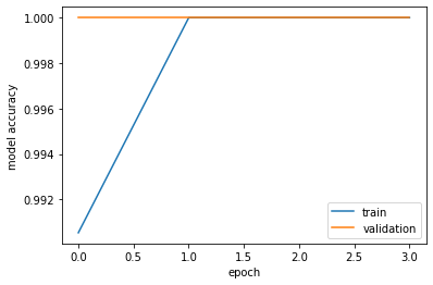
(a) Accuracy

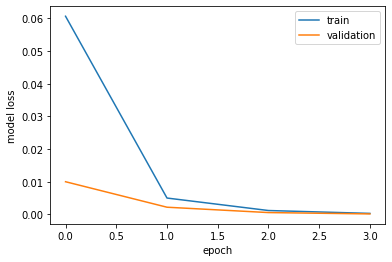
(b) Loss

Figure 1: The Accuracy and Loss curves for the Even-Odd Classifier Neural Network. The data set was organized into training and validation sets in an 80/20 split.

As an extension of the above classification, one may similarly consider classes of three-dimensional point clouds with the various symmetry properties. Firstly, we consider reflection symmetry about the $x-y$ plane, secondly, we consider antipodal reflection symmetry and finally, point clouds which are completely randomly generated, with no symmetries. The purpose of having a null case for the classifier is to test that it is indeed capable of distinguishing the point clouds with definite symmetry properties and those without. These symmetries and the corresponding data set are enumerated in Table 3, and the corresponding neural network classifier is summarized in Figure 3(b). The Neural Network classifier could classify point clouds to 0.995 accuracy, as may be seen from the accuracy curve in Figure 2.

We remark, whilst on the subject of simple discrete symmetries, that we can try an even simpler problem. Can a classifier learn modulo arithmetic? Suppose we fix a number $p$ and establish a labelled data-set $\{n_{i}\}\rightarrow n\mod p$, where $n_{i}$ is the list of digits of $n$ in some base (it turn out that which base is not important here). A simple classifier such as logistic regression, or a neural network such as a multi-layer perceptron with a linear layer and a sigmoid layer will very quickly “learn” this to accuracy and confidence very close to 1 for $p=2$ (even/odd). The higher the $p$, the more the categories to classify, and the accuracies decrease as expected. Furthermore, if we do not fix $p$ and feed the classifier with pairs $(n,p)$ all mixed up, then, the accuracies are nearly zero. This is very much in line with the experiments of He:2017set that the moment primes are involved, simple neural-network techniques expectantly fail in recognizing any patterns. Nevertheless, in experiments in finite groups theory, and in arithmetic geometry have met with greater success Alessandretti:2019jbs ; He:2019nzx .

Point Cloud Symmetry	$\mathrm{X}$	$\mathrm{Y}$
Plane Reflection	$\left(\mathbf{x},\mathbf{y},\mathbf{z}\right)\,\cup\,\left(\mathbf{x},\mathbf{y},-\mathbf{z}\right)$	$\left(1,0,0\right)$
Antipodal Reflection	$\left(\mathbf{x},\mathbf{y},\mathbf{z}\right)\,\cup\,\left(-\mathbf{x},-\mathbf{y},-\mathbf{z}\right)$	$\left(0,1,0\right)$
Null	$\left(\mathbf{x}_{1},\mathbf{y}_{1},\mathbf{z}_{1}\right)\,\cup\,\left(\mathbf{x}_{2},\mathbf{y}_{2},\mathbf{z}_{2}\right)$	$\left(0,0,1\right)$

Table 3: The training data for the three-dimensional point cloud classification problem. $\mathbf{x}$, $\mathbf{y}$ and $\mathbf{z}$ are 200 dimensional vectors of normally distributed random numbers taking values in $\left[-1,1\right]$. The neural network was trained on 10000 instances of this data.

(a) Accuracy

(b) Loss

Figure 2: The Accuracy and Loss curves for the Neural Network learning the point cloud symmetries of Table 3. The data set was organized into training and validation sets in an 80/20 split.

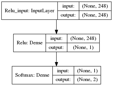
(a) Even-Odd Classifier

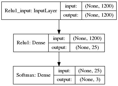
(b) 3d Symmetry Classifier

Figure 3: The Neural Networks for classifying even/odd functions and three-dimensional symmetries. The first has a total of 253 trainable parameters, while the second has a total of 30,103 trainable parameters.

2.2 Scale Invariance vs Conformal Invariance

We next turn to study how neural networks may be trained to distinguish between scale invariance and conformal invariance from the correlation functions exhibiting either of these symmetries. This can be useful for machine to distinguish the emergence of scale or conformal symmetries in condensed matter systems.

Let us briefly review the relevant details about scale and conformal invariant correlation functions we will perform the machine-learning. Given a quantum field theory in $d$-dimensional space-time, containing scalar operators $\mathcal{O}_{1}$, $\mathcal{O}_{2}$ and $\mathcal{O}_{3}$ of scaling dimensions $\Delta_{1}$, $\Delta_{2}$ and $\Delta_{3}$ respectively, the two point function is constrained by scale invariance to be of the form Nakayama:2013is :

$$\left\langle\mathcal{O}_{\Delta_{i}}\left(x_{1}\right)\mathcal{O}_{\Delta_{j}}\left(x_{2}\right)\right\rangle=\frac{c_{ij}}{\left|x_{12}\right|^{\Delta_{i}+\Delta_{j}}}\,,\quad x_{ij}=x_{i}-x_{j},$$ (2)

where $|x_{ij}|=\sqrt{(x_{i}-x_{j})^{2}}$ and $c_{ij}$ is an overall normalization constant. Requiring conformal invariance imposes the additional two point orthogonality condition such that $c_{ij}=c^{(i)}\delta_{ij}$. Additionally, conformal invariance imposes even more restrictive constraints on the three-point correlation functions of the theory. In particular, if the theory has only scale invariance, the form of the three-point function is fixed to be:

$$\begin{split}&\left\langle\mathcal{O}_{\Delta_{1}}\left(x_{1}\right)\mathcal{O}_{\Delta_{2}}\left(x_{2}\right)\mathcal{O}_{\Delta_{3}}\left(x_{3}\right)\right\rangle=\sum_{\{a,b,c\}}{c_{abc}\over\left|x_{12}\right|^{a}\left|x_{23}\right|^{b}\left|x_{31}\right|^{c}}\,,\\ &\qquad a+b+c=\Delta_{1}+\Delta_{2}+\Delta_{3}\,,\end{split}$$ (3)

where $a$, $b$ and $c$ are positive real numbers, constrained as above. On the other hand, if the theory has full conformal invariance, then exponents of $x_{ij}$ in the three-point function are completely determined, i.e.

$$\left\langle\mathcal{O}_{\Delta_{1}}\left(x_{1}\right)\mathcal{O}_{\Delta_{2}}\left(x_{2}\right)\mathcal{O}_{\Delta_{3}}\left(x_{3}\right)\right\rangle={\lambda_{123}\over\left|x_{12}\right|^{\alpha_{123}}\left|x_{23}\right|^{\alpha_{231}}\left|x_{31}\right|^{\alpha_{312}}}\,,$$ (4)

where $\alpha_{ijk}=\Delta_{i}+\Delta_{j}-\Delta_{k}$ and $\lambda_{ijk}$ is known as the OPE coefficient.

We shall begin with a simple classification problem, where we supply the neural network outlined in Figure 6 a point cloud of positions $x_{1}$, $x_{2}$, $x_{3}$, and quantum numbers $\Delta_{i}$ of the three operators. We consider the two classes of functions given in Equations (3) and (4) and train the classifier to distinguish between the two functions. Our training set is explained in greater detail in Table 4, and the training curves for the neural network are shown in Figure 4, from where it is apparent that the classifier can easily train up to around 95 percent accuracy. Subsequently, we generated a new set of testing data of three-point functions for the classifier, and found that the neural network could classify these functions, which had not been used for training or validation, to 97.15 percent accuracy.

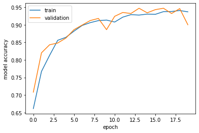
(a) Accuracy

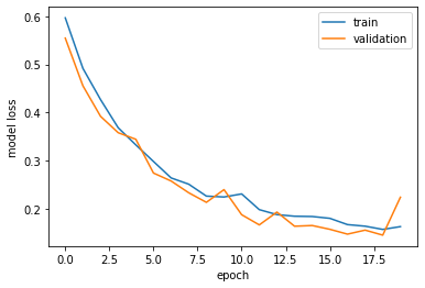
(b) Loss

Figure 4: The Accuracy and Loss curves for the Scale vs Conformal Invariance classification when the Neural Network in Figure 6 is fed the conformal dimensions along with the corresponding three-point correlation functions. Training and validation sets are constructed with an 80/20 split.

$\mathrm{Symmetry}$	$\mathrm{X}$	$\mathrm{Y}$
$\mathrm{Scale\,Invariance}$	$\left(\mathbf{x}_{12},\mathbf{x}_{23},\mathbf{x}_{31},\Delta_{1},\Delta_{2},\Delta_{3},f^{(3)}_{scale}\right)_{(100)}$	$\left(1,0\right)$
$\mathrm{Conformal\,Invariance}$	$\left(\mathbf{x}_{12},\mathbf{x}_{23},\mathbf{x}_{31},\Delta_{1},\Delta_{2},\Delta_{3},f^{(3)}_{cft}\right)_{(100)}$	$\left(0,1\right)$

Table 4: The first set of training data for the classification of scale and conformal invariant correlation functions. $x_{ij}$ is the invariant distance $\sqrt{\left(x_{i}-x_{j}\right)^{2}}$ and the $\Delta_{i}$ are the conformal dimensions of the operators $\mathcal{O}_{i}$ positioned at $x_{i}$. The three-point functions $f^{(3)}_{cft}$ and $f^{(3)}_{cft}$ are defined in (3) and (4) respectively. For each training instance, $a$, $b$ and $c$ are chosen randomly to satisfy the constraint in (3). The subscript (100) indicates that each such instance of training data is a $100\times 7$ array. This is flattened into a 700 dimensional vector and fed to the neural network along with its value of $Y$ as a single training instance. The neural network was trained on 10000 instances of this data, i.e. 5000 scale invariant functions and 5000 conformal invariant functions.

It turns out that one may improve the classifier performance by an alteration in how the training data is presented to it. Next, rather than supplying the classifier the conformal dimensions of operators and the three-point function, we supplied it two-point functions of each operator, along with the three-point function. The neural network could distinguish between a randomly generated set of scale and conformally invariant correlation functions that it had not been trained on to 99.00 percent accuracy.

$\mathrm{Symmetry}$	$\mathrm{X}$	$\mathrm{Y}$
$\mathrm{Scale\,Invariance}$	$\left(\mathbf{x}_{12},\mathbf{x}_{23},\mathbf{x}_{31},f^{(2)}_{\Delta_{1}},f^{(2)}_{\Delta_{2}},f^{(2)}_{\Delta_{3}},f^{(3)}_{\rm scale}\right)_{(100)}$	$\left(1,0\right)$
$\mathrm{Conformal\,Invariance}$	$\left(\mathbf{x}_{12},\mathbf{x}_{23},\mathbf{x}_{31},f^{(2)}_{\Delta_{1}},f^{(2)}_{\Delta_{2}},f^{(2)}_{\Delta_{3}},f^{(3)}_{\rm conformal}\right)_{(100)}$	$\left(0,1\right)$

Table 5: The second set of training data for the classification of scale and conformal invariant correlation functions. Instead of passing the conformal dimensions $\Delta_{i}$ as done previously, we pass it the point cloud of the respective two point correlation functions. The neural network was trained on 10000 instances of this data, i.e. 5000 scale invariant functions and 5000 conformal invariant functions.

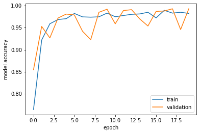
(a) Accuracy

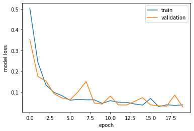
(b) Loss

Figure 5: The Accuracy and Loss curves for the Scale vs Conformal Invariance classification when the Neural Network in Figure 6 is fed a point-cloud of two-point and three-point correlation functions. Training and validation sets are constructed with an 80/20 split.

The learning curves are in Figure 5.

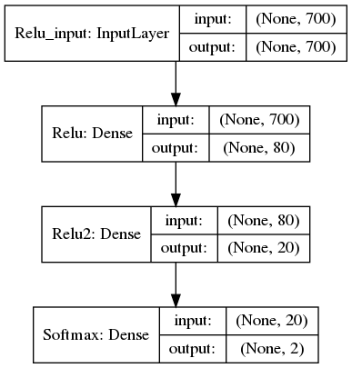
Figure 6: The Neural Network Classifier for the Scale invariant vs Conformally invariant three-point functions. It has 57,742 trainable parameters. It processes input data of 700 dimensional feature vectors $X$, which are passed to a fully connected layer of 80 relu-activated neurons, whose output feeds to a fully connected layer of 20 relu-activated neurons. The output of this layer is fed to a softmax layer which outputs two possible values for $Y$. ‘None’ is a placeholder to indicate that the neural network trains on an arbitrary number of training instances $(X,Y)$.

The takeaway from these computations seems to be that neural network classifiers can quite easily distinguish scale invariance from conformal invariance in the theory from the knowledge of the conformal dimensions or two point functions, as well as three point functions. It would be interesting to see if a similar classification is successful for spinning three-point correlation functions.

2.3 Crossing Symmetric Four-Point Functions

Given a four-point correlation function of identical scalar primary operators in a CFT

$$\left\langle\mathcal{O}_{1}\left(x_{1}\right)\mathcal{O}_{2}\left(x_{2}\right)\mathcal{O}_{3}\left(x_{4}\right)\mathcal{O}_{4}\left(x_{4}\right)\right\rangle\equiv f\left(x_{1},x_{2},x_{3},x_{4}\right)\,,$$ (5)

where we have again suppressed the dependence on conformal dimensions of the external operators, crossing symmetry is the property that:

$$f\left(x_{1},x_{2},x_{3},x_{4}\right)=f\left(x_{1},x_{3},x_{2},x_{4}\right)=f\left(x_{1},x_{4},x_{3},x_{2}\right)\,.$$ (6)

In the following we shall train a neural network classifier to recognize a four point function which is crossing symmetric, as opposed to a generic function of four variables which has no definite crossing symmetry property. Our overall strategy is the same as before. We will feed a data set of point clouds with and without this symmetry and train the neural network to distinguish between them. In practice, however, we achieve much better results by training the neural network to recognize the following expression

$$\begin{split}f\left(x_{1},x_{2},x_{3},x_{4}\right)&=f\left(x_{1}+\epsilon_{1},x_{3}+\epsilon_{3},x_{2}+\epsilon_{2},x_{4}+\epsilon_{4}\right)+\mathcal{O}\left(\epsilon\right)\\ &=f\left(x_{1}-\epsilon_{1},x_{4}-\epsilon_{4},x_{3}-\epsilon_{3},x_{2}-\epsilon_{2}\right)+\mathcal{O}\left(\epsilon\right)\,.\end{split}$$ (7)

Here $\epsilon_{i}$ may be viewed heuristically as a cutoff, whose role is not fully clear a priori. Its appearance indicates that for a neural network to recognize crossing symmetry, we need to study the crossing equation not just at the interchanged arguments, but in their neighbourhoods, the underlying reason for this is currently not obvious to us. In practice, we achieved good results by sampling point clouds of 100 points to define a training instance, and keeping $\epsilon\simeq 0.05$. The data set is enumerated in Table 6.

$\mathrm{Symmetry}$	$\mathrm{X}$	$\mathrm{Y}$
$\mathrm{Crossing\,\,Symmetric}$	$\big{(}\mathbf{x}_{1234},f^{(1234)},\mathbf{x}_{1324}+\epsilon,\,f^{(1234)}+\mathcal{O}(\epsilon)$, $\mathbf{x}_{1432}+\epsilon,\,f^{(1234)}+\mathcal{O}(\epsilon)\big{)}$	$\left(1,0\right)$
$\mathrm{Non-Symmetric}$	$\big{(}\mathbf{x}_{1234},f^{(1234)},\mathbf{x}_{1324}+\epsilon,\,f^{(1324)}+\epsilon$, $\mathbf{x}_{1432}+\epsilon,\,f^{(1423)}+\epsilon\big{)}$	$\left(0,1\right)$

Table 6: The training data for the recognition of crossing symmetric four-point functions. The neural network was trained on 1000 instances of this data, i.e. 500 crossing symmetric functions and 500 non-symmetric functions. $x_{ijkl}$ denotes the quadruplet $(x_{1},x_{j},x_{k},x_{l})$ and $f^{(ijkl)}$ denotes the value of the function $f$ sampled at the arguments $x_{ijkl}$.

The architecture of this classifier is sketched in Figure 7 and the learning curves are available in Figure 8.

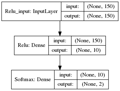
Figure 7: The Neural Network Classifier for recognizing crossing symmetry. This has 1532 trainable parameters.

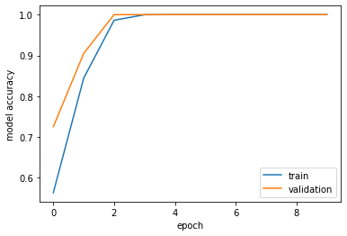
(a) Accuracy

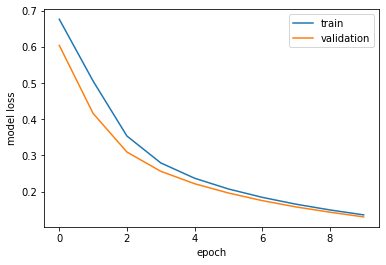
(b) Loss

Figure 8: The Accuracy and Loss curves for the crossing symmetry classification when the Neural Network in Figure 7 is fed the data in Table 6 with an 80/20 split for training and validation.

We have now seen that two important characteristics of CFT correlation functions, namely the conformal invariance of the three-point function and the crossing symmetry of the four-point function, can be recognized to great accuracy by neural networks. We shall next turn our attention to training the machine to recognize another characteristic of CFT four-point functions, i. e. their operator product expansion decomposition into individual conformal blocks.

3 Machine Learning The Conformal Block Expansion

In this section we shall consider some methods by which one may try to machine learn the conformal block expansion of a four-point function in a CFT. For definiteness and simplicity, we shall stick to an one-dimensional CFT, where the four-point function of identical scalar primary operator $\phi_{h_{\phi}}(x)$ may be decomposed as:

$$\langle\phi_{h_{\phi}}(x_{1})\phi_{h_{\phi}}(x_{2})\phi_{h_{\phi}}(x_{3})\phi_{h_{\phi}}(x_{4})\rangle=\frac{F_{\phi\phi\phi\phi}(z)}{|x_{12}|^{2h_{\phi}}|x_{34}|^{2h_{\phi}}}=\frac{\sum_{\{h\}}c_{h}\,z^{h}\,_{2}F_{1}\left(h,h,2h;z\right)}{|x_{12}|^{2h_{\phi}}|x_{34}|^{2h_{\phi}}}\,.$$ (8)

$$z=\frac{|x_{12}||x_{34}|}{|x_{13}||x_{24}|}.$$ (9)

The function $z^{h}\,_{2}F_{1}\left(h,h,2h;z\right)$ is the one-dimensional conformal block, which only depends on a single conformal cross ratio $z$ and is labeled by scaling dimension $h$ of the exchange operator $\mathcal{O}_{h}$, and $c_{h}$ is the associated OPE coefficient.

Given the expansion (8), two interesting questions naturally suggest themselves. Firstly, can neural networks be trained to detect the presence (or conversely the absence) of a conformal block belonging to a particular primary operator in the above expansion; and secondly, can machine be trained to estimate the value of the OPE coefficients $\{c_{h}\}$ for a given $F_{\phi\phi\phi\phi}(z)$. We shall provide supporting evidence for the affirmative answers to both questions. It is interesting to note that in the so-called “diagonal limit” where the conformal cross ratios $z=\bar{z}$ which is of interests for conformal bootstrap computations, the general d-dimensional conformal block can be expressed in a closed form in terms of a finite sum of generalized hypergeometric function ${}_{3}F_{2}$ Hogervorst:2013kva , we thus expect our analysis here can be readily adapted for more general situations . However we should also make a disclaimer here that we have merely regarded the conformal block as a complete kinematic basis, without imposing the additional consistency condition such as crossing symmetry, so this should only be taken as the first step towards using machine-learning method to perform conformal bootstrap.

3.1 A Warm-Up with the Fourier Expansion

We begin with an a priori simpler case of the Fourier decomposition in one dimension as a warm-up to the conformal block decomposition and demonstrate how various aspects of the Fourier expansion are machine-learnable. In particular, consider a function with a domain $x\in\left(-\frac{\pi}{2},\frac{\pi}{2}\right)$ that admits a purely sine expansion

$$f\left(x\right)=\sum_{n=1}^{\infty}a_{n}\,\sin\left(n\,x\right)\,.$$ (10)

We will train a neural network to answer the following two questions. Firstly, to identify a class of functions for which an arbitrary but fixed Fourier mode is missing in the expansion (10). Subsequently, we shall turn our attention to a harder regression problem, which is to have the neural network output the value of a fixed sine coefficient, given values of the function sampled in the interval $\left(-\frac{\pi}{2},\frac{\pi}{2}\right)$.

We should emphasize that the main goal of this computation is not to obtain a neural network implementation of the Fourier sine transform. Instead, we argue that by doing these classification and regression tasks accurately, we demonstrate neural networks are essentially able to identify fine-grained information about how symmetries manifest themselves in physical quantities. Both classes of functions that appear in Equation (11) carry the same $U(1)$ symmetry, and indeed the instances plotted in Figure 9 look roughly similar at first glance. But, to a neural network classifier, these functions are vastly different. This is further borne out by the Principal Component analysis that we will later present. The same sensitivity to the representations of symmetry that appear in the expansion of a function is also seen later in the context of the conformal block expansion. Highlighting this sensitivity is the main goal of this section.

For definiteness, we shall pick the $n=2$ mode for both the classification, and the regression tasks. Also, while a generic function $f(x)$ has an infinite number of sine modes, we shall consider a sub-class of functions for which $a_{n\geq 5}=0$. This is both because considering this sub-class is sufficient to illustrate the concepts that follow, and also because as we include higher and higher sine modes, the structure of the neural network required to accurately carry out these tasks becomes more and more complicated.

Beginning with the classification problem, we have two classes of functions, namely

$$f^{(1)}\left(x\right)=\sum_{n=1}^{4}a_{n}\,\sin\left(n\,x\right)\,,\qquad f^{(2)}\left(x\right)=\sum_{n=1,\,n\neq 2}^{4}a_{n}\,\sin\left(n\,x\right)\,.$$ (11)

We sample the function at 100 uniformly spaced points from $\left(-\frac{\pi}{2},\frac{\pi}{2}\right)$. The values of $f^{(1)}$ and $f^{(2)}$ at these points constitute the training data, as shown in Table 7.

$\mathrm{Modes}$	$\mathrm{X}$	$\mathrm{Y}$
$a_{n}\in(0,1)\,\forall\,n\leq 4$	$\left\{f^{(1)}\left(x_{i}\right)\quad|\quad x_{i}=-\frac{\pi}{2}+i\,\frac{\pi}{N}\,,i\in[0,N-1]\right\}$	$\left(1,0\right)$
$a_{2}=0$	$\left\{f^{(2)}\left(x_{i}\right)\quad|\quad x_{i}=-\frac{\pi}{2}+i\,\frac{\pi}{N}\,,i\in[0,N-1]\right\}$	$\left(0,1\right)$

Table 7: The training data for the classification of functions according to their Fourier sine modes. We took $N=100$, and $f^{(1)}$ and $f^{(2)}$ are as defined in (11). The neural network was trained on 200000 instances of this data, i.e. 100000 functions with all modes $a_{n\leq 4}$ randomly sampled from a normal distribution valued in $(0,1)$ and 100000 functions with the mode $a_{2}=0$ and the remaining modes sampled as before.

For illustration, we plot some functions of each class in Figure 9.

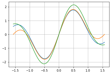
(a) Functions with $a_{n}\neq 0$.

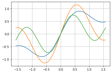
(b) Functions with $a_{2}=0$.

Figure 9: Functions expandable in terms of the first four sine modes. Different colors correspond to different functions.

From a visual inspection of the graphs, it does not seem very obvious that these functions fall into two sharply delineated categories, but as we see from the training curves in Figure 10(b) and 10(c), the neural network defined in Figure 10(a)

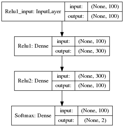
(a) The neural network architecture for the classifier.

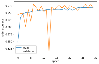
(b) Accuracy

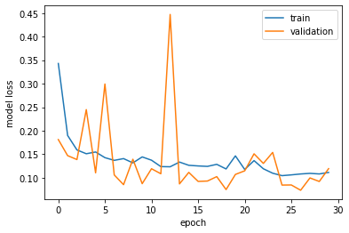
(c) Loss

Figure 10: Neural Network Classification of functions by their Fourier sine expansions. The 100 dimensional feature vector defined in Table 7 is fed to a two layers consisting of 300 and 100 relu-activated neurons respectively. The output is from the subsequent softmax layer.

is able to distinguish between the two classes to 97 percent accuracy by training over 30 epochs, which takes a few minutes on a laptop. We also observed that performance erodes rapidly as higher modes are turned on. We expect that this is a consequence of the Universal Approximation Theorem Cybenko1989 ; HORNIK1991251 , see also Chapter 4 of nielsenneural for a visual demonstration of the theorem. This essentially states that while it is certainly possible for a neural network to mimic a function with arbitrarily rich features, determining the necessary parameters of the network becomes an increasingly difficult task in practice.

We subsequently tested the classifier on 2000 new functions, 1000 of each class. The classifier distinguished them to 97 percent accuracy and the confusion matrix was $\big{(}\begin{smallmatrix}1000&0\\ 70&930\end{smallmatrix}\big{)}$, i.e. all 1000 instances of functions with vanishing $a_{2}$ were classified correctly, while 70 of the functions with all non-vanishing $a_{n}$ were mis-classified by the network, and 930 were correctly classified.

We now turn to the regression problem, i.e. given a function $f(x)$ with the sine expansion

$$f\left(x\right)=\sum_{n=1}^{4}a_{n}\,\sin\left(n\,x\right)\,,$$ (12)

we would like the neural network to output for us the coefficient $a_{2}$. The data set for the regression problem is outlined in Table 8.

$\mathrm{Modes}$	$\mathrm{X}$	$\mathrm{Y}$
$a_{n}\in(0,1)\,\forall\,n\leq 4$	$\left\{f\left(x_{i}\right)\right\}$	$\left\{a_{2}\sin\left(2\,x_{i}\right)\quad|\quad x_{i}=-\frac{\pi}{2}+i\,\frac{\pi}{4}\,,i\in[0,3]\right\}$

Table 8: The training data for learning the coefficient of the Fourier mode $a_{2}$ when supplied the function $f(x)$ defined in Equation (12). We choose $N=100$ and the $\left\{f(x_{i})\right\}$ are sampled at the $x_{i}$ defined previously in Table 7. The neural network was trained on 100000 instances of this data, i.e. 100000 functions with all modes $a_{n\leq 4}$ randomly sampled from a normal distribution valued in $(0,1)$.

Note that for the output $Y$, we have chosen to sample the mode $a_{2}\,\sin\left(2\,x_{i}\right)$ at four values of $x$, rather than directly output the value $a_{2}$. This is because the neural network is found to overfit to the training set when supplied with just the single value $a_{2}$. The architecture of the neural network is identical to the classifier in Figure 10(a), except that the softmax layer is replaced with a layer of four output neurons. Once the regressor is trained, we test it on new functions. Supplied with the four values of $a_{2}\,\sin\left(2\,x_{i}\right)$ as output from the regressor for each input $f(x)$, we divide them out by $\sin\left(2\,x_{i}\right)$ and take the median. This is our predicted value of $a_{2}$. We compare the predicted value with the actual value for 200 functions, and the result is given in Figure 11. We find that the regressor is able to predict the $a_{2}$ value to the accuracy within 0.5 percent. Though we do not show it here, similar results hold for the remaining modes.

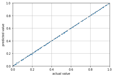
Figure 11: A comparison of the actual values of Fourier sine mode $a_{2}$ for 200 test functions with the corresponding predicted values. For a regressor working at 100 percent accuracy, the scatter points would lie precisely on the diagonal line $y=x$, shown as a dashed line here. We obtained an r-squared value of 0.9999.

3.2 The Conformal Block Expansion

With the experience of the Fourier sine expansion, let us now turn to the case of the one-dimensional conformal block expansion. Here we will make a simplifying assumption that the scaling dimensions $h$ of the operators being exchanged in the four point function (8) are integer valued . This assumption may seem somewhat non-physical, however this is sufficient for demonstrating that the presence or absence of a particular conformal block in the OPE expansion is machine learnable. Thus we start with the conformal block expansion:

$$\hat{F}_{\phi\phi\phi\phi}\left(z\right)=\sum_{n=0}^{\infty}c_{n}\,z^{n}\,_{2}F_{1}\left(n,n,2n;z\right)\,.$$ (13)

Furthermore as in the Fourier case, in practice, we truncate the sum over $n$ at a finite value $N$, which was 10 for classification and 5 for regression. Again, we pick the $n=2$ term for both classification, and regression. Curiously, the neural networks required to perform these tasks are much smaller than their counterparts for the Fourier case.

OPE Coefficients	$\mathrm{X}$	$\mathrm{Y}$
$c_{n}\in(0,1)\,\forall\,n\leq 10$	$\left\{f^{(1)}\left(x_{i}\right)\quad|\quad x_{i}=-0.8+i\,\frac{1.6}{N}\,,i\in[0,N-1]\right\}$	$\left(1,0\right)$
$c_{2}=0$	$\left\{f^{(2)}\left(x_{i}\right)\quad|\quad x_{i}=-0.8+i\,\frac{1.6}{N}\,,i\in[0,N-1]\right\}$	$\left(0,1\right)$

Table 9: The training data for the classification of functions (8) according to their non-vanishing OPE coefficients. We took $N=100$, and sampled the functions $f^{(1)}$ and $f^{(2)}$ defined in (14). The neural network was trained on 200000 instances of this data, i.e. 100000 functions with all modes $c_{n\leq 10}$ randomly sampled from a normal distribution valued in $(0,1)$ and 100000 functions with the mode $c_{2}=0$ and the remaining modes sampled as before.

We begin with the classification problem, where we have two classes of functions, i.e.

$$f^{(1)}\left(z\right)=\sum_{n=0}^{10}c_{n}\,z^{n}\,_{2}F_{1}\left(n,n,2n;z\right)\,,\qquad f^{(2)}\left(z\right)=\sum_{n=0,n\neq 2}^{10}c_{n}\,z^{n}\,_{2}F_{1}\left(n,n,2n;z\right)\,.$$ (14)

To build the training set, these functions were generated by randomly generating $c_{n}$s, normally distributed between 0 and 1. The functions were then sampled at 100 uniformly spaced points in the interval $(-0.8,0.8)$, again chosen for definiteness as the expressions are diverge at $|z|=1$, due to the presence of the hypergeometric function ${}_{2}F_{1}$ . Example functions of both classes are plotted in Figure 12, and the complete training data is described in Table 9.

(a) Functions with $c_{n}\neq 0$.

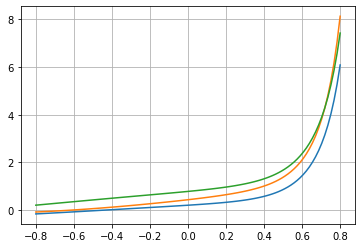
(b) Functions with $c_{2}=0$.

Figure 12: Instances of the two classes of functions enumerated in Equation (13). Different functions are represented by different colors.

As in the Fourier expansion case, there does not appear to be an obvious characteristic which separates the two classes. However, a neural network of a single layer of 40 relu activated neurons is able to distinguish the two classes to 96 percent accuracy. The training curves are shown in Figure 14 and the neural network architecture is shown in Figure 13.

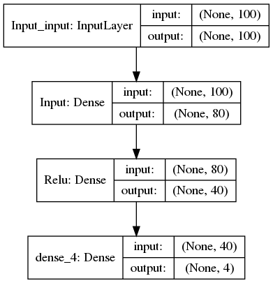
Figure 13: The neural network architecture used to perform classification and regression tasks for the conformal block expansion. The figure above corresponds to the regressor, which outputs the coefficient $c_{2}$ by giving values the quantity $c_{2}\,z^{2}\,{}_{2}F_{1}\left(2,2,4,z\right)$ at four different points $z$ at the output layer. The architecture of the classifier is identical, except that the output layer is now a softmax layer.

We subsequently tested this trained classifier on 2000 new functions, which it was able to distinguish again to 97 percent accuracy. The confusion matrix in this case was $\big{(}\begin{smallmatrix}1000&0\\ 67&933\end{smallmatrix}\big{)}$, i.e. all 1000 cases of the functions $f^{(2)}(z)$ were classified correctly, while 67 of the functions $f^{(1)}(z)$ were mis-classified as $f^{(2)}(z)$.

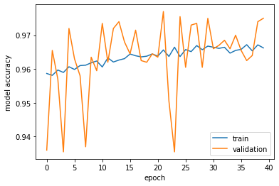
(a) Accuracy

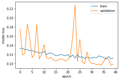
(b) Loss

Figure 14: Accuracy and Loss curves of the Neural Network classifier for the Conformal Block expansion.

We next turn to the regression problem for conformal blocks, which we pose as follows. Given a set of functions of the form

$$f\left(z\right)=\sum_{n=0}^{5}c_{n}\,z^{n}\,_{2}F_{1}\left(n,n,2n;z\right)\,,$$ (15)

we would like to train a neural network to predict the value of $c_{2}$. Our training data is described in Table 10.

OPE Coefficients	$\mathrm{X}$	$\mathrm{Y}$
$c_{n}\in(0,1)\,\forall\,n\leq 5$	$\left\{f\left(x_{i}\right)\right\}$	$\left\{c_{2}\,z^{2}\,_{2}F_{1}\left(2,2,4;z\right)\quad|\quad z\in\left\{-0.8,-0.4,0.4,0.8\,\right\}\,,\right\}$

Table 10: The training data for learning the OPE coefficient $c_{2}$ when supplied the function $f(x)$ defined in Equation (15). We choose $N=100$ and the $\left\{f(z_{i})\right\}$ are sampled at the $z_{i}$ defined previously in Table 9. The neural network was trained on 100000 instances of this data, i.e. 100000 functions with all modes $c_{n\leq 5}$ randomly sampled from a normal distribution valued in $(0,1)$. The final value of $c_{2}$ was extracted from the regressor by taking the median as described previously for the Fourier expansion.

As we saw for the classification example, the neural network architecture that is needed here turns out to be somewhat simpler than in the Fourier case discussed previously. In particular, it is a two layer network, consisting of 80 relu activated neurons in the first layer, and 40 relu activated neurons in the second layer. This network was trained for 50 epochs, and the comparison with actual values of $c_{2}$ and predicted values for 200 test functions is shown in Figure 15.

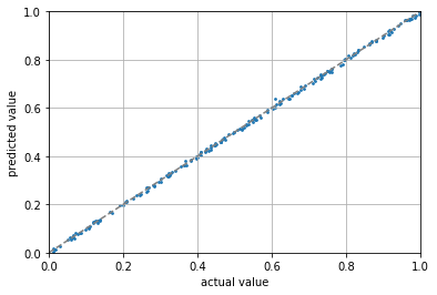
Figure 15: A comparison of the actual values of the OPE coefficient $c_{2}$ for 200 test functions with the corresponding predicted values. A regressor functioning at 100 percent accuracy would produce the dashed diagonal line corresponding to $y=x$ in the above graph. Actual results appear above as a scatter plot about that line. The r-squared value is 0.9988.

We again see that the neural network is able to predict the OPE coefficient $c_{2}$ appearing in the conformal block expansion of putative four-point functions to good accuracy.

3.3 Principal Components Analysis

The nature of this problems beckons for the distinction of a fundamental structure: since a simple neural network seems to tell whether a Fourier series or a conformal block expansion contains a particular term, is there an underlying difference between the respective graphs of the functions? We address this question first for the Fourier expansion and then for the conformal blocks. To do so, it is useful to think of the data in Table 7 in terms of point clouds in 100 dimensions as follows. If

$$X:=\left\{-\frac{\pi}{2}+j\frac{\pi}{100}\right\}_{j=0,\ldots,99}\,,$$ (16)

is a list of 100 real points, then Table 7 defines sets of point-clouds in $\mathbb{R}^{100}$: the functions $f^{(1)}(x)$ and $f^{(2)}(x)$ defined in (11) and evaluated at $X$ for random samples of coefficients $a_{n}$ drawn from a uniform distribution between $[0,1]$. Are these two data sets structurally different? Figure 9 might suggest a disparity and the neural network of Figure 10(a) does distinguish the two.

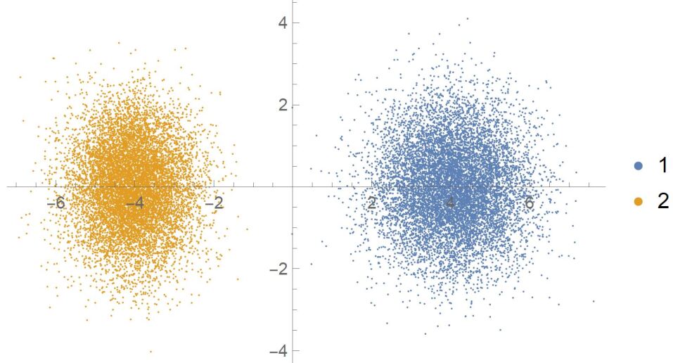
Figure 16: Principal component projections to 2-dimensions of the randomized 4-term Fourier expansions with and without the $\sin(2x)$ term. These functions are defined respectively as $f^{(1)}(x)$ and $f^{(2)}(x)$ in Equation (11). The functions $f^{(1)}(x)$ appear as a blue point cloud and $f^{(2)}(x)$ as a yellow point cloud.

Of course, 100-dimensions is not visualizable. Nevertheless, a standard technique lends itself. One can apply principal component analysis (PCA) where one can project down (while minimizing on the Euclidean distance to the lower dimension). We apply PCA and reduce to 2-dimensions for ease to the eye, and this is shown in Figure 16, with 1 (blue) and 2 (orange) marking $f^{(1)}$ and $f^{(2)}$ respectively. We see that the components are completely separated and thus indeed Fourier series with and without a particular term are different. One may similarly apply PCA on the conformal block classification problem of Section 3.2. The procedure is precisely the same as the Fourier case above. We then find that the datasets separate as per Figure 17 with the same color conventions as in the Figure 16.

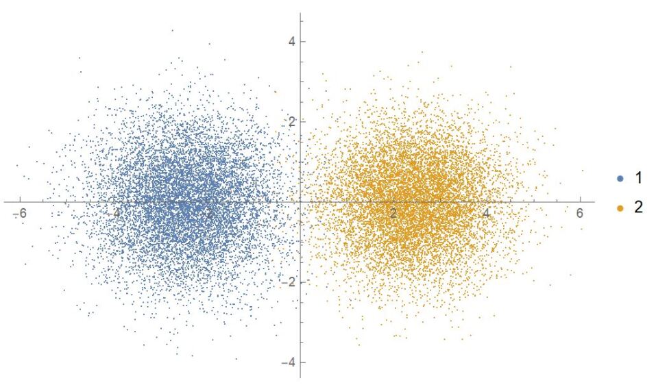
Figure 17: Principal component projections to 2-dimensions of the randomized conformal block expansions with and without the $c_{2}$ term. These functions are defined respectively as $f^{(1)}(z)$ and $f^{(2)}(z)$ in Equation (14). As before, $f^{(1)}(z)$s are represented by a blue point cloud and $f^{(2)}(z)$s by a yellow point cloud.

4 Neural Networks applied to the 3d Ising Model

In this section, we would like to use machine-learning to study the following questions. Firstly, we would like to train a neural network algorithm to classify operators in the 3d Ising Model based on their $\mathbb{Z}_{2}$ parity. This is a natural classification problem, along the lines of the ones addressed previously. Further, we shall investigate if it is possible to train a neural network on the existing spectral data Simmons-Duffin:2016wlq to estimate the conformal dimension of an operator given its spin by means of regression. We should emphasize that a key difference between conventional regression methods and neural network regression is that in conventional methods we fit a pre-selected curve, such as a straight line, or polynomial curve to the given data, while the neural network is simply fed the data and its usual hyper-parameters, and ‘decides’ the fitting curve on its own.

4.1 The 3d Ising Model CFT: Review

We now collect some relevant basic details about the 3d Ising Model, as well as a summary of our notations and conventions, referring the reader to the review Poland:2018epd for further details.

The 3d Ising model is a set of random spins $s_{i}=\pm 1$ in a cubic lattice in $\mathbb{R}^{3}$ with nearest neighbor interactions. The partition function is

$$\mathcal{Z}=\sum_{\{s_{i}\}}\exp\left(-J\sum_{\langle ij\rangle}s_{i}\cdot s_{i}\right)\,.$$ (17)

We note here that the lattice theory is invariant under the $\mathbb{Z}_{2}$ symmetry $s_{i}\mapsto-s_{i}$. It is well known that this model exhibits a phase transition, and at its critical point, conformal symmetry emerges and is described by a CFT, which is what we are interested in. We note here that neural networks have previously been trained to recognize this and other such phase transitions from random spin configurations generated by Monte-Carlo methods carrasquilla2017machine ; ch2017machine ; broecker2017machine ; JMLR:v18:17-527 ; d2020learning . Our interest is in the CFT occurring at this critical point. A useful microscopic realization of this CFT is in terms of a scalar field theory in three dimensions.

$$S=\int d^{3}x\,\left(\tfrac{1}{2}\left(\partial\sigma\right)^{2}+\tfrac{1}{2}\,m^{2}\sigma^{2}+\tfrac{1}{4!}\,\lambda\sigma^{4}\,\right)\,,$$ (18)

where both $m^{2}$ and $\lambda$ describe relevant couplings. At a critical value of the dimensionless ratio $m^{2}\over\lambda^{2}$, the long distance behavior of this model is described by the same CFT as the lattice model above.

Let us now turn to reviewing the physical data of the 3d Ising Model CFT as obtained by the bootstrap ElShowk:2012ht ; El-Showk:2014dwa ; Kos:2014bka ; Simmons-Duffin:2015qma ; Kos:2016ysd . The procedure adopted is to consider the four-point functions $\left\langle\sigma\sigma\sigma\sigma\right\rangle$, $\left\langle\epsilon\epsilon\epsilon\epsilon\right\rangle$, $\left\langle\sigma\sigma\epsilon\epsilon\right\rangle$ and the operator product expansions

$$\sigma\times\sigma=\sum_{\mathcal{O}}f_{\sigma\sigma\mathcal{O}}\,\mathcal{O}+\ldots\,,\quad\epsilon\times\epsilon=\sum_{\mathcal{O}}f_{\epsilon\epsilon\mathcal{O}}\,\mathcal{O}+\ldots\,,\quad\sigma\times\epsilon=\sum_{\mathcal{O}}f_{\sigma\epsilon\mathcal{O}}\,\mathcal{O}+\ldots\,,$$ (19)

where the ‘$\ldots$’ denote the contributions from the descendants. Requiring the unitarity and crossing symmetry for the above four-point functions constrains the conformal dimensions and OPE coefficients above. In particular as obtained in Kos:2016ysd :

$$\begin{split}\Delta_{\sigma}=0.5181489(10)\,,&\qquad f_{\sigma\sigma\epsilon}=1.0518537(41)\,,\\ \Delta_{\epsilon}=1.412625(10)\,,&\qquad f_{\epsilon\epsilon\epsilon}=1.532435(19)\,.\end{split}$$ (20)

The numerical and analytical results for the spectrum and the OPE coefficients of additional operators $\mathcal{O}$ required for crossing symmetry of these correlators were obtained in Simmons-Duffin:2016wlq for more than a hundred operators.

Here, we point out the existence of an important sub-class of operators known as double-twist operators Fitzpatrick:2012yx ; Komargodski:2012ek . It has been proven for a CFT in dimensions greater than two, and containing operators $\mathcal{O}_{1}$ and $\mathcal{O}_{2}$ of twist $\tau_{1}$ and $\tau_{2}$ that there exist infinite families of operators $[\mathcal{O}_{1}\mathcal{O}_{1}]_{n}$ of increasing spin and whose twist $\tau$ approaches $\tau_{1}+\tau_{2}+2n$ as for all integers $n\geq 0$. These played an important role in the analysis of Simmons-Duffin:2016wlq . We will shortly use the numerical results obtained there to train a neural network regressor to predict the twists of operators in the families $[\sigma\sigma]_{0}$ and $[\sigma\epsilon]_{0}$.

To sum up, the critical behavior of the 3d Ising model is described by a CFT with a $\mathbb{Z}_{2}$ global symmetry and two relevant scalars, $\sigma$, which is $\mathbb{Z}_{2}$-odd and $\epsilon$, which is $\mathbb{Z}_{2}$ even. Furthermore, physical data of the CFT, i.e. the conformal dimensions $\Delta_{\sigma}$ and $\Delta_{\epsilon}$ as well as the OPE coefficients $f_{\sigma\sigma\epsilon}$ and $f_{\epsilon\epsilon\epsilon}$ to lie in a tiny island by crossing symmetry of the scalar four-point function. Further, crossing symmetry also determines the conformal dimensions and OPE coefficients of operators appearing in the $\sigma\times\sigma$, $\sigma\times\epsilon$ and $\epsilon\times\epsilon$ operator product expansions (OPEs), though the precise evaluation of these numbers is a formidable numerical and analytical task Simmons-Duffin:2016wlq .

4.2 Learning The $\mathbb{Z}_{2}$ Symmetry of the 3d Ising Model

Consider the OPEs (19) of the 3d Ising Model. As $\sigma$ is $\mathbb{Z}_{2}$-odd and $\epsilon$ is $\mathbb{Z}_{2}$-even, the operators $\mathcal{O}$ appearing in the $\sigma\times\sigma$ and $\epsilon\times\epsilon$ OPEs are $\mathbb{Z}_{2}$ even, while the operators appearing in the $\sigma\times\epsilon$ OPE are $\mathbb{Z}_{2}$-odd. That is, a $\mathbb{Z}_{2}$-odd operator $\mathcal{O}$ has a strictly zero OPE coefficient $f_{\sigma\sigma\mathcal{O}}$ and $f_{\epsilon\epsilon\mathcal{O}}$, and a non-zero OPE coefficient $f_{\sigma\epsilon\mathcal{O}}$, while a $\mathbb{Z}_{2}$-even operator has a non-zero OPE coefficient for at least one of $f_{\sigma\sigma\mathcal{O}}$ and $f_{\epsilon\epsilon\mathcal{O}}$, and a strictly zero OPE coefficient $f_{\sigma\epsilon\mathcal{O}}$.

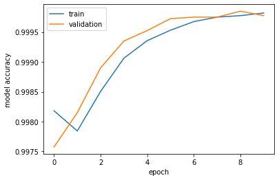
(a) Accuracy

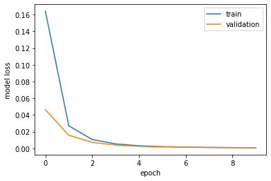
(b) Loss

Figure 18: The Accuracy and Loss curves for the $\mathbb{Z}_{2}$ classification Neural Network. The architecture of this network is outlined in Figure 19.

Here we shall train a neural network to classify operators that appear in the OPE of $\sigma\times\sigma$, $\sigma\times\epsilon$ and $\epsilon\times\epsilon$ under this $\mathbb{Z}_{2}$ symmetry. The training data for this classification is summarized in Table 11, and the architecture of the neural network classifier is shown in Figure 19. We achieved 99.85 percent accuracy by training for 10 epochs.

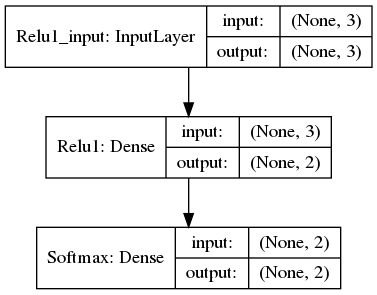
Figure 19: The Neural Network Classifier for classifying operators under a $\mathbb{Z}_{2}$ symmetry in a CFT. This has 68 trainable parameters.

$\mathbb{Z}_{2}$ charge	$\mathrm{f}_{\sigma\sigma\mathcal{O}}$	${f}_{\epsilon\epsilon\mathcal{O}}$	${f}_{\sigma\epsilon\mathcal{O}}$	$\mathrm{Y}$
$+1$	$x_{1}$	$x_{2}$	$0$	$\left(1,0\right)$
$-1$	0	0	$x_{3}$	$\left(0,1\right)$

Table 11: The training data for the classification of CFT operators $\mathcal{O}$ under a putative $\mathbb{Z}_{2}$ symmetry of the kind that appears in the 3d Ising Model. We continue to label the two fundamental fields of the CFT as $\sigma$ and $\epsilon$, and again $\sigma$ is taken to have $\mathbb{Z}_{2}$ charge $-1$ and $\epsilon$ is taken to have $\mathbb{Z}_{2}$ charge $+1$. The left-most column indicates the $\mathbb{Z}_{2}$ charge of $\mathcal{O}$ and is not part of the training data. The numerical values of the $x_{i}$s are randomly chosen positive real numbers between 0 and 1. We trained the classifier on on 100,000 instances of such data.

Having trained this classifier, we would like to examine how well it performs on the actual OPE data of the 3d Ising model obtained in Simmons-Duffin:2016wlq , see their Tables 1 to 7. Naively feeding this data to the classifier yields indifferent results. We believe that this was so because the OPE coefficients that appear in the 3d Ising model take numerical values ranging from $\mathcal{O}(1)$ to $\mathcal{O}(10^{-12})$ or so, while the classifier was trained on $\mathcal{O}(1)$ values. Indeed, once we transform the OPE data to take on positive values of order 1, via the function $f_{transformed}=|\log|f_{original}||$, we find that the classifier works to 100 percent accuracy with no mis-classifications .

4.3 Classifying higher rank discrete symmetries

It is also possible to carry out this classification with higher rank discrete symmetries. We consider a putative a CFT where there exist scalar fields $\varphi_{i}$ that carry a representation of $\mathbb{Z}_{3}$. We label the fields $\varphi_{0}$, $\varphi_{1}$ and $\varphi_{2}$, where the subscripts are the $\mathbb{Z}_{3}$ charges of the respective operators. Operator product expansions in this CFT would take the form

$$\begin{split}\varphi_{0}\times\varphi_{0}&=\sum_{\mathcal{O}_{(0)}}f_{0\,0\,\mathcal{O}_{(0)}}\,\mathcal{O}_{(0)}+\ldots\,,\qquad\varphi_{0}\times\varphi_{1}=\sum_{\mathcal{O}_{(1)}}f_{0\,1\,\mathcal{O}_{(1)}}\,\mathcal{O}_{(1)}+\ldots\,,\\ \varphi_{0}\times\varphi_{2}&=\sum_{\mathcal{O}_{(2)}}f_{0\,2\,\mathcal{O}_{(2)}}\,\mathcal{O}_{(2)+}+\ldots\,,\qquad\varphi_{1}\times\varphi_{2}=\sum_{\mathcal{O}_{(0)}}f_{1\,2\,\mathcal{O}_{(0)}}\,\mathcal{O}_{(0)}+\ldots\,,\end{split}$$ (21)

where as usual the ‘$\ldots$’ denotes the contributions from the descendants. The operator $\mathcal{O}_{(i)}$ has charge $i$ under the $\mathbb{Z}_{3}$ symmetry. Operators $\mathcal{O}_{(0)}$ would have generically non-zero OPE coefficients $f_{\varphi_{0}\,\varphi_{0}\,\mathcal{O}_{(0)}}$ and $f_{\varphi_{1}\,\varphi_{2}\,\mathcal{O}_{(0)}}$, operators $\mathcal{O}_{(1)}$ would have a non-zero $f_{\varphi_{0}\,\varphi_{0}\,\mathcal{O}_{(1)}}$ and lastly, operators $\mathcal{O}_{(2)}$ would have generically non-zero OPE coefficients $f_{\varphi_{1},\varphi_{1}\,\mathcal{O}_{(2)}}$ and $f_{\varphi_{0}\,\varphi_{0}\,\mathcal{O}_{(2)}}$ respectively. All other OPE coefficients would be zero on account of the $\mathbb{Z}_{3}$ symmetry.

We generated the data representing these features as per Table 12, and trained the neural network classifier described in Figure 20 on it.

$\mathbb{Z}_{3}$ charge	$\mathrm{f}_{\varphi_{0}\varphi_{0}\mathcal{O}}$	${f}_{\varphi_{0}\varphi_{1}\mathcal{O}}$	${f}_{\varphi_{0}\varphi_{2}\mathcal{O}}$	${f}_{\varphi_{1}\varphi_{1}\mathcal{O}}$	${f}_{\varphi_{1}\varphi_{2}\mathcal{O}}$	$\mathrm{Y}$
$0$	$x_{1}$	$0$	$0$	0	$x_{2}$	$\left(1,0,0\right)$
$1$	0	$x_{3}$	0	0	0	$\left(0,1,0\right)$
$2$	0	0	$x_{4}$	$x_{5}$	0	$\left(0,0,1\right)$

Table 12: The training data for the classification of CFT operators $\mathcal{O}$ under a putative $\mathbb{Z}_{3}$ symmetry of the kind defined in Equation 21. The left-most column indicates the $\mathbb{Z}_{3}$ charge of $\mathcal{O}$ and is not part of the training data. The numerical values of the $x_{i}$s are randomly chosen positive real numbers between 0 and 1. We trained the classifier on on 100,000 instances of such data.

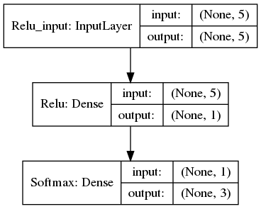
Figure 20: The Neural Network Classifier for classifying operators under a $\mathbb{Z}_{3}$ symmetry in a CFT. This has 12 trainable parameters.

The accuracy and loss curves during training are shown in Figure 21. We could train to 99.78 percent accuracy over 10 epochs. We also tested the classifier on 2000 instances of freshly generated putative OPE data of the kind detailed in Table 12, which it had not been trained on. It could classify those data to 99.73 percent accuracy.

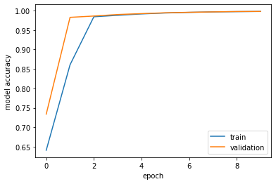
(a) Accuracy

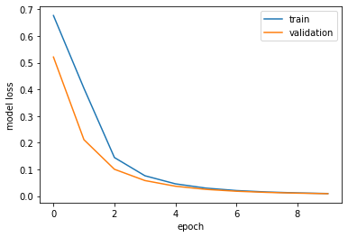
(b) Loss

Figure 21: The Accuracy and Loss curves for the $\mathbb{Z}_{3}$ Classification.

We note here that it should be possible to similarly consider higher-rank symmetry groups like $\mathbb{Z}_{4}$ and $\mathbb{Z}_{2}\times\mathbb{Z}_{2}$ and especially $\mathrm{S}_{N}\times\mathbb{Z}_{2}$ and try to train neural network classifiers to recognize these symmetries from the OPE coefficients. The CFTs with such discrete symmetries have been studied via conformal bootstrap in Rong:2017cow and Stergiou:2018gjj . It would be interesting to examine if the operators there can be similarly classified under their respective discrete symmetries by these ML methods.

4.4 Learning the Spectrum of the 3d Ising Model

Having examined the performance of neural networks on various classification tasks, we now turn to regression tasks. In particular, we shall train a neural network on the available spectral data of the 3d Ising model obtained in Simmons-Duffin:2016wlq by combining numerical and analytical bootstrap methods to learn the twist of the exchange operator as a function of its spin. We shall also further specialize to the OPE families $[\sigma\sigma]_{0}$ and $[\sigma\epsilon]_{0}$. The fitting data for these operators are taken from Tables 3 and 6 of Simmons-Duffin:2016wlq . We remind the reader that these tables give the data for the quantum numbers $\tau$ and $\ell$, which are related to $\bar{h}$ via

$$\bar{h}=\frac{\tau}{2}+\ell\,.$$ (22)

Also, the twists of operators of even spin and odd spin fall into two different curves in the $[\sigma\epsilon]_{0}$ family. It is interesting to note at this point that the three curves can also be fit almost exactly with a judicious choice of fitting ansatz. In particular, we consider the functions

$$\begin{split}\tau_{1}\left(\bar{h}\right)&=\tanh\left(a_{1}\,\bar{h}+b_{1}\right)+\tanh\left(a_{2}\,\bar{h}+b_{2}\right)+c\,,\\ \tau_{2}\left(\bar{h}\right)&=\frac{p}{\tanh\left(q_{1}\,\bar{h}+r_{1}\right)-\tanh\left(q_{2}\,\bar{h}+r_{2}\right)}+s\,.\end{split}$$ (23)

The data for $\tau_{[\sigma\sigma]_{(0)}}$ turns out to fit to $\tau_{1}$ with the parameters

$$a_{1}=0.0740199\,,\,b_{1}=2.42646\,,\,a_{2}=0.3991\,,\,b_{2}=1.18916\,,\,c=-0.964377\,,$$ (24)

with R-squared $1.0$ and total (corrected) squared error less than $0.001$. Likewise, the data for odd spin operators in the $[\sigma\sigma]_{(0)}$ family fits to $\tau_{1}$ with the parameters

$$a_{1}=0.0349198\,,\,b_{1}=1.18396\,,\,a_{2}=0.203412\,,\,b_{2}=0.706744\,,\,c=-0.129985\,,$$ (25)

while the odd spin operators fit to $\tau_{2}$ with the parameters

$$\begin{split}p&=0.024275\,,\,q_{1}=0.0767471\,,\,r_{1}=1.13926\,,\\ q_{2}&=-0.0242292\,,\,r_{2}=1.09043\,,s=1.96356\,,\end{split}$$ (26)

also with R-squared around $1.0$. The corresponding regression curves are plotted in Figure 22. It is perhaps curious that the relatively simple functional forms of Equation (23) seem to effectively capture the much more complicated expressions obtained through direct analytical methods Simmons-Duffin:2016wlq , and it may be interesting to understand this further.

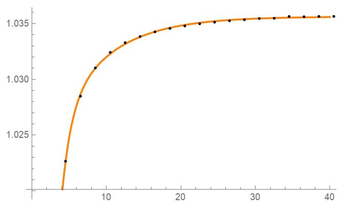
(a) Regression for $\tau_{[\sigma\epsilon]_{0}}$

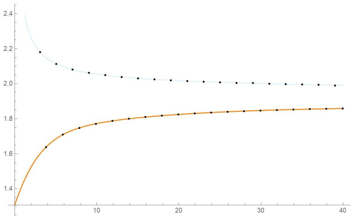
(b) Regression for $\tau_{[\sigma\sigma]_{0}}$

Figure 22: Directly fitting a functional form to the 3d Ising data. We see that a judicious but somewhat non-obvious choice of fitting functions (23) leads to an impressive fit with the available data.

For the moment, we will simply note that the success of this ansatz also suggests that we may try training a neural network on this data with $\tanh$ activation functions. We find that the size of the network required to produce comparable results is dramatically smaller than when choosing say sigmoid or relu activation functions, reducing to a layer of 15 neurons followed by a second hidden layer of 10 neurons. This network is displayed in Figure 23.

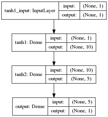
Figure 23: The Neural Network Regressor for predicting operator twists in the $[\sigma\sigma]_{0}$ and $[\sigma\epsilon]_{0}$ families in the 3d Ising Model. This has 81 trainable parameters and is run for 6000 epochs. The corresponding regression curves appear in Figure

Further, when supplying the data to the neural network for fitting, we found that performance improved when the data was fed in the form

$$\left(X,Y\right)\qquad:\qquad\left(\bar{h}^{-1},\tau\right)\,,$$ (27)

for $\tau_{[\sigma\sigma]_{0}}$ regression and

$$\left(X,Y\right)\qquad:\qquad\left(\bar{h}^{-2},\tau\right)\,,$$ (28)

for $\tau_{[\sigma\epsilon]_{0}}$ regression. The training of the regressor was significantly more stable when the data was fed in this form. The regression curves obtained after training for six thousand epochs are shown in Figure 24, along with their extrapolations to $\bar{h}=70$.

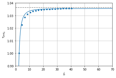
(a) Regression for $\tau_{[\sigma\sigma]_{0}}$

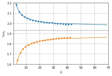
(b) Regression for $\tau_{[\sigma\epsilon]_{0}}$

Figure 24: Neural Network Regression for the 3d Ising Model spectrum. The smooth lines are the regression curves, the points are the numerical values obtained in Simmons-Duffin:2016wlq without the error bars. The dotted line in (a) denotes the asymptotic value $\tau=2\Delta_{\sigma}$, while the dotted line in (b) denotes the asymptotic value $\tau=\Delta_{\sigma}+\Delta_{\epsilon}$. The curves are extrapolated out to $\bar{h}=70$. The r-squared coefficient for (a) is 0.9804, and for (b) is 0.9966 for the even spin operators (blue line) and 0.9926 for the odd spin operators (orange line).

Before we close this section we would like to make a few comments about the choice of activation function. We have remarked previously that an important feature of ML based regression methods is that we do not feed the network with a trial form of the function to fit to. Why, then, is the architecture of the regressor so sensitive to the choice of activation function? Or at least, the architecture seems indifferent to choosing between relu and sigmoid activations but simplifies dramatically when the tanh activation function is chosen. We believe that at least some insight might be gained from the fitting functions in Equation (23). These suggest that the tanh functions are a particularly nice basis choice to expand these curves in, and the choice of activation function is at least intuitively a choice of basis functions to expand the neural network decision function in. A ‘good’ basis would have fewer undetermined coefficients, and this is what we seem to have found somewhat serendipitously with our choice of tanh as the activation function.

Appendices

In these appendices, we briefly summarize some rudiments on neural networks and principal components which are used in the text.

Appendix A Neural Networks

In this section, we provide a quick introduction to neural networks. This section is far from an exhaustive review on the working of neural networks, we only aim to lay down the relevant terms and a few notations. Neural networks are extremely useful for performing machine learning tasks such as classification and regression. A typical neural network consists of neurons also referred to as the single layer perceptron (SLP), arranged in layers on top of each other. Each such neuron is for all practical purposes a function of a vector valued input $z$, with components $z_{i}$ and is arranged to have in it real valued parameters $\omega_{i}$ called weights and $b$ called the bias. Thus, an SLP is a function of the form $f(\sum_{i}\omega_{i}x_{i}^{j}+b)$. Where $x_{i}^{j}$ is the $i$th component of the $j$th input. The function $f(z)$ familiar to neural network practitioners as the activation function is often taken to be a sigmoid,

$$f(z)=\sigma(z)=\frac{1}{1+exp(-z)}\,,$$ (29)

though other choices such as $f(z)=\tanh(z)$ and the rectifier function

$$f(z)=\max\left(0,z\right)\,,$$ (30)

are also equally popular. A neuron activated by the rectifier function is known as a rectifier linear unit, or a relu. We have used relus almost as a de facto choice in our neural networks above.

The process of training a neural network is then to find appropriate values for the weights $w_{i}$ and biases $b$ such that the desired goal is achieved. This is illustrated by the following example, suppose we are to perform a classification task using neural networks and we are supplied with a labeled dataset of the form D $=\{x_{i}^{j},d^{j}\}$, where $x_{i}$ is some vector belonging to a class specified by the labels $d^{j}$. The task is to train a neural network to accurately predict the class label of an instance not contained in D. This task can be achieved in two steps, first by specifying what is known to the neural network practitioners as the loss function. For classification tasks a typical loss function is the following,

$$f_{loss}=\sum_{j}(f(\omega_{i}x_{i}^{j}+b)-d^{j})^{2}.$$ (31)

The second step is to optimize the loss function over the parameters $w_{i}$ and $b$ using algorithms such as the Stochastic gradient descent. The performance of a neural network after training is evaluated on a part of the dataset D set aside before training. This is known as the test data, while D modulo test data $=$ training data. The performance of a neural network is evaluated with respect to some metric, typically in a classification task, the metric is accuracy. Thus the essentials associated to a neural network are, The training data, the test data, the activation functions, the loss function and the optimization algorithm.

Appendix B Principal Component Analysis (PCA)

In this section we briefly introduce the principal component analysis technique, which is employed for creating a low dimensional representation for a very high dimensional dataset. Again, we do not attempt an exhaustive review. We will give a brief illustration of a situation where PCA might come handy.

Suppose we are given a dataset D $\{x_{i}^{j},d^{j}\}$ for a classification task. Let’s say that the vectors $x^{j}$ belong to a very high dimensional space of dimensionality $n$ and it may be desirable to use low dimensional projections of $x^{j}$s for performing the classification. However the projections must be such that information from all the original features is retained. This is precisely what PCA achieves. This is done by defining new variables or features $y_{i}^{j}$ such that,

$$y_{i}^{j}=f_{i}^{j}(x_{1},x_{2},\cdots,x_{n}).$$ (32)

These new variables called principal components are chosen such that they are orthogonal to each other. After the principal components are defined, dimensionality reduction is achieved by keeping only those components which are of most relevance, the relevance being often measured by the variance explained.

References

- (1) A. M. Polyakov, Fermi-Bose Transmutations Induced by Gauge Fields, Mod. Phys. Lett. A 3 (1988) 325.
- (2) N. Shaji, R. Shankar and M. Sivakumar, On Bose-fermi Equivalence in a U(1) Gauge Theory With Chern-Simons Action, Mod. Phys. Lett. A 5 (1990) 593.
- (3) E. H. Fradkin and F. A. Schaposnik, The Fermion - boson mapping in three-dimensional quantum field theory, Phys. Lett. B 338 (1994) 253 [hep-th/9407182].
- (4) S. Giombi, S. Minwalla, S. Prakash, S. P. Trivedi, S. R. Wadia and X. Yin, Chern-Simons Theory with Vector Fermion Matter, Eur. Phys. J. C 72 (2012) 2112 [1110.4386].
- (5) O. Aharony, G. Gur-Ari and R. Yacoby, d=3 Bosonic Vector Models Coupled to Chern-Simons Gauge Theories, JHEP 03 (2012) 037 [1110.4382].
- (6) O. Aharony, G. Gur-Ari and R. Yacoby, Correlation Functions of Large N Chern-Simons-Matter Theories and Bosonization in Three Dimensions, JHEP 12 (2012) 028 [1207.4593].
- (7) I. Klebanov and A. Polyakov, AdS dual of the critical O(N) vector model, Phys. Lett. B 550 (2002) 213 [hep-th/0210114].
- (8) E. Sezgin and P. Sundell, Massless higher spins and holography, Nucl. Phys. B 644 (2002) 303 [hep-th/0205131].
- (9) M. R. Gaberdiel and R. Gopakumar, An AdS_3 Dual for Minimal Model CFTs, Phys. Rev. D 83 (2011) 066007 [1011.2986].
- (10) M. Beccaria and A. A. Tseytlin, Vectorial AdS5/CFT4 duality for spin-one boundary theory, J. Phys. A 47 (2014) 492001 [1410.4457].
- (11) J.-B. Bae, E. Joung and S. Lal, On the Holography of Free Yang-Mills, JHEP 10 (2016) 074 [1607.07651].
- (12) S. Rychkov, Conformal Bootstrap in Three Dimensions?, 1111.2115.
- (13) S. El-Showk, M. F. Paulos, D. Poland, S. Rychkov, D. Simmons-Duffin and A. Vichi, Solving the 3D Ising Model with the Conformal Bootstrap, Phys. Rev. D 86 (2012) 025022 [1203.6064].
- (14) S. El-Showk, M. F. Paulos, D. Poland, S. Rychkov, D. Simmons-Duffin and A. Vichi, Solving the 3d Ising Model with the Conformal Bootstrap II. c-Minimization and Precise Critical Exponents, J. Stat. Phys. 157 (2014) 869 [1403.4545].
- (15) F. Kos, D. Poland, D. Simmons-Duffin and A. Vichi, Precision Islands in the Ising and Models, JHEP 08 (2016) 036 [1603.04436].
- (16) D. Simmons-Duffin, The Lightcone Bootstrap and the Spectrum of the 3d Ising CFT, JHEP 03 (2017) 086 [1612.08471].
- (17) S. M. Chester, W. Landry, J. Liu, D. Poland, D. Simmons-Duffin, N. Su et al., Carving out OPE space and precise model critical exponents, 1912.03324.
- (18) J. Rong and N. Su, Scalar CFTs and Their Large N Limits, JHEP 09 (2018) 103 [1712.00985].
- (19) A. Stergiou, Bootstrapping hypercubic and hypertetrahedral theories in three dimensions, JHEP 05 (2018) 035 [1801.07127].
- (20) C. Beem, M. Lemos, P. Liendo, L. Rastelli and B. C. van Rees, The superconformal bootstrap, JHEP 03 (2016) 183 [1412.7541].
- (21) C. Beem, M. Lemos, L. Rastelli and B. C. van Rees, The (2, 0) superconformal bootstrap, Phys. Rev. D 93 (2016) 025016 [1507.05637].
- (22) L. F. Alday, Large Spin Perturbation Theory for Conformal Field Theories, Phys. Rev. Lett. 119 (2017) 111601 [1611.01500].
- (23) R. Gopakumar, A. Kaviraj, K. Sen and A. Sinha, A Mellin space approach to the conformal bootstrap, JHEP 05 (2017) 027 [1611.08407].
- (24) L. F. Alday, J. Henriksson and M. van Loon, Taming the -expansion with large spin perturbation theory, JHEP 07 (2018) 131 [1712.02314].
- (25) O. Aharony, L. F. Alday, A. Bissi and R. Yacoby, The Analytic Bootstrap for Large Chern-Simons Vector Models, JHEP 08 (2018) 166 [1805.04377].
- (26) Y.-H. He, Deep-Learning the Landscape, 1706.02714.
- (27) Y.-H. He, Machine-learning the string landscape, Phys. Lett. B 774 (2017) 564.
- (28) D. Krefl and R.-K. Seong, Machine Learning of Calabi-Yau Volumes, Phys. Rev. D 96 (2017) 066014 [1706.03346].
- (29) F. Ruehle, Evolving neural networks with genetic algorithms to study the String Landscape, JHEP 08 (2017) 038 [1706.07024].
- (30) J. Carifio, J. Halverson, D. Krioukov and B. D. Nelson, Machine Learning in the String Landscape, JHEP 09 (2017) 157 [1707.00655].
- (31) H. Erbin and S. Krippendorf, GANs for generating EFT models, 1809.02612.
- (32) K. Hashimoto, S. Sugishita, A. Tanaka and A. Tomiya, Deep learning and the AdS/CFT correspondence, Phys. Rev. D 98 (2018) 046019 [1802.08313].
- (33) Y.-H. He, The Calabi-Yau Landscape: from Geometry, to Physics, to Machine-Learning, 1812.02893.
- (34) F. Ruehle, Data science applications to string theory, Physics Reports 839 (2020) 1 .
- (35) I. M. Comsa, M. Firsching and T. Fischbacher, SO(8) Supergravity and the Magic of Machine Learning, JHEP 08 (2019) 057 [1906.00207].
- (36) C. Krishnan, V. Mohan and S. Ray, Machine Learning Gauged Supergravity, Fortsch. Phys. 68 (2020) 2000027 [2002.12927].
- (37) M. Chernodub, H. Erbin, I. Grishmanovskii, V. Goy and A. Molochkov, Casimir effect with machine learning, 1911.07571.
- (38) M. Chernodub, H. Erbin, V. Goy and A. Molochkov, Topological defects and confinement with machine learning: the case of monopoles in compact electrodynamics, 2006.09113.
- (39) P. Betzler and S. Krippendorf, Connecting Dualities and Machine Learning, Fortsch. Phys. 68 (2020) 2000022 [2002.05169].
- (40) J. Bao, S. Franco, Y.-H. He, E. Hirst, G. Musiker and Y. Xiao, Quiver Mutations, Seiberg Duality and Machine Learning, 2006.10783.
- (41) Y.-H. He, E. Hirst and T. Peterken, Machine-Learning Dessins d’Enfants: Explorations via Modular and Seiberg-Witten Curves, 2004.05218.
- (42) D. Simmons-Duffin, A Semidefinite Program Solver for the Conformal Bootstrap, JHEP 06 (2015) 174 [1502.02033].
- (43) W. Landry and D. Simmons-Duffin, Scaling the semidefinite program solver SDPB, 1909.09745.
- (44) D. Poland, S. Rychkov and A. Vichi, The Conformal Bootstrap: Theory, Numerical Techniques, and Applications, Rev. Mod. Phys. 91 (2019) 015002 [1805.04405].
- (45) A. Ashmore, Y.-H. He and B. A. Ovrut, Machine learning Calabi-Yau metrics, 1910.08605.
- (46) P. Mehta, M. Bukov, C.-H. Wang, A. G. Day, C. Richardson, C. K. Fisher et al., A high-bias, low-variance introduction to machine learning for physicists, Physics Reports 810 (2019) 1 .
- (47) J. Bao, Y.-H. He, E. Hirst and S. Pietromonaco, Lectures on the Calabi-Yau Landscape, 2001.01212.
- (48) J. Sirignano and K. Spiliopoulos, Dgm: A deep learning algorithm for solving partial differential equations, Journal of Computational Physics 375 (2018) 1339.
- (49) M. L. Piscopo, M. Spannowsky and P. Waite, Solving differential equations with neural networks: Applications to the calculation of cosmological phase transitions, Phys. Rev. D 100 (2019) 016002 [1902.05563].
- (50) P. Broecker, J. Carrasquilla, R. G. Melko and S. Trebst, Machine learning quantum phases of matter beyond the fermion sign problem, Scientific reports 7 (2017) 1.
- (51) S. Krippendorf and M. Syvaeri, Detecting Symmetries with Neural Networks, 2003.13679.
- (52) Y. Lecun, L. Bottou, Y. Bengio and P. Haffner, Gradient-based learning applied to document recognition, Proceedings of the IEEE 86 (1998) 2278.
- (53) A. Krizhevsky, I. Sutskever and G. E. Hinton, Imagenet classification with deep convolutional neural networks, in Proceedings of the 25th International Conference on Neural Information Processing Systems - Volume 1, NIPS’12, (Red Hook, NY, USA), p. 1097–1105, Curran Associates Inc., 2012.
- (54) L. Alessandretti, A. Baronchelli and Y.-H. He, Machine Learning meets Number Theory: The Data Science of Birch-Swinnerton-Dyer, 1911.02008.
- (55) Y.-H. He and M. Kim, Learning Algebraic Structures: Preliminary Investigations, 1905.02263.
- (56) Y. Nakayama, Scale invariance vs conformal invariance, Phys. Rept. 569 (2015) 1 [1302.0884].
- (57) M. Hogervorst, H. Osborn and S. Rychkov, Diagonal Limit for Conformal Blocks in Dimensions, JHEP 08 (2013) 014 [1305.1321].
- (58) H.-Y. Chen and H. Kyono, On conformal blocks, crossing kernels and multi-variable hypergeometric functions, JHEP 10 (2019) 149 [1906.03135].
- (59) G. Cybenko, Approximation by superpositions of a sigmoidal function, Mathematics of Control, Signals and Systems 2 (1989) 303.
- (60) K. Hornik, Approximation capabilities of multilayer feedforward networks, Neural Networks 4 (1991) 251 .
- (61) M. A. Nielsen, Neural networks and deep learning, 2018.
- (62) A. Geron, Hands-on machine learning with Scikit-Learn and TensorFlow :. O’Reilly,, Beijing, first edition. ed., 2017.
- (63) Y. LeCun and C. Cortes, MNIST handwritten digit database, .
- (64) J. Carrasquilla and R. G. Melko, Machine learning phases of matter, Nature Physics 13 (2017) 431.
- (65) K. Ch’Ng, J. Carrasquilla, R. G. Melko and E. Khatami, Machine learning phases of strongly correlated fermions, Physical Review X 7 (2017) 031038.
- (66) A. Morningstar and R. G. Melko, Deep learning the ising model near criticality, Journal of Machine Learning Research 18 (2018) 1.
- (67) F. D’Angelo and L. Böttcher, Learning the ising model with generative neural networks, Physical Review Research 2 (2020) 023266.
- (68) F. Kos, D. Poland and D. Simmons-Duffin, Bootstrapping Mixed Correlators in the 3D Ising Model, JHEP 11 (2014) 109 [1406.4858].
- (69) A. Fitzpatrick, J. Kaplan, D. Poland and D. Simmons-Duffin, The Analytic Bootstrap and AdS Superhorizon Locality, JHEP 12 (2013) 004 [1212.3616].
- (70) Z. Komargodski and A. Zhiboedov, Convexity and Liberation at Large Spin, JHEP 11 (2013) 140 [1212.4103].