Predicting Length of Stay in the Intensive Care Unit with
Temporal Pointwise Convolutional Networks

Abstract

We present a new deep learning architecture based on the combination of temporal convolution and pointwise (1x1) convolution to predict length of stay on the eICU critical care dataset. The model – which we refer to as Temporal Pointwise Convolution (TPC) – is specifically designed to mitigate for common challenges with Electronic Health Records (EHRs), such as skewness, irregular sampling and missing data. In doing so, we have achieved significant performance benefits of 18-51% (metric dependent) over the commonly used Long-Short Term Memory (LSTM) network, and the Transformer, a multi-head self-attention network.

1 Introduction

In-patient length of stay (LoS) is strongly associated with inflated hospital costs (Rapoport et al., 2003) and the risk of hospital acquired infection and mortality (Hassan et al., 2010; Laupland et al., 2006). Improved hospital bed planning has the potential to reduce these risks (Blom et al., 2015). However, this relies on accurate discharge date estimates.

We propose a new deep learning architecture to improve automatic LoS prediction. Like in Harutyunyan et al. (2019), we predict the remaining LoS of patients in the ICU. Our model combines the strengths of Temporal Convolutional Layers (van den Oord et al., 2016; Kalchbrenner et al., 2016) in capturing causal dependencies across time, and Pointwise Convolutional Layers (Lin et al., 2013) in computing higher level features from interactions in the feature domain. We show that these methods complement each other by extracting different information. Our model outperforms the commonly used Long-Short Term Memory (LSTM) network (Hochreiter and Schmidhuber, 1997) and the Transformer (Vaswani et al., 2017).

We also make a case for using the mean squared logarithmic error (MSLE) loss function to train LoS models, as it helps to mitigate for positive skew in the LoS. Our code is available at: https://github.com/EmmaRocheteau/eICU-LoS-prediction.

2 Related Work

LSTMs have been by far the most popular model for predicting LoS and have achieved state-of-the-art results (Harutyunyan et al., 2019; Sheikhalishahi et al., 2019; Rajkomar et al., 2018). They have also been applied to other patient prediction tasks e.g. forecasting diagnoses and medications (Choi et al., 2015; Lipton et al., 2015), and mortality prediction (Che et al., 2018; Harutyunyan et al., 2019; Shickel et al., 2019). More recently, the Transformer model (Vaswani et al., 2017) – which was originally designed for natural language processing (NLP) – has marginally outperformed the LSTM on the LoS task (Song et al., 2018). Therefore, the LSTM and the Transformer were chosen as key baselines.

3 Methods

We design our model to extract both trends and inter-feature relationships. Clinicians do this when assessing their patients e.g. they might check how the respiratory rate is changing over time, and they may also look at combination features e.g. the PaO₂/FiO₂ ratio.

Temporal Convolution

Temporal Convolution Networks (TCNs) (van den Oord et al., 2016; Kalchbrenner et al., 2016) are models that convolve over the time dimension. We use stacked TCNs to extract temporal trends in our data. Unlike most implementations, we do not share weights across features i.e. weight sharing is only across time (like in Xception (Chollet, 2016)). This is because our features differ sufficiently in their temporal characteristics to warrant specialised processing. In TCNs, the receptive field sizes are highly adaptable. They can be increased by using greater dilation, larger kernel sizes or by stacking more layers. By contrast, RNNs can only process one time step at a time.

Pointwise Convolution

Pointwise (or 1x1) convolution (Lin et al., 2013) is typically used to reduce the dimensions in an input (Szegedy et al., 2014). However we use it to compute interaction features from the existing feature set at each timepoint.

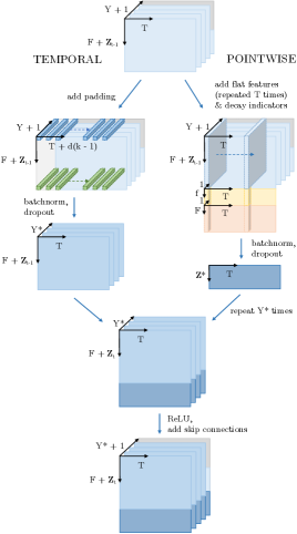
Figure 1: One layer of the TPC model. F is the number of time series features. T is the time series length. Y is the number of temporal channels per feature in the previous TPC layer (except for the first layer where Y is 1; decay indicators (explained under ‘Time Series’ in A.4) make up this channel). Z_t-1 is the cumulative number of pointwise outputs from all previous TPC layers. Y^∗ and Z^∗ are the number of temporal channels per feature and pointwise outputs respectively in the current TPC layer. Z${}_{t}=$ Z${}_{t-1}+$ Z^∗. The differently coloured temporal filters indicate independent parameters. $d$ is the temporal dilation, $k$ is the kernel size. Decay indicator features (A.4) are shown in orange, $f$ flat features are shown in yellow. The skip connections consist of F original features (grey) and Z_t+1 pointwise outputs (light blue). We ignore the batch dimension for clarity.

Skip Connections

We propagate skip connections (He et al., 2015) which allow each layer to see the original data and the pointwise outputs from previous layers. This helps the network to cope with infrequently sampled data (this is explored further in C.2).

Temporal Pointwise Convolution

Our model – which we refer to as Temporal Pointwise Convolution (TPC) – combines temporal and pointwise convolution in parallel. Figure 1 shows just one TPC layer, however the full model has 9 TPC layers stacked sequentially. A.1 contains further details on the surrounding (non-time series) architecture.

Loss Function

The remaining LoS has a positive skew (A.2) which makes the task more challenging. We partly circumvent this by replacing the commonly used mean squared error (MSE) loss with mean squared log error (MSLE). MSLE penalises proportional over absolute error, which seems more reasonable when considering an error of 5 days in the context of a 2-day vs. a 30-day stay.

Table 1: Performance of the TPC model compared to the baselines (a) and ablation studies (b) and (c). We report the mean absolute deviation (MAD), mean absolute percentage error (MAPE), mean squared error (MSE), mean squared log error (MSLE), coefficient of determination ($R^{2}$) and Cohen Kappa Score. The error margins are 95% confidence intervals (CIs) calculated over 10 runs. Unless otherwise specified, the loss function is MSLE. (a) shows the baseline comparisons. (b) compares the effect of the loss function on the TPC model. (c) shows ablations of the TPC model. WS refers to weight sharing between the features. The best results are highlighted in blue. If the result is statistically significant on a t-test then it is indicated with stars (* = p < 0.05, ** = p < 0.001).

(a)

Model	MAD	MAPE	MSE	MSLE	$R^{2}$	Kappa
Mean	3.21	395.7	29.5	2.87	0.00	0.00
Median	2.76	184.4	32.6	2.15	-0.11	0.00
LSTM	2.39$\pm$0.00	118.2$\pm$1.1	26.9$\pm$0.1	1.47$\pm$0.01	0.09$\pm$0.00	0.28$\pm$0.00
CW LSTM	2.37$\pm$0.00	114.5$\pm$0.4	26.6$\pm$0.1	1.43$\pm$0.00	0.10$\pm$0.00	0.30$\pm$0.00
Transformer	2.36$\pm$0.00	114.1$\pm$0.6	26.7$\pm$0.1	1.43$\pm$0.00	0.09$\pm$0.00	0.30$\pm$0.00
TPC	1.78$\pm$0.02 ∗∗	63.5$\pm$4.3 ∗∗	21.7$\pm$0.5 ∗∗	0.70$\pm$0.03 ∗∗	0.27$\pm$0.02 ∗∗	0.58$\pm$0.01 ∗∗

(b)

TPC (MSLE)	1.78$\pm$0.02 ∗∗	63.5$\pm$4.3 ∗∗	21.7$\pm$0.5	0.70$\pm$0.03 ∗∗	0.27$\pm$0.02	0.58$\pm$0.01 ∗∗
TPC (MSE)	2.21$\pm$0.02	154.3$\pm$10.1	21.6$\pm$0.2	1.80$\pm$0.10	0.27$\pm$0.01	0.47$\pm$0.01

(c)

TPC	1.78$\pm$0.02 ∗∗	63.5$\pm$3.8 ∗∗	21.8$\pm$0.5 ∗∗	0.71$\pm$0.03 ∗∗	0.26$\pm$0.02 ∗∗	0.58$\pm$0.01 ∗∗
Point. only	2.68$\pm$0.15	137.8$\pm$16.4	29.8$\pm$2.9	1.60$\pm$0.03	-0.01$\pm$0.10	0.38$\pm$0.01
Temp. only	1.91$\pm$0.01	71.2$\pm$1.1	23.1$\pm$0.2	0.86$\pm$0.01	0.22$\pm$0.01	0.52$\pm$0.01
Temp. only (WS)	2.34$\pm$0.01	116.0$\pm$1.2	26.5$\pm$0.2	1.40$\pm$0.01	0.10$\pm$0.01	0.31$\pm$0.00

4 Experiments and Results

Data

We use the eICU Database (Pollard et al., 2018), a multi-centre dataset from 208 hospitals in the United States. We extracted diagnoses, flat features and time series from all adult patients (>18 years) with a LoS of at least 5 hours and at least one observation (more details in A.3 and A.4). Our final cohort contained 118,534 unique patients and 146,666 ICU stays, which were split such that 70%, 15% and 15% of patients were used for training, validation and testing respectively.

Baselines

We include ‘mean’ and ‘median’ models that always predict 3.50 and 1.70 days respectively (the mean and median of the training set). Our standard LSTM baseline is very similar to Sheikhalishahi et al. (2019). The channel-wise LSTM (CW LSTM) baseline consists of a set of independent LSTMs which process each feature separately (note the similarity with the TPC model). The Transformer is a multi-head self-attention model which, like TPC, is not constrained to progress one timestep at a time; however, unlike TPC, it is not able to scale its receptive fields or process features independently.

TPC Performance

Table 1a shows that TPC outperforms all of the baseline models on every metric – particularly those that are more robust to skewness: MAPE, MSLE and Kappa. The best performing baselines are the Transformer and the channel-wise LSTM (CW LSTM). This is highly consistent with Harutyunyan et al. (2019) (for CW LSTM) and Song et al. (2018) (for Transformers), who both found small improvements over LSTM.

MSLE Loss Function

Table 1b shows that using MSLE leads to significantly improved behaviour in the TPC model, with large performance gains in MAD, MAPE, MSLE and Kappa, while conceding little on MSE and $R^{2}$. The MSE results for the baseline models show a similar pattern (Table 8).

Ablation Studies

Table 1c shows ablations of the TPC model. The temporal-only model far outperforms the pointwise-only model, but neither is as successful as the complete TPC model. The temporal-only model is significantly and severely hindered by weight sharing, suggesting that having independent parameters per feature is important.

5 Discussion

We have shown that TPC outperforms all the baseline models on LoS. To explain its success, we start by examining its parallel architectures. Each component has been designed to extract different information: trends from the temporal arm and inter-feature relationships from the pointwise arm. The ablation study reveals that the temporal element is more important, but their contributions are complementary since the best performance is attained when they are used together.

Next, we highlight that the temporal-only model far outperforms its most direct comparison, the CW LSTM, on all metrics. In theory they are well matched because they both have feature-specific parameters but are restricted from learning cross-feature interactions. To explain this, we can consider how the information flows through the model. The temporal-only model can directly step across large time gaps, whereas the CW LSTM is forced to progress one timestep at a time. This gives the CW LSTM the harder task of remembering information across a noisy EHR with distracting signals of varying frequency. In addition, the temporal-only model can tune its receptive fields for optimal processing of each feature thanks to the skip connections (which are not present in the CW LSTM).

The difference in performance between the temporal-only model with and without weight sharing highlights the importance of assigning independent parameters to each feature. EHR time series can be irregularly and sparsely sampled, and they exhibit considerable variability in their temporal characteristics (evident in Figure 4). This presents a challenge for any model, especially if it is constrained to learn one set of parameters to suit all features.

Finally, we need to consider that periodicity is a key property of EHR data (both in sampling patterns and biological functions e.g. sleep and medication schedules). The temporal component of the TPC model has an inherent periodic structure which makes it much easier to learn EHR trends. By comparison, a single attention head in the Transformer does not look at timepoints a fixed distance apart, but can take an arbitrary form. This is helpful in NLP but not for processing EHRs.

Regarding the choice of loss function, we reiterate that using MSLE greatly mitigates for positive skew in the LoS task, and the benefit is not model-specific. This demonstrates that careful consideration of the task – as well as the data and model – is an important step towards building useful tools in healthcare.

Appendix A Implementation Details

A.1 Model Architecture

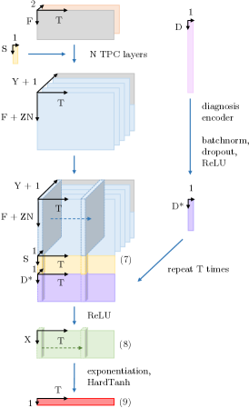
Figure 2: Overview of the framework used for the TPC model and the baselines. F, T, Y^∗, Z^∗, Z_t and $f$ are defined in the caption to Figure 1. The original time series (grey) along with the decay indicators (orange) (explained under ‘Time Series’ in Section A.4) are processed by $n$ TPC layers. If a baseline model were used instead of TPC, the time series output dimensions would be M x T, where M is the LSTM hidden size or $d_{model}$ in the Transformer (this is in place of the light blue and grey output in the TPC model). The diagnoses, $d$, are embedded by a diagnosis encoder – a single fully connected layer of size D. The time series (blue and grey), diagnosis embedding (purple) and flat features (yellow) are concatenated along the feature axis, and a two-layer pointwise convolution is applied to obtain the final predictions (red).

Figure 2 shows the full architecture. With each successive TPC layer, we increase the temporal dilation by 1. After processing the time series, we combine them with flat (non time-varying) features and a diagnosis embedding (Figure 2 shows the complete architecture). The combined features pass through a small two-layer pointwise convolution to obtain the LoS predictions. We apply an exponential function before the predictions are returned. This is intended to help to circumvent a common issue seen in previous models (e.g. Harutyunyan et al. (2019), as they struggle to produce predictions over the full range of length of stays). It effectively allows the upstream network to model $\log(\text{LoS})$ instead of LoS. This distribution is much closer to a Gaussian distribution than the remaining LoS distribution. We use batch normalisation (Ioffe and Szegedy, 2015) and dropout (Srivastava et al., 2014) to regularise the model. The hyperparameter search methodology is described in Section A.6. Finally, we apply a HardTanh function (Gülçehre et al., 2016) to the output to clip any predictions that are smaller than 30 minutes or larger than 100 days, which protects against inflated loss values:

$$\text{HardTanh}(x)=\begin{cases}100,&\text{if }x~{}\text{\textgreater}~{}100,\\ \frac{1}{48},&\text{if }x~{}\text{\textless}~{}\frac{1}{48},\\ x,&\text{otherwise.}\end{cases}$$

A.2 Remaining Length of Stay Task

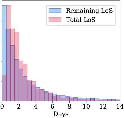
Figure 3: Total and remaining length of stay distributions. The mean and median values are (2.99, 1.82) and (3.47, 1.67) days respectively.

We assign a remaining LoS target to each hour of the stay, beginning 5 hours after admission to the ICU and ending when the patient dies or is discharged. The remaining LoS is calculated by subtracting the time elapsed in the ICU from the total LoS. We only train on data within the first 14 days of any patient’s stay to protect against batches becoming overly long and slowing down training. This cut-off applies to 2.4% of patient stays, but it does not affect their maximum remaining length of stay values because these appear within the first 14 days. The remaining LoS distribution is shown in Figure 3.

A.3 Feature Selection

We selected time series variables from the following tables: lab, nursecharting, respiratorycharting, vitalperiodic and vitalaperiodic. We used a semi-automatic process for feature selection. To be included, the variable had to be present in at least 12.5% of patient stays, or 25% of stays for lab variables. The lab table contains a much larger number of variables than the other tables, and they tend to be sparsely sampled (once per day or less). We extracted diagnoses from the pasthistory, admissiondx and diagnoses tables, and 17 flat (non time-varying) features from the patient, apachepatientresult and hospital tables (see Table 2).

Table 2: Flat features used in the model. Age >89, Null Height and Null Weight were added as indicator variables to indicate when the age was more than 89 but has been capped, and when the height or weight were missing and have been imputed with the mean value.

Feature	Type	Source Table
Gender	Binary	patient
Age	Discrete	patient
Hour of Admission	Discrete	patient
Height	Continuous	patient
Weight	Continuous	patient
Ethnicity	Categorical	patient
Unit Type	Categorical	patient
Unit Admit Source	Categorical	patient
Unit Visit Number	Categorical	patient
Unit Stay Type	Categorical	patient
Num Beds Category	Categorical	hospital
Region	Categorical	hospital
Teaching Status	Binary	hospital
Physician Speciality	Categorical	apachepatientresult
Age >89	Binary
Null Height	Binary
Null Weight	Binary

A.4 Feature Pre-processing

Flat Features

Discrete and continuous variables were scaled to the interval [-1, 1], using the 5th and 95th percentiles as the boundaries, and absolute cut offs were placed at [-4, 4]. This was to protect against large or erroneous inputs, while avoiding assumptions about the variable distributions. Binary variables were coded as 1 and 0. Categorical variables were converted to one-hot encodings.

Time Series

For each admission, 87 time-varying features (Table 3) were extracted from each hour of the ICU visit, and up to 24 hours before the ICU visit. The variables were processed in the same manner as the flat features. In general, the sampling is very irregular, so the data was re-sampled according to one hour intervals. Where there is missingness, we forward-fill to bridge the gaps in the data. After forward-filling is complete, any data recorded before the ICU admission is removed. To inform the model about where the data is stale, we add a ‘decay indicator’ to each feature to track how long it has been since a genuine observation was recorded. The decay is calculated as $0.75^{t}$, where $t$ is the time since the last recording. If it is up to date, decay is 1, and if it cannot be forward-filled, decay is 0. This is similar in spirit to the masking used by Che et al. (2018). A real example is shown in Figure 4.

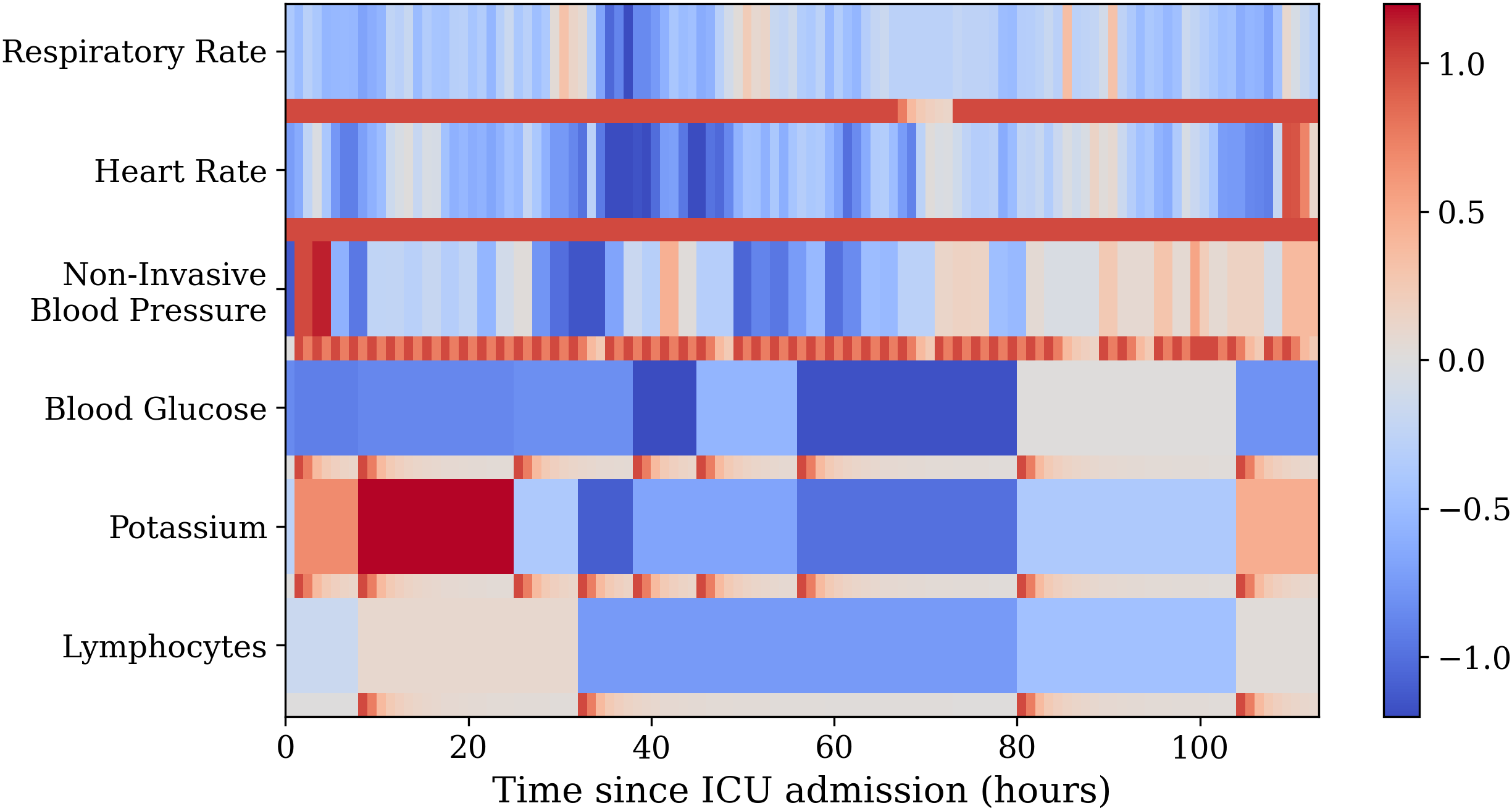
Figure 4: A selection of variables from one patient (after pre-processing). The colour scale indicates the value of the feature. Each feature is accompanied by its decay indicator (narrow bar underneath). Blood Glucose, Potassium and Lymphocytes are all laboratory tests. These are performed approximately once per day but we can see that the frequency is irregular. Non-invasive blood pressure is a variable that is recorded by the nurse. The sampling frequency is around 2 hours and is quite consistent. Respiratory Rate and Heart Rate are vital signs that are automatically logged at regular intervals.

Table 3: Time Series features. ‘Time in the ICU’ and ‘Time of day’ were not part of the tables in eICU but were added later as helpful indicators to the model.

Source Table
lab			respiratorycharting
-basos	MPV	glucose	Exhaled MV
-eos	O2 Sat (%)	lactate	Exhaled TV (patient)
-lymphs	PT	magnesium	LPM O2
-monos	PT - INR	pH	Mean Airway Pressure
-polys	PTT	paCO2	Peak Insp. Pressure
ALT (SGPT)	RBC	paO2	PEEP
AST (SGOT)	RDW	phosphate	Plateau Pressure
BUN	WBC x 1000	platelets x 1000	Pressure Support
Base Excess	albumin	potassium	RR (patient)
FiO2	alkaline phos.	sodium	SaO2
HCO3	anion gap	total bilirubin	TV/kg IBW
Hct	bedside glucose	total protein	Tidal Volume (set)
Hgb	bicarbonate	troponin - I	Total RR
MCH	calcium	urinary specific gravity	Vent Rate
MCHC	chloride
MCV	creatinine
nursecharting	vitalperiodic	vitalaperiodic	N/A
Bedside Glucose	cvp	noninvasivediastolic	Time in the ICU
Delirium Scale/Score	heartrate	noninvasivemean	Time of day
Glasgow coma score	respiration	noninvasivesystolic
Heart Rate	sao2
Invasive BP	st1
Non-Invasive BP	st2
O2 Admin Device	st3
O2 L/%	systemicdiastolic
O2 Saturation	systemicmean
Pain Score/Goal	systemicsystolic
Respiratory Rate	temperature
Sedation Score/Goal
Temperature

Diagnoses

Like many EHRs, diagnosis coding in eICU is hierarchical. At the lowest level they can be quite specific e.g. “neurologic $|$ disorders of vasculature $|$ stroke $|$ hemorrhagic stroke $|$ subarachnoid hemorrhage $|$ with vasospasm”. To maintain the hierarchical structure within a flat vector, we assigned separate features to each hierarchical level and use binary encoding. This produces a vector of size 4,436 with an average sparsity of 99.5% (only 0.5% of the data is positive). We apply a 1% prevalence cut-off on all these features to reduce the size of the vector to 293 and the average sparsity to 93.3%. If a disease does not make the cut-off for inclusion, it is still included via any parent classes that do make the cut-off (in the above example we record everything up to “subarachnoid hemorrhage”). We only included diagnoses that were recorded before the 5th hour in the ICU, to avoid leakage from the future.

Many diagnostic and interventional coding systems are hierarchical in nature: ICD-10 classification (World Health Organisation, 2011), Clinical Classifications Software (Elixhauser et al., 2015), SNOMED CT (De Silva et al., 2011) and OPCS Classification of Interventions and Procedures (NHS Digital, 2019), so this technique is generalisable to other coding systems present in EHRs.

A.5 Baselines

A certain level of performance is achievable ‘for free’ just by predicting values that are close to the mean or median LoS (3.50 and 1.70 days respectively). We include these static models as elemental baselines. Our ‘stronger’ baselines are a two-layer Long-Short Term Memory network (LSTM) (Hochreiter and Schmidhuber, 1997), a two-layer channel-wise LSTM, and a Transformer encoder network (Vaswani et al., 2017) (see Section A.6 for their hyperparameters).

Our standard LSTM baseline is very similar to the one used in a recent eICU benchmark paper including LoS prediction (Sheikhalishahi et al., 2019). The channel-wise LSTM (CW LSTM) consists of a set of independent LSTMs that process each feature separately. Like our TPC model, the CW LSTM has independent parameters dedicated to each time series feature. In theory, it should be able to cope better with irregular sampling and varying frequencies in the data, but it may be hindered by the inability to compute cross-feature interactions along the way. Harutyunyan et al. (2019) found that they performed better than the standard LSTM.

The Transformer was shown to perform marginally better than the standard LSTM when predicting LoS (Song et al., 2018). It is a multi-head self-attention model, originally designed for sequence-to-sequence tasks in natural language processing. It consists of both an encoder and decoder, however we only use the former because the LoS task is regression. Our implementation is the same as the original encoder in Vaswani et al. (2017), except that we add temporal masking to impose causality, and we omit the positional encodings because they were not helpful for the LoS task (see Table 6). Hypothetically, the Transformer shares an advantage with TPC in that it is not constrained to progress one timestep at a time. However, it is not able to scale its receptive fields in the same way as TPC and it does not have independent parameters per feature.

In all network baselines, the data (including decay indicators) and the non-time series components of the models were the same as in TPC (Figure 2).

A.6 Hyperparameter Search

Our model and its baselines have hyperparameters that can broadly be split into three categories: time series specific, non-time series specific and global parameters (shown in more detail in Tables 4, 5 and 6). The hyperparameter search ranges have been included in Table 7. First, we ran 25 randomly sampled hyperparameter trials on the TPC model to decide the non-time series specific parameters (diagnosis embedding size, final fully connected layer size, batch normalisation strategy and dropout rate) keeping all other parameters fixed. These parameters then remained fixed for all the models which share their non-time series specific architecture. We ran 50 hyperparameter trials to optimise the remaining parameters for the TPC, standard LSTM, and Transformer models. To train the channel-wise LSTM and the temporal model with weight sharing, we ran a further 10 trials to re-optimise the hidden size (8 per feature) and number of temporal channels (32 channels shared across all features) respectively. For all other ablation studies and variations of each model, we kept the same hyperparameters where applicable (see Table 1 for a full list of all the models). The number of epochs was determined by selecting the best validation performance from a model trained over 50 epochs. This was different for each model: 8 for LSTM, 30 for CW LSTM, and 15 for the Transformer and TPC models. We noted that the best LSTM hyperparameters were similar to that found in Sheikhalishahi et al. (2019). We used trixi to structure our experiments and easily compare different hyperparameter choices (Zimmerer et al., 2017). All deep learning methods were implemented in PyTorch (Paszke et al., 2019) and were optimised using Adam (Kingma and Ba, 2014).

Table 4: The TPC model has 11 hyperparameters (Main Dropout and Batch Normalisation have been repeated in the table because they apply to multiple parts of the model). We allowed the model to optimise a custom dropout rate for the temporal convolutions because they have fewer parameters and might need less regularisation than the rest of the model. The best hyperparameter values are shown in brackets. Hyperparameters marked with * were fixed across all of the models.

TPC Specific
Temporal Specific	Pointwise Specific
Temp. Channels (12)	Point. Channels (13)
Temp. Dropout (0.05)	Main Dropout* (0.45)
Kernel Size (4)
Batch Normalisation* (True)
No. TPC Layers (9)
Non-TPC Specific	Global Parameters
Diag. Embedding Size* (64)	Batch Size (32)
Main Dropout* (0.45)	Learning Rate (0.00226)
Final FC Layer Size* (17)
Batch Normalisation* (True)

Table 5: The LSTM model has 9 hyperparameters. We allowed the model to optimise a custom dropout rate for the LSTM layers. Note that batch normalisation is not applicable to the LSTM layers. The best hyperparameter values are shown in brackets. Hyperparameters marked with * were fixed across all of the models.

LSTM Specific	Non-LSTM Specific	Global Parameters
Hidden State (128)	Diag. Embedding Size* (64)	Batch Size (512)
LSTM Dropout (0.2)	Main Dropout* (0.45)	Learning Rate (0.00129)
No. LSTM Layers (2)	Final FC Layer Size* (17)
	Batch Normalisation* (True)

Table 6: The Transformer model has 12 hyperparameters. We allowed the model to optimise a custom dropout rate for the Transformer layers. The positional encoding hyperparameter is binary; it determines whether or not we used the original positional encodings proposed by Vaswani et al. (2017). They were not found to be helpful (perhaps because we already have a feature to indicate the position in the time series (Section A.4)). Note that batch normalisation is not applicable to the Transformer layers (the default implementation uses layer normalisation). The best hyperparameter values are shown in brackets. Hyperparameters marked with * were fixed across all of the models.

Transformer Specific	Non-Transformer Specific	Global Parameters
No. Attention Heads (2)	Diag. Embedding Size* (64)	Batch Size (32)
Feedforward Size (256)	Main Dropout* (0.45)	Learning Rate (0.00017)
$d_{model}$ (16)	Final FC Layer Size* (17)
Positional Encoding (False)	Batch Normalisation* (True)
Transformer Dropout (0)
No. Transformer Layers (6)

Table 7: Hyperparameter Search Ranges. We took a random sample from each range and converted to an integer if necessary. For the kernel sizes (not shown in the table) the range was dependent on the number of TPC layers selected (because large kernel sizes combined with a large number of layers can have an inappropriately wide range as the dilation factor increases per layer). In general the range of kernel sizes was around 2-5 (but it could be up to 10 for small numbers of TPC Layers).

Hyperparameter	Lower	Upper	Scale
Batch Size	4	512	$\log_{2}$
Dropout Rate (all)	0	0.5	Linear
Learning Rate	0.0001	0.01	$\log_{10}$
Batch Normalisation	True	False
Positional Encoding	True	False
Diagnosis Embedding Size	16	64	$\log_{2}$
Final FC Layer Size	16	64	$\log_{2}$
Channel-Wise LSTM Hidden State Size	4	16	$\log_{2}$
Point. Channels	4	16	$\log_{2}$
Temp. Channels	4	16	$\log_{2}$
Temp. Channels (weight sharing)	16	64	$\log_{2}$
LSTM Hidden State Size	16	256	$\log_{2}$
$d_{model}$	16	256	$\log_{2}$
Feedforward Size	16	256	$\log_{2}$
No. Attention Heads	2	16	$\log_{2}$
No. TPC Layers	1	12	Linear
No. LSTM Layers	1	4	Linear
No. Transformer Layers	1	10	Linear

Appendix B Evaluation Metrics

The metrics we use are: mean absolute deviation (MAD), mean absolute percentage error (MAPE), mean squared error (MSE), mean squared loss error (MSLE), coefficient of determination ($R^{2}$) and Cohen Kappa Score. We use 6 different metrics because there is a risk that bad models can ‘cheat’ particular metrics just by virtue of being close to the mean or median value, or by not predicting long length of stays. This is not what we want in a bed management model, because long length of stays are disproportionately important due to their lasting effect on occupancy.

We have modified the MAPE metric slightly so that very small true LoS values do not produce unbounded MAPE values. We place a 4 hour lower bound on the divisor i.e.

$$\text{Absolute Percentage Error}=\mathinner{\!\left\lvert\frac{y_{true}-y_{pred}}{\max{(y_{true},\frac{4}{24})}}\right\rvert}*100$$

MAD and MAPE are improved by centering predictions on the median. Likewise, MSE and $R^{2}$ are bettered by centering predictions around the mean. They are more affected by the skew. MSLE is a good metric for this task, indeed, it is the loss function in most experiments, but is less readily-interpretable than some of the other measures. Cohen’s linear weighted Kappa Score (Cohen, 1960) is intended for ordered classification tasks rather than regression, but it can effectively mitigate for skew if the bins are chosen well. It has previously provided useful insights in Harutyunyan et al. (2019), so we use the same LoS bins: 0-1, 1-2, 2-3, 3-4, 4-5, 5-6, 6-7, 7-8, 8-14, and 14+ days. As a classification measure, it will treat everything falling within the same classification bin as equal, so it is fundamentally a coarser measure than the other metrics.

To illustrate the importance of using multiple metrics, consider that the mean and median models are in some sense equally poor (neither has learned anything meaningful for our purposes). Nevertheless, the median model is able to better exploit the MAD, MAPE and MSLE metrics, and the mean model fares better with MSE, but the Kappa score betrays them both. A good model will perform well across all of the metrics.

Appendix C Additional Investigations

C.1 Loss Function

Table 8: The effect of training with the mean squared logarithmic error (MSLE) loss function when compared to mean squared error (MSE). The metrics are defined in Section B. The colour scheme and confidence interval calculation is described in the legend to Table 1.

Model	MAD	MAPE	MSE	MSLE	$R^{2}$	Kappa
LSTM (MSLE)	2.39$\pm$0.00	118.2$\pm$1.1	26.9$\pm$0.1	1.47$\pm$0.01	0.09$\pm$0.00	0.28$\pm$0.00
LSTM (MSE)	2.57$\pm$0.03	235.2$\pm$6.2	24.5$\pm$0.2	1.97$\pm$0.02	0.17$\pm$0.01	0.28$\pm$0.01
CW LSTM (MSLE)	2.37$\pm$0.00	114.5$\pm$0.4	26.6$\pm$0.1	1.43$\pm$0.00	0.10$\pm$0.00	0.30$\pm$0.00
CW LSTM (MSE)	2.56$\pm$0.01	218.5$\pm$4.0	24.2$\pm$0.1	1.84$\pm$0.02	0.18$\pm$0.00	0.34$\pm$0.01
Transformer (MSLE)	2.36$\pm$0.00	114.1$\pm$0.6	26.7$\pm$0.1	1.43$\pm$0.00	0.09$\pm$0.00	0.30$\pm$0.00
Transformer (MSE)	2.51$\pm$0.01	212.7$\pm$5.2	24.7$\pm$0.2	1.87$\pm$0.03	0.16$\pm$0.01	0.28$\pm$0.01
TPC (MSLE)	1.78$\pm$0.02	63.5$\pm$4.3	21.7$\pm$0.5	0.70$\pm$0.03	0.27$\pm$0.02	0.58$\pm$0.01
TPC (MSE)	2.21$\pm$0.02	154.3$\pm$10.1	21.6$\pm$0.2	1.80$\pm$0.10	0.27$\pm$0.01	0.47$\pm$0.01

C.2 Skip Connections

We propagate skip connections (He et al., 2015) to allow each layer to see the original data and the pointwise outputs from previous layers. This helps the network to cope with sparsely sampled data. For example, suppose a particular blood test is taken once per day. In order to not to lose temporal resolution, we forward-fill these data (A.3) and convolve with increasingly dilated temporal filters until we find the appropriate width to capture a useful trend. However, if the smaller filters in previous layers (which did not see any useful trend) have polluted the original data by re-weighting, learning will be harder. Skip connections provide a consistent anchor to the input. They are concatenated (like in DenseNet (Huang et al., 2017), and are arranged in the shared-source connection formation (Wang et al., 2018)). The skip connections expand both the feature dimension to accommodate the pointwise outputs, and the channel dimension to fit the original data. This is best visualised in Figure 1. We can see from Table 9 that removing the skip connections reduces performance by 5-25%.

Table 9: The effect of skip connections. The metrics are defined in Section B. The colour scheme and confidence interval calculation is described in the legend to Table 1.

Model	MAD	MAPE	MSE	MSLE	$R^{2}$	Kappa
TPC	1.78$\pm$0.02 ∗∗	63.5$\pm$3.8 ∗∗	21.8$\pm$0.5 ∗∗	0.71$\pm$0.03 ∗∗	0.26$\pm$0.02 ∗∗	0.58$\pm$0.01 ∗∗
TPC (no skip)	1.93$\pm$0.01	73.9$\pm$1.9	23.0$\pm$0.2	0.89$\pm$0.01	0.22$\pm$0.01	0.51$\pm$0.01

References

- Blom et al. (2015) Mathias C. Blom, Karin Erwander, Lars M. Gustafsson, Mona Landin-Olsson, Fredrik Jonsson, and Kjell Ivarsson. The Probability of Readmission within 30 days of Hospital Discharge is Positively Associated with Inpatient Bed Occupancy at Discharge – A Retrospective Cohort Study. In BMC Emergency Medicine, 2015.
- Che et al. (2018) Zhengping Che, Sanjay Purushotham, Kyunghyun Cho, David Sontag, and Yan Liu. Recurrent Neural Networks for Multivariate Time Series with Missing Values. Scientific Reports, 8(1):6085, 2018.
- Choi et al. (2015) Edward Choi, Mohammad Taha Bahadori, Andy Schuetz, Walter F. Stewart, and Jimeng Sun. Doctor AI: Predicting Clinical Events via Recurrent Neural Networks. JMLR workshop and conference proceedings, 56:301–318, 2015.
- Chollet (2016) François Chollet. Xception: Deep Learning with Depthwise Separable Convolutions. CoRR, abs/1610.02357, 2016.
- Cohen (1960) Jacob Cohen. A Coefficient of Agreement for Nominal Scales. Educational and Psychological Measurement, 20(1):37–46, 1960.
- De Silva et al. (2011) Thuppahi Sisira De Silva, Don MacDonald, Grace Paterson, Khokan C. Sikdar, and Bonnie Cochrane. Systematized Nomenclature of Medicine Clinical Terms (SNOMED CT) to Represent Computed Tomography Procedures. Comput. Methods Prog. Biomed., 101(3):324–329, 2011.
- Elixhauser et al. (2015) A Elixhauser, C Steiner, and L Palmer. Clinical Classifications Software, 2015.
- Gülçehre et al. (2016) Çaglar Gülçehre, Marcin Moczulski, Misha Denil, and Yoshua Bengio. Noisy Activation Functions. CoRR, abs/1603.00391, 2016.
- Harutyunyan et al. (2019) Hrayr Harutyunyan, Hrant Khachatrian, David C. Kale, Greg Ver Steeg, and Aram Galstyan. Multitask Learning and Benchmarking with Clinical Time Series Data. Scientific Data, 6(96), 2019.
- Hassan et al. (2010) Mahmud Hassan, Howard Tuckman, Robert Patrick, David Kountz, and Jennifer Kohn. Hospital Length of Stay and Probability of Acquiring Infection. International Journal of Pharmaceutical and Healthcare Marketing, 4:324–338, 2010.
- He et al. (2015) Kaiming He, Xiangyu Zhang, Shaoqing Ren, and Jian Sun. Deep Residual Learning for Image Recognition. CoRR, abs/1512.03385, 2015.
- Hochreiter and Schmidhuber (1997) Sepp Hochreiter and Jürgen Schmidhuber. Long Short-Term Memory. Neural computation, 9(8):1735–1780, 1997.
- Huang et al. (2017) Gao Huang, Zhuang Liu, Laurens van der Maaten, and Kilian Q Weinberger. Densely connected convolutional networks. In Proceedings of the IEEE Conference on Computer Vision and Pattern Recognition, 2017.
- Ioffe and Szegedy (2015) Sergey Ioffe and Christian Szegedy. Batch normalization: Accelerating deep network training by reducing internal covariate shift. In Proceedings of the 32nd International Conference on International Conference on Machine Learning - Volume 37, ICML’15, pages 448–456. JMLR, 2015.
- Kalchbrenner et al. (2016) Nal Kalchbrenner, Lasse Espeholt, Karen Simonyan, Aäron van den Oord, Alex Graves, and Koray Kavukcuoglu. Neural Machine Translation in Linear Time. CoRR, abs/1610.10099, 2016.
- Kingma and Ba (2014) Diederik P. Kingma and Jimmy Ba. Adam: A method for stochastic optimization. CoRR, abs/1412.6980, 2014.
- Laupland et al. (2006) Kevin B. Laupland, Andrew W. Kirkpatrick, John B. Kortbeek, and Danny J. Zuege. Long-term Mortality Outcome Associated With Prolonged Admission to the ICU. Chest, 129(4):954 – 959, 2006.
- Lin et al. (2013) Min Lin, Qiang Chen, and Shuicheng Yan. Network In Network, 2013.
- Lipton et al. (2015) Zachary Chase Lipton, David C. Kale, Charles Elkan, and Randall C. Wetzel. Learning to Diagnose with LSTM Recurrent Neural Networks. CoRR, abs/1511.03677, 2015.
- Mak et al. (2012) Gregory Mak, William D. Grant, James C McKenzie, and John B. Mccabe. Physicians’ Ability to Predict Hospital Length of Stay for Patients Admitted to the Hospital from the Emergency Department. In Emergency medicine international, 2012.
- Nassar and Caruso (2016) Antonio Paulo Nassar and Pedro Caruso. ICU Physicians are Unable to Accurately Predict Length of Stay at Admission: A Prospective Study. Journal of the International Society for Quality in Health Care, 28 1:99–103, 2016.
- NHS Digital (2019) NHS Digital. DCB0084: OPCS-4.9 Requirements Specification, 2019.
- Paszke et al. (2019) Adam Paszke, Sam Gross, Francisco Massa, et al. PyTorch: An Imperative Style, High-Performance Deep Learning Library. In Advances in Neural Information Processing Systems 32, pages 8024–8035. Curran Associates, Inc., 2019.
- Pollard et al. (2018) Tom J Pollard, Alistair E W Johnson, Jesse D Raffa, Leo A Celi, Roger G Mark, and Omar Badawi. The eICU Collaborative Research Database, A Freely Available Multi-Center Database for Critical Care Research. Scientific Data, 5(1):180178, 2018.
- Rajkomar et al. (2018) Alvin Rajkomar, Eyal Oren, Kai Chen, et al. Scalable and Accurate Deep Learning with Electronic Health Records. In npj Digital Medicine, 2018.
- Rapoport et al. (2003) John Rapoport, Daniel Teres, Yonggang Zhao, and Stanley Lemeshow. Length of Stay Data as a Guide to Hospital Economic Performance for ICU Patients. Medical Care, 41:386–397, 2003.
- Sheikhalishahi et al. (2019) Seyedmostafa Sheikhalishahi, Vevake Balaraman, and Venet Osmani. Benchmarking Machine Learning Models on eICU Critical Care Dataset, 2019.
- Shickel et al. (2019) Benjamin Shickel, Tyler J. Loftus, Lasith Adhikari, Tezcan Ozrazgat-Baslanti, Azra Bihorac, and Parisa Rashidi. DeepSOFA: A Continuous Acuity Score for Critically Ill Patients using Clinically Interpretable Deep Learning. In Scientific Reports, 2019.
- Song et al. (2018) Huan Song, Deepta Rajan, Jayaraman J. Thiagarajan, and Andreas Spanias. Attend and Diagnose: Clinical Time Series Analysis using Attention Models. In 32nd AAAI Conference on Artificial Intelligence, AAAI 2018, pages 4091–4098. AAAI press, 2018.
- Srivastava et al. (2014) Nitish Srivastava, Geoffrey Hinton, Alex Krizhevsky, Ilya Sutskever, and Ruslan Salakhutdinov. Dropout: A Simple Way to Prevent Neural Networks from Overfitting. Journal of Machine Learning Research, 15:1929–1958, 2014.
- Szegedy et al. (2014) Christian Szegedy, Wei Liu, Yangqing Jia, Pierre Sermanet, Scott E. Reed, Dragomir Anguelov, Dumitru Erhan, Vincent Vanhoucke, and Andrew Rabinovich. Going Deeper with Convolutions. CoRR, abs/1409.4842, 2014.
- van den Oord et al. (2016) Aäron van den Oord, Sander Dieleman, Heiga Zen, Karen Simonyan, Oriol Vinyals, Alex Graves, Nal Kalchbrenner, Andrew W. Senior, and Koray Kavukcuoglu. WaveNet: A Generative Model for Raw Audio. CoRR, abs/1609.03499, 2016.
- Vaswani et al. (2017) Ashish Vaswani, Noam Shazeer, Niki Parmar, Jakob Uszkoreit, Llion Jones, Aidan N. Gomez, undefinedukasz Kaiser, and Illia Polosukhin. Attention is all you need. In Proceedings of the 31st International Conference on Neural Information Processing Systems, NIPS’17, page 6000–6010. Curran Associates Inc., 2017.
- Wang et al. (2018) Zhongyuan Wang, Peng Yi, Kui Jiang, Junjun Jiang, Zhen Han, Tao Lu, and Jiayi Ma. Multi-memory convolutional neural network for video super-resolution. IEEE Transactions on Image Processing, PP:1–1, 12 2018. 10.1109/TIP.2018.2887017.
- World Health Organisation (2011) World Health Organisation. ICD-10: International Statistical Classification of Diseases and Related Health Problems, volume 10th Revision. World Health Organision, 2011.
- Zimmerer et al. (2017) David Zimmerer, Jens Petersen, Gregor Köhler, Jakob Wasserthal, Tim Adler, Sebastian Wirkert, and Tobias Ross. trixi - Training and Retrospective Insight eXperiment Infrastructure. https://github.com/MIC-DKFZ/trixi, 2017.