Bulk-and-edge to corner correspondence

Abstract

We show that two-dimensional band insulators, with vanishing bulk polarization, obey bulk-and-edge to corner charge correspondence, stating that the knowledge of the bulk and the two corresponding ribbon band structures uniquely determines a fractional part of the corner charge irrespective of the corner termination. Moreover, physical observables related to macroscopic charge density of a terminated crystal can be obtained by representing the crystal as collection of polarized edge regions with polarizations $\vec{P}^{\text{edge}}_{\alpha}$, where the integer $\alpha$ enumerates the edges. We introduce a particular manner of cutting a crystal, dubbed “Wannier cut”, which allows us to compute $\vec{P}^{\text{edge}}_{\alpha}$. We find that $\vec{P}^{\text{edge}}_{\alpha}$ consists of two pieces: the bulk piece expressed via quadrupole tensor of the bulk Wannier functions’ charge density and the edge piece corresponding to the Wannier edge polarization—the polarization of the edge subsystem obtained by Wannier cut. For a crystal with $n$ edges, out of $2n$ independent components of $\vec{P}^{\text{edge}}_{\alpha}$, only $2n-1$ are independent of the choice of Wannier cut and correspond to physical observables: corner charges and edge dipoles.

I Introduction

While the bulk description of solid-state materials is generally available, the description close to the material’s boundaries (termination) is often not accessible. For this reason, a particularly important role for material science is played by bulk quantities—they depend only on the material’s bulk although they predict a certain quantity that can be measured once a boundary is introduced. In other words, the sole existence of the bulk quantities requires some form of bulk-boundary correspondence. To name a few examples, the bulk electrical polarization of an insulator predicts a fractional part of the end charge Resta and Vanderbilt (2007); King-Smith and Vanderbilt (1993); Vanderbilt and King-Smith (1993); Resta (1994); Resta and Sorella (1999), the bulk orbital magnetization Thonhauser et al. (2005); Shi et al. (2007) predicts persistent current circulating along the boundary, bulk geometric orbital magnetization Trifunovic et al. (2019) predicts a fractional part of the time-averaged edge current circulating along the boundary of a periodically, adiabatically driven insulator, and the bulk magnetoelectric polarizability of a three-dimensional insulator predicts a fractional part of the surface charge density resulting from the application of an external magnetic field. Qi et al. (2008); Essin et al. (2009)

In recent years, Kitaev (2009); Schnyder et al. (2009) the term bulk-boundary correspondence is almost exclusively used in the context of topological phenomena. In that more strict sense, the bulk-boundary correspondence assumes that the bulk quantity is topological invariant; hence, the boundary quantity is quantized. Notable examples include quantum (spin) Hall effect where Chern number (Kane-Mele invariant Kane and Mele (2005a)) predicts quantized (spin) Hall conductance, Thouless et al. (1982); Kane and Mele (2005b); Bernevig et al. (2006), and $\mathbb{Z}_{2}$ invariant predicting quantized zero-energy conductance of the Kitaev chain. Kitaev (2001); Alicea et al. (2011); Lutchyn et al. (2010); Mourik et al. (2012) In this work, such correspondence is referred to as topological bulk-boundary correspondence. Schnyder et al. (2009); Shiozaki et al. (2018); Trifunovic and Brouwer (2019); Roberts et al. (2020); Trifunovic and Brouwer (2020) In certain cases bulk-boundary correspondence can be enriched by the attribute “topological” in the presence of certain symmetries: The bulk polarization and a fractional part of the end charge become quantized in the presence of inversion symmetry, the bulk geometric orbital magnetization and a fractional part of the time-averaged edge current are quantized in the presence of inversion or fourfold rotation symmetry, Trifunovic et al. (2019) and similarly, the magnetoelectric polarizability and the associated boundary quantity are quantized in the presence of time-reversal or inversion symmetry. Qi et al. (2008) On the other hand, no symmetry quantizes the bulk orbital magnetization. It may be of interest to ask a reverse question: In which cases a topological bulk-boundary correspondence can be extended to its unquantized version? This work deals with one example where such an extension is not possible—the bulk quadrupole moment and the corner charge. Namely, in the presence of fourfold rotation symmetry, the bulk quadrupole moment is topological invariant and predicts the quantized corner charge, Benalcazar et al. (2017) whereas in the absence of this symmetry constraint it is not possible to predict the corner charge without specifying the edge terminations. Ono et al. (2019) In this work, we show that instead of bulk to boundary correspondence, a bulk-and-edge to corner correspondence can be formulated.

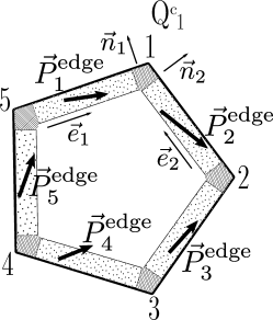
Figure 1: Illustration of a crystal with boundary. To obtain a fractional part of each of the five corners (hatched regions), the bulk and the five edge terminations (dotted regions) need to be specified, while the termination around the corners need not be specified. The edges run along the lattice vectors $\vec{e}_{\alpha}$, with the unit normal vectors $\vec{n}_{\alpha}$ pointing outward, $\alpha=1,\dots,5$. The corner charge, where the edges along $\vec{e}_{\alpha}$ and $\vec{e}_{\alpha+1}$ meet, is denoted by $Q_{\alpha}^{\text{c}}$. The macroscopic charge density of a crystal can be seen to be generated by a collection of polarized edge regions (dotted) with polarizations $\vec{P}^{\text{edge}}_{\alpha}$. The charge neutrality and vanishing bulk polarization are assumed; hence, $\sum_{\alpha}Q^{\text{c}}_{\alpha}=0$, whereas $\sum_{\alpha}\vec{P}^{\text{edge}}_{\alpha}$ need not vanish.

In 2015, Zhou, Rabe, and Vanderbilt Zhou et al. (2015) proposed that for band insulators, a fractional part of the corner charge $Q^{\text{c}}$ can be computed from the knowledge of the bulk and the two corresponding ribbon band structures via the following relation:

$$Q^{\text{c}} =P^{\text{edge}}_{x}+P^{\text{edge}}_{y}\mod e,$$ (1)

where $P^{\text{edge}}_{x}$ ($P^{\text{edge}}_{y}$) is the $x$ component ($y$ component) of the edge polarization for the edge along the $x$ ($y$) direction. These authors defined the edge polarization in terms of so-called maximally localized hybrid Wannier functions, Marzari et al. (2012) and verified the relation (1) using two tight-binding models. Zhou et al. (2015) One year later, in their pioneering work, Benalcazar, Bernevig, and Hughes proposed the model Benalcazar et al. (2017) that in the presence of fourfold rotation symmetry Benalcazar et al. (2019) exhibits quantized corner charge that is given by topological invariant dubbed “bulk quadrupole moment” $q_{xy}$,

$$q_{xy} =Q^{\text{c}}-P^{\text{edge}}_{x}-P^{\text{edge}}_{y}\mod e,$$ (2)

with $P^{\text{edge}}_{x,y}$ defined in the same manner as in Eq. (1). The nonvanishing value of “$Q^{\text{c}}-P^{\text{edge}}_{x}-P^{\text{edge}}_{y}$” proves that previously proposed relation (1) cannot hold in general. Note that fourfold rotation symmetry forces the relation $P^{\text{edge}}_{x}=-P^{\text{edge}}_{y}\mod e$ to hold, and hence the $q_{xy}=Q^{\text{c}}\mod e$ which expresses topological bulk-boundary correspondence. Subsequent works Wheeler et al. (2019); Kang et al. (2019) by two independent groups proposed an expression that was meant to predict $q_{xy}$ in the absence of the symmetry constraints, using the bulk Hamiltonian as its sole input. These findings were supported by calculations on several tight-binding models. Wheeler et al. (2019); Kang et al. (2019) Shortly after, Ono, Watanabe, and the present author provided counterexamples showing that the proposed expression does not hold in general. In this work, we show that there exists no unique value for $q_{xy}$, since the edge polarizations in Eq. (2) are not uniquely defined quantities.

This work considers two-dimensional band insulators with a well-defined corner charge, which is the case when not only the bulk but also the boundary is gapped and the edge charge density vanishes. Figure 1 shows one example of a terminated crystal, with the index $\alpha$ enumerating the corners. Two edges, along lattice vectors $\vec{e}_{\alpha}$ and $\vec{e}_{\alpha+1}$ with the corresponding unit normal vectors $\vec{n}_{\alpha}$ and $\vec{n}_{\alpha+1}$, meet at the corner with the index $\alpha$. The main result of this work is finding that the physical observables related to macroscopic Jackson (1999) charge density $\rho^{\text{macro}}$ of such terminated crystal—corner charges and edge dipoles—can be obtained by representing the crystal as a collection of edge regions with polarizations $\vec{P}^{\text{edge}}_{\alpha}$; see Fig. 1. We find that the edge polarizations $\vec{P}^{\text{edge}}_{\alpha}$ consist of two pieces,

$$\vec{P}^{\text{edge}}_{\alpha}= L_{\alpha}\hat{q}\cdot\vec{n}_{\alpha}/2+\vec{\mathfrak{P}}^{\text{edge}}_{\alpha},$$ (3)

with $L_{\alpha}=|\vec{e}_{\alpha}|$ being the shortest repeated length along the $\alpha$ direction. The quadrupole tensor density $\hat{q}$ (bulk piece) is defined as the quadrupole tensor of the charge density of the bulk Wannier functions divided by the area of the unit cell. The Wannier edge polarization $\vec{\mathfrak{P}}^{\text{edge}}_{\alpha}$ is obtained from the corresponding ribbon band structure by performing a “Wannier cut“; see Sec. III.2 for the precise definition. For a crystal in with $n$ edges, there are $n$ edge polarizations with $2n$ independent components; out of those $2n-1$ are independent of the choice of Wannier cut (see Sec. III.3).

The result (3) turns the bulk-boundary correspondence for electrical polarization King-Smith and Vanderbilt (1993) into bulk-and-edge to corner correspondence

$$Q_{\alpha}^{\text{c}}= \frac{L_{\alpha+1}}{A_{\text{cell}}}\vec{P}^{\text{edge}}_{\alpha}\cdot\vec{n}_{\alpha+1}+\frac{L_{\alpha}}{A_{\text{cell}}}\vec{P}^{\text{edge}}_{\alpha+1}\cdot\vec{n}_{\alpha}\mod e,$$ (4)

where $A_{\text{cell}}=|\vec{e}_{\alpha}\times\vec{e}_{\alpha+1}|$ is the area of the unit cell defined by the corresponding corner.

The remaining of the article is organized as follows. In Sec. II, we review the modern theory of electrical polarizations and define corner charges and edge dipoles. Section III contains the main results of our work; therein we formulate and prove bulk-and-edge to corner charge correspondence and introduce the notion of Wannier cut and Wannier edge polarization. Three simple tight-binding models that illustrate the procedure described in Sec. III can be found in Sec. IV. We conclude in Sec. V.

II Preliminaries

We start by reviewing the distinction between microscopic and macroscopic charge density of a crystal. Section II.2 reviews the modern theory of electric polarization of band insulators and the corresponding bulk-boundary correspondence. Resta and Vanderbilt (2007); King-Smith and Vanderbilt (1993)

II.1 Macroscopic charge density. Corner charge and edge dipole.

The microscopic charge density $\rho({\vec{r}})$ of a crystal can change rapidly on a scale comparable or smaller than the size of its unit cell $a_{i}$. Hence, $\rho({\vec{r}})$ itself is not a physical observable but rather $\rho^{\text{macro}}({\vec{r}})$,  obtained by spatial averaging (convolution) from $\rho({\vec{r}})$, Jackson (1999); Vanderbilt (2018)

$$\rho^{\text{macro}}({\vec{r}})=\int d^{2}r^{\prime}\rho({\vec{r}}^{\prime})g({\vec{r}}-{\vec{r}}^{\prime}),$$ (5)

where $g({\vec{r}})$ is a normalized function, positive in the vicinity of ${\vec{r}}=0$. One possible choice is a Gaussian function, $g(\vec{r})=e^{-\frac{r^{2}}{2\xi^{2}}}/(\pi\xi^{2})$, where the spread $\xi>a_{i}$ should be chosen with some care. Namely, the crystal’s charge neutrality implies that $\rho^{\text{macro}}({\vec{r}})$ vanishes for $\vec{r}$ away from the crystal boundaries, which is satisfied with given accuracy only for a sufficiently large $\xi$.

As an example, consider a tight-binding model with eigenvectors $|\psi_{n}\rangle$. The microscopic charge distribution $\rho({\vec{r}})$ is obtained from the projector onto occupied states (i.e., ground-state density operator)

$${\cal P}({\vec{x}},{\vec{x}}^{\prime}) =\sum_{n\in\text{occ}}\psi_{n}^{*}({\vec{x}})\psi_{n}({\vec{x}}^{\prime}),$$ (6)

as

$$\rho({\vec{r}}) =-e\sum_{\vec{x}}{\cal P}({\vec{x}},{\vec{x}})\delta({\vec{r}}-{\vec{x}})+\rho^{\text{ion}}({\vec{r}}).$$ (7)

In the above equations, ${\vec{x}}$ runs over the sites of the tight-binding model, $\rho^{\text{ion}}({\vec{r}})$ is ionic charge distribution, and we modelled the charge distribution of electronic orbitals by $\delta$ function. The above microscopic charge density varies rapidly within the unit cell.

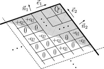
Figure 2: The macroscopic charge density $\rho^{\text{macro}}({\vec{r}})$ for ${\vec{r}}$ in the bulk, the two edges, and the corner regions. For clarity, the crystal is divided into cells (containing many unit cells) and the total charge in each cell is shown. The corner is defined by the two edges with the unit normal vectors $\vec{n}_{\alpha}$, $\alpha=1,2$. When either $D^{\text{edge}}_{1}$ or $D^{\text{edge}}_{2}$ are non-vanishing, integrating $\rho^{\text{macro}}$ over different corner regions ${\cal R}^{\text{c}}$, denoted by dashed lines and the hatched region, results in different corner charge.

In practice, even the macroscopic charge density $\rho^{\text{macro}}({\vec{r}})$ of a crystal in not directly measured but rather the features that can be extracted from it: the end or corner charges and the edge dipoles. Let us first consider a finite quasi-one-dimensional system with charge density $\rho^{\text{macro}}(r_{1})$, ${\vec{r}}=r_{1}{\vec{a}}_{1}$. Because of charge neutrality in the bulk, $\rho^{\text{macro}}(r_{1})$ is non-vanishing only for $r_{1}$ close to the ends of the crystal. We define the edge charge $Q^{\text{e}}$

$$Q^{\text{e}} =a_{1}\int dr_{1}\rho^{\text{macro}}(r_{1}),$$ (8)

where the integration region includes only one end. For a tight-binding model, $Q^{\text{e}}$ can be obtained from Eqs. (7) and (5) using Gaussian function with appropriately chosen $\xi$. Alternatively, as a more straightforward approach, one performs moving window average on $\rho$ which corresponds to the choice of $g(r_{1})$ in Eq. (5) to be unit-box function, having value $1/a_{1}$ within the unit cell at origin and zero otherwise. The result of this averaging procedure is (see Sec. 4.5 of Ref. Vanderbilt, 2018)

$$Q^{\text{e}} =a_{1}\int_{-\infty}^{\infty}dr_{1}f_{1}(r_{1})\rho(r_{1}),$$ (9)

where $f_{\alpha}(r)$ is the following ramp function,

$$f_{\alpha}(r) =\begin{cases}0&r<r_{0\alpha}\\ r-r_{0\alpha}&r_{0\alpha}\leq r\leq r_{0\alpha}+1\\ 1&\text{otherwise},\end{cases}$$ (10)

with $r_{0\alpha}$ far away from the ends.

Next, we consider finite two-dimensional (insulating) crystal that is charge neutral and with vanishing edge charge density. Under these assumptions, $\rho^{\text{macro}}({\vec{r}})$ has to vanish for ${\vec{r}}$ away from the boundaries, for ${\vec{r}}$ close to the middle of the edges there can be two spatially separated line charge densities of opposite signs, while for ${\vec{r}}$ close to the corners the macroscopic charge density is generally nonvanishing; see Fig. 2. Two features can be extracted from such $\rho^{\text{macro}}({\vec{r}})$: edge dipole and corner charge. The edge dipole $D^{\text{edge}}_{\alpha}$, for the edge along the lattice vector ${\vec{e}}_{\alpha}$ and with the unit normal vector $\vec{n}_{\alpha}$, is defined as

$$D^{\text{edge}}_{\alpha} =L_{\alpha}\int d({\vec{r}}\cdot\vec{n}_{\alpha}){\vec{r}}\cdot\vec{n}_{\alpha}\rho^{\text{macro}}({\vec{r}}),$$ (11)

where the integration line crosses around the middle of the edge and $L_{\alpha}=|{\vec{e}}_{\alpha}|$. The corner charge $Q_{\alpha}^{\text{c}}$ is defined as integral of macroscopic charge density over certain corner region ${\cal R}_{\alpha}^{\text{c}}$

$$Q_{\alpha}^{\text{c}} =\int_{{\cal R}_{\alpha}^{\text{c}}}d^{2}r\rho^{\text{macro}}({\vec{r}}).$$ (12)

Only for vanishing $D^{\text{edge}}_{\alpha}$ and $D^{\text{edge}}_{\alpha+1}$ is $Q_{\alpha}^{\text{c}}$ independent of the choice of ${\cal R}_{\alpha}^{\text{c}}$; see Fig. 2. The quantities (11) and (12) can be computed directly from microscopic charge density $\rho({\vec{r}})$ if a moving window average is performed with the “window” corresponding to the unit cell defined by the corresponding corner. The result for edge dipole is

$$D^{\text{edge}}_{\alpha} =A_{\text{cell}}\int_{r_{0\alpha}}^{r_{0\alpha}+1}dr_{\alpha}\int dr_{\alpha+1}\vec{r}\cdot\vec{n}_{\alpha}\rho({\vec{r}}),$$ (13)

with ${\vec{r}}=r_{\alpha}{\vec{e}}_{\alpha}+r_{\alpha+1}{\vec{e}}_{\alpha+1}$ and $A_{\text{cell}}=|{\vec{e}}_{\alpha}\times{\vec{e}}_{\alpha+1}|$, where ${\vec{e}}_{\alpha}$ and ${\vec{e}}_{\alpha+1}$ are the edge lattice vectors and the integration limits for $r_{\alpha+1}$ enclose the edge. For corner region ${\cal R}^{\text{c}}$ marked by the dashed line in Fig. 2, one finds

$$Q_{\alpha}^{\text{c}} =\int d^{2}rf_{\alpha}(r_{\alpha})f_{\alpha+1}(r_{\alpha+1})\rho,$$ (14)

where the integration is over the whole space. These features of the crystal’s charge density, $D^{\text{edge}}_{\alpha}$ and $Q^{\text{c}}_{\alpha}$, can be reproduced by representing the crystal as a collection of regions with polarization $\vec{P}^{\text{edge}}_{\alpha}$ as in Fig. 1. These edge polarizations $\vec{P}^{\text{edge}}_{\alpha}$ are not uniquely determined by the crystal’s charge density—while their transversal component is given by the corresponding edge dipole

$$\vec{P}^{\text{edge}}_{\alpha}\cdot\vec{n}_{\alpha} =D^{\text{edge}}_{\alpha},$$ (15)

it is only the sum of the longitudinal components that is fixed by the corner charge via bulk-and-edge to corner correspondence (4). In Sec. III we present an algorithm for computing the edge polarizations $\vec{P}^{\text{edge}}_{\alpha}$ from the knowledge of the crystal’s bulk and the corresponding ribbon band structures.

II.2 Modern theory of electric polarization. Bulk-boundary correspondence.

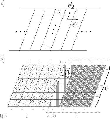
Figure 3: A ribbon infinite in $\vec{e}_{1}$ direction with $N_{2}$ unit cells in $\vec{e}_{2}$-direction (a). Nonzero polarization $\vec{P}$ implies end charge $Q^{\text{e}}$ once the ribbon is terminated (b). The end charge $Q^{\text{e}}$, defined as the charge contained in the region bounded by the dashed lines, can be computed by multiplying the charge density $\rho$ in Eq. (9) by continuous ramp function $f_{1}(r_{1})$, which takes values $0$ (dotted region), $r_{1}-r_{01}$ (hatched region) and $1$ (filled region) (b), followed by integration over the whole space. The region where the ramp function takes non-zero values is denoted by dashed line $(\vec{r}-{\vec{r}}_{0})\cdot\vec{n}=0$, which crosses the ribbon far from ends.

For purposes of this work, we will be interested in polarization of a ribbon. Consider a ribbon infinite in the $\vec{e}_{1}$ direction, with $N_{2}$ unit cells in the $\vec{e}_{2}$ direction, where $\vec{e}_{1,2}$ are lattice vectors; see Fig. 3a. We assume that the ribbon is described by a gapped $(NN_{2})\times(NN_{2})$ Bloch Hamiltonian $h_{k_{1}}$, where $N$ is the number of sites per unit cell. For each $k_{1}$ point, we denote the projector onto occupied Bloch wavefunctions $|\psi_{nk_{1}}\rangle$ by ${\cal P}_{k_{1}}=\sum_{n=1}^{N_{2}N_{\text{occ}}}|\psi_{nk_{1}}\rangle\langle\psi_{nk_{1}}|$, where the integer $N_{\text{occ}}$ is the number of the occupied states per unit cell. For the definition of ${\cal P}_{k_{1}}$, the scalar product is assumed to be taken over the supercell only, i.e., ${\cal P}_{k_{1}}$ is $(NN_{2})\times(NN_{2})$ matrix and ${\cal P}_{k_{1}+2\pi}={\cal P}_{k_{1}}$. Modern theory of electric polarization states that the polarization $\vec{P}$ of the ribbon is given by King-Smith and Vanderbilt (1993); Rhim et al. (2017)

$$\vec{P}= \frac{e}{2\pi}\left(i\ln{\det}^{\prime}\left[\prod_{k_{1}}{\cal P}_{k_{1}}\right]\vec{e}_{1}-\int_{0}^{2\pi}dk_{1}\text{Tr}\left[\vec{\hat{x}}{\cal P}_{k_{1}}\right]\right),$$ (16)

where ${\det}^{\prime}U$ denotes the product of non zero eigenvalues of $U$ and $\vec{\hat{x}}$ is the position operator. The polarization (16) depends on the choice of the origin ${\vec{r}}=0$, which can be avoided if the above expression is modified to include the ionic contribution to the charge density. The bulk-boundary correspondence states

$$Q^{\text{e}}\mod e =L\vec{P}\cdot\vec{n}/|\vec{e}\times\vec{e}_{1}|,$$ (17)

where $\vec{n}$ is a unit vector, perpendicular to some lattice vector $\vec{e}$, and $L=|\vec{e}|$ is the shortest repeated length along the direction $\vec{e}$. The end charge $Q^{\text{e}}$, which is the macroscopic charge contained in the dashed region in Fig. 3b, can be computed from Eq. (9).

An alternative formulation of electric polarization is obtained by expressing the projector (6) onto the occupied states of the ribbon as

$${\cal P}=\sum_{R_{1}}{\cal P}_{R_{1}}=\sum_{R_{1},n}|w_{R_{1},n}\rangle\langle w_{R_{1},n}|,$$ (18)

where $|w_{R_{1},n}\rangle$ are (nonunique) exponentially localized Wannier functions (WFs) and $R_{1}$ enumerates different supercells of the ribbon. When the ribbon is infinite (or under periodic boundary conditions), the shape of WFs is independent of $R_{1}$ due to translational symmetry. The polarization (16) can be expressed using WFs as

$$\vec{P} =-e\mathrm{Tr}\left[{\cal P}_{R_{1}}\vec{\hat{x}}\right]\mod e\vec{e}_{1},$$ (19)

which is independent of $R_{1}$.

III Bulk-and-edge to corner correspondence

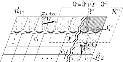
Figure 4: A charge neutral flake with total bulk polarization zero. The flake is semi-infinite in both directions. Two cuts (wavy lines) along a charge neutral lines $({\vec{r}}-{\vec{r}}_{0})\cdot\vec{n}_{\alpha}=0$, $\alpha=1,2$, split the flake into four subsystems: the two edges (dotted regions), the corner (hatched region) and the remaining bulk subsystem. A fractional part of the upper-right corner charge is given by Eq. (20). If the cuts are chosen to be Wannier cuts, the resulting polarization of the edge subsystem is called Wanner edge polarization $\vec{\mathfrak{P}}^{\text{edge}}_{\alpha}$. The corner region ${\cal R}^{\text{c}}$ is enclosed by dashed line. The end charge of the two edge subsystems is denoted by $Q^{\text{e1}}$ and $Q^{\text{e2}}$.

In this section, we prove the correspondence (4) between the corner charge and the bulk-and-edge. We consider a terminated system (flake) with vanishing bulk polarization and focus on the upper-right corner, where for the purpose of the following discussion we may assume that the remaining three corners lie at infinity. We use the notation where two edges have unit normal vectors $\vec{n}_{\alpha}$ and are along certain lattice vectors $\vec{e}_{\alpha}$, $\alpha=1,2$. The lattice vectors ${\vec{e}}_{1}$ and ${\vec{e}}_{2}$ define the unit-cell area $A_{\text{cell}}=|\vec{e}_{1}\times\vec{e}_{2}|$; see Fig. 4. The reduced coordinates $(r_{1},r_{2})$ are defined as ${\vec{r}}=r_{1}{\vec{e}}_{1}+r_{2}{\vec{e}}_{2}$.

We make two cuts along the lines $({\vec{r}}-{\vec{r}}_{0})\cdot\vec{n}_{\alpha}=0$, where the point ${\vec{r}}_{0}$ lies in the bulk. These cuts divide the flake into four regions (subsystems) (see Fig. 4): the two half-infinite edges (dotted regions), the corner (hatched region), and the remaining bulk region. Denoting the corner charge of the bulk subsystem by $\bar{Q}^{\text{c}}$, we express the flake’s corner charge $Q^{\text{c}}$ as

$$Q^{\text{c}} =\bar{Q}^{\text{c}}+Q^{\text{e}1}+Q^{\text{e}2}\mod e,$$ (20)

where $Q^{\text{e}1,2}$ are the end charges of the two edge subsystems; see Fig. 4. In writing above relation, we used that the corner-subsystem is charge neutral. (More generally, it contains integer multiple of electron charge $e$.)

While many cuts allow one to separate flake into four subsystems, we additionally require that $\bar{Q}^{\text{c}}$ is a bulk quantity and $\vec{\mathfrak{P}}^{\text{edge}}_{\alpha}$ are edge quantities. To be more precise, we require that $\bar{Q}^{\text{c}}$ is computable in terms of the bulk band structure, and similarly $\vec{\mathfrak{P}}^{\text{edge}}_{\alpha}$ should be computable from the ribbon band structure for the ribbon along $\vec{e}_{\alpha}$. We call such cuts Wannier cuts, and the resulting edge polarizations $\vec{\mathfrak{P}}^{\text{edge}}_{\alpha}$ Wannier edge polarizations. For a Wannier cut, the relation (20) becomes bulk-and-edge to corner correspondence,

$$Q^{\text{c}} =\bar{Q}^{\text{c}}+\frac{L_{2}}{A_{\text{cell}}}\vec{\mathfrak{P}}_{1}^{\text{edge}}\cdot\vec{n}_{2}+\frac{L_{1}}{A_{\text{cell}}}\vec{\mathfrak{P}}_{2}^{\text{edge}}\cdot\vec{n}_{1}\mod e.$$ (21)

Below we first define the bulk subsystem and prove that the resulting $\bar{Q}^{\text{c}}$ is expressed in terms of quadrupole tensor of the charge density of the Wannier functions. Subsection III.2 details on how to compute Wannier edge polarization $\vec{\mathfrak{P}}^{\text{edge}}_{\alpha}$.

III.1 Bulk-subsystem.

To define the bulk subsystem, we make a choice for bulk WFs, $\bar{w}_{\vec{R}n}(\vec{x})$. Assuming that WFs are assigned to their home unit cell, the charge density of the bulk WFs $\rho^{\text{WF}}({\vec{r}})$, centered around ${\vec{r}}=0$, reads

$$\rho^{\text{WF}}(\vec{r}-\vec{R}) =-e\sum_{{\vec{x}}n}|\bar{w}_{\vec{R}n}(\vec{x})|^{2}\delta(\vec{r}-\vec{x})+\rho_{\vec{R}}^{\text{ion}}(\vec{r}),$$ (22)

where we included the ionic contribution $\rho^{\text{ion}}_{\vec{R}}$ to the unit cell at $\vec{R}$. The second moment of the above charge density defines the (bulk) quadrupole tensor density $\hat{q}$,

$$\hat{q} =\frac{1}{A_{\text{cell}}}\sum_{\alpha,\beta=1,2}\hat{q}_{\alpha\beta}\vec{e}_{\alpha}\otimes\vec{e}_{\beta},$$ (23)

where “$\otimes$” denotes tensor product and $\hat{q}_{\alpha\beta}=\langle r_{\alpha}r_{\beta}\rangle_{\rho^{\text{WF}}}\equiv\int d^{2}r\rho^{\text{WF}}({\vec{r}})r_{\alpha}r_{\beta}$.

We now go back to the flake from Fig. 4, and select the rectangle $\square$ in the reduced coordinates $(r_{1},r_{2})$. We define the bulk subsystem to consist of the flake’s WFs with the center in the rectangle $\square$; see Fig. 5. For the rectangle $\square$ deep in the bulk, the bulk-subsystem is obtained by tiling the rectangle $\square$ with the bulk WFs. Hence, its charge density $\bar{\rho}(\vec{x})$ takes a simple form:

$$\bar{\rho}(\vec{r})= \sum_{\vec{R}\in\square}\rho^{\text{WF}}(\vec{r}-\vec{R}).$$ (24)

Note that the charge density $\bar{\rho}$ extends beyond the rectangle $\square$.

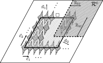
Figure 5: A flake with the regions $\square$ (dotted region with a thick solid line) and ${\cal R}^{\text{c}}$ (hatched region with dashed line). The bulk subsystem, located away from the edges (thin solid lines), is obtained by tiling $\square$ with the occupied bulk WFs (wavy star-shaped objects). The integer $R_{\text{WF}}$ is the “radius” of the bulk WFs, outside of it the charge density of the bulk WFs can be neglected.

We now prove that the corner charge and the edge dipole of the bulk subsystem, $\bar{Q}^{\text{c}}_{\alpha}$ and $\bar{D}^{\text{edge}}_{\alpha}$, are expressed in terms of the bulk quadrupole tensor $\hat{q}$. For simplicity, we assume that all sites of the flake lie on the lattice itself (lattice without the basis). In this case, instead of working with $\rho^{\text{WF}}({\vec{r}})$, we use the quantity $Q^{\text{WF}}_{\vec{R}}$: the charge at lattice position $\vec{R}$, originating from the bulk Wannier functions centered at $\vec{R}=0$,

$$Q^{\text{WF}}_{\vec{R}} =-e\sum_{n=1}^{N_{\text{occ}}}|w_{(0,0)n}(\vec{R})|^{2}+N_{\text{occ}}e\delta_{R_{1},0}\delta_{R_{2},0}.$$ (25)

In the above expression, we assume that the ionic charge contribution $eN_{\text{occ}}$ is localized at the lattice sites, and thus $\sum_{\vec{R}}Q^{\text{WF}}_{\vec{R}}=0$. We compute $\bar{Q}^{\text{c}}$ using the corner region ${\cal R}^{\text{c}}$ with boundaries $({\vec{r}}-{\vec{r}}_{0})\cdot\vec{n}_{\alpha}=0$, where ${\vec{r}}_{0}$ lies in the bulk; see Fig. 5. Hence, the corner charge of the bulk subsystem $\bar{Q}^{\text{c}}$ is obtained from Eq. (14),

$$\bar{Q}^{\text{c}}=\sum_{\vec{R}\in\square} \left[-\theta(-R_{1})R_{\text{WF}}-\theta(-R_{2})R_{\text{WF}}+\theta(-R_{1})\theta(-R_{2})\right.$$

$$+\theta(R_{1})(R_{\text{WF}}-\theta(-R_{2}))+\theta(R_{2})(R_{\text{WF}}-\theta(-R_{1}))$$

$$\left.+\theta(R_{1})\theta(R_{2})\right]Q^{\text{WF}}_{\vec{R}},$$ (26)

where $\theta(x)\equiv|x|H(x)$ with $H(x)$ being the Heaviside step function and $R_{\text{WF}}$ being the radius of the bulk WFs, see Fig. 5. Since $\sum_{\vec{R}}Q^{\text{WF}}_{\vec{R}}=0$ holds, only the bulk WFs whose charge is not fully contained in ${\cal R}^{\text{c}}$ contribute to $\bar{Q}^{\text{c}}$. The three terms in the first line of the sum (26) count the charge contained in the region outside of ${\cal R}^{\text{c}}$ (not necessarily inside of $\square$), originating from the bulk WFs whose center is in ${\cal R}^{\text{c}}$. Similarly, the second and the third lines of the sum (26) correspond to the charge contained within ${\cal R}^{\text{c}}$, originating from the bulk WFs whose center is in $\square\setminus{\cal R}^{\text{c}}$. Using the assumption that the bulk polarization vanishes $\vec{P}=\sum_{\vec{R}}\vec{R}Q^{\text{WF}}_{\vec{R}}=0$, we rewrite Eq (26) as

$$\bar{Q}^{\text{c}} =\sum_{\vec{R}\in\square}R_{1}R_{2}Q^{\text{WF}}_{\vec{R}}=\frac{L_{1}L_{2}}{A_{\text{cell}}}\vec{n}_{1}\cdot\hat{q}\cdot\vec{n}_{2},$$ (27)

where in the last equality we used Eq. (23), $L_{\alpha}=|\vec{e}_{\alpha}|$, and that the unit normal vectors $\vec{n}_{\alpha}$ point toward the outside of the subsystem. The above result is valid for both convex and concave angles $\angle(\vec{e}_{1},\vec{e}_{2})$.

To obtain the edge dipole $\bar{D}^{\text{edge}}_{1}$ from the charge density $\bar{\rho}$, we consider a flake infinite in the $\vec{e}_{1}$ direction (ribbon) and focus on the upper edge. For concreteness we assume that the unit cells at the top edge of $\square$ have coordinates $(R_{1},-1)$. Because of translational invariance, the charge $\mathfrak{Q}_{R_{2}}$, which is (microscopic) charge of the ribbon at the lattice site $\vec{R}$, is independent of $R_{1}$. Using Eqs. (24) and (25) we write,

$$\mathfrak{Q}_{R_{2}} =\begin{cases}\sum_{R_{2}^{\prime}>R_{2}}Q^{\text{WF}}_{R_{2}^{\prime}}&R_{2}\geq 0,\\ -\sum_{R_{2}^{\prime}\leq R_{2}}Q^{\text{WF}}_{R_{2}^{\prime}}&R_{2}<0,\end{cases}$$ (28)

where the notation $Q^{\text{WF}}_{R_{2}}\equiv\sum_{R_{1}}Q^{\text{WF}}_{\vec{R}}$ has been introduced. The edge dipole [see Eq. (13)] for the edge along $\vec{e}_{1}$ is expressed as

$$\frac{\bar{D}^{\text{edge}}_{1}}{{\vec{e}}_{2}\cdot\vec{n}_{1}} =\sum_{R_{2}}R_{2}\mathfrak{Q}_{R_{2}}$$

$$=-\sum_{R_{2}\geq 0}R_{2}\sum_{-R_{2}<R_{2}^{\prime}\leq R_{2}}Q^{\text{WF}}_{R_{2}^{\prime}}.$$ (29)

Changing the order of the two sums in the above expression, we obtain

$$\frac{\bar{D}^{\text{edge}}_{1}}{{\vec{e}}_{2}\cdot\vec{n}_{1}}= \sum_{R_{2}^{\prime}\geq 0}Q^{\text{WF}}_{R_{2}^{\prime}}\sum_{R_{2}^{\prime}\leq R_{2}<R_{\text{WF}}}R_{2}-\sum_{R_{2}^{\prime}<0}Q^{\text{WF}}_{R_{2}^{\prime}}\sum_{R_{2}^{\prime}\leq R_{2}<R_{\text{WF}}}R_{2}$$

$$=\frac{1}{2}\sum_{R_{2}^{\prime}}{R_{2}^{\prime}}^{2}Q^{\text{WF}}_{R_{2}^{\prime}},$$ (30)

where the cutoff $R_{\text{WF}}$ drops out for the ribbon wider than the radius of the bulk WFs, and in writing the second line we used $\sum_{R_{2}^{\prime}}Q^{\text{WF}}_{R_{2}^{\prime}}=\sum_{R_{2}^{\prime}}R_{2}^{\prime}Q^{\text{WF}}_{R_{2}^{\prime}}=0$. Repeating the same calculation for the other edge, we obtain

$$\bar{D}^{\text{edge}}_{\alpha}=L_{\alpha}\vec{n}_{\alpha}\cdot\hat{q}\cdot\vec{n}_{\alpha}/2.$$ (31)

Figure 6: A corner defined by the edges along lattice vectors ${\vec{e}}_{1,2}$ and unit-normal vectors $\vec{n}_{1,2}$. The corner region ${\cal R}^{\text{c}}$ is defined by the (dashed) lines $({\vec{r}}-{\vec{r}}_{0})\cdot\vec{n}_{\alpha}^{\prime}=0$, where the point ${\vec{r}}_{0}$ lies in the bulk.

The relations (27) and (31) show that the corner charge and the edge dipole resulting from the macroscopic average of the charge density $\bar{\rho}$, can be seen to be be generated by polarizations $L_{\alpha}\hat{q}\cdot\vec{n}_{\alpha}/2$, placed long the four edges of $\square$. For a more general case, when the corner region ${\cal R}^{\text{c}}$ is defined by lines $({\vec{r}}-{\vec{r}}_{0})\cdot\vec{n}_{\alpha}^{\prime}=0$, applying the bulk-boundary correspondence (17) to these edge polarizations gives

$$\bar{Q}^{\text{c}} =\frac{L_{1}|\vec{e}_{2}^{\prime}|}{|\vec{e}_{1}\times\vec{e}_{2}^{\prime}|}\vec{n}_{2}^{\prime}\cdot\hat{q}\cdot\vec{n}_{1}/2+\frac{|\vec{e}_{1}^{\prime}|L_{2}}{|\vec{e}_{1}^{\prime}\times\vec{e}_{2}|}\vec{n}_{1}^{\prime}\cdot\hat{q}\cdot\vec{n}_{2}/2,$$ (32)

where $\vec{e}_{\alpha}^{\prime}$ are lattice vectors satisfying $\vec{e}_{\alpha}^{\prime}\cdot\vec{n}_{\alpha}^{\prime}=0$, normalized such that $|\vec{e}_{\alpha}^{\prime}|$ gives the shortest repeated length in the lattice direction $\vec{e}_{\alpha}^{\prime}$, see Fig. 6. The above expression reduces to Eq. (27) for $\vec{n}_{\alpha}^{\prime}=\vec{n}_{\alpha}$.

III.2 Edge-subsystem. Wannier edge polarization $\vec{\mathfrak{P}}_{\alpha}^{\text{edge}}$.

To define the edge subsystem and Wannier edge polarization, we considering a ribbon with the periodic boundary condition in the $\vec{e}_{\alpha}$ direction. We call “Wannier cut” the procedure where the bulk Wannier functions, used to define the bulk subsystem in the previous subsection, are removed from the middle of the ribbon. After such removal, what remains of the ribbon are two edge subsystems. For a sufficiently wide cut, the charge densities of the two edge subsystems do not overlap when projected onto the ${\vec{e}}_{\bar{\alpha}}$ direction. Therefore, we can define the subsystem corresponding to a single edge $\alpha$ and its polarization we call Wannier edge polarization $\vec{\mathfrak{P}}_{\alpha}^{\text{edge}}$.

For concreteness, we set $\alpha=1$ and denote by $h_{k_{1}}$ the Bloch Hamiltonian of the ribbon, with supercell having $2N_{2}+1$ unit cells located at positions $R_{2}\vec{e}_{2}$, $R_{2}\in[-N_{2},N_{2}]$. The translationally invariant Wannier cut is performed using hybrid bulk WFs $|\bar{w}_{k_{1}R_{2}n}\rangle$,

$$|\bar{w}_{k_{1}R_{2}n}\rangle =\sum_{R_{1}=-N_{1}}^{N_{1}-1}e^{ik_{1}R_{1}}|\bar{w}_{\vec{R}n}\rangle,$$ (33)

where the periodic boundary condition identifies the sites at $R_{1}=-N_{1}$ with those at $R_{1}=N_{1}$. The Wannier cut is performed in the middle of the ribbon supercell by removing $2L+1$ hybrid bulk WFs $|\bar{w}_{k_{1}R_{2}n}\rangle$ with $R_{2}\in[-L,L]$ from the space spanned by the occupied states

$${\cal P}_{k_{1}}^{L} \equiv{\cal P}_{k_{1}}-\sum_{\begin{subarray}{c}n=1\\ R_{2}=-L\end{subarray}}^{\begin{subarray}{c}n=N_{\text{occ}}\\ R_{2}=L\end{subarray}}|\bar{w}_{k_{1}R_{2}n}\rangle\langle\bar{w}_{k_{1}R_{2}n}|.$$ (34)

The integer $L$ should be chosen sufficiently large such the projector $P_{k_{1}}^{L}$ does not contain the sites from the middle unit cell of the supercell, i.e.,

$${\cal P}_{k_{1}}(\vec{x},\vec{x}^{\prime})\rightarrow 0,$$ (35)

for the reduced coordinates $x_{2},x_{2}^{\prime}\in[-1/2,1/2]$. As WFs are more localized, a smaller value of $L$ is required. The matrix elements of the projector onto occupied states of the edge subsystem above the Wannier cut read

$${\cal P}^{\text{edge}}_{k_{1}}(\vec{x},\vec{x}^{\prime}) =H(x_{2})H(x_{2}^{\prime}){\cal P}_{k_{1}}^{L}(\vec{x},\vec{x}^{\prime}).$$ (36)

Note that for a ribbon with the fixed width $N_{2}$, the value of $L$ should not be too large; otherwise the hybrid bulk WFs do not fully belong to the space of occupied states of the ribbon. This can be diagnosed by inspecting the charge neutrality of the resulting edge subsystem’s supercell,

$$\sum_{\vec{x}}\int\frac{dk_{1}}{2\pi}{\cal P}^{\text{edge}}_{k_{1}}(\vec{x},\vec{x})\rightarrow N_{\text{occ}}(N_{2}-L),$$ (37)

where the value on the right-hand side is the ionic charge—the removal of the hybrid bulk WF also removes the corresponding ionic charge. If the conditions (35) and (37) are satisfied with required accuracy, the Wannier cut has been performed successfully. The edge polarization $\vec{\mathfrak{P}}^{\text{edge}}_{1}$ is given by Eq. (16) using ${\cal P}^{\text{edge}}_{k_{1}}$ in place of ${\cal P}_{k_{1}}$.

III.3 Discussion

Putting together the bulk and the edge subsystems, we obtain the main result of our work, namely that the corner charges and the edge dipoles are determined by the edge polarizations (3). The bulk-and-edge to corner charge correspondence is obtained after substituting Eq. (32) and the expression for the edge polarization into Eq. (20),

$$Q^{\text{c}}_{{\cal R}^{\text{c}}} =\frac{|\vec{e}_{2}^{\prime}|}{|\vec{e}_{2}^{\prime}\times\vec{e}_{1}|}\vec{P}^{\text{edge}}_{1}\cdot\vec{n}_{2}^{\prime}+\frac{|\vec{e}_{1}^{\prime}|}{|\vec{e}_{1}^{\prime}\times\vec{e}_{2}|}\vec{P}^{\text{edge}}_{2}\cdot\vec{n}_{1}^{\prime},$$ (38)

where the corner charge is defined by the corner region ${\cal R}^{\text{c}}$ in Fig. 6. It is worth mentioning that not only Wannier polarization $\vec{\mathfrak{P}}^{\text{edge}}_{\alpha}$ but also the edge polarization (3) depends on the choice of the bulk WFs. This observation agrees with the previously mentioned statement that the two edge polarizations $\vec{P}^{\text{edge}}_{\alpha}$ have four independent components whereas there are only three independent physical observables.

The bulk subsystem defined in Sec. III.1 is special because its charge density can be obtained by tiling. The bulk subsystem can be viewed as a flake with a special termination that we call Wannier termination. It is instructive to compare the relation between the corner charge and the quadrupole moment of a flake with an arbitrary termination versus the one with Wannier termination. Assuming that the two lowest moments of the flake’s (microscopic) charge density $\rho^{\text{flake}}$ vanish, we write the second (off-diagonal) moment as

$$\hat{q}^{\text{flake}}_{12} =\frac{1}{N_{1}N_{2}A_{\text{cell}}}\langle x_{1}x_{2}\rangle_{\rho^{\text{flake}}},$$ (39)

where the flake has $N_{1,2}$ unit cells along the two primitive vectors. For an inversion-symmetric rhomboid flake, the macroscopic charge density $\rho^{\text{flake},\text{macro}}$ consists of four corner charges $Q^{\text{c}}$ with alternating signs superimposed with the edge dipoles, see Sec. II.1. Denoting the coordinates of the center of charge of the top-right corner by $\vec{X}=\frac{1}{2}X_{1}\vec{e}_{1}+\frac{1}{2}X_{2}\vec{e}_{2}$, with the origin at the flake’s inversion center, gives $\langle x_{1}x_{2}\rangle_{\rho^{\text{flake},\text{macro}}}=\langle x_{1}x_{2}\rangle_{\rho^{\text{flake}}}=Q^{\text{c}}X_{1}X_{2}$. The corner charge $Q^{\text{c}}$ can be approximated from the flake’s quadrupole moment,

$$Q^{\text{c}} \sim\frac{X_{1}X_{2}}{N_{1}N_{2}}Q^{\text{c}}=\frac{L_{1}L_{2}}{A_{\text{cell}}}\vec{n}_{1}\cdot\hat{q}^{\text{flake}}\cdot\vec{n}_{2}.$$ (40)

We used that $X_{\alpha}/N_{\alpha}\rightarrow 1$ in the thermodynamic limit $N_{\alpha}\rightarrow\infty$. Hence, for a flake with an arbitrary termination, the corner charge can be obtained from the microscopic charge density $\rho^{\text{flake}}$ from Eqs. (39) and (40) only with algebraic accuracy in the flake’s size. On the other hand, for a flake with Wannier termination (i.e., bulk subsystem), $\hat{q}^{\text{flake}}$ is given by Eq. (23), and we know that the relation (27) holds with exponential accuracy as the flake size is increased beyond the radius of the tile (Wannier functions). In other words, Wannier termination pins $X_{1}$ ($X_{2}$) to the value $N_{1}$ ($N_{2}$).

IV Examples

In this section, we consider three two-dimensional tight-binding models which we use to illustrate the procedure described in the previous section. For each example, we perform two independent calculations: (1) After diagonalization of the flake’s Hamiltonian, we obtain macroscopic charge density $\rho^{\text{macro}}$ from Eqs. (5) and (7), and subsequently the corner charge $Q^{\text{c}}$ and the edge dipole $D^{\text{edge}}$ from Eqs. (12) and (11), and (2) we make a choice of the occupied bulk WF, calculate the bulk quadrupole tensor and the Wannier edge polarizations for each edge of interest—these quantities give the edge polarization (3) that are used to compute the corner charge and the edge dipole moments; see Eqs. (4) and (15). Alternatively, $D^{\text{edge}}_{\alpha}$ can be obtained from the corresponding ribbon calculation, see Eq. (13). The first example considers the Benalcazar-Bernevig-Hughes (BBH) model Benalcazar et al. (2017, 2019) with broken fourfold rotation symmetry such that the corner charge is no longer quantized. In the dimerized limit of BBH model, the procedure from Sec. III is carried out analytically. The second example considers a model with a single occupied band where the corners are formed by several different orientations of the edges. The final example is meant to illustrate a scenario where the bulk contribution to the edge polarization (3) is small, which explains why it was overlooked in Ref. Zhou et al., 2015.

To carry out the above-mentioned calculations, we need to specify the bulk Hamiltonian and the edge boundary conditions. We consider a special form of boundary conditions that we call “theorist” boundary conditions: The Hamiltonian around the boundaries is assumed to be the same as the bulk Hamiltonian with the hoppings to the missing sites set to zero. Theorist boundary conditions are used here out of convenience; they do not have any particular relevance for realistic systems.

IV.1 BBH model with broken fourfold rotation symmetry

Here we consider a two-dimensional $\pi$-flux dimerized model, Benalcazar et al. (2017, 2019) which is a particular case of BBH model that exhibits quantized corner charge protected by fourfold rotation symmetry ${\cal C}_{4}$

$$H= e^{i\pi/4}\sum_{{\vec{R}}}\left(|{\vec{R}},1\rangle\langle{\vec{R}}+{\vec{a}}_{x},2|+|{\vec{R}}+{\vec{a}}_{y},4\rangle\langle{\vec{R}},1|\right.$$

$$+|{\vec{R}}+{\vec{a}}_{x}+{\vec{a}}_{y},3\rangle\langle{\vec{R}}+{\vec{a}}_{y},4|$$

$$\left.+|{\vec{R}}+{\vec{a}}_{x},2\rangle\langle{\vec{R}}+{\vec{a}}_{x}+{\vec{a}}_{y},3|\right)+\text{h.c.}+H_{4},$$ (41)

where the four orbitals $|{\vec{R}}\gamma\rangle$, $\gamma=1,\dots,4$ are placed on a square lattice with primitive vectors ${\vec{a}}_{\alpha}=a{\vec{e}}_{\alpha}$, where ${\vec{e}}_{x}$ (${\vec{e}}_{y}$) is the unit vector along the $x$ ($y$) direction. The fourfold rotation acts as ${\cal C}_{4}:|{\vec{R}}\gamma\rangle\rightarrow|{\vec{R}}\gamma+1\rangle$ and is responsible for the quantization Benalcazar et al. (2019) of the corner charge to the value of $Q^{\text{c}}=e/2\mod e$. The term $H_{4}$ breaks fourfold rotation symmetry while preserving its twofold rotation subgroup

$$H_{4}=\delta\sum_{\vec{R}}(-1)^{\gamma}|{\vec{R}}\gamma\rangle\langle{\vec{R}}\gamma|.$$ (42)

The two occupied bulk Wannier functions localized on four sites can be written as

$$\bar{w}_{{\vec{R}}1} =\left(\frac{\sqrt{2+\delta_{+}^{2}}}{\sqrt{2+\delta^{2}}},-\frac{e^{3i\pi/4}}{\sqrt{2+\delta_{+}^{2}}},0,\frac{e^{i\pi/4}}{\sqrt{2+\delta_{+}^{2}}}\right)^{T},$$

$$\bar{w}_{{\vec{R}}2} =\left(0,\frac{\sqrt{1+\frac{\delta_{-}^{2}}{2}}}{2\sqrt{2+\delta^{2}}},\frac{e^{-i\pi/4}}{\sqrt{1+\frac{\delta_{-}^{2}}{2}}},\frac{i\sqrt{1+\frac{\delta_{-}^{2}}{2}}}{2\sqrt{2+\delta^{2}}}\right)^{T},$$ (43)

where the basis for the spinor is $\{|{\vec{R}},1\rangle,|{\vec{R}}+{\vec{a}}_{x},2\rangle,|{\vec{R}}+{\vec{a}}_{x}+{\vec{a}}_{y},3\rangle,|{\vec{R}}+{\vec{a}}_{y},4\rangle\}$, and the notation $\delta_{\pm}=\delta\pm\sqrt{2+\delta^{2}}$ is used. The above bulk Wannier functions give the following components of the bulk quadrupole tensor (23)

$$\hat{q}_{xy} =\frac{e}{1+\delta_{-}^{2}/2}\mod e,$$

$$\hat{q}_{xx} =\hat{q}_{yy}=0\mod e.$$ (44)

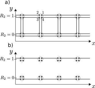
Figure 7: The ribbon corresponding to the BBH model (41) with theorist boundary conditions in the $y$ direction. The bulk Wannier functions can be chosen to be localized on four sites and are represented by the squares (a). The projector ${\cal P}^{L=1}_{k_{x}}$ is obtain by removing the bulk Wannier functions belonging to the unit cell at $R_{2}=0$ (b); see Eq. (34). Dashed circles group the sites that belong to the same unit cell and integers correspond to $\gamma$.

Wannier edge polarization $\vec{\mathfrak{P}}_{x}$ is computed by considering ribbon with theorist boundary conditions in the $y$ direction. We take the ribbon supercell to consist of two unit cells (eight sites) with coordinates $R_{y}=0,1$; see Fig. 7. The projector ${\cal P}^{L=1}_{k_{x}}$ onto the ribbon states after performing Wannier cut, which removes the hybrid bulk WFs with $R_{2}=0$ [see Eq. (34)], reads

$${\cal P}_{k_{x}}^{L=1} =\begin{pmatrix}|\psi^{\text{edge}}_{k_{x}}\rangle\langle\psi^{\text{edge}}_{k_{x}}|&0_{2\times 4}&0_{2\times 2}\\ 0_{4\times 2}&0_{4\times 4}&0_{4\times 2}\\ 0_{2\times 2}&0_{2\times 4}&|\psi^{\text{edge'}}_{k_{x}}\rangle\langle\psi^{\text{edge'}}_{k_{x}}|\end{pmatrix},$$

$$|\psi^{\text{edge}}_{k_{x}}\rangle =\left(\frac{\tilde{\delta}_{+}}{\sqrt{1+\tilde{\delta}_{+}^{2}}},-\frac{e^{-i\pi/4e^{ik_{x}a}}}{\sqrt{1+\tilde{\delta}_{+}^{2}}}\right)^{T},$$ (45)

where $\tilde{\delta}_{+}=\delta+\sqrt{1+\delta^{2}}$ and $|\psi^{\text{edge'}}_{k_{x}}\rangle={\cal C}_{4}^{2}|\psi^{\text{edge}}_{-k_{x}}\rangle$; see Fig. 7b. Taking the corresponding subblock of the matrix ${\cal P}_{k_{x}}^{L=1}$ [see Eq. (36)] gives the projector onto the upper edge subsystem

$${\cal P}_{k_{x}}^{\text{edge}} =\begin{pmatrix}|\psi^{\text{edge}}_{k_{x}}\rangle\langle\psi^{\text{edge}}_{k_{x}}|&0_{2\times 2}\\ 0_{2\times 2}&0_{2\times 2}\end{pmatrix}.$$ (46)

Repeating the same calculation for the ribbon along the $y$ direction, after substituting ${\cal P}_{k_{x}}^{\text{edge}}$ (${\cal P}_{k_{y}}^{\text{edge}}$) into Eq. (16), we obtain the two Wannier edge polarizations,

$$\vec{\mathfrak{P}}^{\text{edge}}_{\alpha} =\frac{ae}{1+\tilde{\delta}_{+}^{2}}{\vec{e}}_{\alpha}.$$ (47)

The edge polarizations (3) read

$$\vec{P}^{\text{edge}}_{\alpha} =\left(\frac{1}{1+\tilde{\delta}_{+}^{2}}+\frac{1}{2+\delta_{-}^{2}}\right)ae{\vec{e}}_{\alpha}.$$ (48)

The above result implies that the edge dipoles vanish $D^{\text{edge}}_{\alpha}=0$, while the corner charge of the upper-right corner $Q^{\text{c}}$ reads

$$Q^{\text{c}} =\frac{2e}{1+\tilde{\delta}_{+}^{2}}+\frac{e}{1+\delta_{-}^{2}/2}\mod e.$$ (49)

Alternatively, considering the flake with theorist boundary conditions in both $x$ and $y$ directions, the corner charge $Q^{\text{c}}$ can be computed via Eq. (14), which agrees with the result (49).

IV.2 Orbitals without internal quadrupole moment

This example considers a two-dimensional tight-binding model with two sites per unit cell, defined on an arbitrary Bravais lattice with primitive vectors $\vec{a}_{1}$ and $\vec{a}_{2}$. The Hamiltonian is written as

$$h= \sum_{\vec{R}}\left[\sum_{\gamma=1,2}\left((-1)^{\gamma}\delta|\vec{R}\gamma\rangle\langle\vec{R}\gamma|\right.\right.$$ (50)

$$\left.\left.+\sum_{d=1,2}((-1)^{\gamma}t|\vec{R}\gamma\rangle\langle\vec{R}+\vec{a}_{d}\bar{\gamma}|+t_{\gamma}|\vec{R}\gamma\rangle\langle\vec{R}+\vec{a}_{d}\gamma|)\right)\right],$$

where $|\vec{R}\gamma\rangle$ is the $\gamma$ orbital at the position $\vec{R}$ and $\{\bar{1},\bar{2}\}=\{2,1\}$. The above Hamiltonian has inversion symmetry that maps the $\gamma$ orbital into itself; hence the bulk polarization is quantized. We make a choice of parameters of Hamiltonian (50) such that the bulk is gapped at half-filling and for theorist boundary conditions the corner charge is sizable, $\delta=-1$, $t=-0.08$, $t_{1}=3.5\times t$, and $t_{2}=-1.5\times t$. It is easy to see that for these parameters, the bulk polarization vanishes.

Figure 8: Three different corners for the system described by the Hamiltonian (50) with the corresponding corner regions (dashed lines). The corner between the edges along the primitive vectors $\vec{a}_{1}$ and $\vec{a}_{2}$, with the corner region parallel to the edges (a). The corner defined by the lattice vectors $\vec{e}_{1}=2\vec{a}_{1}+\vec{a}_{2}$ and $\vec{a}_{2}$ (b)-(c). Choosing the corner region above the line along $\vec{a}_{1}$ (b) results in a different corner charge compared to the corner region parallel to the edges (c), i.e., $Q^{\text{c}}_{b}\neq Q^{\text{c}}_{c}$. The same as in panels (b) and (c) for the corner between the edges along $\vec{e}_{1}^{\prime}=2\vec{a}_{1}-\vec{a}_{2}$ and $\vec{a}_{2}$ is shown in panels (d) and (e). The unit normal vectors $\vec{n}_{1}$, $\vec{n}_{2}$ [$-\vec{n}_{2}$ for panel (e)], $\vec{n}$ and $\vec{n}^{\prime}$ are oriented to point toward the corner.

The occupied bulk WF $|\bar{w}_{\vec{R}}\rangle$ is chosen as follows. When all the hoppings are switched off $t=0$, the maximally localized WF takes the form $|\bar{w}_{\vec{R}}^{0}\rangle=|\vec{R}1\rangle$ for $\delta<0$. The corresponding (smooth) Bloch eigenfunction $|\psi_{\vec{k}}^{0}\rangle$ is given as

$$|\psi_{\vec{k}}^{0}\rangle =\langle\tilde{\psi}_{\vec{k}}|\bar{w}_{\vec{R}}^{0}\rangle|\tilde{\psi}_{\vec{k}}^{0}\rangle,$$ (51)

for $|\tilde{\psi}_{\vec{k}}^{0}\rangle$ (not necessarily smooth) Bloch eigenfunction. A smooth gauge $|\psi_{\vec{k}}^{t}\rangle$ for a finite value of the parameter $t$ is obtained by parallel transport of $|\psi_{\vec{k}}^{0}\rangle$ as the hoppings are switched on

$$|\psi_{\vec{k}}^{t}\rangle =\langle\tilde{\psi}^{t}_{\vec{k}}|\left(\prod_{t^{\prime}=0}^{t}|\tilde{\psi}_{\vec{k}}^{t^{\prime}}\rangle\langle\tilde{\psi}_{\vec{k}}^{t^{\prime}}|\right)|\psi_{\vec{k}}^{0}\rangle|\tilde{\psi}_{\vec{k}}^{t}\rangle.$$ (52)

We set $t=-0.08$ and drop the superscript $t$ from now on. The bulk WF takes the form

$$|\bar{w}_{\vec{R}}\rangle=\sum_{\vec{R}}e^{i\vec{k}\cdot\vec{R}}|\psi_{\vec{k}}\rangle.$$ (53)

Inspecting the values of $|\bar{w}_{(0,0)}(\vec{R})|^{2}$ for different unit cells, we observe that the obtained WF is well localized, with $99.5\%$ of the charge lying within the unit cell at $(0,0)$. Using Eq. (23), we obtain the bulk quadrupole tensor $\hat{q}$ with components in the $(\vec{a}_{1},\vec{a}_{2})$ basis

$$\hat{q}_{12} =\hat{q}_{21}=-1.65919\times 10^{-3}e,$$ (54)

$$\hat{q}_{11} =\hat{q}_{22}=-7.34447\times 10^{-3}e,$$ (55)

where we assumed the ion charge $e$ is localized at $\vec{R}$.

Edges along primitive vectors $\vec{a}_{1}$ and $\vec{a}_{2}$.—We now perform a ribbon calculation for a ribbon with periodic boundary conditions along the $\vec{a}_{1}$ direction and the supercell consisting of unit cells at positions $R_{2}\in-[N_{2},N_{2}]$, $N_{2}=20$. The Fourier transform of Eq. (50) gives Bloch Hamiltonian $h_{k_{1}}$. Substituting the bulk WF $|\bar{w}_{\vec{R}}\rangle$ into Eq. (33), the hybrid bulk WF $|\bar{w}_{k_{1}R_{2}}\rangle$ is obtained. We find that the projector (34) ${\cal P}_{k_{1}}^{L}$ for $L=14$ satisfies the criteria (35) and (37) both with accuracy of $10^{-12}$. From Eq. (36), the edge projector onto the top edge along $\vec{a}_{1}$, ${\cal P}^{\text{edge}}_{k_{1}}$, is obtained, giving the Wannier edge polarization

$$\vec{\mathfrak{P}}^{\text{edge}}_{\vec{a}_{1}} =(0.17609\vec{a}_{1}+3.24851\vec{a}_{2})\times 10^{-3}e,$$ (56)

where in Eq. (16) we used the grid of $120$ equally spaced $k_{1}$ points. [In this section, we index the (Wannier) edge polarizations with the corresponding edge lattice vector instead of the integer index.] The same procedure is repeated for the right edge along $\vec{a}_{2}$, which gives $\vec{\mathfrak{P}}_{\vec{a}_{2}}^{\text{edge}}$ obtained from Eq. (56) after setting $\vec{a}_{\alpha}\rightarrow\vec{a}_{\bar{\alpha}}$. Substituting Eqs. (54)-(56) into the expression for the edge polarization (3) gives

$$\vec{P}^{\text{edge}}_{\vec{a}_{\alpha}} =(-0.65350\vec{a}_{\alpha}-0.42372\vec{a}_{\bar{\alpha}})\times 10^{-3}e.$$ (57)

Edge along $\vec{e}_{1}=2\vec{a}_{1}+\vec{a}_{2}$—We consider a ribbon, periodic in $\vec{e}_{1}=2\vec{a}_{1}+\vec{a}_{2}$ direction, with supercell along $\vec{a}_{1}$-direction. Repeating the same calculation as above, we obtain for $N_{2}=30$, that choosing $L=15$ satisfies conditions (35) and (37) both with accuracy of about $10^{-8}$. The Wannier edge polarization for the upper edge of this ribbon is

$$\vec{\mathfrak{P}}^{\text{edge}}_{\vec{e}_{1}} =(6.05756\vec{e}_{1}-14.76152\vec{a}_{1})\times 10^{-3}e.$$ (58)

The above result together with Eqs. (3), (54), and (55) give the edge polarization $\vec{P}^{\text{edge}}_{\vec{e}_{1}}$ for the edge along $\vec{e}_{1}$

$$\vec{P}^{\text{edge}}_{\vec{e}_{1}} =(-0.45731\vec{e}_{1}+0.28122\vec{a}_{1})\times 10^{-3}e.$$ (59)

Edge along $\vec{e}^{\prime}_{1}=2\vec{a}_{1}-\vec{a}_{2}$—Proceeding as above, we obtain for the Wannier edge polarization for the upper edge of the ribbon along $\vec{e}^{\prime}_{1}$

$$\vec{\mathfrak{P}}^{\text{edge}}_{\vec{e}_{1}^{\prime}} =(-6.76134\vec{e}_{1}+17.14810\vec{a}_{1})\times 10^{-3}e,$$ (60)

and the corresponding edge polarization,

$$\vec{P}^{\text{edge}}_{\vec{e}_{1}^{\prime}} =(1.41273\vec{e}_{1}-4.52168\vec{a}_{1})\times 10^{-3}e.$$ (61)

Edge dipole $D^{\text{edge}}$—We confirm that relation (15) holds exactly. For example, for the edges along the lattice vectors $\vec{a}_{\alpha}$

$$\frac{\vec{P}^{\text{edge}}_{\vec{a}_{\alpha}}\cdot\vec{n}_{\alpha}}{{\vec{e}}_{\bar{\alpha}}\cdot\vec{n}_{\alpha}} =-0.42372\times 10^{-3}e,$$ (62)

agrees with the value obtained from either flake or ribbon calculation $D^{\text{edge}}_{\vec{a}_{\alpha}}/{\vec{e}}_{\bar{\alpha}}\cdot\vec{n}_{\alpha}=-0.42372\times 10^{-3}e$.

Corner charge.—Three different corners, as shown in Fig. 8, are considered. To compute the corner charge, we consider a flake with the boundaries along the edge vectors, with the lower-left corner located at $-N_{1}\vec{e}_{1}-N_{2}\vec{e}_{2}$ and the upper-right corner at $N_{1}\vec{e}_{1}+N_{2}\vec{e}_{2}$. After diagonalization of the Hamiltonian (50) for $N_{1}=N_{2}=20$, the charge density $\rho({\vec{r}})$ is obtained from Eq. (7).

For the situation in Fig. 8a, the corner charge $Q_{a}^{\text{c}}$ is obtained by integrating the charge density (7) over the corner area denoted by dashed lines; see Eq. (14). We obtain $Q_{a}^{\text{c}}=-1.30687\times 10^{-3}e$ which should be compared with Eq. (4),

$$Q^{\text{c}}_{a} =\frac{L_{2}}{A_{\text{cell}}}\vec{P}^{\text{edge}}_{\vec{a}_{1}}\cdot\vec{n}_{2}+\frac{L_{1}}{A_{\text{cell}}}\vec{P}^{\text{edge}}_{\vec{a}_{2}}\cdot\vec{n}_{1}$$

$$=-1.30700\times 10^{-3}e,$$ (63)

where $L_{\alpha}=|\vec{a}_{\alpha}|$, and $\vec{n}_{\alpha}$ is a unit normal vector as depicted in Fig. 8a.

Figures 8b and c consider the corner formed by the edges $\vec{e}_{1}=2\vec{a}_{1}+\vec{a}_{2}$ and $\vec{e}_{2}=\vec{a}_{2}$. For the corner region as in Fig. 8b, we plug the microscopic charge density (7) into Eq. (5) and use Gaussian function. The integration of macroscopic charge density over the corner region yields the corner charge $Q^{\text{c}}_{b}=-1.11059\times 10^{-3}e$ that should be compared with

$$Q^{\text{c}}_{b} =\frac{L_{1}}{A_{\text{cell}}}\vec{P}^{\text{edge}}_{\vec{e}_{1}}\cdot\vec{n}_{1}+\frac{L_{1}}{A_{\text{cell}}}\vec{P}^{\text{edge}}_{\vec{a}_{2}}\cdot\vec{n}_{1}$$

$$=-1.11081\times 10^{-3}e.$$ (64)

On the other hand, for the corner region in Fig. 8c, the corner charge $Q^{\text{c}}_{c}$ can be obtained from Eq. (14). The result $Q^{\text{c}}_{c}=-0.75998\times 10^{-3}e$ agrees well with

$$Q^{\text{c}}_{c} =\frac{L_{2}}{A_{\text{cell}}}\vec{P}^{\text{edge}}_{\vec{e}_{1}}\cdot\vec{n}_{2}+\frac{L}{A_{\text{cell}}}\vec{P}^{\text{edge}}_{\vec{a}_{2}}\cdot\vec{n}$$

$$=-0.75834\times 10^{-3}e,$$ (65)

where $L=|\vec{e}_{1}|$, and $\vec{n}$ is the unit normal vector as shown in Fig. 8c.

The third corner that we consider is shown in Figs. 8d and e, formed by the lattice vectors $\vec{e}_{1}^{\prime}=2\vec{a}_{1}-\vec{a}_{2}$ and $\vec{a}_{2}$. For the corner region defined by the line along $\vec{a}_{1}$ [see Fig. 8d], the corner charge is $Q_{d}^{\text{c}}=-0.75806\times 10^{-3}e$. On the other hand, from bulk-and-edge to corner charge correspondence (4), we obtain

$$Q^{\text{c}}_{d} =\frac{L_{1}}{A_{\text{cell}}}\vec{P}^{\text{edge}}_{\vec{e}_{1}^{\prime}}\cdot\vec{n}_{1}+\frac{L_{1}}{A_{\text{cell}}}(-\vec{P}^{\text{edge}}_{\vec{a}_{2}})\cdot\vec{n}_{1}$$

$$=-0.75923\times 10^{-3}e,$$ (66)

where we used that the edge polarization for the left edge along $\vec{a}_{2}$ in Fig. 8a is minus that of the right edge, i.e., $-P^{\text{edge}}_{\vec{a}_{2}}$. This relation holds for the present example because the system is inversion symmetric. Finally, for the corner region in Fig. 8e, we use Eq. (14) to obtain the corner charge $Q^{\text{c}}_{e}=1.71431\times 10^{-3}e$ that agrees with

$$Q^{\text{c}}_{e} =\frac{L^{\prime}}{A_{\text{cell}}}(-\vec{P}^{\text{edge}}_{\vec{a}_{2}^{\prime}})\cdot\vec{n}^{\prime}+\frac{L_{2}}{A_{\text{cell}}}\vec{P}^{\text{edge}}_{\vec{e}_{1}^{\prime}}\cdot(-\vec{n}_{2})$$

$$=1.71347\times 10^{-3}e.$$ (67)

In the above expression, we used the notation $L^{\prime}=|\vec{e}_{1}^{\prime}|$, and the unit-normal vector $\vec{n}^{\prime}$ is shown in Fig. 8e.

Flake’s quadrupole moment tensor.—For comparison, we also compute the quadrupole tensor for the inversion symmetric flake shown in Fig. 8a

$$\hat{q}_{12}^{\text{flake}} =\hat{q}_{21}^{\text{flake}}=-1.1582\times 10^{-3}e,$$ (68)

$$\hat{q}_{11}^{\text{flake}} =\hat{q}_{22}^{\text{flake}}=-7.43307\times 10^{-4}e.$$ (69)

We observe that $\hat{q}_{12}^{\text{flake}}$ does not agree well with the corner charge $Q^{\text{c}}_{a}$ for the flake size $N_{1}=N_{2}=20$; see the last paragraph of Sec. III.3.

IV.3 Orbitals with internal quadrupole moment

In the previous example, we assumed that the orbitals of the tight-binding model (50) are isotropic, and hence they themselves have vanishing quadrupole moment with respect to their center of mass. To include possible quadrupole moments of the electron orbitals, we can replace the corresponding $\delta$ function for the electrons in Eq. (7) with the actual shape of the electron-orbital’s charge density. Alternatively, we can perform following unitary transformation to the Hamiltonian (50) which changes the basis from $|\vec{R}\gamma\rangle$ to $|\vec{R}\tilde{\gamma}\rangle$,

$$|\vec{R}1\rangle =\frac{1}{\sqrt{2}}(|\vec{R}\tilde{1}\rangle+|\vec{R}\tilde{2}\rangle),$$ (70)

$$|\vec{R}2\rangle =\frac{1}{\sqrt{2}}(|\vec{R}\tilde{1}\rangle-|\vec{R}\tilde{2}\rangle).$$ (71)

Since inversion symmetry maps the two new orbitals as $\tilde{1}\leftrightarrow\tilde{2}$, one can move the orbitals $|\vec{R}\tilde{\gamma}\rangle$ to the positions $\vec{R}+(-1)^{\tilde{\gamma}}\vec{X}$, where $\vec{X}=X_{1}\vec{a}_{1}+X_{2}\vec{a}_{2}$ with $X_{1},X_{2}\in[-1/2,1/2]$. The obtained tight-binding model is the same as the model (50), although it has quadrupole moment tensor with components in reduced coordinates equal to $\hat{q}_{12}=\hat{q}_{21}=-eX_{1}X_{2}$, $\hat{q}_{11}=-eX_{1}^{2}$, and $\hat{q}_{22}=-eX_{2}^{2}$ for the case when all the hoppings are set to zero.

In order to calculate the corner charge $Q^{\text{c}}$ of a flake for the top right corner in Fig. 8a, we proceed as in the previous section, where the charge density (7) is changed compared to the previous example because the positions of the orbitals changed:

$$\rho({\vec{r}})=-e\sum_{\vec{R}n\tilde{\gamma}} \left(|\langle\vec{R}\tilde{\gamma}|\psi_{n}\rangle|^{2}\delta({\vec{r}}-\vec{R}-(-1)^{\tilde{\gamma}}\vec{X})\right.$$

$$\left.-\delta({\vec{r}}-\vec{R})\right).$$ (72)

We obtain the corner charge of the flake by substituting the above charge density into Eq. (14),

$$Q^{\text{c}} =Q^{\text{c}}_{a}+0.0101783e\times(X_{1}+X_{2})-eX_{1}X_{2},$$ (73)

where $Q^{\text{c}}_{a}$ is the corner charge (63) for the case when both the orbitals are placed at the position $\vec{R}$, i.e., $\vec{X}=0$. Similarly, the calculation of the bulk quadrupole tensor, using the bulk WF from the previous example, gives

$$\hat{q}_{12} =\hat{q}_{21}=\hat{q}_{12}^{(0,0)}-eX_{1}X_{2},$$ (74)

$$\hat{q}_{11} =\hat{q}_{11}^{(0,0)}-eX_{1}^{2},$$ (75)

$$\hat{q}_{22} =\hat{q}_{22}^{(0,0)}-eX_{2}^{2},$$ (76)

where the superscript “$(0,0)$” denotes the quadrupole moment tensor in Eqs. (54) and (55). The calculation of Wannier edge polarization has additional contribution from the second term in Eq. (16),

$$\vec{\mathfrak{P}}_{\vec{a}_{\alpha}}^{\text{edge}} =\vec{\mathfrak{P}}_{\vec{a}_{\alpha}}^{\text{edge},(0,0)}+0.0101784e\times\vec{X},$$ (77)

where the term $\vec{\mathfrak{P}}_{\vec{a}_{\alpha}}^{\text{edge},(0,0)}$ is given by Eq. (56). Similarly, the edge polarization (57) gets modified to

$$\vec{P}_{\vec{a}_{\alpha}}^{\text{edge}}= \vec{P}_{\vec{a}_{\alpha}}^{\text{edge},(0,0)}+0.0101784e\times\vec{X}-\frac{1}{2}eX_{\bar{\alpha}}^{2}\vec{a}_{\bar{\alpha}}$$

$$-\frac{1}{2}eX_{1}X_{2}\vec{a}_{\alpha}.$$ (78)

The bulk-and-edge to corner charge correspondence (4) gives the corner charge

$$Q^{\text{c}} =\frac{L_{2}}{A_{\text{cell}}}\vec{P}^{\text{edge}}_{\vec{a}_{1}}\cdot\vec{n}_{2}+\frac{L_{1}}{A_{\text{cell}}}\vec{P}^{\text{edge}}_{\vec{a}_{2}}\cdot\vec{n}_{1}$$ (79)

$$=Q^{\text{c}}_{a}+0.0101784e\times(X_{1}+X_{2})-eX_{1}X_{2},$$

which agrees well with the independent corner charge calculation (73).

Note that the model studied in this example for $X_{1}=X_{2}=1/6$ is the same as the model previously studied in Ref. Zhou et al., 2015, although here we chose different hopping parameters. We are now in position to understand why the contribution from the bulk quadrupole tensor $\hat{q}$ was previously overlooked. Zhou et al. (2015) Reference Zhou et al., 2015 assumes that $e/2$ ionic charge is localized at each lattice site instead of ionic charge $e$ localized at $\vec{R}$ as was done in Eq. (72). Therefore, the charge density (72) is modified to

$$\rho({\vec{r}})=-e\sum_{\vec{R}n\tilde{\gamma}} \left(|\langle\vec{R}\tilde{\gamma}|\psi_{n}\rangle|^{2}-\frac{1}{2}\right)\delta({\vec{r}}-\vec{R}-(-1)^{\tilde{\gamma}}\vec{X}).$$ (80)

The resulting corner charge $Q^{\text{c}}$ is given by Eq. (73) with the last term $-eX_{1}X_{2}$ omitted. The above modification of the ionic charge density changes the expressions for the quadrupole tensor $\hat{q}$ in Eqs. (74)-(76) to $\hat{q}^{(0,0)}$. Therefore, Eq. (78) becomes

$$\vec{P}_{\vec{a}_{\alpha}}^{\text{edge}}= \vec{P}_{\vec{a}_{\alpha}}^{\text{edge},(0,0)}+0.0101784e\times\vec{X},$$ (81)

where the dominant contribution is from the $\vec{X}$-dependent piece of the corresponding Wannier edge polarization (77). For the hopping parameters chosen in this example, the bulk contribution $\hat{q}_{12}^{(0,0)}$ from $\vec{P}_{\vec{a}_{\alpha}}^{\text{edge},(0,0)}$ cannot be overlooked for $X_{1}=X_{2}=1/6$. On the other hand, for the hopping parameters used in Ref. Zhou et al., 2015, the bulk contribution $\hat{q}_{12}^{(0,0)}$ is an order of magnitude smaller than the value in Eq. (54)—easy to overlook in the presence of $\vec{X}$-dependent term in Eq. (81). This statement should be compared to Eq. (79), where $\vec{X}$-dependent bulk contribution $-eX_{1}X_{2}$ dominates.

V Conclusions

The statement of the bulk-boundary correspondence, formulated by the modern theory of electrical polarization, King-Smith and Vanderbilt (1993); Vanderbilt and King-Smith (1993); Vanderbilt (2018) is that the non-vanishing bulk polarization of a two-dimensional insulator determines the edge charge density. On the other hand, for vanishing bulk polarization one can still observe boundary signatures in form of corner charges and edge dipoles. In this work, we prove that corner charges and edge dipoles of band insulators can be obtained by representing a terminated crystal as a collection of edge regions with polarization $\vec{P}^{\text{edge}}_{\alpha}$, where $\alpha$ enumerates the edges (see Fig. 1). We find that the edge polarization $\vec{P}^{\text{edge}}_{\alpha}$ consists of two pieces, the bulk piece given by the quadrupole tensor of bulk Wannier functions’ charge density, and the edge piece that we call Wannier edge polarization $\vec{\mathfrak{P}}^{\text{edge}}_{\alpha}$. The Wannier edge polarization is defined as polarization of the edge-subsystem, which is obtained by cutting out the region around the corresponding edge using “Wannier cut”, the cut that utilizes the bulk Wannier functions as “shape cutter”. Within our representation of the terminated crystal, the edge polarizations $\vec{P}^{\text{edge}}_{\alpha}$ determine the corner charges via mentioned bulk-boundary correspondence. Since $\vec{P}^{\text{edge}}_{\alpha}$ has both bulk and edge piece, the resulting correspondence (4) is dubbed bulk-and-edge to corner correspondence, which is the main result of our work. The edge polarizations $\vec{P}^{\text{edge}}_{\alpha}$ defined in this work depend on the choice of occupied bulk Wannier functions, which is consistent with the fact that the number of physical observables (i.e. corner charges and edge dipoles) is one less than the number of independent components of all edge polarizations.

In the context of this work, only the corner charges and the edge dipole moments are considered as relevant physical observables characterizing the macroscopic charge density of a terminated crystal. For this reason, only the lowest non-vanishing multipole moment, polarization in this case, is taken into account for the edge regions in Fig. 1. For example, one can represent the crystal as a collection of edge regions that have not only polarization but also quadrupole moment. Although the quadrupole moment of the edge region affects neither the corner charge nor the edge dipole (see Fig. 4), it does affect finer (higher order) features  of the flake’s macroscopic charge density. Admittedly, even the measurement of corner chargers and edge dipoles may prove to be experimentally challenging. Here we imagine a setup consisting of a crystal with $n$ edges, where the application of strain causes the edge polarizations (3) to change. The change in the edge polarizations results in the current-flow along the corresponding edge, which can be in principle measured. The measurement of the currents related to the change of the edge dipoles requires more local current probes which poses an additional difficulty.

In this work, we considered two-dimensional systems and we expect the extension to three-dimensional systems to follow along similar lines. Namely, for three-dimensional crystal with vanishing bulk polarization, one can consider hinge charge densities, or if the hinge charge densities vanish, the corner charges. In the former case, the aim would be to represent the terminated crystal as a collection of polarized surface regions, whereas in the latter case one would have polarized hinge regions. Another interesting question in this context is finding all the symmetry constraints that quantize some of the mentioned boundary signatures, where the bulk Wannier functions can be chosen to respect the symmetry constraint. On a more challenging side, we question whether the notion of Wannier cut and Wannier edge polarization can be extended to the systems lacking band structure or even single-particle description, since in that case, no obvious generalization of Wannier functions exists. Souza et al. (2000)

VI Acknowledgements

I thank Ren Shang, David Vanderbilt, and Haruki Watanabe for useful discussions. During work on this manuscript, I became aware of a related (unpublished) work by R. Shang, I. Souza, and D. Vanderbilt that was presented at the online workshop “Recent Developments on Multipole Moments in Quantum Systems”.  I acknowledge financial support from the FNS/SNF Ambizione Grant No. PZ00P2_179962.

References

- Resta and Vanderbilt (2007) R. Resta and D. Vanderbilt, Physics of Ferroelectrics: A Modern Perspective (Springer Berlin Heidelberg, Berlin, Heidelberg, 2007) pp. 31–68.
- King-Smith and Vanderbilt (1993) R. D. King-Smith and D. Vanderbilt, Phys. Rev. B 47, 1651 (1993).
- Vanderbilt and King-Smith (1993) D. Vanderbilt and R. D. King-Smith, Phys. Rev. B 48, 4442 (1993).
- Resta (1994) R. Resta, Rev. Mod. Phys. 66, 899 (1994).
- Resta and Sorella (1999) R. Resta and S. Sorella, Phys. Rev. Lett. 82, 370 (1999).
- Thonhauser et al. (2005) T. Thonhauser, D. Ceresoli, D. Vanderbilt, and R. Resta, Phys. Rev. Lett. 95, 137205 (2005).
- Shi et al. (2007) J. Shi, G. Vignale, D. Xiao, and Q. Niu, Phys. Rev. Lett. 99, 197202 (2007).
- Trifunovic et al. (2019) L. Trifunovic, S. Ono, and H. Watanabe, Phys. Rev. B 100, 054408 (2019).
- Qi et al. (2008) X.-L. Qi, T. L. Hughes, and S.-C. Zhang, Phys. Rev. B 78, 195424 (2008).
- Essin et al. (2009) A. M. Essin, J. E. Moore, and D. Vanderbilt, Phys. Rev. Lett. 102, 146805 (2009).
- Kitaev (2009) A. Kitaev, AIP Conference Proceedings 1134, 22 (2009).
- Schnyder et al. (2009) A. P. Schnyder, S. Ryu, A. Furusaki, and A. W. W. Ludwig, AIP Conference Proceedings 1134, 10 (2009).
- Kane and Mele (2005a) C. L. Kane and E. J. Mele, Phys. Rev. Lett. 95, 146802 (2005a).
- Thouless et al. (1982) D. J. Thouless, M. Kohmoto, M. P. Nightingale, and M. den Nijs, Phys. Rev. Lett. 49, 405 (1982).
- Kane and Mele (2005b) C. L. Kane and E. J. Mele, Phys. Rev. Lett. 95, 226801 (2005b).
- Bernevig et al. (2006) B. A. Bernevig, T. L. Hughes, and S.-C. Zhang, Science 314, 1757 (2006).
- Kitaev (2001) A. Y. Kitaev, Phys. Usp. 44, 131 (2001).
- Alicea et al. (2011) J. Alicea, Y. Oreg, G. Refael, F. von Oppen, and M. P. A. Fisher, Nature Phys. 7, 412 (2011).
- Lutchyn et al. (2010) R. M. Lutchyn, J. D. Sau, and S. Das Sarma, Phys. Rev. Lett. 105, 077001 (2010).
- Mourik et al. (2012) V. Mourik, K. Zuo, S. M. Frolov, S. R. Plissard, E. P. A. M. Bakkers, and L. P. Kouwenhoven, Science 336, 1003 (2012).
- Shiozaki et al. (2018) K. Shiozaki, M. Sato, and K. Gomi, ArXiv e-prints (2018), arXiv:1802.06694 [cond-mat.str-el] .
- Trifunovic and Brouwer (2019) L. Trifunovic and P. W. Brouwer, Phys. Rev. X 9, 011012 (2019).
- Roberts et al. (2020) E. Roberts, J. Behrends, and B. Béri, Phys. Rev. B 101, 155133 (2020).
- Trifunovic and Brouwer (2020) L. Trifunovic and P. W. Brouwer, physica status solidi (b) , 2000090 (2020).
- Benalcazar et al. (2017) W. A. Benalcazar, B. A. Bernevig, and T. L. Hughes, Phys. Rev. B 96, 245115 (2017).
- Ono et al. (2019) S. Ono, L. Trifunovic, and H. Watanabe, Phys. Rev. B 100, 245133 (2019).
- Zhou et al. (2015) Y. Zhou, K. M. Rabe, and D. Vanderbilt, Phys. Rev. B 92, 041102 (2015).
- Marzari et al. (2012) N. Marzari, A. A. Mostofi, J. R. Yates, I. Souza, and D. Vanderbilt, Rev. Mod. Phys. 84, 1419 (2012).
- Benalcazar et al. (2019) W. A. Benalcazar, T. Li, and T. L. Hughes, Phys. Rev. B 99, 245151 (2019).
- Wheeler et al. (2019) W. A. Wheeler, L. K. Wagner, and T. L. Hughes, Phys. Rev. B 100, 245135 (2019).
- Kang et al. (2019) B. Kang, K. Shiozaki, and G. Y. Cho, Phys. Rev. B 100, 245134 (2019).
- Jackson (1999) J. D. Jackson, Classical electrodynamics, 3rd ed. (Wiley, New York, NY, 1999).
- Note (1) It is easy to check that the first (second) moments of the charge densities and are the same if the first (first and second) moments of vanish.
- Vanderbilt (2018) D. Vanderbilt, Berry Phases in Electronic Structure Theory: Electric Polarization, Orbital Magnetization and Topological Insulators (Cambridge University Press, 2018).
- Rhim et al. (2017) J.-W. Rhim, J. Behrends, and J. H. Bardarson, Phys. Rev. B 95, 035421 (2017).
- Note (2) In the same spirit, the corner charges and the edge dipoles are finer (higher-order) observables compared to the edge charge density.
- Souza et al. (2000) I. Souza, T. Wilkens, and R. M. Martin, Phys. Rev. B 62, 1666 (2000).
- Note (3) https://sites.google.com/g.ecc.u-tokyo.ac.jp/workshop-multipole/.