Large-scale thermalization, prethermalization and impact of the temperature
in the quench dynamics of two unequal Luttinger liquids

Abstract

We study the effect of a quantum quench between two tunnel coupled Tomonaga-Luttinger liquids (TLLs) with different speed of sound and interaction parameter. The quench dynamics is induced by switching off the tunnelling and letting the two systems evolve independently. We fully diagonalize the problem within a quadratic approximation for the initial tunnelling. Both the case of zero and finite temperature in the initial state are considered. We focus on correlation functions associated with the antisymmetric and symmetric combinations of the two TLLs (relevant for interference measurements), which turn out to be coupled due to the asymmetry in the two systems’ Hamiltonians. The presence of different speeds of sound leads to multiple lightcones separating different decaying regimes. In particular, in the large time limit, we are able to identify a prethermal regime where the two-point correlation functions of vertex operators of symmetric and antisymmetric sector can be characterized by two emerging effective temperatures, eventually drifting towards a final stationary regime that we dubbed quasi-thermal, well approximated at large scale by a thermal-like state, where these correlators become time independent and are characterized by a unique correlation length. If the initial state is at equilibrium at non-zero temperature $T_{0}$, all the effective temperatures acquire a linear correction in $T_{0}$, leading to faster decay of the correlation functions. Such effects can play a crucial role for the correct description of currently running cold atoms experiments.

I Introduction

The out-of-equilibrium physics of low dimensional many-body quantum systems has witnessed important theoretical advances in recent times Polkovnikov_ColloquiumNonEquilibrium ; Cazalilla_DynamicsThermalization ; Cazalilla_RevUltracold ; Calabrese_RevQuenches ; Calabrese_IntroIntegrabilityDynamics ; Gogolin_ReviewIsolatedSystems ; DAlessio_ETH ; Abanin_ColloquiumMBL . Several long-standing questions about the relaxation dynamics and phenomena like equilibration, thermalization, emergence of statistical mechanics from microscopics Deutsch_ETH ; Srednicki_ETH ; Deutsch_OriginThermodynamicEntropy ; Alba_EntanglementThermodynamics ; Calabrese_QuenchesCorrelationsPRL , as well as lack or generalized forms of thermalization have been addressed both in clean and disordered models Basko_ConjectureMBL ; Gornyi_ConjectureMBL ; Giamarchi_MBL ; Rigol_RelaxationHardCoreBosons ; Rigol_GGE ; Bertini_GHD ; CastroAlvaredo_GHD . Remarkably, a large number of such predictions have been confirmed in cold atoms experiments Bloch_RevUltracold ; Langen_RevUltracoldAtoms , which allowed to engineer quantum many-body Hamiltonians reproducing models of theoretical interest Gorlitz_RealizationBoseCondensate ; Greiner_RealizationBoseCondensate ; Kinoshita_ObservationTonksGirardeau ; Kinoshita_NewtonCradle ; Hofferberth_DynamicsBoseGases ; Trotzky_Relaxation1dBoseGas ; Cheneau_ExperimentalLightcones ; Gring_Prethermalization ; Langen_ThermalCorrelationsIsolatedSystems ; Langen_ExperimentGGE ; Langen_PrethermalizationNearIntegrable ; Kaufman_ThermalizationViaEntanglement ; Schweigler_NonGaussianCorrelations ; Schemmer_ExperimentGHD .

Among the different experimental setups, an interesting example is offered by matter-wave interferometry Andrews_FirstExperimentInterferenceCondensates , using pairs of split one-dimensional Bose gases Shin_ExperimentSplitCondensates1 ; Shin_ExperimentSplitCondensates2 ; Shin_ExperimentSplitCondensates3 ; Schumm_ExperimentMatterWaveInterferometry ; Albiez_ObservationTunnellingBosonicJosephsonJunction ; Gati_RealizationBosonicJosephsonJunction ; Levy_ExperimentalBosonicJosephsonEffects ; Kuhnert_ExpEmergenceCharacteristicLength1d . Effectively, such systems consist of two tunnel-coupled one-dimensional (1d) interacting tubes, whose low-energy physics maps to a pair of indepependent TLLs Tomonaga_TLLiquid ; Luttinger_TLLiquid ; Haldane_LuttingerLiquid ; giamarchi2004 , plus a coupling resulting from the tunnelling (a schematic representation is given in Fig. 1).

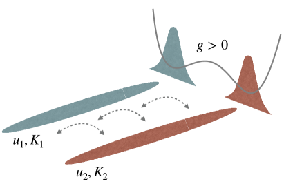
Figure 1: Schematic picture of the system studied in this paper. It consists of two unequal Luttinger liquids, with sound velocities $u_{i}$ and Luttinger parameters $K_{i}$ ($i=1,2$). We quench the system by switching off the tunnelling $g$, starting from a non zero value (both ground state and finite temperature thermal states are considered as initial states). This corresponds to suddenly raising the barrier of the double well potential separating the two sides.

In the theoretical description, it is often assumed that the two TLLs are identical, meaning they are characterized by equal sound velocities and Luttinger parameters. In this case, the theory consists of a quantum sine-Gordon model and a free boson Kardar_FermionicJosephsonJunctionAsSineGordon ; Gritsev_LinearResponseCoupledCondensates , describing respectively the antisymmetric and symmetric combinations of the phase fields (see section II for proper definitions). Importantly, as a consequence of the symmetry between the two TLLs, these two sectors are not coupled and thus can be treated as isolated systems. In particular, time-dependent correlation functions of the antisymmetric sector (directly related to interference measurements Polkovnikov_InterferenceCondensates ) after a sudden change in the tunnelling strength (a so-called quantum quench Calabrese_QuenchesCorrelationsPRL ) have been widely studied Imambekov_LectureNotesMatterInterferometry . They have been obtained by relying, for example, on a simple harmonic approximation Iucci_QuenchLL ; Iucci_QuenchSineGordon ; Foini_CoupledLLsMassiveMassless ; Foini_CoupledLLSchmiedtmayerMassive and, more recently, on a refined selfconsistent version of it vanNieuwkerk_QuenchSineGordonSelfConsistentHarmonicApprox ; vanNieuwkerk_TunnelCoupledBoseGasesLowEnergy . Exact results have been further obtained at the Luther–Emery point Iucci_QuenchSineGordon , by means of techniques such as integrability Bertini_QuenchSineGordon ; Cubero_QuenchAttractiveSineGordon ; Gritsev_LinearResponseCoupledCondensates and semi-classical methods Kormos_SemiclassicalQuantumSG ; Moca_SemiclassicalQuantumSG . A truncated conformal approach was considered in Kukuljan_QuenchSineGordonTruncatedConformalApproach ; Horvath_TruncatedApprox , while a combination of analytic (based on Keldysh formalism kamenev2011field ) and numerical methods was used in DallaTorre_QuenchSineGordonMasslessMassive . Finally, an effective model for the relative degrees of freedom was recently derived in Tononi_DynamicsTunnellingQuasicondensates . In these studies the existence of a prethermal regime was demonstrated.

Much less attention has been devoted so far to the effect of introducing an “imbalance” between the two systems. On the theory side such a case is interesting since, due to the presence of two velocities, one can expect multiple lightcones to emerge, separating different decaying regimes (as opposed to the single lightcone effect Calabrese_QuenchesCorrelationsPRL ; Cheneau_ExperimentalLightcones usually observed in systems of identical TLLs Foini_CoupledLLSchmiedtmayerMassive ; Langen_ThermalCorrelationsIsolatedSystems ). Because of the coupling between the modes one can also expect that the prethermal regime evidenced in the antisymmetric sector to decay into another final regime. Whether such a regime could be characterized by a single temperature despite the integrable nature of the underlying model Rigol_RelaxationHardCoreBosons ; Rigol_GGE is an interesting question. However due to the complexity of such a situation the asymmetric case has been much less studied. Noteworthy exceptions are provided by Ref. Langen_UnequalLL ; Kitagawa_DynamicsPrethermalizationQuantumNoise , where, relying on a phenomenological approach for the quench (especially concerning the initial state), the authors consider different forms of imbalance for two examples of systems described by LLs.

Given the importance of the physical effects in the asymmetric situation, it would thus be highly desirable: i) to have a full theoretical derivation of the quench of two different TLLs; ii) to allow for all possible sources of imbalance between them and disentangle the effects coming from unequal sound velocities $u_{i}$ from the ones related to different Luttinger parameters $K_{i}$ ($i=1,2$). Such a study is the goal of the present paper.

The paper is organized as follows. In section II we introduce the model and the quench dynamics we focus on. Section III and section IV discuss the Bogoliubov transformation which diagonalize the hamiltonian at initial time and introduce the correlation functions of interest, respectively. In section V a detailed analysis of the dynamics when starting from the ground state (i.e., at zero temperature) of the initial hamiltonian is carried out. The same analysis is extended to quenches starting from a thermal states in section VI. A discussion of the results, also in connection with previous literature, is left to section VII. Conclusions and future perspectives are finally collected in section VIII. Details regarding the calculations are reported in the appendices.

II Setting of the quench

We consider two different Luttinger liquids which are initially tunnel-coupled and then evolve independently: this is one of the simplest situation one can look at, since the evolution is the one of two free (compactified) bosons, while the coupling between the two is only in the initial state. This protocol has also the advantage to be easily implementable in a controlled way in cold atom experiments.

Microscopically, the system corresponds to two interacting 1d Bose gases, represented by bosonic fields $\Psi_{i}$ ($i=1,2$) of mass $M_{i}$ and short-ranged two-body interactions that can be represented by a delta function of strength $\mathcal{U}_{i}$. We are going to work with their phase $\theta_{i}(x)$ and the fluctuation of the densities $n_{i}(x)$, related to the original field via the bosonization formula Haldane_LuttingerLiquid ; Cazalilla_RevUltracold ; giamarchi2004

$$\Psi_{i}(x)=\sqrt{\rho_{i}+n_{i}(x)}e^{i\theta_{i}(x)}\ ,$$ (1)

with $[n_{i}(x),\theta_{j}(x^{\prime})]=i\hbar\delta(x-x^{\prime})\delta_{i,j}$ and $\rho_{i}$ is the average density of the $i$-th tube. In terms of these variables, the system is supposed to be prepared in the ground state (or in a thermal state) of the (generalized) Sine-Gordon Hamiltonian

$$H_{\text{initial}}^{\text{SG}}=H_{1}+H_{2}-\frac{g}{2\pi}\int{\rm d}x\ \cos(\theta_{1}(x)-\theta_{2}(x)),$$ (2)

where $H_{i}$ are the Luttinger liquid Hamiltonians giamarchi2004

$$H_{i}=\frac{\hbar}{2\pi}\int{\rm d}x\ \left[u_{i}K_{i}(\nabla\theta_{i})^{2}+\frac{u_{i}}{K_{i}}(\pi n_{i})^{2}\right]\ ,$$ (3)

and the cosine term originates from the tunnelling ($\Psi_{1}^{\dagger}\Psi_{2}+\text{h.c.}$), with strength tuned by $g$. In (3) $K_{i}$ is the Luttinger liquid parameter which encodes the interaction of the system and $u_{i}$ is the speed of sound. They are related to the microscopic parameters. Such relations are known analytically in the weak interaction regime

$$K_{i}=\hbar\pi\sqrt{\frac{\rho_{i}}{M_{i}\mathcal{U}_{i}}}\ ,\quad u_{i}=\sqrt{\frac{\mathcal{U}_{i}\rho_{i}}{M_{i}}}\ ,$$ (4)

and can be extracted numerically otherwise Cazalilla_RevUltracold . Therefore one can get unequal TLLs in many different settings, depending on the values of $M_{i},\mathcal{U}_{i}$ and $\rho_{i}$.

Hereafter we will set $\hbar=1$. At time $t=0$ the interaction between the two systems is switched off and the final Hamiltonian simply reads

$$H_{\text{final}}=H_{1}+H_{2}\ .$$ (5)

As the study of the initial hamiltonian (2) is particularly involved, we resort to a semiclassical (harmonic) approximation

$$H_{\text{initial}}^{\text{SC}}=H_{1}+H_{2}+\frac{g}{4\pi}\int{\rm d}x\ (\theta_{1}(x)-\theta_{2}(x))^{2}\ .$$ (6)

Note that in our quench the approximation is only in the initial state, while the dynamics can be obtained exactly. Such approximation is expected to hold as long as the cosine term in (2) is highly relevant in a renormalization group (RG) sense (in the case of identical TLLs, this corresponds to $K$ large enough giamarchi2004 , while the same RG analysis is missing for the more generic case considered here; note, however, that in the experiments involving bosons with contact interactions we can safely assume that we are in the relevant regime). Remarkably, for identical TLLs, it has been shown by means of exact calculations that the dynamics starting from (6) is qualitatively the same as from the Luther–Emery point where the full cosine term can be taken into account Iucci_QuenchSineGordon .

The fields $\theta_{i}$ and $n_{i}$ admit a decomposition in normal modes

$$\begin{array}[]{ll}\displaystyle\theta_{i}(x)=&\displaystyle\frac{i}{\sqrt{L}}\sum_{p\neq 0}\ e^{-ipx}\sqrt{\frac{\pi}{2K_{i}|p|}}(b^{{\dagger}}_{i,p}-b_{i,-p})\displaystyle+\frac{1}{\sqrt{L}}\theta_{i,0}\end{array}$$ (7)

$$\begin{array}[]{ll}\displaystyle n_{i}(x)=&\displaystyle\,\frac{1}{\sqrt{L}}\sum_{p\neq 0}e^{-ipx}\sqrt{\frac{|p|K_{i}}{2\pi}}(b^{{\dagger}}_{i,p}+b_{i,-p})\displaystyle+\frac{1}{\sqrt{L}}n_{i,0}\ .\end{array}$$ (8)

where $L$ is the system size. In the rest of the paper we will only focus on the thermodynamic limit (TDL), namely infinite system size. Finite-size effects will be discussed elsewhere. In terms of these bosons the final Hamiltonian is diagonal, namely

$$H_{\text{final}}=u_{1}\sum_{p\neq 0}|p|b^{{\dagger}}_{1,p}b_{1,p}+u_{2}\sum_{p\neq 0}|p|b^{{\dagger}}_{2,p}b_{2,p}\ ,$$ (9)

where the zero modes (i.e., $\theta_{i,0},n_{i,0}$) have been neglected. The Hamiltonian $H_{\text{initial}}^{\textrm{SC}}$, instead, is quadratic but needs to be diagonalized via a Bogoliubov transformation (see Section III below).

To highlight the difference with the case of two identical systems it is useful to introduce the symmetric ($+$) and antisymmetric ($-$) modes

$$\begin{array}[]{ll}\displaystyle\theta_{\pm}(x)=\frac{1}{\sqrt{2}}(\theta_{1}(x)\pm\theta_{2}(x))\\ \vspace{-0.2cm}\\ \displaystyle n_{\pm}(x)=\frac{1}{\sqrt{2}}(n_{1}(x)\pm n_{2}(x))\end{array}$$ (10)

which satisfy canonical commutation relations. In terms of these variables the final Hamiltonian reads

$$H_{\text{final}}=\displaystyle\frac{1}{2\pi}\int{\rm d}x\left\{uK\left[(\nabla\theta_{+})^{2}+(\nabla\theta_{-})^{2}\right]\right.\\ \left.\qquad\qquad+\frac{u}{K}\left[(\pi n_{+})^{2}+(\pi n_{-})^{2}\right]\right\}\\ +\frac{1}{\pi}\int{\rm d}x\left\{\Lambda_{\theta}\nabla\theta_{+}\nabla\theta_{-}+\Lambda_{n}\pi^{2}n_{+}n_{-}\right\}$$ (11)

with

$$\frac{u}{K}=\frac{1}{2}\left(\frac{u_{1}}{K_{1}}+\frac{u_{2}}{K_{2}}\right)\quad uK=\frac{1}{2}\left(u_{1}K_{1}+u_{2}K_{2}\right)$$ (12)

$$\Lambda_{\theta}=\frac{1}{2}\left(u_{1}K_{1}-u_{2}K_{2}\right)\quad\Lambda_{n}=\frac{1}{2}\left(\frac{u_{1}}{K_{1}}-\frac{u_{2}}{K_{2}}\right)\ .$$ (13)

Therefore we see that in the case of two identical systems the final hamiltonian dispay decoupling between symmetric and antisymmetric sectors and the quench occurs only in the antisymmetric one.

The situation that we consider in this work is more involved as this decoupling is not possible and to study correlation functions of $\theta_{-}$, which are usually those of experimental interest, one has to consider the dynamics of $\theta_{1}$ and $\theta_{2}$ which are correlated via the initial condition.

III Bogolioubov transformation for two species of bosons

In order to characterize the evolving state we aim at diagonalizing the initial Hamiltonian $H_{\text{initial}}^{\textrm{SC}}$ and write it as

$$H_{\text{initial}}^{\text{SC}}=\sum_{p\neq 0}\lambda_{m,p}\eta_{m,p}^{{\dagger}}\eta_{m,p}+\sum_{p\neq 0}\lambda_{0,p}\eta_{0,p}^{{\dagger}}\eta_{0,p}\ ,$$ (14)

up to an unimportant overall constant, which we neglect. The meaning of the subscripts $m,0$ will be clearer in the following: they emphasize that, as we are going to show, the two diagonal modes above are massive ($m$) and massless ($0$) respectively.

The transformation bringing the hamiltonian in the form (14) amounts to a Bogoliubov rotation of a four component vector, mixing the modes $(p,-p)$ of the two initial species of bosons. Specifically, we introduce the vectors of bosons of the initial and the final Hamiltonian, $\bm{\eta}^{{\dagger}}_{p}=(\eta_{m,p}^{{\dagger}}\,\eta_{m,-p}\,\eta_{0,p}^{{\dagger}}\,\eta_{0,-p})$ and $\bm{b}^{{\dagger}}_{p}=(b_{1,p}^{{\dagger}}\,b_{1,-p}\,b_{2,p}^{{\dagger}}\,b_{2,-p})$. These two are related by a matrix multiplication $\bm{b}_{p}=B(\hat{\varphi}_{p})\bm{\eta}_{p}$ with $B(\hat{\varphi}_{p})$ depending on the set of parameters $\hat{\varphi}_{p}=\{\varphi_{1,p},\varphi_{2,p},\Delta_{p},\phi_{p}\}$ and parametrized as follows Elmfors_Bogoliubov

$$B(\hat{\varphi}_{p})=\begin{bmatrix}B_{2}(\varphi_{1,p})\cos\phi_{p}&B_{2}(\varphi_{2,p}-\Delta_{p})\sin\phi_{p}\\ \vspace{-0.2cm}\\ -B_{2}(\varphi_{1,p}+\Delta_{p})\sin\phi_{p}&B_{2}(\varphi_{2,p})\cos\phi_{p}\end{bmatrix}$$ (15)

with

$$B_{2}(\varphi)=\left[\begin{matrix}\cosh\varphi&\sinh\varphi\\ \vspace{-0.2cm}\\ \sinh\varphi&\cosh\varphi\end{matrix}\right].$$ (16)

Details on the derivation are reported in Appendix A. The parameters of the matrix $B(\hat{\varphi}_{p})$ in (15) have the following interpretation: $\varphi_{1,p}$ and $\varphi_{2,p}$ define Bogoliubov rotations associated to the two bosons, separately. $\phi_{p}$ is the mixing angle between them. Finally, $\Delta_{p}$ exists only when the Bogoliubov rotation and the mixing of different bosons appear at the same time Elmfors_Bogoliubov . Explicitly, they are given by

$$\begin{array}[]{c}\displaystyle\varphi_{1,p}=\frac{1}{2}\log\left(\frac{\lambda_{m,p}}{u_{1}|p|}\right)\displaystyle\qquad\varphi_{2,p}=\frac{1}{2}\log\left(\frac{\lambda_{0,p}}{u_{2}|p|}\right)\displaystyle\qquad\Delta_{p}=\Delta=\frac{1}{2}\log\left(\frac{u_{1}}{u_{2}}\right)\end{array}$$

$$\phi_{p}=\text{arctan}\left[\frac{\sqrt{\epsilon_{1,p}^{2}-(u_{1}p)^{2}}\sqrt{\epsilon_{2,p}^{2}-(u_{2}p)^{2}}}{(\epsilon_{1,p}^{2}-\epsilon_{2,p}^{2})+\sqrt{(\epsilon_{1,p}^{2}+\epsilon_{2,p}^{2})^{2}-\left[(u_{2}p)^{2}\epsilon_{1,p}^{2}+(u_{1}p)^{2}\epsilon_{2,p}^{2}-(u_{1}p)^{2}(u_{2}p)^{2}\right]}}\right]\,$$ (18)

in terms of (for $i=1,2$)

$$\begin{array}[]{l}\displaystyle\epsilon_{i,p}=\sqrt{u_{i}|p|\left(u_{i}|p|+\frac{g}{2K_{i}|p|}\right)},\end{array}$$ (19)

and the eigenvalues of the hamiltonian (14) (for $k=m,0$)

$$\lambda_{k,p}=\frac{1}{\sqrt{2}}\sqrt{\epsilon_{1,p}^{2}+\epsilon_{2,p}^{2}\pm\sqrt{(\epsilon_{1,p}^{2}+\epsilon_{2,p}^{2})^{2}-4\left[(u_{2}p)^{2}\epsilon_{1,p}^{2}+(u_{1}p)^{2}\epsilon_{2,p}^{2}-(u_{1}p)^{2}(u_{2}p)^{2}\right]}}\ .$$ (20)

where the $+\,(-)$ sign is associated to the $m\,(0)$-mode. Note that, at the leading order in $p\to 0$, the eigenvalues (20) read

$$\lambda_{m,p}=m_{0}\ ,\qquad\qquad\lambda_{0,p}=a|p|\ ,$$ (21)

with

$$m_{0}=\sqrt{\frac{gu}{K}}\ ,\qquad\qquad a=\sqrt{\frac{u_{1}u_{2}}{K_{1}K_{2}}}K\,$$ (22)

in terms of the parameters in (12). Therefore, as anticipated, they describe a massive and a massless mode. Note also that, in the limit of equal TLLs, they would coincide with the antisymmetric and the symmetric modes, respectively.

IV Correlation functions after the quench

We will be mostly interested in the correlation functions of vertex operators

$$C_{\pm}(x,t,T_{0})\equiv\langle e^{i\sqrt{2}[\theta_{\pm}(x,t)-\theta_{\pm}(0,t)]}\rangle_{T_{0}}=\\ =e^{-\langle[\theta_{\pm}(x,t)-\theta_{\pm}(0,t)]^{2}\rangle_{T_{0}}}\ ,$$ (23)

where the expectation value $\langle\cdot\rangle_{T_{0}}$ is on the initial state, which we choose to be either the ground state ($T_{0}=0$) or a finite temperature ($T_{0}\neq 0$) equilibrium state of the initial hamiltonian ${H_{\text{initial}}^{\text{SC}}}$.

While the function $C_{-}(x,t,T_{0})$ is of clear experimental relevance and has been directly measured using matter-wave interferometry Kuhnert_ExpEmergenceCharacteristicLength1d ; Langen_ThermalCorrelationsIsolatedSystems ; Langen_ExperimentGGE ; Gring_Prethermalization , observables within the symmetric sector as $C_{+}(x,t,T_{0})$ have not been measured so far. Nonetheless, very recently, it was pointed out that that correlation functions in the symmetric sector also contribute to the measured density after time-of-flight vanNieuwkerk_ProjectivePhaseMeasurements , thus giving hopes for their future measurements.

Note that in our approach, due to the absence of decoupling between symmetric and antisymmetric variables, $\theta_{\pm}$ are not anymore the preferable variables to work with (as it was the case in the symmetric quench Foini_CoupledLLsMassiveMassless ; Foini_CoupledLLSchmiedtmayerMassive ). Instead, we will stick to the initial fields, $\theta_{1}$ and $\theta_{2}$. In terms of those variables, the one (two) point function of the symmetric or antisymmetric fields is recast into a two (four) point function.

We start by defining the parameters $\hat{\epsilon}_{p}=\{u_{1}|p|,u_{2}|p|\}$ entering in the definition of the time evolution operator

$$U(\hat{\epsilon}_{p},t)\equiv\begin{bmatrix}e^{-iu_{1}|p|t}&0&0&0\\ 0&e^{iu_{1}|p|t}&0&0\\ 0&0&e^{-iu_{2}|p|t}&0\\ 0&0&0&e^{iu_{2}|p|t}\end{bmatrix}$$ (24)

and the matrices

$$\begin{array}[]{ll}\displaystyle P^{\pm}\equiv&\displaystyle\sum_{ij}\frac{(\pm 1)^{i+j}}{4K_{i}K_{j}}\begin{bmatrix}\delta_{i1}\delta_{j1}&\delta_{i1}\delta_{j2}\\ \vspace{-0.2cm}\\ \delta_{i2}\delta_{j1}&\delta_{i2}\delta_{j2}\end{bmatrix}\otimes\begin{bmatrix}1&-1\\ \vspace{-0.2cm}\\ -1&1\end{bmatrix}\end{array}$$ (25)

where $\otimes$ denotes the Kronecker product.

For a generic quench starting from a thermal state of (6) at temperature $T_{0}$, Eq. (23) takes the compact form (see Appendix B for details)

$$\begin{array}[]{ll}\displaystyle C_{\pm}(x,t,T_{0})\displaystyle=\exp\left[-\int_{0}^{\infty}{\rm d}p\ e^{-\alpha^{2}p^{2}}\frac{2}{p}(1-\cos px)\right.\\ \vspace{-0.2cm}\\ \displaystyle\qquad\Big{(}W_{22}^{\pm}\text{cotanh}\left(\frac{\lambda_{m,p}}{2T_{0}}\right)\displaystyle\left.+W_{44}^{\pm}\text{cotanh}\left(\frac{\lambda_{0,p}}{2T_{0}}\right)\Big{)}\right]\ .\end{array}$$ (26)

For convenience we have introduced an ultraviolet cutoff $\alpha^{-1}$. We further denoted by $W^{\pm}_{\mu\nu}$ the elements of the matrices

$$W^{\pm}\equiv B^{\dagger}(\hat{\varphi}_{p})U^{\dagger}(\hat{\epsilon}_{p},t)P^{\pm}U(\hat{\epsilon}_{p},t)B(\hat{\varphi}_{p})\ .$$ (27)

Note that only two elements of the whole matrices are needed to fully characterize the correlation functions (26). Moreover, thanks to the quadratic approximation in the initial hamiltonian, they can be written explicitly (see Eq. (66) in Appendix B).

In order to define effective temperatures for $C_{\pm}$, we are going to compare these post-quench correlations with the equilibrium ones at finite temperature $T$

$$\begin{array}[]{l}\displaystyle C_{\pm}^{\text{eq}}(x,t,T)=\exp\left[-\int_{0}^{\infty}{\rm d}p\ e^{-\alpha^{2}p^{2}}(1-\cos px)\frac{1}{2p}\right.\\ \vspace{-0.2cm}\\ \displaystyle\qquad\left.\times\left[\frac{1}{K_{1}}\text{cotanh}\left(\frac{u_{1}|p|}{2T}\right)+\frac{1}{K_{2}}\text{cotanh}\left(\frac{u_{2}|p|}{2T}\right)\right]\right]\end{array}$$ (28)

which present an exponential decay in space with (inverse) correlation length

$$\xi_{T}^{-1}=\frac{\pi}{2}\left(\frac{1}{u_{1}K_{1}}+\frac{1}{u_{2}K_{2}}\right)T\ .$$ (29)

V Quench from the ground state

We consider here the quench from the ground state ($T_{0}=0$) of the Hamiltonian (6) and we defer the solution of the dynamics from a thermal state at temperature $T_{0}$ to section VI. In this section, expectation values over the ground state will be simply denoted as $\langle\cdot\rangle$.

V.1 Eigenmodes dynamics

An important observation is that in the limit $T_{0}\to 0$, we have $\text{cotanh}(\lambda_{k,p}/(2T_{0}))\to 1$ in Eq. (26), and it turns out that the leading order as $p\to 0$ of $C_{\pm}$ is captured uniquely by the first term, namely by the massive mode. The main contribution is better characterized by introducing the dynamics of the modes of phase and density. In particular, by using the following decomposition

$$\begin{array}[]{ll}\displaystyle\theta_{i}(x,t)=\sum_{p}e^{-ipx}\theta_{i}(p,t)\ ,\end{array}$$ (30)

one finds that

$$\begin{array}[]{ll}\displaystyle\theta_{i}(p,t)=\cos(u_{i}|p|t)\theta_{i}(p,0)-\alpha_{i,p}\sin(u_{i}|p|t)n_{i}(p,0)\end{array}$$ (31)

with $\alpha_{i,p}=\frac{\pi}{K_{i}|p|}$. The expectation value of the two point function over the ground state simplifies to

$$\langle\theta_{i}(p,t)\theta_{j}(-p,t)\rangle=\\ \cos(u_{i}|p|t)\cos(u_{j}|p|t)\langle\theta_{i}(p,0)\theta_{j}(-p,0)\rangle+\\ +\sin(u_{j}|p|t)\sin(u_{j}|p|t)\alpha_{ip}\alpha_{j-p}\langle n_{i}(p,0)n_{j}(-p,0)\rangle$$ (32)

for $i,j=1,2$, namely the initial correlations between $\theta_{i}$ and $n_{j}$ do not enter in the eigenmodes’ dynamics.

By plugging in the asymptotic expressions (21), one can further check that at the leading order in $p\to 0$ it holds

$$\langle\theta_{i}(p,0)\theta_{j}(-p,0)\rangle\simeq\frac{\pi}{4a|p|}\frac{u_{1}u_{2}}{K_{1}K_{2}}\frac{K}{u}$$ (33)

$$\langle n_{i}(p,0)n_{j}(-p,0)\rangle\simeq\frac{(-1)^{i+j}}{2\pi}\sqrt{\frac{K_{i}K_{j}m_{i}m_{j}}{u_{i}u_{j}}}\ ,$$ (34)

where we defined $m_{1}=m_{0}\cos\phi_{0}^{2}$, $m_{2}=m_{0}\sin\phi_{0}^{2}$ and $\phi_{p}\simeq\phi_{0}=\arctan\sqrt{\frac{K_{1}}{K_{2}}\frac{u_{2}}{u_{1}}}$. Note the initial anticorrelations between the densities of the two systems, which will have a role on the evolution of the phase.

To evaluate Eq. (26) at large scale and times, the strategy is to proceed order-by-order in powers of $p$, which successively lead to exponential and power-law decay of correlations. The leading divergence as $p\to 0$ in the integrand of $C_{\pm}(x,t)\equiv C_{\pm}(x,t,T_{0}=0)$ (cfr. Eq. (26)) comes from the initial density fluctuation while the part coming from the phase is negligible (this is due to the term $\alpha_{i,p}\alpha_{j,-p}\propto 1/p^{2}$ in the eigenmodes’ dynamics (32)). Notice that since the sound velocity $a$ appears only in the phase fluctuations, at this order the massless mode will not play any role in the correlation functions, consistently with what anticipated from Eq. (26).

If we define the building block of the correlations (26) as

$$c_{ij}(x,t)\equiv\langle(\theta_{i}(x,t)-\theta_{i}(0,t))(\theta_{j}(x,t)-\theta_{j}(0,t))\rangle$$ (35)

such that

$$\ln C_{\pm}=\frac{1}{2}\left(c_{11}+c_{22}\pm 2c_{12}\right),$$ (36)

then from (32) and (34) we have

$$c_{ij}(x,t)\simeq\frac{1}{2}\int_{0}^{\infty}{\rm d}p\ e^{-\alpha^{2}p^{2}}(1-\cos(px))\frac{(-1)^{i+j}}{p^{2}}\\ \times\sqrt{\frac{m_{i}m_{j}}{K_{i}K_{j}u_{i}u_{j}}}\Big{[}\cos((u_{i}-u_{j})pt)-\cos((u_{i}+u_{j})pt)\Big{]}\ .$$ (37)

If we neglect the cutoff, the integrals (37) can be analytically evaluated. They are of the form

$$\begin{array}[]{ll}\displaystyle\int_{0}^{\infty}{\rm d}p\ (1-\cos(px))\cos(upt)\frac{1}{p^{2}}\\ \vspace{-0.2cm}\\ \displaystyle\qquad\qquad=\begin{cases}\frac{\pi}{2}(-|tu|+|x|)&\ \text{if $|x|>|ut|$}\\ \vspace{-0.2cm}\\ 0&\text{if $|x|<|ut|$}\end{cases}\ .\end{array}$$ (38)

This shows explicitly the emergence of (sharp) light-cones, associated to each velocity $u$ within the correlation functions. Note that the light-cones are smoothened out (as physically expected) by reintroducing the cutoff.

Correlations like those in Eq. (37) appear in the exponent of $C_{\pm}$. Therefore, we expect the approximation (37) (whose integrand behaves as $1/p^{2}$) to capture only their exponential decay. A careful analysis should take into account possible power law corrections which come from the next-to-leading order correction (corresponding to an integrand $\propto 1/p$). These can be computed explicitly as follows

$$\int_{0}^{\infty}\frac{dp}{p}(1-\cos(px))\cos(upt)=\frac{1}{2}\ln\left|1-\frac{x^{2}}{u^{2}t^{2}}\right|$$ (39)

and therefore grow unbounded at large distances. As we are going to discuss, these terms are actually important, especially for the dynamics of $C_{+}$: in fact, there are regimes where the exponential behavior vanishes and power laws become leading.

V.2 Two-point function: transient, prethermal and stationary state

By looking at the Eq. (37), we can read the leading terms in the two point function (23), which presents a very rich behavior. Without loss of generality, we may assume $u_{1}>u_{2}$. Then, we find

$$\ln C_{\pm}(x,t)\simeq \displaystyle{-\frac{\pi}{16}\frac{m_{0}K}{u}\left[\frac{1}{K_{1}^{2}}2u_{1}t+\frac{1}{K_{2}^{2}}2u_{2}t\mp\frac{2}{K_{1}K_{2}}((u_{1}+u_{2})t-|u_{1}-u_{2}|t)\right]} x>2u_{1}t$$ (40a)

$$\ln C_{\pm}(x,t)\simeq \vspace{0.2cm}\displaystyle{-\frac{\pi}{16}\frac{m_{0}K}{u}\left[\frac{1}{K_{1}^{2}}x+\frac{1}{K_{2}^{2}}2u_{2}t\mp\frac{2}{K_{1}K_{2}}((u_{1}+u_{2})t-|u_{1}-u_{2}|t)\right]} 2u_{1}t>x>(u_{1}+u_{2})t$$ (40b)

$$\ln C_{\pm}(x,t)\simeq \vspace{0.2cm}\displaystyle{-\frac{\pi}{16}\frac{m_{0}K}{u}\left[\frac{1}{K_{1}^{2}}x+\frac{1}{K_{2}^{2}}2u_{2}t\mp\frac{2}{K_{1}K_{2}}(x-|u_{1}-u_{2}|t)\right]} (u_{1}+u_{2})t>x>2u_{2}t$$ (40c)

$$\ln C_{\pm}(x,t)\simeq \vspace{0.2cm}\displaystyle{-\frac{\pi}{16}\frac{m_{0}K}{u}\left[\frac{1}{K_{1}^{2}}+\frac{1}{K_{2}^{2}}\mp\frac{2}{K_{1}K_{2}}\right]x\mp\frac{\pi}{16}\frac{m_{0}K}{u}\frac{2}{K_{1}K_{2}}|u_{1}-u_{2}|t} 2u_{2}t>x>|u_{1}-u_{2}|t$$ (40d)

$$\ln C_{\pm}(x,t)\simeq \vspace{0.2cm}\displaystyle{-\frac{\pi}{16}\frac{m_{0}K}{u}\left[\frac{1}{K_{1}^{2}}+\frac{1}{K_{2}^{2}}\right]x} |u_{1}-u_{2}|t>x$$ (40e)

We stress that the expression above only captures the exponential decay of $C_{\pm}$, while power-law corrections are not included. In particular, within this approximation Eq. (40a) shows no spatial dependence: this does not mean that it does not decay at all, but that the next to leading term should be taken into account. By computing it, the corrected expression for $C_{+}$ in the large distance regime now reads

$$C_{+}^{\text{correct}}(x\gg 2u_{1}t,t)\propto{|x|^{-\frac{K}{a\,u}\frac{u_{1}u_{2}}{K_{1}K_{2}}}}\times\\ \times e^{-\frac{\pi}{16}\frac{m_{0}K}{u}\left[\frac{1}{K_{1}^{2}}2u_{1}t+\frac{1}{K_{2}^{2}}2u_{2}t-\frac{2}{K_{1}K_{2}}((u_{1}+u_{2})t-|u_{1}-u_{2}|t)\right]}\ .$$ (41)

This result is easy to understand from a physical point of view since before the quench $\theta_{-}$ is a massive mode, which does not decay to zero, while $\theta_{+}$ is massless with leading power-law correlations. In the regime of large distances and short times therefore we find the memory of such initial condition.

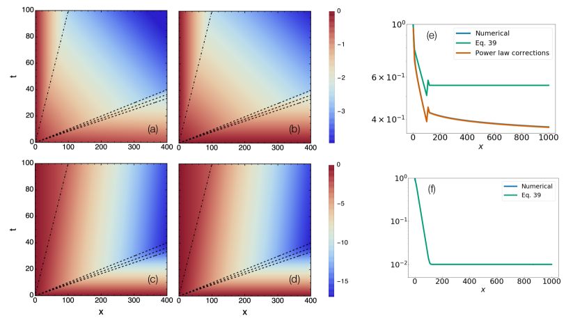
Figure 2: Logarithm of the correlation functions $C_{+}(x,t)$ (upper row: (a), (b), (e)) and $C_{-}(x,t)$ (lower row: (c), (d), (f)) after a quench from the ground state of the Hamiltonian (6) ($T_{0}=0$), as a function of distance $x$ and time $t$. The exact expressions from Eq. (26) (left panels: (a), (c)) are compared with the approximation in Eq. (40e) (central panels: (b), (d)). The parameters used are $u_{1}=6$, $u_{2}=5$, $K_{1}=20$, $K_{2}=10$, $g=40$ and $\alpha=1$. The position of the lightcones derived in Eq. (40e) are also shown. The dashed lines correspond to the lightcones at $x=2u_{1}t,(u_{1}+u_{2})t,2u_{2}t$ (in the chosen regime $u_{1}\approx u_{2}$ they are close to each other), separating the transient from the prethermal regime. The dot-dashed line corresponds to the last lightcone at $x=|u_{1}-u_{2}|t$, separating prethermal and final quasi-thermal regime. In the right panels (e),(f) we show a slice of the plots at time $t=10$ comparing the exact numerical results with Eq. (40e) (with an arbitrary amplitude) and for $C_{+}(x,t)$ the expression corrected by a power law decay in $x$ as in (41).

Moreover, from (40a) and its refined version (41), making use of the cluster property, $\lim_{x\to\infty}\langle O(x,t)O(0,t)\rangle=\langle O(t)\rangle^{2}$, we can read the behavior of the one point function

$$A_{\pm}(t)\equiv\langle e^{i\sqrt{2}\theta_{\pm}(0,t)}\rangle=e^{-\langle\theta_{\pm}^{2}(0,t)\rangle}\ .$$ (42)

For the antisymmetric sector we obtain the exponential decay

$$A_{-}(t)\simeq e^{-\frac{\pi}{16}\frac{m_{0}K}{u}\left[\frac{1}{K_{1}^{2}}u_{1}+\frac{1}{K_{2}^{2}}u_{2}+\frac{1}{K_{1}K_{2}}((u_{1}+u_{2})-|u_{1}-u_{2}|)\right]t}\ .$$ (43)

Note that for the symmetric quench ($K_{1}=K_{2}=K$ and $u_{1}=u_{2}=u$) we obtain the results of Calabrese_QuenchesCorrelationsPRL ; Calabrese_QuenchesCorrelationsLong ; Bistritzer_IntrinsingDephasingCoupledLL with the scaling dimension of $\theta_{-}$ equal to $h=1/(4K)$. Contrarily, for the symmetric sector, due to the power-law correction in (41), we find a vanishing one-point function at all times, i.e., $A_{+}(t)=0$.

From Eq. (40e) we see that $C_{\pm}$ reaches a stationary state at short length scales (large times). Note also that the next to leading order terms in $1/p$, such as integrals of the form (39) do not lead to important time corrections in the limit of large times and that formally one expects the limit of $t\to\infty$ to be really time independent as all the oscillating factors die out. From (40e), one can therefore read off an associated correlation length

$$\xi_{\text{Q}}^{-1}=\frac{\pi}{16}\frac{m_{0}K}{u}\left(\frac{1}{K_{1}^{2}}+\frac{1}{K_{2}^{2}}\right)\ ,$$ (44)

equal for both the symmetric and the antisymmetric mode, signaling that the correlations between the system one and two are lost. Comparing with (29) this defines an effective temperature

$$T^{\text{eff}}=\frac{m_{0}}{4}\left(\frac{K_{1}}{K_{2}}+\frac{K_{2}}{K_{1}}\right)\frac{u_{1}u_{2}}{4u^{2}}\ .$$ (45)

We dub this regime quasi-thermal, to emphasize that in spite of the integrable nature of the system, the final stationary state is well described in the large-scale limit by a unique correlation length, as in an equilibrium system. We will come back to the precise characterization of such state and on the meaning of the “temperature” later in the discussions. Then, if $u_{1}\approx u_{2}$, we have $u_{1}+u_{2}\approx 2u_{1}\approx 2u_{2}\gg|u_{1}-u_{2}|$, and from Eq. (40d), we see that one can define a quasi-stationary prethermal state with correlation length and thus effective temperature different for the symmetric and the antisymmetric mode

$$T^{\text{eff}}_{\pm}=\frac{m_{0}}{4}\left(\frac{K_{1}}{K_{2}}+\frac{K_{2}}{K_{1}}\mp 2\right)\frac{u_{1}u_{2}}{4u^{2}}\ .$$ (46)

This is the regime to which the system relaxes in the limit of $u_{1}=u_{2}$ and thus in particular for the symmetric quench. One can indeed check that for the symmetric quench ($u_{1}=u_{2}=u$ and $K_{1}=K_{2}=K$) we recover the results $T^{\text{eff}}_{-}={m_{0}}/{4}$ and $T^{\text{eff}}_{+}=0$ as expected from Calabrese_RevQuenches ; Foini_CoupledLLsMassiveMassless and from the decoupling of the modes.

In Fig. 2 we show the logarithm of the correlation functions $C_{\pm}(x,t)$ after a quench from the ground state of the Hamiltonian (6) ($T_{0}=0$) as a function of distance $x$ and time $t$. The exact expressions (left panels), numerically computed from Eq. (26), are compared with the small momenta approximation derived in Eq. (40e) (right panels). The position of the lightcones are also shown. While $C_{-}$ is well approximated by its exponential decay only in $x$ and $t$ (according to (40e)), for a correct description of $C_{+}$ power-law correction must be included, as is clearly visible by looking at a time slice in Fig. 2 (right panels). Note that for the parameters chosen, we are in the regime $u_{1}\approx u_{2}$. This is the reason why the regimes in (40b), (40c) and (40d), shown as dashed lines in the Figure, are not well separated. Finally, the dot-dashed line corresponds to the last lightcone at $x\approx|u_{1}-u_{2}|t$, separating prethermal and final quasi-thermal regime.

We then focus on the spatial decay of $C_{+}(x,t)$ and $C_{-}(x,t)$, for different (fixed) times. In Fig. 3 we compare this decay with the equilibrium correlation functions at temperatures $T^{\rm eff}$ and $T^{\rm eff}_{+}$ for $C_{+}(x,t)$ and $T^{\rm eff}$ and $T^{\rm eff}_{-}$ for $C_{-}(x,t)$, which capture the first two exponentially decaying regimes. In fact, for both correlations the longest time (short distance) shows the crossover between the fully stationary and the prethermal regime at distances around $|u_{1}-u_{2}|t$. After this decay $C_{+}(x,t)$ is characterized by a non monotonic behavior in the intermediate regimes. At large distances, differently as compared with $C_{-}(x,t)$, it does not saturate but it slowly decreases due to the power law corrections. The shortest times (long distance) of $C_{-}(x,t)$ instead show a light-cone like behavior toward a constant value for large distances. For the choice of parameters in the figure, the first three light cones in (40e) are not separately visible in $C_{-}(x,t)$ because they are very close (in $C_{+}(x,t)$ they correspond to the non monotonic behavior). The presence of the cut-off in (26) also tends to smear out the sharp transitions in (40e), as anticipated.

In Fig. 4 we compare the spatial decay of $C_{-}(x,t)$ and $C_{+}(x,t)$ in the quasi-thermal and in the prethermal regime, comparing also with the thermal correlations at temperature $T^{\rm eff}$, $T^{\rm eff}_{-}$ and $T^{\rm eff}_{+}$. The plot shows that the correlation length of the two quantities coincides in the first (quasi-thermal) regime and is also compatible with the equilibrium decay at temperature $T^{\rm eff}$. From this analysis therefore, the last regime can be thought (at the leading order) as a thermal regime, at least for the observables considered here. However, as we discuss in section V.3 the more robust thermodynamic interpretation of the stationary state is in terms of two temperatures, one for the first system and one for the second, which combined give rise coherently to Eq. (45). At larger distances the two correlations $C_{\pm}$ depart from the thermal regime and from each other, and agree with an equilibrium-like behavior at temperature $T^{\rm eff}_{-}$ and $T^{\rm eff}_{+}$, respectively (here we explicitly see a dependence on the observable chosen).

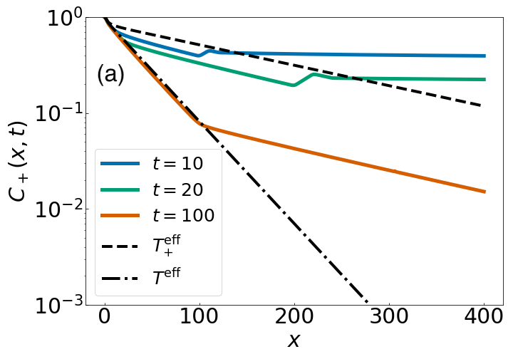
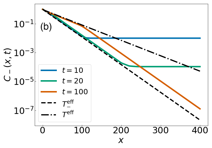
Figure 3: Space decay of $C_{+}(x,t)$ (panel (a)) and $C_{-}(x,t)$ (panel (b)) from (26) after a quench from the ground state of the Hamiltonian (6) ($T_{0}=0$), at different times $t=10,20,100$, compared with the equilibrium correlations at temperature $T^{\rm{eff}}$ and $T^{\rm eff}_{+}$ for $C_{+}(x,t)$ and $T^{\rm{eff}}$ and $T^{\rm eff}_{-}$ for $C_{-}(x,t)$. The parameters used are $u_{1}=6$, $u_{2}=5$, $K_{1}=20$, $K_{2}=10$, $g=40$ and $\alpha=1$.

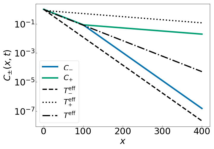
Figure 4: Space decay of $C_{-}(x,t)$ and $C_{+}(x,t)$ from (26) after a quench from the ground state of the Hamiltonian (6) ($T_{0}=0$), at time $t=100$, compared with the equilibrium correlations at temperature $T^{\rm{eff}}$, $T^{\rm eff}_{-}$ and $T^{\rm eff}_{+}$. The parameters used are $u_{1}=6$, $u_{2}=5$, $K_{1}=20$, $K_{2}=10$, $g=40$ and $\alpha=1$.

V.3 Interpretation as a two temperature system

The final Hamiltonian (5) has clearly two extensive and different conserved quantities: the energy of each subsystem. Therefore we expect to be able to define an effective temperature associated to each of them from the expectation values of the energy densities of the modes $\langle\epsilon_{i,p}\rangle\equiv u_{i}|p|\langle b_{i,p}^{{\dagger}}b_{i,p}\rangle$ with $i=1,2$ separately. In the limit of small momenta the expectation of each mode is dominated by a constant term equal for all the modes. Thanks to a classical equipartition approximation this allows us to interpret such constant as the effective temperature of the two systems Foini_CoupledLLSchmiedtmayerMassive . In particular we have

$$\begin{array}[]{l}\displaystyle\langle\epsilon_{1,p}\rangle\simeq\frac{m_{1}}{4}=\frac{m_{0}}{8}\frac{u_{1}}{K_{1}}\frac{K}{u}\equiv T_{1}^{\text{eff}},\\ \vspace{-0.2cm}\\ \displaystyle\langle\epsilon_{2,p}\rangle\simeq\frac{m_{2}}{4}=\frac{m_{0}}{8}\frac{u_{2}}{K_{2}}\frac{K}{u}\equiv T_{2}^{\text{eff}}.\end{array}$$ (47)

Note that

$$\langle\epsilon_{1,p}\rangle+\langle\epsilon_{2,p}\rangle=\frac{m_{0}}{4}\ ,$$ (48)

as for the symmetric quench Calabrese_RevQuenches ; Foini_CoupledLLsMassiveMassless . However, contrary to the symmetric limit where all the energy is stored in the antisymmetric sector (being isolated from the symmetric one), in the general case part of it is shared with the symmetric mode as well.

Note that if one supposes the two systems equilibrated at different temperatures, the correlation length associated to the decay of $C_{\pm}^{\text{eq}}$ turns out to be

$$\xi_{T_{1},T_{2}}^{-1}=\frac{\pi}{2}\left(\frac{T_{1}}{u_{1}K_{1}}+\frac{T_{2}}{u_{2}K_{2}}\right)\ ,$$ (49)

thus generalizing the expression (29). This is perfectly consistent with the effective temperatures (47) and the post quench correlation length (44). Specifically, the unique effective temperature, which we can read off from $C_{\pm}$ at large times, is related to the ones in (47) through

$$T^{\text{eff}}=\left(\frac{T_{1}^{\text{eff}}}{u_{1}K_{1}}+\frac{T_{2}^{\text{eff}}}{u_{2}K_{2}}\right)/\left(\frac{1}{u_{1}K_{1}}+\frac{1}{u_{2}K_{2}}\right)\ .$$ (50)

The two-temperature interpretation is further sustained by an FDT (fluctuation-dissipation theorem Callen_FDT ; Chou_ReviewFDT ; Cugliandolo_OutOfEquilibriumFDT ; Bouchaud_OutOfEquilibriumGlassySystems ) argument, analyzing the correlation and the response functions associated to the Green’s functions of the two systems – in the limit of small $\omega$ and small $p$ (see Appendix C). Note however that, while this interpretation is definitely more robust, it still is an approximation of the true underlying generalized Gibbs ensemble (GGE)Rigol_RelaxationHardCoreBosons ; Rigol_GGE . Moreover, this analysis requires more attention when trying to generalise to all observables (see the discussion section).

We close this section with an interesting remark. Knowing that in our quench (when $u_{1}\neq u_{2}$) the correlations between the two systems are lost in the stationary regime, one can expect the quasi-thermal state to which the system evolves to coincide with the final state reached by the same system of two bosons but after two independent quenches with initial energies (or initial masses, equivalenty) fixed by (47). As main difference, in this simpler quench, correlations are absent also in the initial state. If fact, since each $H_{i}$ ($i=1,2$) describes a conformally invariant system, one can directly apply the results of Calabrese_QuenchesCorrelationsPRL ; Calabrese_QuenchesCorrelationsLong for the correlation functions to see that at largest times

$$\langle e^{i\sqrt{2}(\theta_{\pm}(x,t)-\theta_{\pm}(0,t))}\rangle_{m_{1},m_{2}}=\\ =\langle e^{i(\theta_{1}(x,t)-\theta_{1}(0,t))}\rangle_{m_{1}}\langle e^{\pm i(\theta_{2}(x,t)-\theta_{2}(0,t))}\rangle_{m_{2}}\\ \simeq e^{-\frac{\pi}{2}\left(\frac{h_{1}m_{1}}{u_{1}}+\frac{h_{2}m_{2}}{u_{2}}\right)x}=e^{-\frac{\pi}{8}\left(\frac{m_{1}}{u_{1}K_{1}}+\frac{m_{2}}{u_{2}K_{2}}\right)x}\ .$$ (51)

The expectation value $\langle\cdot\rangle_{m_{1},m_{2}}$ in the first line is taken on a factorized state characterized by mass $m_{i}$ for the $i$-th system, which, therefore, simply splits in expectation values over the two systems (second line). The results of Calabrese_QuenchesCorrelationsPRL ; Calabrese_QuenchesCorrelationsLong have been applied to each $\langle\cdot\rangle_{m_{i}}$. In the last step, we used the explicit form $h_{i}=1/(4K_{i})$ for conformal dimensions of the (primary) operators $e^{\pm i\theta_{i}(x,t)}$ yellowbook . We stress, however, that, even if the result (51) is consistent with the last regime with associated effective temperature (50), the transient and prethermal regime are not captured by this simple picture.

VI Quench from a thermal state: corrections due to the initial temperature

If the initial state is prepared at finite temperature $T_{0}$, the full expression for the correlation function is still the one in Eq. (26). Now, however, one sees that, differently from the quench from the ground state, the leading contribution as $p\to 0$ includes a term coming from the massless mode. One can in principle carry a similar analysis as the one of the section V (notice in particular that Eq. (32) remains true also when starting from a thermal state), leading to different regimes during the evolution. In particular in Appendix D we sketch the derivation of the leading order term contributing to $C_{\pm}(x,t,T_{0})$ showing that the same light cones as for $T_{0}=0$ appear, with different correlation lengths and coherence times. Here however, we focus on the last two regimes (at large times), being the most relevant for the relaxation dynamics. As before, indeed, they allow for a definition of a prethermal and a quasi-thermal correlation length, for both the symmetric and the antisymmetric mode. The associated prethermal effective temperatures now read

$$\begin{array}[]{l}\displaystyle T^{\text{eff}}_{\pm}=\frac{m_{0}}{4}\left(\frac{K_{1}}{K_{2}}+\frac{K_{2}}{K_{1}}\mp 2\right)\frac{u_{1}u_{2}}{4u^{2}}\text{cotanh}\left(\frac{m_{0}}{2T_{0}}\right)\\ \vspace{-0.2cm}\\ \displaystyle\qquad+\Big{(}(1\pm 1)\frac{u_{1}u_{2}K_{1}K_{2}}{4u^{2}K^{2}}+\frac{1}{8}\frac{(u_{1}\pm u_{2})^{2}}{u^{2}}\Big{)}T_{0}\ .\end{array}$$ (52)

For the symmetric quench we recover $T^{\text{eff}}_{-}=\frac{m_{0}}{4}\text{cotanh}\left(\frac{m_{0}}{2T_{0}}\right)$ as in Sotiriadis_ThermalQuench and $T^{\text{eff}}_{+}=T_{0}$, as expected from the decoupling of the modes. A crucial observation here is that in this symmetric limit, the antisymmetric sector is almost unaffected by the true temperature of the system: in fact $T^{\text{eff}}_{-}\simeq{m_{0}}/{4}$, namely it is independent of $T_{0}$ (as long as it is low), while the thermal fluctuations are present only in the symmetric mode, as reflected by its effective temperature. The reason is that, while $\theta_{1}$ and $\theta_{2}$ are subject to thermal fluctuations, those cancel out in their difference (namely in $\theta_{-}$), while remaining present in their sum (i.e., in $\theta_{+}$) Langen_PrethermalizationNearIntegrable . Importantly, this picture completely changes as soon as an asymmetry is induced in the parameters $u_{i},K_{i}$ associated with the two tubes. In fact, Eq. (52) clearly shows a correction linear in $T_{0}$ for the effective temperature. To be more precise, for such linear correction to be present in the antisymmetric mode as well, different sound velocities, i.e., $u_{1}\neq u_{2}$, are needed (while a difference in the Luttinger parameters $K_{i}$ does not seem to play a main role here). In this case, the initial temperature plays a crucial role in the decay of all correlation functions. Specifically, since the term proportional to $T_{0}$ in (52) is always positive, it leads to a faster decay of $C_{\pm}$.

The final regime is instead described by

$$T^{\text{eff}}=\frac{m_{0}}{4}\left(\frac{K_{1}}{K_{2}}+\frac{K_{2}}{K_{1}}\right)\frac{u_{1}u_{2}}{4u^{2}}\text{cotanh}\left(\frac{m_{0}}{2T_{0}}\right)\\ \qquad+\Big{(}\frac{u_{1}u_{2}K_{1}K_{2}}{4u^{2}K^{2}}+\frac{1}{8}\frac{u_{1}^{2}+u_{2}^{2}}{u^{2}}\Big{)}T_{0}\ .$$ (53)

which also shows a term depending linearly on the initial temperature, leading to faster decaying correlations.

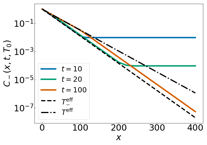
Figure 5: Space decay of $C_{-}(x,t,T_{0})$ from (26) with $T_{0}=0.5$, at different times $t=10,20,100$, compared with the equilibrium correlations at temperature $T^{\rm{eff}}$ and $T^{\rm eff}_{-}$. The parameters used are $u_{1}=6$, $u_{2}=5$, $K_{1}=20$, $K_{2}=10$, $g=40$ and $\alpha=1$.

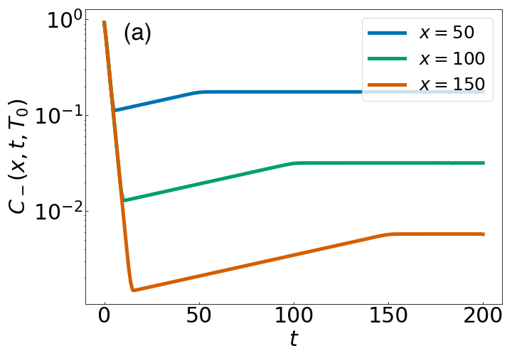
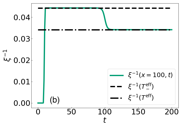
Figure 6: Panel (a): Time dependence of $C_{-}(x,t)$ from (26) with $T_{0}=0.5$, at different points in space $x=50,100,150$. Panel (b): Inverse correlation length (obtained as the spatial derivative of the exponent of Eq. (26)) at distance $x=100$ as a function of the time, compared with the equilibrium correlation length at temperature $T^{\rm{eff}}$ and $T^{\rm eff}_{-}$. The parameters used are $u_{1}=6$, $u_{2}=5$, $K_{1}=20$, $K_{2}=10$, $g=40$ and $\alpha=1$.

We mention that the limit of shallow quench $m_{0}\to 0$ (which amounts to doing nothing to the system) does not reproduce the equilibrium result $T^{\text{eff}}=T_{0}$. This signals that the limit of small momenta $p\to 0$ used in deriving $T^{\text{eff}}$ in (53) does not commute with the limit $m_{0}\to 0$.

In Fig. 5 we show how the effective temperatures derived above capture the main decay of the correlation functions, also in this quench starting from a thermal state. In particular, it shows the spatial decay of $C_{-}(x,t)$ starting from a thermal state at temperature $T_{0}=0.5$ and different times. The correlation lengths in the quasi-thermal and in the prethermal regime are compared with the one at equilibrium at temperature $T_{-}^{\rm eff}$ from (52) and $T^{\rm eff}$ from (53). The plateau attained at large distances (short times) is instead a property of the (massive) initial condition.

In Fig. 6 we plot the same correlator as a function of time. The top panel shows the time dependence of $C_{-}(x,t)$ again starting from a thermal state at temperature $T_{0}=0.5$ and different points in space. In the bottom panel, instead, the inverse correlation length at fixed distance is shown, as obtained from the spatial derivative of the exponent in Eq. (26). We see that in the regime $u_{1},u_{2}\gg|u_{1}-u_{2}|$ there is an intermediate prethermal regime where the correlation length is compatible with the equilibrium one at temperature $T^{\rm eff}_{-}$. At later times this quantity crosses over towards the asymptotic regime, compatible with the equilibrium one at temperature $T^{\rm eff}$.

VII Discussions

Let us make some comments about the results obtained in the previous sections, also in comparison with previous works.

To start with, since in our analysis we considered the generic case of different $u_{i}$ and $K_{i}$ (i=1,2), it is worth stressing the different role that these two parameters play in the dynamics. In fact, while we saw that, in the Hamiltonian (5), which governs the evolution after the quench, a coupling between symmetric and antisymmetric sector is present as soon as the systems one and two differ in either of the parameters (cfr. Eq. (11)), the consequences of having different $K_{i}$ or different $u_{i}$ separately are not the same. If $u_{1}=u_{2}$, then the correlation functions (40e) are much simplified and only one lightcone appears, with the dynamics never reaching the final regime (40e). This means that in this case symmetric and antisymmetric sectors show different effective final temperatures. Moreover the linear correction of the effective temperature of the antisymmetric sector (52) due to the initial temperature $T_{0}$ vanishes. Such observations further suggest that a sort of decoupling between different sectors still exists. In fact, in the final Hamiltonian (5), one could rescale the field $\theta_{i}$ by $\sqrt{K_{i}}$ and $n_{i}$ by $1/\sqrt{K_{i}}$ in such a way to respect canonical commutation relations and end up in a system of effectively identical TLLs, allowing for additional conservation laws than those associated to $H_{1}$ and $H_{2}$ (as for the symmetric quench). On the other hand having different $u_{i}$ but same $K_{i}$ does not modify the generic (richer) picture outlined in (40e), which is characterized by the presence of multiple lightcones and regimes. And, in fact, in this second case, the difference in the two tubes can not be reabsorbed in a rescaling of the variables similar to the one above. One peculiarity of this limit, however, is the fact that the effective temperature of the symmetric mode in the prethermal regime (46) is zero.

Let us now turn to the final stationary regime reached by the dynamics. As we discuss in section V.3 and Appendix C, such regime for many observables and in an RG sense (namely at large scales), is compatible with an equilibrium-like result associated to the two systems thermalized at temperatures $T_{1}^{\rm eff}$ and $T_{2}^{\rm eff}$, in accordance with the classical equipartition theorem and the FDT in its classical (low frequency) approximation. While this appears as a generalization to a two temperature equilibrium state of previous results Calabrese_QuenchesCorrelationsPRL ; Gring_Prethermalization ; Foini_CoupledLLsMassiveMassless , it might sound surprising given that the underlying dynamics conserves the energy of each mode. In fact, a GGE Rigol_RelaxationHardCoreBosons ; Rigol_GGE would rather appear from Eq. (26), if we would take into account the full dependence on the momenta $p$ in the integrals. However, as we have seen, the dynamics of the vertex operators of the antisymmetric mode (see the bottom panels of Figure 2) and the stationary part of the symmetric one (see the regime within the first lightcone at short distances in the top panels of Figure 2) are well captured by the leading order term in $p\to 0$ of the integrands which gives the expressions (40e) and in particular (40e). This fact by itself is quite remarkable since this is not usually the case for quenches in the LL (see Cazalilla_MasslessQuenchLL as main reference), where the underlying GGE describing the steady state is not thermal at all. Given a GGE of the form $\rho_{GGE}=\exp{(-\sum_{p}\beta(p)n(p))}$ (with $n(p)$ the conserved charges and $\beta(p)$ the associated temperatures, labelled by momentum $p$), this might or not be well approximated by a thermal ensemble, depending on the behaviour of the (inverse) temperatures $\beta(p)$ as a function of $p$. In particular, if we focus on the large scale limit, the modes that matter are the low energy ones and their behaviour is indeed what makes our quench in the tunnelling strength very different from the one in the interaction studied in Ref. Cazalilla_MasslessQuenchLL . Nonetheless, an example where the non-thermal behaviour clearly emerges also in our setup is given by the density-density correlations. In this case the leading term at large scale seems related to the first singularity in the small $p$ expansion (rather than a simple small $p$ expansion), giving rise to a power law decay. From the GGE point of view this means that the first term in the small $p$ expansion of $\beta(p)$ is not enough to capture the leading behavior. Physically, this contribution can be traced back to the presence of the massless mode, that now becomes leading. A complete analysis of this kind of correlations will be given elsewhere, from a different perspective Ruggiero_QuenchCoupledCFTs .

Moreover, in our discussion we referred to the regime (40d) (at least in the limit of $u_{1}\simeq u_{2}$) as a prethermal one, in analogy with the work Gring_Prethermalization (note however that, given the relaxation to a GGE discuss above, rather than a true thermalization, the term pre-relaxation, which already appeared in literature Fagotti_Prerelaxation_Free ; Bertini_Prerelaxation_Interacting , would be more appropriate). More generally, prethermalization has been discussed in many works and it is often associated to a slow evolving intermediate state attained by the system before a complete relaxation takes place, as it happens in integrable systems in presence of a small integrability breaking perturbation Bertini_LightconesIntegrabilityBreaking ; Bertini_PrethermalizationIntegrabilityBreaking ; Langen_PrethermalizationNearIntegrable ; Marcuzzi_PrethermalizationNonIntegrableSpinChain ; Kollar_PrethermalizationIntegrableSystems ; Mitra_IntegrabilityBreakingOutOfEquilibrium or in other more exotic scenarios as in Alba_NewPrethermalizationMechanism . In this sense, the fact of considering different $u_{i}$ can be seen as a symmetry breaking mechanism that removes the degeneracy of the hamiltonian driving the dynamics. In fact, from Figure 6 (particularly if focusing on the inverse correlation length, bottom panel) one clearly sees the presence of a first rapid transient regime, followed by a quasi-stationary one for a relatively large time (divergent in the limit $u_{1}\to u_{2}$) and later evolving towards its asymptotic value. Note however that in order for the final state to be reached, the prethermal plateau cannot be really time-independent and this is in fact clearly visible when looking at the correlation function $C_{-}$ itself (the top panel of the same Figure), which shows a slow ramp towards the final stationary regime. Note that this ramp can be increasing or decreasing according to the sign of $T_{-}^{\rm eff}-T^{\rm eff}$, which can be tuned upon varying $T_{0}$.

About the main experimental implications of our results, one of the most surprising effects of considering two TLLs with different parameters is the (positive) linear correction in $T_{0}$ to the effective temperature $T_{-}^{\rm eff}$ of the antisymmetric sector, in contrast to the insensitivity of the same in the symmetric scenario Gring_Prethermalization . This implies faster decaying correlations and it might be a non negligible effect in the dynamics, given the relative high temperature at which experiments are carried out. For example, we would expect a similar correction to take place in the experiment discussed in Pigneur_RelaxationPhaseLockedState : there, in principle, the very same analysis can be carried out, while for now a theoretical understanding of the observed “effective” dissipation mechanism is still missing vanNieuwkerk_QuenchSineGordonSelfConsistentHarmonicApprox ; vanNieuwkerk_TunnelCoupledBoseGasesLowEnergy ; Pigneur_EffectiveDissipativeModel (see also Polo_Josephson_damping_head-to-tail where the same problem is studied but within a different geometrical setup).

Remarkably, the phenomenological description of the unbalanced splitting protocol of Ref. Langen_UnequalLL for two bosonic tubes at different densities agrees in many aspects with the overall picture emerging from our general analysis of the quench dynamics in unbalanced TLLs coupled by tunnelling. There, in particular, the transition from a prethermal to a thermal regime, both characterized by an exponential decay of correlation functions, with a multi light-cone dynamics signalling the sharp transition between different correlation lengths was found, as well as an additive correction proportional to the initial true temperature $T_{0}$ to the final effective temperature, shared by both the symmetric and the antisymmetric sector. Such effects are indeed a consequence of the form of the initial correlations (fixed by phenomenological reasoning in Ref. Langen_UnequalLL , while derived in our case), whose leading term behaves as $p^{-2}$ (see Eqs. (71) and (72)). Moreover, the relation $T^{\text{eff}}=(T^{\text{eff}}_{-}+T^{\text{eff}}_{+})/2$ in Langen_UnequalLL , connecting the prethermal and the thermal effective temperatures, is found to hold in our more general setting (cfr. Eqs. (52) and (53)).

There are however some interesting differences. In particular the case of density imbalance, $\rho_{1}\neq\rho_{2}$, studied in Ref. Langen_UnequalLL , leads to the vanishing of the $n_{\pm}$ mixing term in (11) (i.e., $\Lambda_{n}=0$ in (13)), while more general imbalances (coming, for example, from different 1d interactions $U_{i}$) would allow for the presence of such a term. Moreover, due to the difference in the two protocols (namely, the starting point of Langen_UnequalLL is an imbalanced splitting of a single tube, while we start directly from two different tubes with non-zero tunnelling), our temperatures show a different dependence on the density as one can easily check by substituting the parameters (4) in our expressions. In particular, note that, in our protocol, if the imbalance is just in the densities and in the limit $T_{0}\to 0$, we get that the temperatures of the two systems given in (47) are the same, i.e., $T_{1}^{\text{eff}}=T_{2}^{\text{eff}}$, and therefore they also coincide with the final temperature of the symmetric and antisymmetric sectors. This, however, is not the case anymore at finite temperature $T_{0}\neq 0$, and a linear correction in $T_{0}$ appears also to the prethermal temperature $T^{\text{eff}}_{-}$ of the asymmetric sector, due to the difference between the two velocities.

Some of the effects mentioned above were also analyzed in Ref. Kitagawa_DynamicsPrethermalizationQuantumNoise , which was considering a two “spin” mixture, analagous to our two leg ladder system, and thus discuss a quench for a similar Hamiltonian. However in their case the initial state is chosen to be a factorized state of the symmetric and antisymmetric parts. For our quench this is not the case and the initial state does not simply factorize, thus leading to different time evolutions.

It would be very interesting to test the previously highlighted features, displaying strong differences as compared to the equal TLLs scenario. This could be done e.g. in experiments similar to the ones of the Vienna’s group Kuhnert_ExpEmergenceCharacteristicLength1d ; Langen_ThermalCorrelationsIsolatedSystems ; Langen_ExperimentGGE ; Gring_Prethermalization . Given the importance played by the sound velocities in the dynamics, the presence of the harmonic confinement potential (where the gas is trapped) leading to a spatially dependent velocity is clearly a highly unwanted complication. Fortunately, however, the recent realization of boxlike potentials in such experiments Jorg_privatecommunication shows great promise that the features analyzed in the present paper could be tested in a near future. Note that although here we mainly focused on vertex correlators, our analysis gives a full diagonalization of the problem, so in principle other correlation functions are also easily accessible.

VIII Conclusions

In this work we have studied a quench in the tunnelling strength of two TLLs with different parameters, under a quadratic approximation for the initial tunnel coupling term.

Our results show that the fact of considering two unqual systems leads to a much richer physics than the one observed in the symmetric scenario. This is manifested, for instance, in the emergence of multiple light cones. Moreover, under this dynamics, the prethermal regime discussed in Gring_Prethermalization is followed by a final stationary state, that we dubbed quasi-thermal, where symmetric and antisymmetric sectors display the same effective temperature (spatial decay). Due to the coupling between the symmetric/antisymmetric sectors, one observes also an important effect of the initial temperature on the correlation length (effective temperature) measured via the decay of the antisymmetric mode, which otherwise would be only slightly modified in the limit of large initial masses.

Our prediction could be tested in experiments similar to the ones performed Kuhnert_ExpEmergenceCharacteristicLength1d ; Langen_ThermalCorrelationsIsolatedSystems ; Langen_ExperimentGGE ; Gring_Prethermalization for the symmetric quenches.

Beyond the current work the generalized Bogolioubov transformations developed in this paper allow us to address also different settings and a natural sequel of this work would be to consider the opposite quench, namely from a massless (uncoupled) initial condition to a massive (coupled) dynamics Ruggiero_MasslessMassiveAsymmLLs . Another interesting direction to pursue is to understand the solution of the dynamics outlined in this work from the perspectives of a conformal field theory (CFT) approach Ruggiero_QuenchCoupledCFTs , generalizing the ideas of Calabrese_QuenchesCorrelationsPRL ; Calabrese_QuenchesCorrelationsLong ; Calabrese_RevQuenches to the quench of two independent CFTs coupled by a (conformal) initial condition.

Appendix A Bogoliubov transformation

We want to diagonalize the hamiltonian (6). To this aim, we go to Fourier space, where it can be decomposed as

$$H_{\text{initial}}^{\text{SC}}=\sum_{p\neq 0}\bm{b}^{{\dagger}}_{p}H_{p}\bm{b}_{p},$$ (54)

with $\bm{b}^{{\dagger}}_{p}=(b_{1,p}^{{\dagger}}\,b_{1,-p}\,b_{2,p}^{{\dagger}}\,b_{2,-p})$. Above, $H_{p}$ is of the form

$$\begin{bmatrix}w_{1,p}+D_{1,p}&-D_{1,p}&-C_{p}&C_{p}\\ -D_{1,p}&w_{1,p}+D_{1,p}&C_{p}&-C_{p}\\ -C_{p}&C_{p}&w_{2,p}+D_{2,p}&-D_{2,p}\\ C_{p}&-C_{p}&-D_{2,p}&w_{2,p}+D_{2,p}\end{bmatrix}$$

and ($i=1,2$)

$$w_{i,p}=\frac{u_{i}|p|}{2},\quad D_{i,p}=\frac{g}{8}\frac{1}{K_{i}|p|},\quad C_{p}=\sqrt{D_{1,p}D_{2,p}}\ .$$ (55)

The problem is thus reduced to the diagonalization of the $4\times 4$ matrix $H_{p}$. This can be achieved via a Bogoliubov transformation Bogoliubov_Bogoliubov ; Valatin_Bogoliubov , which is a linear transformation $B$ on the bosons $\bm{b}_{p}$. Restricting to real transformations, it has $16$ free parameters. However, it has to satisfy some constraints Elmfors_Bogoliubov . First of all, the $4$ bosonic modes defining $\bm{b}_{p}$ are not independent, but are instead related (in pairs) by $p\to-p$. This reduces the free parameters to 8, and constrains the corresponding Bogoliubov matrix to be of the form

$$B\equiv\begin{pmatrix}\alpha&\beta\\ \gamma&\delta\end{pmatrix},\quad\alpha=\begin{pmatrix}\alpha_{1}&\alpha_{2}\\ \alpha_{2}&\alpha_{1}\end{pmatrix}$$ (56)

and the same for $\beta,\gamma,\delta$. Moreover, we want $B$ to preserve canonical commutation relations, i.e.,

$$[\bm{b}_{p,\mu},\bm{b}_{p,\nu}^{\dagger}]=J_{\mu\nu},\quad J\equiv\begin{bmatrix}1\\ &-1\\ &&1\\ &&&-1\end{bmatrix}$$ (57)

where $\mu,\nu=\{1,2,3,4\}$. This requirement leads to the condition

$$BJB^{\text{t}}{=}J\ ,$$ (58)

namely $B$ must be a symplectic matrix. Eq. (58) is equivalent to

$$(\alpha_{1}^{2}-\alpha_{2}^{2})+(\beta_{1}^{2}-\beta_{2}^{2})=1$$

$$(\gamma_{1}^{2}-\gamma_{2}^{2})+(\delta_{1}^{2}-\delta_{2}^{2})=1$$

$$\alpha_{1}\gamma_{1}-\alpha_{2}\gamma_{2}+\beta_{1}\delta_{1}-\beta_{2}\delta_{2}=0$$

$$\alpha_{1}\gamma_{2}-\alpha_{2}\gamma_{1}+\beta_{1}\delta_{2}-\beta_{2}\delta_{1}=0.$$

If we take $(\alpha_{1}^{2}-\alpha_{2}^{2})\geq 0$ and the same for $\beta,\gamma,\delta$, the solutions can be parametrized by a Bogoliubov matrix of the form given in Eq. (15), with $B\equiv B(\hat{\varphi}_{p})$ depending on a set of $4$ parameters $\hat{\varphi}_{p}=\{\varphi_{1,p},\varphi_{2,p},\Delta_{p},\phi_{p}\}$. Finally, their value is uniquely fixed by the requirement for $B$ to diagonalize $H_{p}$. Note that this is not a standard diagonalization problem, because of the symplectic nature of $B$. The standard procedure Tsallis_Bogoliubov ; vanHemmen_Bogoliubov amounts to finding the spectrum of $H_{p}$, by introducing the matrix $H_{p}J$. This one can now be diagonalized in a standard way, meaning via a unitary transformation $T$ as

$$T^{-1}(H_{p}J)T=\Lambda_{p}J\ ,$$

with $\Lambda_{p}$ diagonal (the corresponding spectrum in our case is given by Eq. (20) in the main text). Eventually, one imposes $B^{\text{t}}H_{p}B=\Lambda_{p}$. This fixes the parameters $\hat{\varphi}_{p}$ to be of the form given in Eq. (18).

Appendix B Derivation of $C_{\pm}(x,t,T_{0})$, Eq. (26)

We start by considering the logarithm of $C_{\pm}(x,t,T_{0})$ defined in (23), i.e.,

$$\langle[\theta_{\pm}(x,t)-\theta_{\pm}(0,t)]^{2}\rangle_{T_{0}}.$$ (59)

If we expand the square inside the expectation value, it is the sum of 4 terms of the form

$$\langle\theta_{\pm}(x,t)\theta_{\pm}(y,t)\rangle_{T_{0}}=\frac{1}{2}\sum_{i,j=1,2}(\pm 1)^{i+j}\langle\theta_{i}(x,t)\theta_{j}(y,t)\rangle_{T_{0}}.$$ (60)

The problem is thus reduced to the evaluation of correlation functions of $\theta_{i}(x,t)$ ($i=1,2$). This can be achieved, as in section V.1, by looking at the the dynamics of $\theta_{i}(p,t)$. An alternative way, however, it to use the expansion of the fields $\theta_{i}(x,t)$ in terms of the creation/annihilation operators $b_{p,i}(t)$ (at $t=0$ it is given by Eq. (7) in the main text, with $b_{i,p}\equiv b_{i,p}(0)$), which evolve freely under the evolution operator $U(\hat{\epsilon}_{p},t)$, as defined in (24). Still, expectation values are to be taken on a thermal state of the hamiltonian (14), which is diagonal in the operators $\eta_{i,p}$ (cfr. Eq. (14)). Initial and final bosonic operators are related by the following sequence of transformations

$$\bm{b}_{p}(t)\quad\stackrel{{\scriptstyle U(\hat{\epsilon}_{p},t)}}{{\longrightarrow}}\quad\bm{b}_{p}(0)\quad\stackrel{{\scriptstyle B(\hat{\varphi}_{p})}}{{\longrightarrow}}\quad\bm{\eta}_{p}(0)\ ,$$ (61)

equivalent to

$$\bm{b}_{p}(t)=U_{p}(t)B(\hat{\varphi}_{p})\bm{\eta}_{p}(0)\ .$$ (62)

These considerations allow us to write

$$\langle\theta_{i}(x,t)\theta_{j}(y,t)\rangle=\sum_{p,q\neq 0}e^{-i(px-qy)}W^{\pm}_{\mu\nu}\langle\bm{\eta}_{p,\mu}^{\dagger}(0)\bm{\eta}_{q,\nu}(0)\rangle,$$ (63)

where the sum over the dumb indices $\mu,\nu=\{1,2,3,4\}$ is understood and the matrices $W^{\pm}$ have been defined in Eq. (27). Next, we observe that

$$\langle\bm{\eta}_{p,\mu}^{\dagger}(0)\bm{\eta}_{q,\nu}(0)\rangle=\delta_{p,q}\left(F^{\beta}(p)_{\mu\nu}+(\delta_{\mu 2}\delta_{\nu 2}+\delta_{\mu 4}\delta_{\nu 4})\right)\ ,$$ (64)

where we further defined the matrix

$$F^{\beta}(p)=\text{diag}(f_{m}^{\beta},f_{m}^{\beta},f_{0}^{\beta},f_{0}^{\beta})$$ (65)

and $f_{k}^{\beta}\equiv f_{k}^{\beta}(p)=\frac{1}{e^{\beta\lambda_{k,p}}-1}$ ($k=m,0$) is the Bose function (and $\lambda_{k,p}$ in Eq. (20)). Finally, by using (64) in Eq. (63), and (60) in Eq. (59), the exact expression of $C_{\pm}$ in Eq. (26) is easily obtained. The two matrix elements of $W^{\pm}$ explicitly appearing in the final expression, can be evaluated directly from (27) and, in terms of the parameters $\hat{\varphi}_{p}$ defining the Bogoliubov transformation, they read

$$\begin{array}[]{ll}\displaystyle W_{22}^{\pm}=&\displaystyle\Big{\{}\frac{\cos^{2}\phi_{p}}{4K_{1}}(\cosh(2\varphi_{1,p})-\cos(2u_{1}|p|t)\sinh(2\varphi_{1,p}))+\frac{\sin^{2}\phi_{p}}{4K_{2}}(\cosh(2(\Delta+\varphi_{1,p}))-\cos(2u_{2}|p|t)\sinh(2(\Delta+\varphi_{1,p})))\\ \vspace{-0.2cm}\\ &\displaystyle\pm\frac{\sin 2\phi_{p}}{4\sqrt{K_{1}K_{2}}}(-\cos((u_{1}-u_{2})|p|t)\cosh(\Delta+2\varphi_{1,p})+\cos((u_{1}+u_{2})|p|t)\sinh(\Delta+2\varphi_{1,p}))\Big{\}}\ ,\end{array}$$

$$\begin{array}[]{ll}\displaystyle W_{44}^{\pm}=&\displaystyle\Big{\{}\frac{\cos^{2}\phi_{p}}{4K_{2}}(\cosh(2\varphi_{2,p})-\cos(2u_{2}|p|t)\sinh(2\varphi_{2,p}))+\frac{\sin^{2}\phi_{p}}{4K_{1}}(\cosh(2(\varphi_{2,p}-\Delta))-\cos(2u_{2}|p|t)\sinh(2(\varphi_{2,p}-\Delta)))\\ \vspace{-0.2cm}\\ &\displaystyle\pm\frac{\sin 2\phi_{p}}{4\sqrt{K_{1}K_{2}}}(\cos((u_{1}-u_{2})|p|t)\cosh(2\varphi_{2,p}-\Delta)-\cos((u_{1}+u_{2})|p|t)\sinh(2\varphi_{2,p}-\Delta))\Big{\}}\ .\end{array}$$ (66)

Appendix C Two-time correlations and FDT in the stationary state

Here we study different Green’s functions of system one and two after a thermal quench and we discuss their relation. In particular the Keldysh, the retarded and the advanced Green’s functions of system $i=1,2$ are defined, respectively, as follows

$$\begin{array}[]{l}G_{i}^{K}(p,t_{2},t_{1})=\langle\{b_{i,p}(t_{1}),b_{i,p}^{{\dagger}}(t_{2})\}\rangle_{T_{0}}\ ,\\ \vspace{-0.2cm}\\ G_{i}^{R}(p,t_{2},t_{1})=\theta(t_{1}-t_{2})\langle[b_{i,p}(t_{1}),b_{i,p}^{{\dagger}}(t_{2})]\rangle_{T_{0}}\ ,\\ \vspace{-0.2cm}\\ G_{i}^{A}(p,t_{2},t_{1})=-\theta(t_{2}-t_{1})\langle[b_{i,p}(t_{1}),b_{i,p}^{{\dagger}}(t_{2})]\rangle_{T_{0}}\ ,\end{array}$$ (67)

where for completeness we consider the expectation value over a thermal state. These functions turn out to be time translational invariant and depend only on the difference $t=t_{1}-t_{2}$, immediately after the quench. Moreover the response function (retarded correlator) does not depend on the initial condition. In particular, at the leading order in $p\to 0$ they read

$$\begin{array}[]{l}\displaystyle G_{1}^{K}(p,t)\simeq\frac{1}{2u_{1}|p|}e^{-iu_{1}|p|t}\left[m_{1}^{T_{0}}+\left(\frac{u_{2}}{K_{2}}\frac{K}{u}+\frac{K_{1}u_{1}}{uK}\right)T_{0}\right]\\ \vspace{-0.2cm}\\ \displaystyle G_{2}^{K}(p,t)\simeq\frac{1}{2u_{2}|p|}e^{-iu_{2}|p|t}\left[m_{2}^{T_{0}}+\left(\frac{u_{1}}{K_{1}}\frac{K}{u}+\frac{K_{2}u_{2}}{uK}\right)T_{0}\right]\\ \vspace{-0.2cm}\\ \displaystyle G_{i}^{R\backslash A}(p,t)=\pm\theta(\pm t)\ e^{-iu_{i}|p|t}\quad\text{for $i=1,2$}\end{array}$$ (68)

with $m_{i}^{T_{0}}=m_{i}\ \text{cotanh}(m_{0}/2T_{0})$. Fourier transforming such functions in the frequency domain, one obtains

$$G_{i}^{K}(p,\omega)=\frac{2T^{T_{0},\rm eff}_{i}}{\omega}\ (G_{i}^{R}(p,\omega)-G_{i}^{A}(p,\omega))\ ,$$ (69)

with effective temperatures

$$\begin{array}[]{l}\displaystyle T_{1}^{T_{0},\text{eff}}=\frac{m_{1}^{T_{0}}}{4}+\left(\frac{u_{2}}{K_{2}}\frac{K}{u}+\frac{u_{1}K_{1}}{uK}\right)\frac{T_{0}}{4}\simeq\langle\epsilon_{1,p}\rangle_{T_{0}}\\ \vspace{-0.2cm}\\ \displaystyle T_{2}^{T_{0},\text{eff}}=\frac{m_{2}^{T_{0}}}{4}+\left(\frac{u_{1}}{K_{1}}\frac{K}{u}+\frac{u_{2}K_{2}}{uK}\right)\frac{T_{0}}{4}\simeq\langle\epsilon_{2,p}\rangle_{T_{0}}\ ,\end{array}$$ (70)

which are the generalization of (47) to finite temperature quenches. Eq. (69) is the celebrated fluctuation-dissipation theorem (FDT) in the limit of small frequencies (or classical limit) kamenev2011field , which states a fundamental relation between correlation and response functions in equilibrium systems.

Appendix D Leading analytic expressions of $C_{\pm}(x,t,T_{0})$ after a thermal quench

In this section we provide a derivation of the equations that give the leading order of the correlation functions $C_{\pm}(x,t,T_{0})$ and the effective temperatures (52) and (53) after a thermal quench.

As we mentioned in the main text, Eq. (32) still holds, also at finite temperature. The expectation values of the phase and density fluctuations at time $t=0$ however are modified, in particular by the massless mode. These read

$$\langle\theta_{i}(p,0)\theta_{j}(-p,0)\rangle\simeq\frac{\pi}{2a^{2}p^{2}}\frac{u_{1}u_{2}}{K_{1}K_{2}}\frac{K}{u}T_{0}=\frac{1}{p^{2}}\frac{\pi}{2uK}T_{0}$$ (71)

$$\begin{array}[]{c}\displaystyle\langle n_{i}(p,0)n_{j}(-p,0)\rangle\displaystyle\simeq\frac{1}{2\pi}\sqrt{\frac{K_{i}K_{j}}{u_{i}u_{j}}}\left[(-1)^{i+j}\sqrt{m_{i}^{T_{0}}m_{j}^{T_{0}}}\right.\\ \vspace{-0.2cm}\hfil\\ \displaystyle\left.+\sqrt{\frac{u_{k_{1}\neq i}u_{k_{2}\neq j}}{K_{k_{1}\neq i}K_{k_{2}\neq j}}}\frac{K}{u}T_{0}\right]\ ,\end{array}$$ (72)

with $m_{i}^{T_{0}}=m_{i}\text{cotanh}\left(\frac{m_{0}}{2T_{0}}\right)$ and $k_{1},k_{2}=1,2$. Therefore, in a thermal quench, both phase and density fluctuations contribute. The building blocks (35) become

$$\begin{array}[]{ll}\displaystyle c_{ij}(x,t)\simeq\frac{1}{2}\int_{0}^{\infty}{\rm d}p\ e^{-\alpha^{2}p^{2}}(1-\cos(px))\frac{1}{p^{2}}\displaystyle\Big{\{}\Big{[}(-1)^{i+j}\sqrt{\frac{m_{i}^{T_{0}}m_{j}^{T_{0}}}{K_{i}K_{j}u_{i}u_{j}}}+\frac{T_{0}}{uK}\left(\frac{K^{2}}{K_{1}K_{2}}\sqrt{\frac{u_{k_{1}\neq i}u_{k_{2}\neq j}}{u_{i}u_{j}}}+1\right)\Big{]}\cos((u_{i}-u_{j})pt)-\\ \vspace{-0.2cm}\\ \displaystyle\qquad\qquad\qquad\Big{[}(-1)^{i+j}\sqrt{\frac{m_{i}^{T_{0}}m_{j}^{T_{0}}}{K_{i}K_{j}u_{i}u_{j}}}+\frac{T_{0}}{uK}\left(\frac{K^{2}}{K_{1}K_{2}}\sqrt{\frac{u_{k_{1}\neq i}u_{k_{2}\neq j}}{u_{i}u_{j}}}-1\right)\Big{]}\cos((u_{i}+u_{j})pt)\Big{\}}\ .\end{array}$$ (73)

Note that this structure gives rise to the same light cones as for the quench from $T_{0}=0$. From this we can read the final correlation length (in the case $u_{1}\neq u_{2}$)

$$(\xi^{T_{0}}_{Q})^{-1}=\frac{\pi}{8}\Big{[}\frac{m_{0}}{2}\frac{K}{u}\left(\frac{1}{K_{1}^{2}}+\frac{1}{K_{2}^{2}}\right)\text{cotanh}\left(\frac{m_{0}}{2T_{0}}\right)+\frac{T_{0}}{uK}\left(\frac{K^{2}}{K_{1}K_{2}}\frac{u_{1}^{2}+u_{2}^{2}}{u_{1}u_{2}}+2\right)\Big{]}\ ,$$ (74)

which is compatible with the temperature (53). Note that this expression has a simple interpretation in terms of a two temperature system with temperatures given in (70), and generalizing Eqs. (47) to a thermal quench.

In addition, the prethermal correlation length of the symmetric and the antisymmetric mode (which can be deduced setting $u_{1}=u_{2}$ in the limit of large times) reads

$$(\xi^{T_{0}}_{\pm})^{-1}=\frac{\pi}{8}\Big{[}\frac{m_{0}}{2}\frac{K}{u}\left(\frac{1}{K_{1}^{2}}+\frac{1}{K_{2}^{2}}\mp\frac{2}{K_{1}K_{2}}\right)\text{cotanh}\left(\frac{m_{0}}{2T_{0}}\right)+\frac{T_{0}}{uK}\left(\frac{K^{2}}{K_{1}K_{2}}\frac{(u_{1}\pm u_{2})^{2}}{u_{1}u_{2}}+(2\pm 2)\right)\Big{]}\ ,$$ (75)

which gives the effective temperatures (52).

References

- (1) A. Polkovnikov, K. Sengupta, A. Silva, and M. Vengalattore, Colloquium: Nonequilibrium dynamics of closed interacting quantum systems, Rev. Mod. Phys. 83, 863 (2011).
- (2) M. Cazalilla and M. Rigol, Focus on dynamics and thermalization in isolated quantum many-body systems, New Journal of Physics 12, 055006 (2010).
- (3) M. A. Cazalilla, R. Citro, T. Giamarchi, E. Orignac, and M. Rigol, One dimensional bosons: From condensed matter systems to ultracold gases, Rev. Mod. Phys. 83, 1405 (2011).
- (4) P. Calabrese and J. Cardy, Quantum quenches in 1+1 dimensional conformal field theories, Journal of Statistical Mechanics: Theory and Experiment 2016, 064003 (2016).
- (5) P. Calabrese, F. H. L. Essler, and G. Mussardo, Introduction to ‘quantum integrability in out of equilibrium systems’, Journal of Statistical Mechanics: Theory and Experiment 2016, 064001 (2016).
- (6) C. Gogolin and J. Eisert, Equilibration, thermalisation, and the emergence of statistical mechanics in closed quantum systems, Reports on Progress in Physics 79, 056001 (2016).
- (7) L. D’Alessio, Y. Kafri, A. Polkovnikov, and M. Rigol, From quantum chaos and eigenstate thermalization to statistical mechanics and thermodynamics, Advances in Physics 65, 239 (2016).
- (8) D. A. Abanin, E. Altman, I. Bloch, and M. Serbyn, Colloquium: Many-body localization, thermalization, and entanglement, Rev. Mod. Phys. 91, 021001 (2019).
- (9) J. Deutsch, Quantum statistical mechanics in a closed system, Phys. Rev. A 43, 2046 (1991).
- (10) M. Srednicki, Chaos and quantum thermalization, Phys. Rev. E 50, 888 (1994).
- (11) J. M. Deutsch, H. Li, and A. Sharma, Microscopic origin of thermodynamic entropy in isolated systems, Phys. Rev. E 87, 042135 (2013).
- (12) V. Alba and P. Calabrese, Entanglement and thermodynamics after a quantum quench in integrable systems, Proceedings of the National Academy of Sciences 114, 7947 (2017).
- (13) P. Calabrese and J. Cardy, Quantum quenches in extended systems, Journal of Statistical Mechanics: Theory and Experiment 2007, P06008 (2007).
- (14) D. Basko, I. Aleiner, and B. Altshuler, Metal–insulator transition in a weakly interacting many-electron system with localized single-particle states, Annals of Physics 321, 1126 (2006).
- (15) I. V. Gornyi, A. D. Mirlin, and D. G. Polyakov, Interacting electrons in disordered wires: Anderson localization and low- transport, Phys. Rev. Lett. 95, 206603 (2005).
- (16) T. Giamarchi and H. J. Schulz, Anderson localization and interactions in one-dimensional metals, Phys. Rev. B 37, 325 (1988).
- (17) M. Rigol, V. Dunjko, V. Yurovsky, and M. Olshanii, Relaxation in a completely integrable many-body quantum system: An ab initio study of the dynamics of the highly excited states of 1d lattice hard-core bosons, Phys. Rev. Lett. 98, 050405 (2007).
- (18) M. Rigol, V. Dunjko, and M. Olshanii, Thermalization and its mechanism for generic isolated quantum systems, Nature 452, 854 (2008).
- (19) B. Bertini, M. Collura, J. De Nardis, and M. Fagotti, Transport in out-of-equilibrium chains: Exact profiles of charges and currents, Phys. Rev. Lett. 117, 207201 (2016).
- (20) O. A. Castro-Alvaredo, B. Doyon, and T. Yoshimura, Emergent hydrodynamics in integrable quantum systems out of equilibrium, Phys. Rev. X 6, 041065 (2016).
- (21) I. Bloch, J. Dalibard, and W. Zwerger, Many-body physics with ultracold gases, Rev. Mod. Phys. 80, 885 (2008).
- (22) T. Langen, R. Geiger, and J. Schmiedmayer, Ultracold atoms out of equilibrium, Annual Review of Condensed Matter Physics 6, 201–217 (2015).
- (23) A. Görlitz, J. M. Vogels, A. E. Leanhardt, C. Raman, T. L. Gustavson, J. R. Abo-Shaeer, A. P. Chikkatur, S. Gupta, S. Inouye, T. Rosenband, and W. Ketterle, Realization of bose-einstein condensates in lower dimensions, Phys. Rev. Lett. 87, 130402 (2001).
- (24) M. Greiner, I. Bloch, O. Mandel, T. W. Hänsch, and T. Esslinger, Bose–einstein condensates in 1d- and 2d optical lattices, Applied Physics B 73, 769 (2001).
- (25) T. Kinoshita, T. Wenger, and D. S. Weiss, Observation of a one-dimensional tonks-girardeau gas, Science 305, 1125 (2004).
- (26) T. Kinoshita, T. Wenger, and D. S. Weiss, A quantum newton’s cradle, Nature 440, 900 (2006).
- (27) S. Hofferberth, I. Lesanovsky, B. Fischer, T. Schumm, and J. Schmiedmayer, Non-equilibrium coherence dynamics in one-dimensional bose gases, Nature 449, 324 (2007).
- (28) S. Trotzky, Y.-A. Chen, A. Flesch, I. P. McCulloch, U. Schollwöck, J. Eisert, and I. Bloch, Probing the relaxation towards equilibrium in an isolated strongly correlated one-dimensional bose gas, Nature Physics 8, 325 (2012).
- (29) M. Cheneau, P. Barmettler, D. Poletti, M. Endres, P. Schauß, T. Fukuhara, C. Gross, I. Bloch, C. Kollath, and S. Kuhr, Light-cone-like spreading of correlations in a quantum many-body system, Nature 481, 484 (2012).
- (30) M. Gring, M. Kuhnert, T. Langen, T. Kitagawa, B. Rauer, M. Schreitl, I. Mazets, D. A. Smith, E. Demler, and J. Schmiedmayer, Relaxation and prethermalization in an isolated quantum system, Science 337, 1318 (2012).
- (31) T. Langen, R. Geiger, M. Kuhnert, B. Rauer, and J. Schmiedmayer, Local emergence of thermal correlations in an isolated quantum many-body system, Nat. Phys. 9, 607 (2013).
- (32) T. Langen, S. Erne, R. Geiger, B. Rauer, T. Schweigler, M. Kuhnert, W. Rohringer, I. E. Mazets, T. Gasenzer, and J. Schmiedmayer, Experimental observation of a generalized gibbs ensemble, arXiv:1411.7185 (2014).
- (33) T. Langen, T. Gasenzer, and J. Schmiedmayer, Prethermalization and universal dynamics in near-integrable quantum systems, Journal of Statistical Mechanics: Theory and Experiment 2016, 064009 (2016).
- (34) A. M. Kaufman, M. E. Tai, A. Lukin, M. Rispoli, R. Schittko, P. M. Preiss, and M. Greiner, Quantum thermalization through entanglement in an isolated many-body system, Science 353, 794 (2016).
- (35) T. Schweigler, M. Gluza, M. Tajik, S. Sotiriadis, F. Cataldini, S. Ji, F. S. Moeller, J. Sabino, B. Rauer, J. Eisert, and J. Schmiedmayer, Decay and recurrence of non-gaussian correlations in a quantum many-body system, arXiv:2003.01808 (2020).
- (36) M. Schemmer, I. Bouchoule, B. Doyon, and J. Dubail, Generalized hydrodynamics on an atom chip, Phys. Rev. Lett. 122, 090601 (2019).
- (37) M. R. Andrews, C. G. Townsend, H.-J. Miesner, D. S. Durfee, D. M. Kurn, and W. Ketterle, Observation of interference between two bose condensates, Science 275, 637 (1997).
- (38) Y. Shin, M. Saba, T. A. Pasquini, W. Ketterle, D. E. Pritchard, and A. E. Leanhardt, Atom interferometry with bose-einstein condensates in a double-well potential, Phys. Rev. Lett. 92, 050405 (2004).
- (39) Y. Shin, C. Sanner, G.-B. Jo, T. A. Pasquini, M. Saba, W. Ketterle, D. E. Pritchard, M. Vengalattore, and M. Prentiss, Interference of bose-einstein condensates split with an atom chip, Phys. Rev. A 72, 021604 (2005).
- (40) G.-B. Jo, Y. Shin, S. Will, T. A. Pasquini, M. Saba, W. Ketterle, D. E. Pritchard, M. Vengalattore, and M. Prentiss, Long phase coherence time and number squeezing of two bose-einstein condensates on an atom chip, Phys. Rev. Lett. 98, 030407 (2007).
- (41) T. Schumm, S. Hofferberth, L. M. Andersson, S. Wildermuth, S. Groth, I. Bar-Joseph, J. Schmiedmayer, and P. Krüger, Matter-wave interferometry in a double well on an atom chip, Nature Physics 1, 57 (2005).
- (42) M. Albiez, R. Gati, J. Fölling, S. Hunsmann, M. Cristiani, and M. K. Oberthaler, Direct observation of tunneling and nonlinear self-trapping in a single bosonic josephson junction, Phys. Rev. Lett. 95, 010402 (2005).
- (43) R. Gati, M. Albiez, J. Fölling, B. Hemmerling, and M. K. Oberthaler, Realization of a single josephson junction for bose–einstein condensates, Applied Physics B 82, 207 (2006).
- (44) S. Levy, E. Lahoud, I. Shomroni, and J. Steinhauer, The a.c. and d.c. josephson effects in a bose–einstein condensate, Nature 449, 579 (2007).
- (45) M. Kuhnert, R. Geiger, T. Langen, M. Gring, B. Rauer, T. Kitagawa, E. Demler, D. Adu Smith, and J. Schmiedmayer, Multimode dynamics and emergence of a characteristic length scale in a one-dimensional quantum system, Phys. Rev. Lett. 110, 090405 (2013).
- (46) S.-i. Tomonaga, Remarks on Bloch’s Method of Sound Waves applied to Many-Fermion Problems, Progress of Theoretical Physics 5, 544 (1950).
- (47) J. M. Luttinger, An exactly soluble model of a many‐fermion system, Journal of Mathematical Physics 4, 1154 (1963).
- (48) F. D. M. Haldane, Effective harmonic-fluid approach to low-energy properties of one-dimensional quantum fluids, Phys. Rev. Lett. 47, 1840 (1981).
- (49) T. Giamarchi, Quantum physics in one dimension (Oxford University Press 2003).
- (50) M. Kardar, Josephson-junction ladders and quantum fluctuations, Phys. Rev. B 33, 3125 (1986).
- (51) V. Gritsev, A. Polkovnikov, and E. Demler, Linear response theory for a pair of coupled one-dimensional condensates of interacting atoms, Phys. Rev. B 75, 174511 (2007).
- (52) A. Polkovnikov, E. Altman, and E. Demler, Interference between independent fluctuating condensates, Proc. Nat. Acad. Sci. 103, 6125 (2006).
- (53) A. Imambekov, V. Gritsev, and E. Demler, Fundamental noise in matter interferometers (2007), eprint cond-mat/0703766.
- (54) A. Iucci and M. Cazalilla, Quantum quench dynamics of the luttinger model, Phys. Rev. A 80, 063619 (2009).
- (55) A. Iucci and M. Cazalilla, Quantum quench dynamics of the sine-gordon model in some solvable limits, New Journal of Physics 12, 055019 (2010).
- (56) L. Foini and T. Giamarchi, Nonequilibrium dynamics of coupled luttinger liquids, Physical Review A 91, 023627 (2015).
- (57) L. Foini and T. Giamarchi, Relaxation dynamics of two coherently coupled one-dimensional bosonic gases, The European Physical Journal Special Topics 226, 2763 (2017).
- (58) Y. D. van Nieuwkerk and F. H. L. Essler, Self-consistent time-dependent harmonic approximation for the sine-gordon model out of equilibrium, Journal of Statistical Mechanics: Theory and Experiment 2019, 084012 (2019).
- (59) Y. D. van Nieuwkerk and F. H. L. Essler, On the low-energy description for tunnel-coupled one-dimensional bose gases (2020), eprint 2003.07873.
- (60) B. Bertini, D. Schuricht, and F. H. L. Essler, Quantum quench in the sine-gordon model, Journal of Statistical Mechanics: Theory and Experiment 2014, P10035 (2014).
- (61) A. C. Cubero and D. Schuricht, Quantum quench in the attractive regime of the sine-gordon model, Journal of Statistical Mechanics: Theory and Experiment 2017, 103106 (2017).
- (62) M. Kormos and G. Zaránd, Quantum quenches in the sine-gordon model: A semiclassical approach, Phys. Rev. E 93, 062101 (2016).
- (63) C. P. Moca, M. Kormos, and G. Zaránd, Hybrid semiclassical theory of quantum quenches in one-dimensional systems, Phys. Rev. Lett. 119, 100603 (2017).
- (64) I. Kukuljan, S. Sotiriadis, and G. Takacs, Correlation functions of the quantum sine-gordon model in and out of equilibrium, Phys. Rev. Lett. 121, 110402 (2018).
- (65) D. X. Horváth, I. Lovas, M. Kormos, G. Takács, and G. Zaránd, Nonequilibrium time evolution and rephasing in the quantum sine-gordon model, Phys. Rev. A 100, 013613 (2019).
- (66) A. Kamenev, Field theory of non-equilibrium systems (Cambridge University Press 2011).
- (67) E. G. Dalla Torre, E. Demler, and A. Polkovnikov, Universal rephasing dynamics after a quantum quench via sudden coupling of two initially independent condensates, Phys. Rev. Lett. 110, 090404 (2013).
- (68) A. Tononi, F. Toigo, S. Wimberger, A. Cappellaro, and L. Salasnich, Dephasing-rephasing dynamics of one-dimensional tunneling quasicondensates, New Journal of Physics (2020).
- (69) T. Langen, T. Schweigler, E. Demler, and J. Schmiedmayer, Double light-cone dynamics establish thermal states in integrable 1d bose gases, New Journal of Physics 20, 023034 (2018).
- (70) T. Kitagawa, A. Imambekov, J. Schmiedmayer, and E. Demler, The dynamics and prethermalization of one-dimensional quantum systems probed through the full distributions of quantum noise, New Journal of Physics 13, 073018 (2011).
- (71) P. Elmfors and H. Umezawa, Generalizations of the thermal bogoliubov transformation, Physica A: Statistical Mechanics and its Applications (1994).
- (72) Y. D. van Nieuwkerk, J. Schmiedmayer, and F. H. L. Essler, Projective phase measurements in one-dimensional Bose gases, SciPost Phys. 5, 46 (2018).
- (73) P. Calabrese and J. Cardy, Time dependence of correlation functions following a quantum quench, Phys. Rev. Lett. 96, 136801 (2006).
- (74) R. Bistritzer and E. Altman, Intrinsic dephasing in one-dimensional ultracold atom interferometers, Proceedings of the National Academy of Sciences 104, 9955 (2007).
- (75) H. B. Callen and T. A. Welton, Irreversibility and generalized noise, Phys. Rev. 83, 34 (1951).
- (76) K. chao Chou, Z. bin Su, B. lin Hao, and L. Yu, Equilibrium and nonequilibrium formalisms made unified, Physics Reports 118, 1 (1985).
- (77) L. F. Cugliandolo, J. Kurchan, and G. Parisi, Off equilibrium dynamics and aging in unfrustrated systems, Journal de Physique I 4, 1641–1656 (1994).
- (78) J.-P. Bouchaud, L. F. Cugliandolo, J. Kurchan, and M. Mézard, Out of equilibrium dynamics in spin-glasses and other glassy systems (World Scientific 1997), pp. 161–223.
- (79) P. Di Francesco, P. Mathieu, and D. Senechal, Conformal Field Theory (Springer, New York, USA 1997).
- (80) S. Sotiriadis, P. Calabrese, and J. Cardy, Quantum quench from a thermal initial state, Europhys. Lett. 87, 20002 (2009).
- (81) M. A. Cazalilla, Effect of suddenly turning on interactions in the luttinger model, Phys. Rev. Lett. 97, 156403 (2006).
- (82) P. Ruggiero, L. Foini, P. Calabrese, and T. Giamarchi, In preparation.
- (83) M. Fagotti, On conservation laws, relaxation and pre-relaxation after a quantum quench, Journal of Statistical Mechanics: Theory and Experiment 2014, P03016 (2014).
- (84) B. Bertini and M. Fagotti, Pre-relaxation in weakly interacting models, Journal of Statistical Mechanics: Theory and Experiment 2015, P07012 (2015).
- (85) B. Bertini, F. H. L. Essler, S. Groha, and N. J. Robinson, Thermalization and light cones in a model with weak integrability breaking, Phys. Rev. B 94, 245117 (2016).
- (86) B. Bertini, F. H. L. Essler, S. Groha, and N. J. Robinson, Prethermalization and thermalization in models with weak integrability breaking, Phys. Rev. Lett. 115, 180601 (2015).
- (87) M. Marcuzzi, J. Marino, A. Gambassi, and A. Silva, Prethermalization in a nonintegrable quantum spin chain after a quench, Phys. Rev. Lett. 111, 197203 (2013).
- (88) M. Kollar, F. A. Wolf, and M. Eckstein, Generalized gibbs ensemble prediction of prethermalization plateaus and their relation to nonthermal steady states in integrable systems, Phys. Rev. B 84, 054304 (2011).
- (89) A. Mitra and T. Giamarchi, Mode-coupling-induced dissipative and thermal effects at long times after a quantum quench, Phys. Rev. Lett. 107, 150602 (2011).
- (90) V. Alba and M. Fagotti, Prethermalization at low temperature: The scent of long-range order, Phys. Rev. Lett. 119, 010601 (2017).
- (91) M. Pigneur, T. Berrada, M. Bonneau, T. Schumm, E. Demler, and J. Schmiedmayer, Relaxation to a phase-locked equilibrium state in a one-dimensional bosonic josephson junction, Phys. Rev. Lett. 120, 173601 (2018).
- (92) M. Pigneur and J. Schmiedmayer, Analytical pendulum model for a bosonic josephson junction, Phys. Rev. A 98, 063632 (2018).
- (93) J. Polo, V. Ahufinger, F. W. J. Hekking, and A. Minguzzi, Damping of josephson oscillations in strongly correlated one-dimensional atomic gases, Phys. Rev. Lett. 121, 090404 (2018).
- (94) J. Schmiedmayer, Private communication.
- (95) P. Ruggiero, L. Foini, and T. Giamarchi, In preparation.
- (96) N. N. Bogoljubov, On a new method in the theory of superconductivity, Il Nuovo Cimento (1955-1965) 7, 794 (1958).
- (97) J. G. Valatin, Comments on the theory of superconductivity, Il Nuovo Cimento (1955-1965) 7, 843 (1958).
- (98) C. Tsallis, Diagonalization methods for the general bilinear hamiltonian of an assembly of bosons, Journal of Mathematical Physics 19, 277 (1978).
- (99) J. L. van Hemmen, A note on the diagonalization of quadratic boson and fermion hamiltonians, Zeitschrift für Physik B Condensed Matter 38, 271 (1980).