Transfer Operators from Optimal Transport
Plans
for Coherent Set Detection
Abstract
The topic of this study lies in the intersection of two fields. One is related with analyzing transport phenomena in complicated flows. For this purpose, we use so-called coherent sets: non-dispersing, possibly moving regions in the flow’s domain. The other is concerned with reconstructing a flow field from observations of its action on a measure, which we address by optimal transport. We show that the framework of optimal transport is well suited for delivering the formal requirements on which a coherent-set analysis can be based on. The necessary noise-robustness requirement of coherence can be matched by the computationally efficient concept of unbalanced regularized optimal transport. Moreover, the applied regularization can be interpreted as an optimal way of retrieving the full dynamics given the extremely restricted information of an initial and a final particle distribution moving according to Brownian motion.
Keywords: unbalanced optimal transport, regularized optimal transport, Wasserstein distance, coherent sets, segmentation, Frobenius–Perron operators, Schrödinger’s question.
1 Introduction
Over several decades, much research interest in dynamical systems has been devoted to the study of transport phenomena. One studied notion is that of coherence. Unfortunately, there is no generally-agreed-upon-definition of coherent structure, other than the necessity for a structure to show some persistence over a longer time horizon. One way to address the question in fluid mechanics is to consider tracer particles in the flow and study local and global geometric deformations of fluid elements attached to their trajectories under advection. This gives rise to a Lagrangian analysis of coherent structures, see Rom-Kedar et al. (1990); Wiggins (1992); Haller & Poje (1998); Aref (2002); Jones & Winkler (2002); Wiggins (2005); Shadden et al. (2005); Froyland & Padberg (2009); Thiffeault (2012); Froyland & Padberg-Gehle (2014a); Karrasch & Keller (2020); Koltai & Renger (2018); Haller et al. (2018) for geometric and probabilistic approaches to this.
For this study, we focus on the notion of (finite-time) coherent sets as introduced by Froyland et al. (2010) and Froyland (2013), which are defined as sets of particles that are minimally dispersive, or hard for the tracer particles to escape from during a fixed finite time interval. The methods detecting coherent sets, or even any coherent structures, are relying on dynamical information in the form of trajectories of individual tracer particles or quantities from which these can be obtained, e.g., velocity fields; see Hadjighasem et al. (2017) for an overview.
In this work, we consider the case, where the underlying flow map is not accessible and merely densities of a passive (advected) scalar are given at some initial and final time instance. In a space-discrete version, this amounts to unordered sets of particle positions at the two time instances. We can think of this situation as forgetting the “identity” or “label” information of individual particles, i.e., losing almost all information of the full dynamics. Due to this, anything we can hope to identify are large and robust dynamical structures, like coherent sets. Previous works addressing the task of finding coherent structures from this kind of data are based on optical flow (more precisely, Advection Corrected Correlation Image Velocimetry) and Lagrangian coherent structure analysis (Hadjighasem & Haller, 2016), motion segmentation (AlMomani & Bollt, 2018), and ensemble Kalman filter (Santitissadeekorn & Bollt, 2020) for image sequences. Typical applications include cases where the dynamics are only indirectly observed through radar or satellite images of precipitation intensity, see Winterrath et al. (2018) for an example, or other quantities.
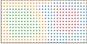
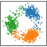
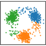
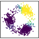
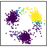
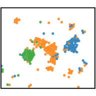
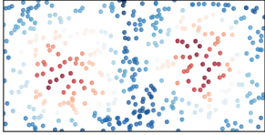
The fields of computer vision and image processing have long been concerned with the problem of recovering dynamical information (motion) from sequences of images, for an overview see Becker et al. (2014). Optical flow and motion segmentation are just two of them, which can be used to build a coherence analysis upon. Our main goal—and contribution—is to show that the theories (and state of the art computation) of optimal transport (OT) and of coherent sets are naturally connected. Fig. 1 shows a segmentation example based on our findings, see Subsection 8.4. Throughout this paper, we choose intentionally a level of detail on which this connection can be emphasized in a largely self-contained manner.
In a nutshell, we construct Frobenius–Perron operators from transport plans of (unbalanced) regularized optimal transport and use them to find coherent sets in evolving densities or particle ensembles. Such transport plans can be interpreted as small random perturbations of deterministic maps, naturally introducing a small amount of “noise” that is used for the definition of coherence (Froyland, 2013). Moreover, regularized optimal transport is an optimal choice in the sense that it yields a kind of most likely transport plan, given all that we know of the dynamics is how it maps a single distribution from an initial to a final time and that particles move according to Brownian motion.
The outline of this paper is as follows: In Section 2, we recall basic notions from measure theory, and in Section 3, we introduce properties of OT, regularized OT and unbalanced regularized OT. The segmentation model under consideration and the corresponding optimization problem as well as its relaxation are presented in Section 4. Section 5 deals with Frobenius–Perron transfer operators and the relation to OT. In particular, we construct appropriate kernels of transfer operators in two different ways, namely by i) smoothing of OT transport plans, and ii) by using regularized OT plans, where the smoothing is already inherent. Both in i) and ii) the kernels converge to the OT plan if the smoothing parameter goes to zero. As we point out in Section 6, the usage of regularized OT plans can be motivated from a statistical physics perspective. To this end, we give accessible insights, namely just for two time steps, for the Schrödinger question. We outline a discrete numerical approach in Section 7. Various proof-of-concept examples are presented in Section 8. Finally, in Section 9, conclusions are drawn.
2 Preliminaries
Throughout this paper, let be compact sets equipped with the Borel -algebras , induced by the subspace topology, respectively. Assume that the boundaries have Lebesgue measure (denoted by ) zero and that the sets fulfill for every and
| (2.1) |
for some , with balls in the appropriate spaces. This condition holds for domains satisfying the uniform cone condition, see Adams & Fournier (2003), which is fulfilled if and have Lipschitz boundaries. By we denote the linear space of all finite signed Borel measures on , by the subset of non-negative measures, and by the set of Borel probability measures on . The closed set is called the support of a measure . Further, the total variation measure of is defined by
Equipped with the norm the space becomes a Banach space. By we denote the Banach space of continuous, real-valued functions on with norm . The space can be identified via Riesz’ representation theorem with the dual space of and the weak- topology on gives rise to the weak convergence of measures, i.e., a sequence converges weakly to and we write , if
| (2.2) |
Note that the set is weakly compact.
For a non-negative, finite measure and , let be the Banach space (of equivalence classes) of complex-valued functions with norm
For the Hilbert space we use the notation . By we denote the characteristic function of a (measurable) set , defined by
Let be a sub--algebra. A mapping is called conditional expectation of if is -measurable and for all it holds
| (2.3) |
In this case, we write .
A measure is absolutely continuous with respect to , abbreviated by , if for every with we have . If satisfy , then the Radon–Nikodym derivative exists and .
Let be a measurable function, i.e., for all . Then, the push-forward measure of by is defined as . A measurable function on is integrable with respect to if and only if the composition is integrable with respect to the measure . In this case, the integrals coincide, i.e., it holds
| (2.4) |
For the Lebesgue measure , we abbreviate instead of throughout the paper.
3 Optimal Transport and its Regularization
In this section, we collect results on OT and its regularized version by the Kullback–Leibler divergence, which we couple with so-called Frobenius–Perron operators in order to segment images in the subsequent sections. Moreover, we describe unbalanced OT, which appears to be useful in our numerical examples. The following discussion is based on Cuturi & Peyré (2019) and Santambrogio (2015).
Optimal Transport
For a non-negative, symmetric and Lipschitz continuous cost function and given measures , the Monge problem of optimal transport consists in finding a measurable function , called optimal transport map, that realizes
| (3.1) |
If a map solely fulfills , we call it a transport map between and . In contrast to Monge’s problem, Kantorovich’s relaxation allows the mass to be split, i.e., it aims to find a minimizer of
| (3.2) |
where denotes the set of all joint probability measures on with marginals and . We refer to the measures of as transport plans between and . In our setting, the OT functional is continuous and (3.2) has a solution , called optimal transport plan. Every transport map between and induces a transport plan , i.e.,
Further, the -transform of is defined as and a function is called -concave if it is the -transform of some function . The dual formulation of the OT problem (3.2) reads
| (3.3) |
Maximizing pairs are of the form for a -concave function and fulfill in , where is any optimal transport plan. The function is called (Kantorovich) potential for the couple . In our applications, we want to focus on settings, where an optimal transport map exists. The following theorem can be found, e.g., in Santambrogio (2015, Thm. 1.17).
Theorem 3.1.
Let , where is absolutely continuous with respect to the Lebesgue measure and let with a strictly convex function . Then, there exists a unique optimal transport plan that is induced by the optimal transport map . Moreover, there exists a Kantorovich potential which is linked to via .
For , , the optimal transport cost induces the -Wasserstein distance
| (3.4) |
which metrizes the weak topology on . Indeed, due to boundedness of , we have that if and only if . In our numerical examples, we use the Wasserstein-2 distance. By Theorem 3.1, we have in particular for that .
Regularized Optimal Transport
We recall that the Kullback–Leibler divergence is defined for by
| (3.5) |
and by otherwise. For the last two summands in (3.5) cancel each other. The Kullback–Leibler divergence is strictly convex and weakly lower-semicontinuous with respect to the first variable. For , and , the regularized OT problem is defined as
| (3.6) | ||||
| (3.7) |
A dual formulation is given in the next theorem, see Cuturi & Peyré (2019); Neumayer & Steidl (2020).
Theorem 3.2.
The (pre-)dual problem of is given by
| (3.8) |
The optimal potentials , exist and are unique on and , respectively (up to an additive constant). They are related to the optimal transport plan by
| (3.9) |
Unbalanced Optimal Transport
In practical applications, we often have to deal with noisy data. In this case, the computation of a (regularized) optimal transport plan is often unreasonable. e.g., if are positive measures such that . To resolve this issue, we can use unbalanced regularized optimal transport, which allows small deviations between the input measures and the marginals of the associated transport plan. This approach corresponds to the optimization problem
| (3.10) |
where and denote the marginals with respect to the first and second component, respectively, see Chizat et al. (2018). Similarly as in the balanced case, we can rewrite the problem in dual form
| (3.11) | ||||
| (3.12) |
and the optimal solution of the primal problem is related to the optimal solutions of the dual problem via
| (3.13) |
Further, the formal limit results in the original balanced problem. Note that the OT plan does not have marginals and . However, if is large, the marginals and of are close to the original input measures and in some sense we can interpret them as smoothed versions of those. Similarly as for regularized OT, we can use a variant of the Sinkhorn algorithm to efficiently solve the corresponding discrete problem, see Séjourné et al. (2019).
4 Segmentation Model
Following the lines of Froyland (2013), we introduce the segmentation model that we want to apply for coherent structure detection. More precisely, we use the concept of transfer operators, which are rigorously introduced in Section 5. It is sufficient to note that the transfer operator below is the adjoint of the pullback operator as an operator between the respective spaces. Further, it is a functional extension of the push-forward operator from Section 2.
Assume that we are given full information about some dynamical system by means of its linear, bounded transfer operator . Let denote the disjoint union of sets. We aim to find measurable partitions and so that it holds for that
-
•
(coherence) and
-
•
(mass conservation).
Note that the first condition readily implies . Based on these conditions, a natural model in order to find the partitions would be
| (4.1) |
trying to optimize the alignment of and in , . The expression quantifies the probability that a -distributed random initial condition, being in , is mapped by the dynamics into . Using standard arguments, see Froyland (2013) or also von Luxburg (2007) in connection with graph cuts, problem (4.1) can be rewritten as
| (4.2) |
where and . These functions fulfill
Clearly, if we could find with corresponding , the desired partition can be obtained by thresholding these functions at zero. Unfortunately, problem (4.1) or equivalently (4.2) is hard to solve, indeed NP-hard in its finite dimensional variant. Instead, we relax the problem by replacing with and with . Then, the relaxed problem
| (4.3) |
allows for fuzzy instead of hard assignments. In the following, we set and assume that
-
(A1)
;
-
(A2)
, which by (A1) is equivalent to , where we abbreviate for the operator norm;
-
(A3)
is compact and the largest eigenvalue of is simple.
Then, problem (4.3) is equivalent to finding the second largest singular value of and the corresponding left and right singular vectors. This can be seen as follows: The compact, self-adjoint, positive operator has a non-negative spectrum, where the countable set of eigenvalues of fulfills the Courant’s minimax principle (Birman & Solomjak, 1987, Thm. 4, p. 212),
Using the definition of the norm, this can be rewritten as
| (4.4) |
The values are the non-zero singular values of , and the maximizing functions and are so-called left and right singular vectors of belonging to , respectively. Note that the left singular vectors are the eigenvectors of and right singular vectors are given by . By assumptions (A2) and (A3), is an eigenvector of belonging to the simple, largest eigenvalue so that the eigenvectors belonging to smaller eigenvalues are perpendicular to . Thus, (4.4) becomes
| (4.5) |
where the orthogonality condition on can be added since implies : To summarize, if fulfills the assumptions (A1)–(A3), then model (4.3) can be solved by finding the left and right singular functions of belonging to the second largest singular value of . Later, we focus on compact operators arising from non-negative kernels via
Then, (A1)–(A3) are met if the following corresponding assumptions hold for :
-
(K1)
-a.e.,
-
(K2)
-a.e.
-
(K3)
The largest eigenvalue of is simple.
Remark 4.1 (Relation to graph cut segmentation).
Partitioning data using the eigenvector corresponding to the second largest eigenvalue of the so-called graph Laplacian operator, which is self-adjoint for undirected graphs, is a frequently applied method, e.g., in image processing. As illustrated by Fig. 1 in the introduction, our approach is related to dynamical data sets, and we aim to partition the sets simultaneously at different times using the singular vector pairs of a not necessarily self-adjoint transfer operator, whose construction is addressed in the next sections.
5 Frobenius–Perron Operators
In this section, we consider the so-called Frobenius–Perron operator of a measurable map . In Subsection 5.1, we will see that this transfer operator fulfills our assumptions (A1) and (A2) provided that the operator is a transport map between measures and . Unfortunately, the resulting transfer operator will be useless for our segmentation task since it has only singular values and thus it violates (A3). As a possible solution, we provide a kernel-based definition of the Frobenius–Perron operator and propose two approaches for smoothing the transport maps. The first technique is suggested in Subsection 5.2. It adds a small random perturbation to the kernel of the operator, an idea that goes back to Froyland (2013). The second approach, which we will favor in our numerical examples, uses regularized optimal transport plans.
5.1 Frobenius–Perron Operators and Transport Maps
For completeness, we introduce the Frobenius–Perron operator between two Lebesgue spaces and . Analogous results for and can be found, e.g., in Boyarsky & Góra (1997, Chap. 4) or Brin & Stuck (2002); Lasota & Mackey (1994).
Assume that is non-singular with respect to and , namely that implies for all . It is immediately clear that a transport map is non-singular with respect to and . For a non-singular, measurable map , the linear operator is called Frobenius–Perron operator of if it satisfies
| (5.1) |
In other words, the function is given for each as the density of with respect to , which exists because
i.e., . In particular, integrals are preserved . Note that often the Frobenius–Perron operator is defined as an operator just mapping from to itself, see Lasota & Mackey (1994). As is non-singular, the linear operator given by
| (5.2) |
is also well-defined. It is known as Koopman operator and the adjoint of .
Remark 5.1.
Froyland (2013) defined the Frobenius–Perron operator for a map that is non-singular with respect to the Lebesgue measure, i.e.,
| (5.3) |
For and being absolutely continuous with respect to the Lebesgue measure with densities and , respectively, a transfer operator was determined by . This implies for all that
Comparing this with (5.1), we see that for this special case our Frobenius–Perron operator coincides with the above transfer operator .
If is a transport map between and , the following proposition shows that has the properties (A1) and (A2), but unfortunately only singular values , thus violating (A3).
Proposition 5.2.
Let a measurable map fulfill and let , be defined by (5.1) and (5.2), respectively. Then, the following holds true:
-
i)
For any we have , which is the conditional expectation of with respect to the -algebra . If maps Borel sets of to those of and is also -essentially injective, i.e., there exists a measurable set with on which is injective, this simplifies to .
-
ii)
For any , the Frobenius–Perron operator, as well as its adjoint, can be restricted to and , respectively.
-
iii)
The operators satisfy and .
Proof.
i) Recall the definition of conditional expectations in (2.3). We have for any that
which implies the first claim. If the conditions for the second part are fulfilled, we can choose for any . Then, the second claim follows from
ii) Using part i) and the Jensen inequality for conditional expectations, it holds for any that
| (5.4) | ||||
| (5.5) |
and
| (5.6) |
For , we only need to consider and estimate
| (5.7) |
iii) First, we have , which readily implies . Second, we obtain by definition that . ∎
By Proposition 5.2 i), we conclude that is not suited for our segmentation problem: Since with , the leading eigenvalue of is in general not simple. Additionally, this also implies that neither nor can be compact as otherwise the identity operator would be compact. A possible remedy is to smooth the operator . To this end, we need a kernel representation of . Using the family of probability measures with given by for all , condition (5.1) can be rewritten as
| (5.8) |
Note that are the disintegrations of the transport plan that is induced by the transport map with respect to . Here, the measure-valued function is usually called the transition function.
This can be generalized to non-deterministic systems by choosing other families of probability measures. Assuming that each probability measure has the density w.r.t. with , we obtain for all by (5.8) and Fubini’s theorem
Hence, we conclude that
| (5.9) |
holds -a.e., which corresponds to the definition of the Frobenius–Perron operator for kernels, see also Klus et al. (2018). The corresponding adjoint operator is given by
In this framework, we call a transition kernel with reference measures and , to which as defined above is associated.
There is also a dynamical reason for the introduction of the transition density . In the following, we will view them as with a small random perturbation. As shown by Froyland (2013), segmentation of such perturbed dynamics yields partitions and that are robust to small noise.
5.2 Smoothed Transition Kernels
In the previous subsection, we have seen that the operators arising from transport maps fulfill only some of the required properties to serve as operators in our segmentation task. Next, we are interested in blurred kernels that fulfill (K1) and (K2) and have a nontrivial spectrum. Compared to the approach proposed by Froyland (2013), we prefer to avoid the domain padding and adapt the weights in the kernels instead. This leads to modifications of the corresponding proofs.
For and a measurable map with , we define and by
| (5.10) |
Due to (2.1), is bounded from above by . Hence, is well-defined and bounded and we can introduce a new measure via . Finally, our smoothed kernel reads as
| (5.11) |
The following proposition shows that the operator defined by
| (5.12) |
is suited for our segmentation model (4.3).
Proposition 5.3.
Proof.
The first marginal property follows directly by definition of . Further, the second one can be verified by
Further, non-negativity of follows directly by definition, and square-integrability can be checked as follows
Finally, (Folland, 1984, Thm. 6.18) implies and hence fulfills the properties (K1) and (K2). ∎
Remark 5.4.
Simplicity of the largest eigenvalue of can be shown in a similar way as in Froyland (2013, Prop. 3), e.g., for being a connected domain and being a diffeomorphism with Jacobi determinant uniformly bounded from above and below. We omit the proof here, but remark that due to compactness, the multiplicity of is finite. In case , the solution to (4.3) is and the maximizing functions are in the eigenspaces corresponding to .
In case that is a transport map, we have the following convergence behavior of and as , stating that the system associated with is a small random perturbation of , see also Khas’minskii (1963) and Kifer (1986).
Proposition 5.5.
Let and be absolutely continuous measures w.r.t. the Lebesgue measure with densities and , respectively. Assume that the densities are positive a.e. and that is continuous a.e. Let be a measurable map with and set . Then, the kernel and the measure defined with respect to satisfy and as .
Proof.
For the first claim, it suffices to show for all and with and , see Billingsley (1999, Thm. 2.8(i)). Due to our assumptions on the densities, these sets also satisfy and . Using the definition of and Fubini’s theorem, we get
Next, we define
| (5.14) |
First, we show for a.e. . Fix . Then, it holds for small enough that . Thus, we get for every such where is continuous,
and hence convergence a.e.
Next, we show a.e. For and small enough, we conclude that . If , we get for small enough that . As is non-singular, the set has Lebesgue measure zero and the claim follows.
By definition, we realize that and by (2.1) that . Now, the first assertion of the theorem follows by applying Lebesgue’s dominated convergence theorem
In order to show , it suffices to prove for all with . Repeating the same calculations as in the first part of the proof with , we obtain
∎
5.3 Kernels from Regularized OT
Having the OT results in mind, we propose to construct kernels based on regularized OT plans in (3.9), respectively in (3.13) with the properties (K1)–(K3) and to use them as kernels for transfer operators in (5.12). A motivation from statistical physics for this approach is given in Section 6. Focusing on , we use
| (5.15) |
Indeed, we can use this kernel for our segmentation problem (4.3), as the following proposition shows.
Proposition 5.6.
Proof.
Using the marginal property of , we obtain by integration that and hence
which is (K1) and similarly we show (K2). Further, it is well known, that for Lipschitz the Kantorovich potentials are Lipschitz and hence bounded on compact domains, see Neumayer & Steidl (2020, Prop. 5.7). Therefore, square-integrability and non-negativity follow directly from (3.9). Finally, the assumptions of Lemma in Froyland (2013) are fulfilled as and consequently the largest eigenvalue of is simple, i.e, (K3) holds. ∎
6 Motivation for Regularized OT Kernels from Statistical Physics
In this section, we motivate that under certain assumptions our construction of from the regularized OT plan is a reasonable choice. For these purposes, the measures and are modeled as empirical measures corresponding to a large ensemble of indistinguishable particles with time-dependent random positions , , . Then, any transition kernel choice for the transfer operator corresponds to a (joint) distribution of the particle ensemble. In the absence of any other given dynamical information, it is unclear which joint distribution to pick. Although this is unlikely to represent the true dynamics when conditioning on the given measures and , one might therefore ask what happens if one makes the “blind” generic choice that each individual particle is simply following an independent Brownian path. We show that this assumption interestingly leads precisely to the regularized optimal transport plan for the particle ensembles as a whole as the number of particles approaches infinity. Although only the time-discrete case is considered, we note that the argumentation can be generalized to Wiener processes or even arbitrary positive path measures and state spaces. Here, we refer to the survey of Léonard (2014) on Schrödinger’s question, see (6.9), and to Léonard (2010) for rigorous proofs. Our self-contained approach may be more accessible than those for the general setting.
Let the particle positions be described by i.i.d. -valued random vectors , , on a common probability space with conditional probability density
| (6.1) |
Since we assume that the particles are indistinguishable, the ensemble of particles at time can be described using a -valued random variable, in other words, a random probability measure,
| (6.2) |
Note that shall again be equipped with the weak topology and we rely on the corresponding Borel -algebra. The following proposition gives an intuition on the convergence behavior of as for such a process conditioned on starting points for which the corresponding empirical distribution converges weakly to . Note that we re-use with a slight abuse of notation.
Proposition 6.1.
For any sequence of sampled initial points with
| (6.3) |
the empirical random probability measure
converges a.s. to the constant random measure as . In other words, for a.e. realization of the random variables the associated empirical measure converges weakly to as .
Proof.
For any , the random variables , , are independent with finite variances fulfilling , so that we obtain by Kolmogorov’s strong law of large numbers (Shiryaev, 1996, p. 389) that
| (6.4) |
By (6.1), we have
so that by (6.3) and weak continuity of convolutions and , the limit in (6.4) becomes
| (6.5) | |||
| (6.6) |
Thus, assuming (6.3), we obtain the assertion. ∎
In contrast to the setting in the proposition, we assume now that the initial configuration at lies in a small Wasserstein-2 ball with radius around , and those of the observed particle distribution at in . The collective dynamical behavior of the ensemble is described by the -valued random variable
| (6.7) |
which contains more information than the two random probability measures , . We are interested in estimating the conditional probability
| (6.8) |
for large and all . For small and in the infinite particle limit, this is precisely Schrödinger’s question, that can now be stated as follows: What is the limit
| (6.9) |
Interestingly, the limiting dynamical behavior of the particles is described approximately by the regularized optimal transport plan ; more precisely, the limit above and answer to Schrödinger’s question is . However, we have to be careful here. The statement holds for the entropy regularized OT distance
| (6.10) | ||||
| (6.11) |
The relation between the KL-regularized OT in (3.6) and the entropy regularized OT in (6.10) is described in the following remark. Roughly speaking, the KL-regularized OT is more general as minimizers always exist, but there are many cases where both minimization problems coincide.
Remark 6.2.
Let and denote the densities of and , respectively. For with density the entropy is defined by . Note that if and only if for any . If , we can show for any with that it holds
| (6.12) |
Consequently, in this case the minimizer for KL-regularized OT (3.6) and entropy regularized OT (6.10) coincide. The crux is the condition , which is equivalent to having finite entropy, i.e., are in a so-called Orlicz space , see Clason et al. (2019); Navrotskaya & Rabier (2013). For more information we refer to Neumayer & Steidl (2020).
The following proposition establishes a relation between regularized optimal transport plans minimizing (6.10) and Schrödinger’s question. As already mentioned, this fact is known in a more general setting. For the sake of completeness, we add the proof for our setting.
Proposition 6.3.
Let be i.i.d. -valued random vectors on a common probability space with conditional density (6.1), and let , , and be given by (6.2) and (6.7), respectively. Then, it holds for fulfilling and every with that
| (6.13) |
where is the regularized optimal transport plan minimizing (6.10) with the Wasserstein-2 cost function.
Proof.
For , set and consider the unique minimizers , see after (3.5). Clearly, we have by (3.7) for any that
| (6.14) |
Choose a sequence , , with for . Using the weak compactness of and the weak closedness of any , we conclude that all accumulation points of are contained in for any fixed . Consequently, they are also contained in . Take a weak accumulation point using weak compactness, and with abuse of notation, choose a subsequence such that as . By weak lower-semicontinuity of , we have that
Since is a feasible point of the regularized OT problem (3.6), this implies that the whole sequence converges weakly to as . Due to (6.8), we have
| (6.15) |
Using logarithm laws and Sanov’s Theorem 6.4, see Dembo & Zeitouni (2010, Thm. 6.2.10), for the respective summands, we obtain for any measurable satisfying and –which by convergence of also implies for small enough–that
where the last inequality follows from the strict convexity of . Hence, we obtain
Using complements, we conclude for any measurable satisfying and , that
so that our claim follows from these two results using the monotonicity of measures. ∎
Theorem 6.4 (Sanov).
Let be a sequence of i.i.d. -valued random variables with distribution on some probability space, where is equipped with the weak topology. Then, it holds for any measurable with that
To summarize, in the case that the particles make independent Gaussian jumps, conditioning on initial and end configurations close to and means having a dynamical behavior of the particles described approximately by the regularized optimal transport plan .
7 Discretization
In this section, we discuss the discrete settings for our numerical computations. In Subsection 7.1, we consider the construction of smoothed transition kernels from OT plans and from entropic OT plans and illustrate their behaviour by a numerical example. Since the second approach is much more efficient, we will choose it in the numerical part. Further, we provide the corresponding segmentation algorithms in Subsection 7.2.
7.1 Discrete Kernels
In view of numerical applications, we focus now on discrete OT for the kernel construction. Let with and with be the support points of and , respectively. Then, the OT plan is given by
and similarly for the regularized OT plans. Here, can be interpreted as a mapping . For convenience, we extend all vectors and mappings to the whole integers by setting them to zero outside of the index sets and .
Smoothed Transition Kernels from OT
The construction of smoothed transition kernels as proposed in Subsection 5.2 relies on the transport map associated to the OT plan . Unfortunately, for the discrete transport problem, this OT map does not necessarily exist. Therefore, we replace the smoothed transition kernels described in Subsection 5.2 by a construction that uses transport plans instead of transport maps. Let denote some positive, normalized smoothing kernel centered around with finite width. For , we smooth in -direction to get
and set for or . The rescaling of ensures that mass is preserved, i.e.,
| (7.1) |
Next, we smooth in -direction as
and set again for or . Here, the denominator ensures that the mass is only distributed between indices and consequently, for any ,
Then, the final kernel is defined by
It is straightforward to check that this kernel fulfills (K1), and also (K2), with the smoothed marginal measure , i.e., and . Property (K3), that is, simplicity of the largest singular value of defined by (5.12), might fail in cases where has a “block-diagonal structure” and the width of is small enough for the blurred kernel to retain this structure. In this case, either needs to be increased, or one obtains “perfectly” coherent sets corresponding to the largest singular value, see Remark 5.4.
Kernels from Regularized OT
Numerical Comparison
The proposed methods for creating kernels are compared numerically for the cost .
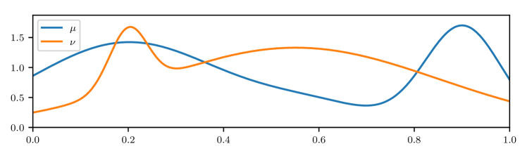
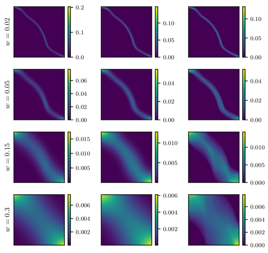
For this purpose, we fix the two probability densities and on displayed in Fig. 3, which are sums of Gaussians. The kernel proposed in (7.2) for different standard deviations is shown in the left column of Fig. 3. To get a clue about the smoothed kernel, we blur the OT plan using two different functions, namely a Gaussian kernel and an averaging blur within a ball of width , both centered around . To ensure that has finite width, we set the values below to zero. Both discrete functions are normalized, such that they sum up to one. The resulting smoothed kernels are depicted in the middle and right columns in Fig. 3. They look similar to the left ones, however, the averaging kernel appears to be artificially rough for large . As a consequence, it seems natural to use regularized OT plans instead of smoothed OT plans. Note that the cost for computing with the Sinkhorn algorithm scales with , i.e., should not be to small, see Cuturi (2013). This is not a real issue, since we need a certain amount of blur anyways in order to ensure that the leading singular value in the corresponding transfer operator is simple.
7.2 Segmentation Algorithms
In our numerical examples in the next section, we apply the kernel (7.2). However, we will see that for the addressed applications the unbalanced OT plan with corresponding kernel (7.3) leads to more natural results. In the following, we use the matrix-vector notation
and , . Further, let , , and similarly for the unbalanced kernels. Then (7.2) becomes . To solve the segmentation model (4.3), we have to find the second largest singular values of the discrete transfer operator given by
Then, the Rayleigh quotient in (4.3) can be rewritten as
| (7.4) |
where we substituted and . The constraint in (4.3) becomes
and indeed is the left singular vector to the largest singular value of . This holds also accordingly for the dominant right singular vector. To compute the singular vectors belonging to the largest singular values of this matrix, we apply a (truncated) singular value decomposition (SVD). We summarize our steps in Algorithm 1. Readers familiar with Froyland et al. (2010) will notice the evident analogies between our algorithm and Froyland et al. (2010, Lem. 1) in computing the segmentation (coherent sets). The transition matrix therein connects to the objects used by us via . If the marginal requirement on and is not fulfilled, unbalanced OT may be preferable. Similarly as above, the same considerations for unbalanced regularized OT lead to Algorithm 2.
Remark 7.1 (Multiphase Segmentation).
In our numerical examples, we are also interested in partitions with more than just two sets. These can be obtained by using additional singular functions as it is also known in the extensive literature on graph cut partitions, see, e.g., von Luxburg (2007). To this end, we employ the maximizers of the problem
| (7.5) |
where are the solutions of (4.3), i.e., the second largest singular vector pair. It is not hard to show that the solutions of (7.5) are given by the singular functions corresponding to the third largest singular value of . Similarly, we can consider further singular function pairs. Based on these singular functions, we compute a multiphase partition using the -means (or fuzzy -means) algorithm.
8 Numerical Results
In this section, we present various examples. All involved transport plans are computed with respect to the squared Euclidean distance as cost function.
8.1 Exploring Coherent Set Detection

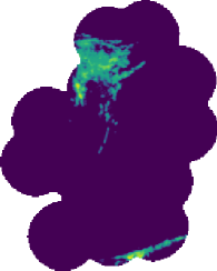
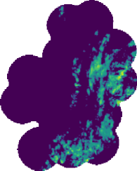
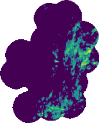
First, we apply our method to a data set of precipitation densities over Germany, which was made freely available by Winterrath et al. (2018). We take two pairs of snapshots, see Fig. 4. In order to cope with memory limitations, we have applied spatial averaging and masked out all indices with or , resulting in the problem dimensions for Fig. 4a, for Fig. 4b, for Fig. 4c and for Fig. 4d. In Figs. 4a–4b, we clearly see two main areas of precipitation: One in the north west, and another one in the south east. Since these two areas do not move much, it should be easy to identify them as coherent sets. In the second example, it is less obvious what the optimal partition should be. Both discrete densities and are normalized such that . Now, we can apply our proposed procedure from Section 7: First, we compute the regularized optimal transport plan with regularization parameter using the Python Optimal Transport package (POT)111Code available at https://github.com/rflamary/POT (accessed: 26.06.2020), where the distance between two neighboring pixels is . Then, we compute the singular vectors and of the matrix as well as the optimal partition vectors and . Numerically, we observe that choosing small produces partition functions that are almost constant on the respective parts with a sharp transition between them, whereas very large yields approximately affine partition functions, which is clearly not what we want. In any case, has to be chosen large enough such that the Sinkhorn algorithm converges in acceptable time.


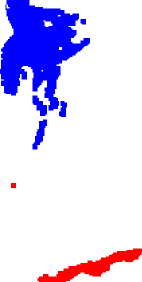


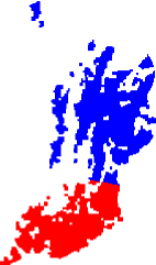
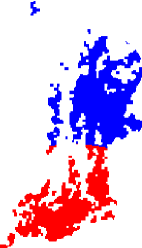
Results are shown in Fig. 7. Note that the dark-blue pixels in Fig. 4 are only included to indicate the domain of and and not part of the computation. Hence, they are discarded in Figs. 7–7. We observe that the method works roughly as expected: As shown in our theory part, the first singular value is one and belongs to the singular pair . Further, the two precipitation areas are indicated by differing signs in the partition vectors corresponding to the second singular value. However, taking a closer look, splitting the precipitation areas (or “fuzzy classification”) does not work perfectly. In Fig. 7, some parts of the bigger “cloud” (as we refer to precipitation areas from now on) have values greater than zero, although the rest has negative values. Ceonsequently, some parts of the upper cloud are classified as “red”, i.e., as part of the lower cloud. This issue is even more pronounced for the included hard “classification” according to the criteria and . Note that simple thresholding was sufficient for our purposes, but more sophisticated approaches such as fuzzy -means (which will be used in the next subsection) or sparsity-promoting clustering, see Froyland et al. (2019), are also applicable.
Next, we want to resolve the mentioned issue of wrong classification. Of course, it is inaccurate to model precipitation densities as transported mass particles, since they can come down as rain and simply disappear. Hence, the misclassification is not surprising as the OT plan needs to transport this disappearing mass somewhere else. Indeed, an examination of the transport plan reveals that mass preservation does not hold in the two clouds, thus they cannot fulfill the coherence condition (see Section 4) and the transport needs to shift some of the mass from the upper cloud to the lower one.
To compensate for this effect, we propose to use unbalanced regularized OT, relaxing the mass conservation condition on the marginals, see Section 3. Noteworthy, this modification does not introduce any major computational overhead. Again, we use and choose , see (3.10). As mentioned by Séjourné et al. (2019), the parameter intuitively corresponds to a choice of radius for which, when exceeded, it is cheaper to produce or destroy mass instead of transporting it between the two clouds. Hence, we should choose small enough to have an effect compared to balanced OT, but large enough so that the marginals of the resulting transport plan are still close to the given and .
The results for the data from Figs. 4a–4b and Figs. 4c–4d are displayed in Figs. 7 and 7, respectively. As expected, the first singular pair is still given by . Now, the area classification in Figs. 4a–4b is more or less perfect and hence also the second singular value is almost one. This might not be surprising, as the areas are well separated and moving mass between them is quite expensive. Compared to standard regularized transport, using unbalanced regularized transport for the data from Figs. 4c–4d does not change the partition much. Overall, the results based on unbalanced regularized OT look very promising and hence we use such plans in all further experiments. Note that a comparison with the coherent set methods mentioned in Section 1 is not possible, since these require a known dynamic.
8.2 Particles Moving in a Potential
In this subsection, we discuss the example of Koltai et al. (2018, Sec. 6.2, p. 18) in a slightly modified form. The dynamical system under consideration consists of particles moving according to standard Brownian motion with a drift term induced by a potential and a rotating force. More precisely, our particle trajectories are solutions to the stochastic differential equation
where denotes standard Brownian motion, is the force coming from the -well potential
and is a circular driving force in clock-wise direction, given by
In statistical physics, is called inverse temperature, which is chosen as in this experiment. Note that is strongest in the valley of each well. Overall, the particles tend to remain in a well for some time and occasionally hop to another one due to their diffusive motion and the circular force. We expect the particle distribution to converge to an equilibrium with modes at the potential minima, slightly rotated in clock-wise direction.
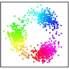
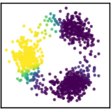
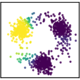
First, we create initial particle positions for the measure as follows: We sample a single-particle-trajectory with steps of time length using an Euler–Maruyama-scheme starting from , where the circular driving force is neglected. Then, we draw trajectory points uniformly at random from these points without replacement. The final discrete measure is simulated by the numerical trajectories for each one of these initial particle positions using Euler–Maruyama-steps of length , where is included now. This yields pairs of starting and ending position displayed in Fig. 10. To visualize the trajectory of individual particles, we colored each particle in Fig. 8b in the same color as in Fig. 8a. Further, in Fig. 8c, we drew connecting lines between initial and terminal particle positions.
Next, we apply Algorithm 2 to and with . The regularization parameter is chosen so that the corresponding kernel (see (3.7)) has standard deviation one third of the particles mean distance at . We write and for the partition vectors belonging to the decreasingly ordered singular values , where and are the corresponding left and right singular vectors. The obtained partition vector pairs for are shown in Fig. 10.
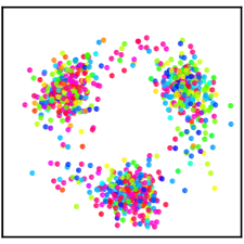
Using the information from , , we can embed every point into via , . Now, we partition the data using the fuzzy -means algorithm222Implementation available at https://github.com/omadson/fuzzy-c-means (accessed: 26.06.2020) as described in Sec. 4 on this embedded data for three clusters, see also Shafei & Steidl (2012). In contrast to applying fuzzy -means directly on the individual snapshots at , we naturally obtain correspondences between the clusters at the different time steps, where OT serves as a proxy for the underlying dynamics. The obtained hard clusters and fuzzy membership values are displayed in Fig. 10.
Note that applying the method in Froyland (2013) under usage of the particle label information cannot yield coherent sets for such strong particle mixing. Other methods such as the finite-time Lyapunov exponent (Shadden et al., 2005) also only work for short timespans. On the other hand, comparing this with our method, it is clear from Fig. 10 that the OT assignment will be very different from the ground truth particle correspondences. Thus, it aims for a partition based on the “macroscopic”, ensemble density level rather than on the “microscopic” level of individual, distinguishable particles. Indeed, we observe that the coherent sets are three denser blobs due to the energy landscape. Since there was no circular force present during the construction of , there is a slight offset between the initial and stationary distributions, which is captured by the coherent sets. As expected, the likeliness of being in a cluster decreases if a point is close to the boundaries of the well. Consequently, there is some uncertainty about the exact cluster boundaries.


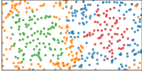
8.3 Particles with Pairwise Lennart–Jones Potentials
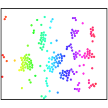
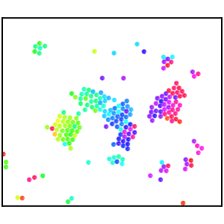
In the last example, we aim for a segmentation of particle groups with a slightly more realistic data set, consisting of particle trajectories created with the molecular dynamics simulation software LAMMPS (Plimpton, 1993). In our simulation, the particles interact with each other in terms of a pairwise Lennart–Jones potential with cutoff, essentially repelling each other in close proximity but attracting each other otherwise, such that there is some optimal energy-minimizing pairwise distance (Rapaport, 2004). Given some initial velocity for the particles, they start to stick to each other over time and slowly form groups, which in turn connect to larger groups and so on. We take two snapshots of the simulation showing some group formation, see Fig. 13. As the domain is the two-dimensional torus, particles leaving the domain on one side come back in from the opposite side in the visualization. 333The script for generating the trajectories is available at the blog post under http://nznano.blogspot.com/2017/11/molecular-dynamics-in-python.html#Implementation-in-LAMMPS (accessed: 26.06.2020)
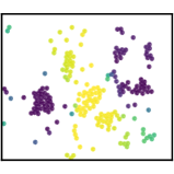
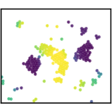
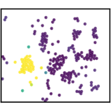
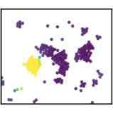
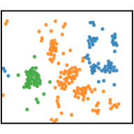
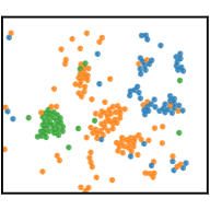
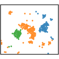
Then, we apply our computational scheme with the same parameter choices as in Subsection 8.2 to obtain the clusters. The computed segmentation vectors and the induced fuzzy clustering are depicted in Figs. 13 and 13, respectively. From a visual point of view, the clustering scheme “correctly” detects the stable group on the left, roughly three connecting groups in the middle and several smaller connecting groups on the right, independent of the mixing of several individual particles.
As we obtained the data by a molecular dynamics simulation, we can access the “ground truth” particle labels and track the position of every particle forward and backward in time. Since the particle mixing in this example is not as strong as in Section 8.2, it is natural to ask whether the hard cluster labels of particle are the same at . We observe that the cluster labels agree in of the total cases, that is, around of the particles retain their cluster label in time. Furthermore, we may compare the hard cluster label of each particle at time with the one that particle is assigned at time in two scatter plots, where the position in the plot of each particle is fixed and the two different colorings indicate the hard cluster labels for and (that is, corresponding to the left or right singular vectors), respectively. The results are shown in Fig. 14.

8.4 Particle Tracking with Concatenated Transfer Operators
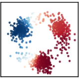
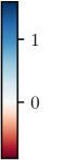
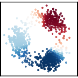
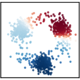
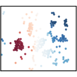
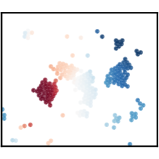
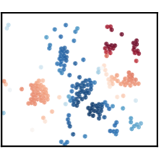
Here, we discuss an example also analyzed by Froyland & Padberg-Gehle (2014b) and Banisch & Koltai (2017, Sec. V.A). Consider the non-autonomous system
| (8.1) | ||||
with and parameters , and . This system describes two counter-rotating gyres, where the vertical boundary between them oscillates periodically. Moreover, it preserves the Lebesgue measure on .
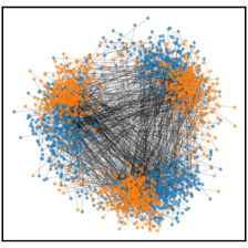
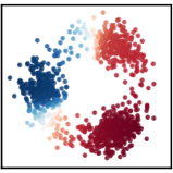
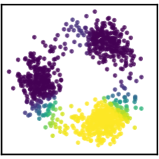
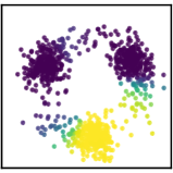
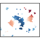
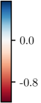
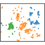
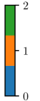
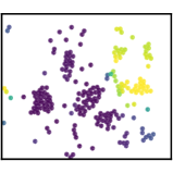
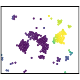
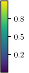
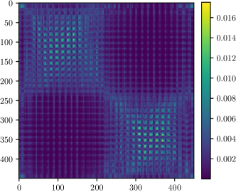
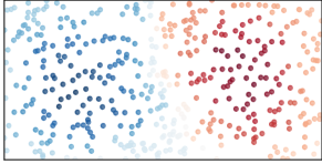
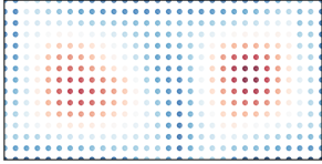
We initialize particles on an equispaced rectangular grid. Then, we compute their trajectories by solving (8.1) with time steps of length , i.e., on the time interval . This yields measures , . Note that is small enough to recover the ground truth particle correspondences in most cases. Based on the entropy regularized optimal transport plans between and with regularization parameter , we construct corresponding transfer operators as . Again, the entropy regularization readily introduces the required diffusion. Efficient implementations of the Sinkhorn algorithm can be achieved using, e.g., multiscale schemes (Schmitzer, 2019) or parallelization on GPUs (Cuturi, 2013). Next, we compute the concatenated transfer operator , for which its matrix is shown in Fig. 16. Its block-diagonal structure already indicates coherent sets. Finally, the partitions corresponding to the second and third singular vectors , , , of its SVD are shown in Fig. 16. The corresponding singular values are and , respectively. For a hard clustering using fuzzy -means we refer to Fig. 1 in the introduction.
Particle transitions between the left and the right half of the domain are very rare, as indicated by the optimal partition. Further, the third singular vectors illustrate that the particles, which move in closed curves around the respective gyre cores, take a long time to transition from the gyre centers to their boundaries or vice versa. In summary, this example illustrates how our method can be used to compute coherent sets for flows with unlabeled particles. Here, OT is used to track them through observations of subsequent timesteps; see also Particle Image Velocimetry (Saumier et al., 2015).


9 Conclusions
This is the first paper that merges the theories of Frobenius–Perron operators and regularized optimal transport. We have elaborated how regularized (and possibly unbalanced) OT can be used to compute coherent sets if all we know about the dynamics of a moving particle system or a continuous quantity of moving mass is a pair of measures that constitute a preimage-image pair under the dynamical evolution. We have also shown that the theory of (regularized/unbalanced) optimal transport is fitting well to the concept of coherent sets. Moreover, it has natural dynamical interpretations as the regularization parameter or the number of data points , see Proposition 5.7 and Proposition 6.3, respectively.
In four numerical examples we have shown how the method performs. These examples underline the initial suspicion that without further structural “aid” or dynamic information the knowledge of the one-step evolution of a single measure is not sufficient to identify coherent sets correctly. It is necessary to incorporate additional dynamical information into the analysis. Thus, a topic interesting to address is OT of multiple measure pairs (multiple steps of evolving one measure, or one step of evolving multiple measures), such as in segmentation of vector- and manifold-valued images, see, e.g., Chen et al. (2018); Fitschen et al. (2016, 2017); Kushinsky et al. (2019); Thorpe et al. (2017). Further, working with discrete OT calls for a consistency result when approximating ground truth measures with atomic ones, as it has been given for the case of (static) spectral clustering in García Trillos & Slepčev (2018) using transportation distances between functions as provided in the aforementioned references. Finally, the efficacy of unbalanced OT suggests to model certain scenarios as open dynamical systems.
Acknowledgments
Funding through the German Research Foundation (DFG) within the project STE 571/16-1 is gratefully acknowledged by GS, through grant CRC 1114 “Scaling Cascades in Complex Systems”, Project Number 235221301, projects A01 “Coupling a multiscale stochastic precipitation model to large scale atmospheric flow dynamics” by PK and B07 “Selfsimilar structures in turbulent flows and the construction of LES closures” by JvL. The authors want to thank Henning Rust, Institute for Meteorology at FU Berlin, for his advice regarding the data of the example from Section 8.1.
References
- Adams & Fournier (2003) Adams, R. & Fournier, J. (2003) Sobolev Spaces. Pure and Applied Mathematics, vol. 140, second edn. Amsterdam: Elsevier/Academic Press, pp. xiv+305.
- AlMomani & Bollt (2018) AlMomani, A. & Bollt, E. (2018) Go with the flow, on Jupiter and snow. Coherence from model-free video data without trajectories. J. Nonlinear Sci., 1–30.
- Aref (2002) Aref, H. (2002) The development of chaotic advection. Phys. Fluids, 14, 1315–1325.
- Banisch & Koltai (2017) Banisch, R. & Koltai, P. (2017) Understanding the geometry of transport: diffusion maps for Lagrangian trajectory data unravel coherent sets. Chaos, 27, 035804, 16.
- Becker et al. (2014) Becker, F., Petra, S. & Schnörr, C. (2014) Optical Flow. Handbook of Mathematical Methods in Imaging (O. Scherzer ed.). New York: Springer.
- Billingsley (1999) Billingsley, P. (1999) Convergence of Probability Measures. Wiley Series in Probability and Statistics, second edn. New York: John Wiley, pp. x+277.
- Birman & Solomjak (1987) Birman, M. S. & Solomjak, M. Z. (1987) Spectral Theory of Selfadjoint Operators in Hilbert Space. Mathematics and its Applications. Dordrecht: Springer Netherlands, pp. xv+301.
- Boyarsky & Góra (1997) Boyarsky, A. & Góra, P. (1997) Laws of Chaos. Probability and its Applications. Boston: Birkhäuser Boston, pp. xvi+399.
- Brin & Stuck (2002) Brin, M. & Stuck, G. (2002) Introduction to Dynamical Systems. Cambridge: Cambridge University Press, pp. xii+240.
- Carlier et al. (2017) Carlier, G., Duval, V., Peyré, G. & Schmitzer, B. (2017) Convergence of entropic schemes for optimal transport and gradient flows. SIAM J. Math. Anal., 49, 1385–1418.
- Chen et al. (2018) Chen, Y., Tryohon, T. G. & Tannenbaum, A. (2018) Vector-valued optimal mass transport. SIAM J. Appl. Math., 78, 1682–1696.
- Chizat et al. (2018) Chizat, L., Peyré, G., Schmitzer, B. & Vialard, F.-X. (2018) Scaling algorithms for unbalanced optimal transport problems. Math. Comput., 87, 2563–2609.
- Clason et al. (2019) Clason, C., Lorenz, D. A., Mahler, H. & Wirth, B. (2019) Entropic regularization of continuous optimal transport problems. arXiv e-prints, arXiv:1906.01333.
- Cuturi (2013) Cuturi, M. (2013) Sinkhorn distances: Lightspeed computation of optimal transport. Advances in Neural Information Processing Systems (C. J. C. Burges, L. Bottou, M. Welling, Z. Ghahramani & K. Q. Weinberger eds), vol. 26. New York: Curran Associates, pp. 2292–2300.
- Cuturi & Peyré (2019) Cuturi, M. & Peyré, G. (2019) Computational optimal transport. Found. Trends Mach. Learn., 11, 355–607.
- Dembo & Zeitouni (2010) Dembo, A. & Zeitouni, O. (2010) Large Deviations Techniques and Applications. Stochastic Modelling and Applied Probability, vol. 38. Berlin: Springer, pp. xvi+396.
- Feydy et al. (2019) Feydy, J., Séjourné, T., Vialard, F.-X., Amari, S., Trouvé, A. & Peyré, G. (2019) Interpolating between optimal transport and MMD using Sinkhorn divergences. Proceedings of Machine Learning Research, vol. 89. PMLR, pp. 2681–2690.
- Fitschen et al. (2016) Fitschen, J. H., Laus, F. & Steidl, G. (2016) Transport between RGB images motivated by dynamic optimal transport. J. Math. Imaging Vision, 56, 409–429.
- Fitschen et al. (2017) Fitschen, J. H., Laus, F. & Schmitzer, B. (2017) Generalized optimal transport for manifold-valued images. Scale Space and Variational Methods in Computer Vision. Springer International Publishing, pp. 460–472.
- Folland (1984) Folland, G. B. (1984) Real Analysis. New York: J. Wiley.
- Froyland et al. (2010) Froyland, G., Santitissadeekorn, N. & Monahan, A. (2010) Transport in time-dependent dynamical systems: Finite-time coherent sets. Chaos, 20, 043116.
- Froyland (2013) Froyland, G. (2013) An analytic framework for identifying finite-time coherent sets in time-dependent dynamical systems. Phys. D, 250, 1–19.
- Froyland et al. (2019) Froyland, G., Rock, C. P. & Sakellariou, K. (2019) Sparse eigenbasis approximation: Multiple feature extraction across spatiotemporal scales with application to coherent set identification. Commun. Nonlinear Sci. Numer. Simul., 77, 81–107.
- Froyland & Padberg (2009) Froyland, G. & Padberg, K. (2009) Almost-invariant sets and invariant manifolds – connecting probabilistic and geometric descriptions of coherent structures in flows. Phys. D, 238, 1507–1523.
- Froyland & Padberg-Gehle (2014a) Froyland, G. & Padberg-Gehle, K. (2014a) Almost-invariant and finite-time coherent sets: directionality, duration, and diffusion. Ergodic theory, open dynamics, and coherent structures. Springer Proc. Math. Stat., vol. 70. New York: Springer, pp. 171–216.
- Froyland & Padberg-Gehle (2014b) Froyland, G. & Padberg-Gehle, K. (2014b) Almost-invariant and finite-time coherent sets: directionality, duration, and diffusion. Ergodic theory, open dynamics, and coherent structures. Springer Proc. Math. Stat., vol. 70. New York: Springer, pp. 171–216.
- García Trillos & Slepčev (2018) García Trillos, N. & Slepčev, D. (2018) A variational approach to the consistency of spectral clustering. Appl. Comput. Harmon. Anal., 45, 239–281.
- Hadjighasem et al. (2017) Hadjighasem, A., Farazmand, M., Blazevski, D., Froyland, G. & Haller, G. (2017) A critical comparison of Lagrangian methods for coherent structure detection. Chaos, 27, 053104.
- Hadjighasem & Haller (2016) Hadjighasem, A. & Haller, G. (2016) Geodesic transport barriers in Jupiter’s atmosphere: A video-based analysis. SIAM Rev., 58, 69–89.
- Haller et al. (2018) Haller, G., Karrasch, D. & Kogelbauer, F. (2018) Material barriers to diffusive and stochastic transport. Proc. Natl. Acad. Sci. USA, 115, 9074–9079.
- Haller & Poje (1998) Haller, G. & Poje, A. C. (1998) Finite time transport in aperiodic flows. Phys. D, 119, 352–380.
- Jones & Winkler (2002) Jones, C. & Winkler, S. (2002) Invariant manifolds and Lagrangian dynamics in the ocean and atmosphere. Handbook of Dynamical Systems, vol. 2. Amsterdam: North-Holland, pp. 55–92.
- Karrasch & Keller (2020) Karrasch, D. & Keller, J. (2020) A geometric heat-flow theory of Lagrangian coherent structures. J. Nonlinear Sci., 30, 1849–1888.
- Khas’minskii (1963) Khas’minskii, R. Z. (1963) Principle of averaging for parabolic and elliptic differential equations and for Markov processes with small diffusion. Theor. Probab. Appl., 8, 1–21.
- Kifer (1986) Kifer, Y. (1986) General random perturbations of hyperbolic and expanding transformations. J. d’Analyse Math., 47, 111–150.
- Klus et al. (2018) Klus, S., Nüske, F., Koltai, P., Wu, H., Kevrekidis, I., Schütte, C. & Noé, F. (2018) Data-driven model reduction and transfer operator approximation. J. Nonlinear Sci., 28, 985–1010.
- Koltai et al. (2018) Koltai, P., Wu, H., Noé, F. & Schütte, C. (2018) Optimal data-driven estimation of generalized Markov state models for non-equilibrium dynamics. Computation, 6, 22.
- Koltai & Renger (2018) Koltai, P. & Renger, D. M. (2018) From large deviations to semidistances of transport and mixing: coherence analysis for finite Lagrangian data. J. Nonlinear Sci., 28, 1915–1957.
- Kushinsky et al. (2019) Kushinsky, Y., Maron, H., Dym, N. & Lipman, Y. (2019) Sinkhorn algorithm for lifted assignment problems. SIAM J. Imag. Sci., 12, 716–735.
- Lasota & Mackey (1994) Lasota, A. & Mackey, M. (1994) Chaos, Fractals, and Noise: Stochastic Aspects of Dynamics. Applied Mathematical Sciences, vol. 97, second edn. New York: Springer, pp. xiv+472.
- Léonard (2010) Léonard, C. (2010) Entropic projections and dominating points. ESAIM Probab. Stat., 14, 343–381.
- Léonard (2014) Léonard, C. (2014) A survey of the Schrödinger problem and some of its connections with optimal transport. Discrete Contin. Dyn. Syst., 34, 1533–1574.
- Navrotskaya & Rabier (2013) Navrotskaya, I. & Rabier, P. (2013) and finite entropy. Adv. Nonlinear Anal., 2, 379–387.
- Neumayer & Steidl (2020) Neumayer, S. & Steidl, G. (2020) From optimal transport to discrepancy. arXiv e-prints, arXiv:2002.01189.
- Plimpton (1993) Plimpton, S. (1993) Fast parallel algorithms for short-range molecular dynamics. Technical Report. Albuquerque, NM (United States): Sandia National Labs.
- Rapaport (2004) Rapaport, D. (2004) The Art of Molecular Dynamics Simulation. Cambridge: Cambridge University Press.
- Rom-Kedar et al. (1990) Rom-Kedar, V., Leonard, A. & Wiggins, S. (1990) An analytical study of transport, mixing and chaos in an unsteady vortical flow. J. Fluid Mech., 214, 347–394.
- Santambrogio (2015) Santambrogio, F. (2015) Optimal Transport for Applied Mathematicians. Progress in Nonlinear Differential Equations and their Applications, vol. 87. Cham: Birkhäuser/Springer, pp. xxvii+353.
- Santitissadeekorn & Bollt (2020) Santitissadeekorn, N. & Bollt, E. M. (2020) Ensemble-based method for the inverse Frobenius-Perron operator problem: data-driven global analysis from spatiotemporal “movie” data. Phys. D, 411, 132603.
- Saumier et al. (2015) Saumier, L.-P., Khouider, B. & Agueh, M. (2015) Optimal transport for particle image velocimetry. Commun. Math. Sci., 13, 269–296.
- Schmitzer (2019) Schmitzer, B. (2019) Stabilized sparse scaling algorithms for entropy regularized transport problems. SIAM J. Sci. Comput., 41, A1443–A1481.
- Séjourné et al. (2019) Séjourné, T., Feydy, J., Vialard, F.-X., Trouvé, A. & Peyré, G. (2019) Sinkhorn Divergences for Unbalanced Optimal Transport. arXiv e-prints, arXiv:1910.12958.
- Shadden et al. (2005) Shadden, S. C., Lekien, F. & Marsden, J. E. (2005) Definition and properties of Lagrangian coherent structures from finite-time Lyapunov exponents in two-dimensional aperiodic flows. Phys. D, 212, 271–304.
- Shafei & Steidl (2012) Shafei, B. & Steidl, G. (2012) Segmentation of images with separating layers by fuzzy c-means and convex optimization. J. Visual Commun. Image Represent., 3, 611–621.
- Shiryaev (1996) Shiryaev, A. N. (1996) Probability. Graduate Texts in Mathematics, vol. 95, second edn. New York: Springer, pp. xvi+623. Translated from the first (1980) Russian edition by R. P. Boas.
- Thiffeault (2012) Thiffeault, J.-L. (2012) Using multiscale norms to quantify mixing and transport. Nonlinearity, 25.
- Thorpe et al. (2017) Thorpe, M., Park, S., Kolouri, S., Rohde, G. K. & Slepčev, D. (2017) A transportation distance for signal analysis. J. Math. Imaging Vision, 59, 187–210.
- von Luxburg (2007) von Luxburg, U. (2007) A tutorial on spectral clustering. Stat. Comput., 17, 395–416.
- Wiggins (1992) Wiggins, S. (1992) Chaotic Transport in Dynamical Systems. New York: Springer.
- Wiggins (2005) Wiggins, S. (2005) The dynamical systems approach to Lagrangian transport in oceanic flows. Annu. Rev. Fluid Mech., 37, 295–328.
- Winterrath et al. (2018) Winterrath, T., Brendel, C., Hafer, M., Junghänel, T., Klameth, A., Lengfeld, K., Walawender, E., Weigl, E. & Becker, A. (2018) Radklim version 2017.002: Reprocessed quasi gauge-adjusted radar data, 5-minute precipitation sums (yw).