Modeling and Computation of High Efficiency and Efficacy Multi-Step Batch Testing for Infectious Diseases

Abstract

We propose a mathematical model based on probability theory to optimize COVID-19 testing by a multi-step batch testing approach with variable batch sizes. This model and simulation tool dramatically increase the efficiency and efficacy of the tests in a large population at a low cost, particularly when the infection rate is low. The proposed method combines statistical modeling with numerical methods to solve nonlinear equations and obtain optimal batch sizes at each step of tests, with the flexibility to incorporate geographic and demographic information. In theory, this method substantially improves the false positive rate and positive predictive value as well. We also conducted a Monte Carlo simulation to verify this theory. Our simulation results show that our method significantly reduces the false negative rate. More accurate assessment can be made if the dilution effect or other practical factors are taken into consideration. The proposed method will be particularly useful for the early detection of infectious diseases and prevention of future pandemics. The proposed work will have broader impacts on medical testing for contagious diseases in general.
Key Words: Coronavirus; COVID-19; False negative rate; Pandemic; PCR test; Sample pooling

1 Introduction

To fight the COVID-19 pandemic with limited resources, batch tests were recommended by pooling multiple swab samples. Samples from different individuals are pooled into one batch and then a high-throughput PCR test is conducted (Cheng, 2020; Lohse et al., 2020; Shani-Narkiss et al., 2020). If the batch is tested negative, then it can be deduced that all samples were negative. Otherwise, each sample needs to be tested individually. Pooling data was originally proposed by Dorfman (1943) for detecting syphilis in US soldiers during World War II. Farrington (1992), Gastwirth and Hammick (1989), Chen and Swallow (1990), Gastwirth and Johnson (1994), Hardwick et al. (1998), Hung and Swallow (2000), Vansteelandt et al. (2000), Xie (2001), Bilder and Tebbs (2009) and Chen et al. (2009) developed group-testing regression on parametric models. Delaigle and Meister (2011) developed a nonparametric method to estimate the conditional probability of contamination for pooled data. Wang, McMahan et al. (2014) developed semiparametric group testing regression models. France et al. (2015) used pooling samples to reduce the number of tests required for detection of anthrax spores. Kline et al. (1989), Behets et al. (1990), Lindan et al. (2005), Pilcher et al. (2005), Hourfar et al. (2008), Stramer et al. (2013) and Warasi et al. (2016) developed group testing methods to screen sexually transmitted diseases. Pooled samples were used to detect other infectious diseases in Busch et al. (2005), Van et al. (2012) and Wang, Han et al. (2014). Nagi and Raggi (1972), Fahey et al. (2006), Wahed et al. (2006) and Lennon (2007) pooled observations to test for contamination by a toxic substance. Huang (2009) and Huang and Tebbs (2009) studied measurement error models for group testing data.

By grouping individuals, batch testing significantly reduces the number of tests, providing an efficient method to detect community transmission (Hogan et al., 2020). Batch testing has become more relevant recently, as state and local governments seek to test as many people as possible to transition safely back to normal life. In July 2020, the US Food and Drug Administration issued emergency authorization for sample pooling in diagnostic testing (US Food and Drug Administration, 2020). Places abroad such as South Korea have been using pooling methods to sample in batches of a fixed size in high-risk communities (Park and Koo, 2020; Kwak, 2020; Korea Center for Disease Control & Prevention, 2020). However, the drawback to batch testing is a much higher false negative rate than individual testing.

In this study, we introduce a batch-based approach which simultaneously addresses the problem of limited resources and testing accuracy. We consider a multi-step testing procedure with variable batch sizes where each step divides the population into subpopulations based on the previous step’s results. We introduce a method to estimate the optimal batch sizes given the infection rates of subpopulations to efficiently and accurately test entire population. The proposed method incorporates testing errors and optimizes batch sizes at each step and for each subpopulation. Shani-Narkiss et al. (2020) also considered a multi-step testing procedure with variable batch sizes. However, their approach assumes no testing errors, and their batch sizes are limited to powers of two.

For batch testing, typically a sample from each person is divided into multiple aliquots for separate tests (Mutesa et al., 2020). The population is split into subpopulations with negative test results (batch negative) and positive test results (batch positive). Each subpopulation is given another round of batch tests where the batch size increases for the batch negatives and decreases for the batch positives. We iterate this procedure on each subpopulation, where at each step we can estimate the infection rate. This process is continued until one of the following conditions is satisfied: (i) the process results in three batch negatives or three batch positives, (ii) the infection rate of the subpopulation becomes higher than 30%, (iii) the optimal batch size is reduced to 2. The samples are randomly assigned to different batches with the size determined by the infection rate in each round. Batch testing requires more tests than individual testing if the infection rate is over 30% with batch of size less than 3 (Armendáriz et al., 2020). Details of this procedure are given in Section 2.5. To apply our approach most effectively, we can first divide the population based on infection rates, for example by dividing based on geography, population density, proximity to highly infected regions, etc. Information given by various methods including mobile apps and online mapping (Lee and Lee, 2020) may help track the virus and divide the population into different groups.

We also address the efficacy of the tests. The false negative rate of the COVID-19 PCR test for an individual is known to be near 15%, ranging from 10 to 30% (Xiao et al., 2020; West et al., 2020; Yang and Yan, 2020). By one-step batch testing, the false negative rate increases (Shuren, 2020). By our multi-step batch testing procedure, the false negative rate is substantially reduced. To the best of our knowledge, no other studies have attempted estimating optimal batch sizes by taking testing errors into account. We also have derived the sensitivity and specificity of the proposed multi-step batch testing. The dilution effect in batch testing (Hwang, 1976; McMahan et al., 2013; Yelin et al., 2020) is not considered in this study. The false negative rate may be increased by the dilution effect.

If three batch negatives occur before getting three batch positives, then we conclude that the individuals in the batch of the final round are not infected. For people whose samples result in three batch positives before three batch negatives, each sample needs to be tested individually to find out which was positive. To reduce the false negative rate, up to three individual tests are performed for the samples from each individual in this group. For a population of size 100,000 with an infection rate of .1%, if the false negative rate is 15% and false positive rate is 1% for an individual test, then our method requires approximately 7,000 tests to test the entire population. Results for different infection rates are detailed in Section 3. Our method reduces the false negative rate to approximately 3%, and the false positive rate to near zero.

It is a well-known fact that the positive predictive value (PPV) is very low when the infection rate is low even if the sensitivity is very high. For a false positive rate of 1% and false negative rate of 15%, the PPV of an individual test is 8% for an infection rate of .1%, and 46% for an infection rate of 1%. According to our simulation, our multi-step batch testing procedure improves the PPV to 89% and 93%, respectively. This is because individual tests are conducted on the subject in the final positive batches which have higher infection rates than the entire population (see Section 2.4 and Section 3).

The proposed batch testing procedure is compared with matrix pool testing as well as single batch testing with fixed or variable batch sizes. Two dimensional pooling strategy has been studied by researchers including Barillot et al. (1991), Amemiya et al. (1992), Phatarfod and Sudbury (1994) and Hudgens and Kim (2011). The false negative rate decreases to 1% if $12\times 12$ matrix pool tests are conducted 3 times parallel with up to 3 sequential individual tests to all the positive crossings. However, the number of tests to cover the whole population is much more than that of the proposed multi-step batch testing procedure, and it is more than a half the population size even when the infection rate of the population is .1% (see Section 3).

The original purpose for batch testing was to prevent the spread of disease in high-risk communities by testing everyone, symptomatic or not. However, the proposed method can be applied to the general population, due to its flexibility in dealing with various infection rates and its substantially greater sensitivity compared to individual testing and current batch testing approaches. More specifically, our method can accurately test a large population with limited resources by dividing the population based on infection rates, for example based on geography, population density, proximity to highly infected regions, etc. The proposed method is particularly efficient when the infection rate is low. This method can be applied to effectively combat a future pandemic of new diseases.

2 Mathematical Model

2.1 Optimal batch size assuming no testing errors

We begin by studying a simple case where the accuracy of a virus screening test is 100%. Suppose that the infection rate in a population is $p$ (rate of no infection is $q=1-p$). Let $X$ be a random variable denoting the number of positive cases in a batch of size $n$. Then $X$ follows a binomial distribution with $n$ trials and success rate $p$. The probability of $k$ positive cases in the batch is

$$P(X=k)=\binom{n}{k}p^{k}q^{n-k},~{}k=0,\cdots,n$$ (1)

and the probability that the batch is tested negative is $P(X=0)=q^{n}$.

Using an initial guess of the batch size $n$, we want to estimate $q$. Let $A=P(X=0)$. Then after a good number of batch tests, we can estimate $q$ by

$$A\equiv q^{n}\Longrightarrow q=A^{1/n}.$$

Suppose we test a population in batches of size $n$, then test all individuals who were in positively tested batches. For a population of size $N$, the expected total number of tests to be performed to identify all positive carriers is (see also Armendáriz et al., 2020)

$$T(n)=\frac{N}{n}+n\left(1-q^{n}\right)\frac{N}{n}=\frac{N}{n}+N\left(1-q^{n}\right)=N\left(\frac{1}{n}+1-q^{n}\right).$$ (2)

To find the optimal $n$, we minimize $T(n)$ as

$$T^{\prime}(n)=N\left(-\frac{1}{n^{2}}-q^{n}\ln q\right)=0\Longrightarrow n^{2}q^{n}\ln q=-1$$

We can solve this equation for $n$ numerically.

2.2 Optimal batch size given testing errors

We conduct a hypothesis testing with null hypothesis $H_{0}$: The subject is uninfected versus alternative hypothesis $H_{1}$: The subject is infected. Denote the probability of a type I error (false positive rate) as $\alpha$ and the probability of a type II error (false negative rate) as $\beta$. For multiple rounds of batch testing, let the infection rate be $p_{1}$ and $q_{1}=1-p_{1}$ in the initial batch tests for the whole population, and $X$ the random variable denoting the number of positive cases in a batch of size $n_{1}$. Then the probability of a batch negative based on (1) can be obtained as

$$(1-\alpha)P(X=0)+\beta P(X>0)=(1-\alpha)q_{1}^{n_{1}}+\beta\left(1-q_{1}^{n_{1}}\right)=(1-\alpha-\beta)q_{1}^{n_{1}}+\beta.$$ (3)

Using an initial guess of the batch size $n_{1}$, we want to estimate $q_{1}$. After a good number of batch tests, we can estimate $q_{1}$ by

$$A_{1}\equiv(1-\alpha-\beta)q_{1}^{n_{1}}+\beta\Longrightarrow q_{1}=\left(\frac{A_{1}-\beta}{1-\alpha-\beta}\right)^{1/n_{1}}.$$ (4)

Suppose all the subjects in the positive batches get individual tests. If the size of the entire population is $N_{1}$, the required number of tests can be obtained from (2) by substituting (3) for $q^{n}$ as

$$T_{1}(n_{1})=N_{1}\left[\frac{1}{n_{1}}+1-A_{1}\right]=N_{1}\left[\frac{1}{n_{1}}+1-\beta-(1-\alpha-\beta)q_{1}^{n_{1}}\right].$$ (5)

To find the optimal batch size $x$, we minimize $T_{1}(x)$ as

$$T_{1}^{\prime}(x)=N_{1}\left[-\frac{1}{x^{2}}-(1-\alpha-\beta)q_{1}^{x}\ln q_{1}\right]=0\Longrightarrow xq_{1}^{x/2}=[-(1-\alpha-\beta)\ln q_{1}]^{-1/2}.$$

This can be solved for $x$ numerically. In this study, we used the secant method to solve the equation. The optimal batch size $n_{1}$ is either $\mbox{floor}(x)$ or $\mbox{ceiling}(x)$ which has the lower value of $T(\cdot)$. The initial batch tests can be conducted using $n_{1}$ for the whole population.

Continuing this process, after the $(i-1)$th round, the subjects have been divided into subpopulations. Each subpopulation was batch tested with batch sizes determined from that round. Fixing one of these subpopulations, we now split it into two smaller subpopulations for the $i$th round, according to the batch test results from the $(i-1)$th round. Let $N_{i}$ denote the number of subjects in population belonging to test-negative batches from the $(i-1)$th round, and $p_{i}$ denote the infection rate of this subpopulation. The expected size of the subpopulation in the $i$th round of batch tests is

$$N_{i}=N_{i-1}\left[(1-\alpha-\beta)q_{i-1}^{n_{i-1}}+\beta\right].$$ (6)

In this subpopulation, the probability that at least one subject in a batch is infected is

$$r_{i}\equiv\frac{\beta\left(1-q_{i-1}^{n_{i-1}}\right)}{(1-\alpha)q_{i-1}^{n_{i-1}}+\beta\left(1-q_{i-1}^{n_{i-1}}\right)}$$ (7)

and the probability that all the subjects in a batch are not infected is $1-r_{i}$. The estimated number of infected subjects in this subpopulation is

$$m_{i}\equiv\frac{N_{i}}{n_{i-1}}\cdot r_{i}\cdot\frac{\mathrm{E}(X_{i-1})}{P(X_{i-1}>0)}=\frac{N_{i}}{n_{i-1}}\cdot r_{i}\cdot\frac{n_{i-1}p_{i-1}}{1-q_{i-1}^{n_{i-1}}}=\frac{N_{i}p_{i-1}r_{i}}{1-q_{i-1}^{n_{i-1}}}.$$

Here, $\mathrm{E}(X_{i-1})/P(X_{i-1}>0)$ is the expected number of infected subjects in a test-positive batch in the $(i-1)$th round, where $X_{i-1}$ is a binomial random variable with $n_{i-1}$ trials and success rate $p_{i-1}$. Therefore, the infection rate

$$p_{i}=\frac{m_{i}}{N_{i}}=\frac{p_{i-1}r_{i}}{1-q_{i-1}^{n_{i-1}}}$$ (8)

of the subpopulation in the $i$th round can be used for estimating the optimal batch size and the required number of tests. The optimal number of required tests can be obtained by replacing $n_{1}$ with $n_{i}$ and $q_{1}$ with $q_{i}$ in (3) and (5) to get

$$T_{i}(n_{i})=N_{i}\left[\frac{1}{n_{i}}+1-\beta-(1-\alpha-\beta)q_{i}^{n_{i}}\right]$$ (9)

and the optimal batch size for this round is obtained by minimizing $T_{i}(\cdot)$.

For example, suppose the estimated infection rate is $p_{1}=.01$ and $\alpha=.01,~{}\beta=.15$ for a population of size 100,000. Then $T_{1}(x)$ in (5) is minimized when $n_{1}=12$. For the second round, the expected subpopulation size is obtained from (6) as $N_{2}=100,000\left[.84(.99)^{12}+.15\right]=$ 89,456. From (7), $r_{2}=.15\left[1-(.99)^{12}\right]/\left\{(1-.01)(.99)^{12}+0.15\left[1-(.99)^{12}\right]\right\}=.019$ and the estimated infection rate in this subpopulation is obtained from (8) as $p_{2}=(.01)(.019)/\left[1-(.99)^{12}\right]=0.00167$. For this infection rate, the optimal batch size $n_{2}=27$ is obtained by minimizing $T_{2}(x)$ in (9). These numbers can be found in the second part of Table 5 under Round 2.

Further, we can estimate the optimal batch size for the subpopulation consisting of batch positives. In the $(i-1)$th round, the probability that a batch of size $n_{i-1}$ is tested positive is

$$\alpha P(X=0)+(1-\beta)P(X>0)=\alpha q^{n_{i-1}}+(1-\beta)\left(1-q^{n_{i-1}}\right)=(1-\beta)-(1-\alpha-\beta)q^{n_{i-1}}.$$

The size of this subpopulation can be obtained by modifying (6) as

$$N_{i}=N_{i-1}\left[(1-\beta)-(1-\alpha-\beta)q_{i-1}^{n_{i-1}}\right].$$

In this subpopulation, the probability that at least one subject in a batch is infected is

$$r_{i}\equiv\frac{(1-\beta)\left(1-q^{n_{i-1}}\right)}{\alpha q^{n_{i-1}}+(1-\beta)\left(1-q^{n_{i-1}}\right)}$$

and the probability that all the subjects are not infected is $1-r_{i}$. The estimated infection rate $p_{i}$ in this subpopulation can be obtained as (8). This infection rate can be used for estimating the optimal batch size $n_{i}$ and the required number of tests for the subpopulation in the $i$th round. The accuracy of these formulae developed in this section has been confirmed by the simulation results given in Section 3.

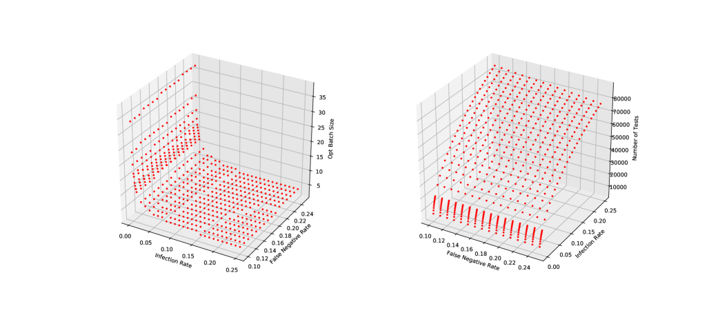
Figure 1: Optimal batch size (left) and required number of batches (right) for the first round of batch tests. False positive rate: $.01$, population size: 100,000.

Figure 1 displays the optimal batch size and the required number of batches for a population of size 100,000 as the infection rate ranges from .001 to .25 for the first round, and the false negative rate ranges from .1 to .25. The false positive rate is fixed at $.01$. Table 1 displays the optimal batch sizes for different infection rates (a) when no testing errors are assumed and (b) when the false negative rate is 15% and the false positive rate is 1%.

Table 1: Optimal batch size (a) when there are no testing errors, and (b) when the false negative rate is .15, false positive rate is .01 for individual tests.

Infection rate	.001	.002	.003	.004	.005	.006	.007	.008	.009	.01	.02	.03
(a) without error	32	23	19	16	15	13	12	12	11	11	8	6
(b) with error	35	25	21	18	16	15	14	13	12	12	8	7
Infection rate	.04	.05	.06	.07	.08	.09 to .12		.13 to .17		.18 to .25
(a) without error	6	5	5	4	4	4		3		3
(b) with error	6	6	5	5	5	4		4		3

2.3 Sensitivity and specificity of a batch test

Let us consider one-step batch testing. If a batch is tested negative, then we conclude that all samples in the batch are negative. If a batch is tested positive, then each sample in the batch needs to be tested individually. Let the binomial random variable $X$ denote the number of positive cases in a batch of size $n$ with an infection rate of $p$. We continue to denote $\alpha$ as the probability of a type I error and $\beta$ as the probability of a type II error for an individual test. Table 2 displays the probabilities for the confusion matrix.

Table 2: Probability in each cell of the confusion matrix for single batch testing.

		True condition
		No samples are infected	At least one sample is infected
Test	$-$	(a) $(1-\alpha)P(X=0)$	(b) $\beta P(X>0)$
Result	$+$	(c) $\alpha P(X=0)$	(d) $(1-\beta)P(X>0)$

2.3.1 Sensitivity

The probability that at least one sample is infected in each batch is $P(X>0)$ which is the sum of the probabilities in cells (b) and (d). In cell (b), it can be deduced that all the samples are negative, and no more tests are given. In cell (d), each sample gets an individual test, and the probability of false negative here is $\beta(1-\beta)P(X>0)$. Thus, the false negative rate is

$$\frac{\beta P(X>0)+\beta(1-\beta)P(X>0)}{P(X>0)}=\beta+\beta(1-\beta)=\beta(2-\beta).$$

For example, if $\beta=.15$, then the false negative rate of batch testing is $.15(2-.15)=.2775$, and thus the sensitivity is .7225. For $\beta=$ .1, .2 and .25, the sensitivity of batch testing is .81, .64 and .5625, respectively. Note that the sensitivity of a batch test depends on neither the infection rate nor the batch size. The above result is supported by our simulation given in Section 3. It confirms that the sensitivity is decreased by conventional batch testing. In contrast, our multi-step batch testing method has a significantly higher sensitivity than conventional individual tests as well as single batch testing as shown in Section 2.5.

2.3.2 Specificity

The false positive error occurs in cells (c) and possibly in (d) in Table 2, and all the samples in these cells go through individual tests. In cell (c), the probability that a sample is incorrectly tested positive in the individual tests is

$$\alpha^{2}P(X=0)=\alpha^{2}(1-p)^{n}.$$ (10)

In cell (d), the expected infection rate in each batch is $p/P(X>0)$. The probability that an uninfected sample is incorrectly tested positive in the individual tests in this cell is

$$(1-\beta)P(X>0)\alpha\left[1-\frac{p}{P(X>0)}\right]=\alpha(1-\beta)[P(X>0)-p]=\alpha(1-\beta)\left[1-(1-p)^{n}-p\right].$$ (11)

The sum of (10) and (11) is

$$\alpha^{2}(1-p)^{n}+\alpha(1-\beta)\left[1-p-(1-p)^{n}\right]=\alpha(1-\beta)(1-p)+\alpha(\alpha+\beta-1)(1-p)^{n}.$$

Therefore, the false positive rate of batch testing is

$$\mbox{Fp}\equiv\frac{\alpha(1-\beta)(1-p)+\alpha(\alpha+\beta-1)(1-p)^{n}}{1-p}=\alpha(1-\beta)+\alpha(\alpha+\beta-1)(1-p)^{n-1}$$

and the specificity of batch testing is

$$1-\mbox{Fp}=(1-\alpha+\alpha\beta)+\alpha(1-\alpha-\beta)(1-p)^{n-1}.$$ (12)

Unlike the sensitivity of batch testing, the batch size, infection rate, probability of a type I error, and probability of a type II error contribute to (12). For $\alpha=$.01 & .03, and $\beta=$.1, 15, .2 & .25, the specificity of batch testing (12) using a fixed batch size of 10, and using the optimal batch size is given in Table 3. The specificity is substantially improved by batch testing. These results closely match with our simulation results given in Section 3.

Table 3: Specificity for single batch testing with fixed batch size of 10 and optimal batch size for the false positive rate of .01, .03, and the false negative rate of .1, .15, .2, .25 for individual tests.

$\alpha$	$\beta$		Infection rate	.001	.01	.03	.05	.10
		Batch size 10	Specificity	.9998	.9991	.9978	.9966	.9944
	.1	Optimal	Batch size	34	11	7	5	4
		batch size	Specificity	.9996	.9990	.9984	.9982	.9975
		Batch size 10	Specificity	.9998	.9992	.9979	.9968	.9948
	.15	Optimal	Batch size	35	12	7	6	4
.01		batch size	Specificity	.9996	.9990	.9985	.9980	.9976
		Batch size 10	Specificity	.9998	.9992	.9980	.9970	.9951
	.2	Optimal	Batch size	36	12	7	6	4
		batch size	Specificity	.9996	.9991	.9986	.9981	.9978
		Batch size 10	Specificity	.9998	.9993	.9981	.9972	.9954
	.25	Optimal	Batch size	37	12	7	6	5
		batch size	Specificity	.9996	.9991	.9987	.9982	.9974
		Batch size 10	Specificity	.9989	.9968	.9928	.9895	.9831
	.1	Optimal	Batch size	34	11	7	5	4
		batch size	Specificity	.9983	.9966	.9947	.9943	.9920
		Batch size 10	Specificity	.9989	.9970	.9932	.9900	.9840
	.15	Optimal	Batch size	36	12	7	6	4
.03		batch size	Specificity	.9983	.9965	.9950	.9935	.9924
		Batch size 10	Specificity	.9989	.9971	.9936	.9906	.9849
	.2	Optimal	Batch size	37	12	7	6	4
		batch size	Specificity	.9983	.9967	.9952	.9939	.9928
		Batch size 10	Specificity	.9989	.9972	.9939	.9911	.9859
	.25	Optimal	Batch size	38	13	8	6	5
		batch size	Specificity	.9983	.9966	.9950	.9942	.9917

2.4 PPV and NPV

Let us define $E$ as the event that an individual is infected by the virus, and $B$ as the event that an individual got a positive test result. Then by the Bayes’ rule, PPV (positive predictive value: an individual is infected given a positive test result) is

$$P(E|B)=\frac{P(B|E)P(E)}{P(B|E)P(E)+P\left(B|E^{C}\right)P\left(E^{C}\right)}$$

and NPV (negative predictive value: an individual is not infected given a negative test result) is

$$P\left(E^{C}|B^{C}\right)=\frac{P\left(B^{C}|E^{C}\right)P\left(E^{C}\right)}{P\left(B^{C}|E^{C}\right)P\left(E^{C}\right)+P\left(B^{C}|E\right)P(E)}.$$

For example, if the infection rate in the population is 1%, sensitivity is 85%, and specificity is 99%, then $P(E)=0.01,~{}P(B|E)=0.85$ and $P\left(B^{C}|E^{C}\right)=0.99$. Therefore, the PPV is .4620 and the NPV is .9985. If the infection rate is .1%, then the PPV is .0078 and the NPV is .9998. For the infection rates $p\in[.001,.2]$, sensitivity within the range of [.75, .90] and the specificity of .99, Table 4 illustrates PPV and NPV. Figure 2 displays the PPV (above) and NPV (below). By batch testing, the PPV is significantly improved. If we denote $S_{e}(B)$ as the sensitivity and $S_{p}(B)$ as the specificity of single-step batch testing, the PPV and NPV of single-step batch testing are given as

$$\mbox{PPV}(B) = \frac{(1-p)[1-S_{p}(B)]}{(1-p)[1-S_{p}(T)]+pS_{e}(B)}$$

$$\mbox{NPV}(B) = \frac{p[1-S_{e}(B)]}{p[1-S_{e}(T)]+(1-p)S_{p}(B)}$$

respectively (Fletcher et al., 1988; Litvak et al., 1994; Kim et al., 2007). For the infection rate of .1%, PPV$(B)$ is .8049 and NPV$(B)$ is .9997. For the infection rate of 1%, PPV$(B)$ is .8983 and NPV$(B)$ is .9972. These numbers are obtained by substituting the values from Section 2.3.1 and Section 2.3.2 when a fixed batch size of 10 is used. The PPV is further improved by our multi-step batch testing procedure (see Section 3).

Table 4: PPV and NPV.

		Sensitivity(1)
$p^{(2)}$		.75	.77	.79	.81	.83	.85	.87	.89	.90
.001	PPV	.0070	.0072	.0073	.0075	.0077	.0078	.0080	.0082	.0083
	NPV	.9997	.9998	.9998	.9998	.9998	.9998	.9999	.9999	.9999
.002	PPV	.1307	.1337	.1367	.1397	.1426	.1455	.1485	.1514	.1528
	NPV	.9995	.9995	.9996	.9996	.9997	.9997	.9997	.9998	.9998
.004	PPV	.2315	.2362	.2409	.2455	.2500	.2545	.2589	.2633	.2655
	NPV	.9990	.9991	.9991	.9992	.9993	.9994	.9995	.9996	.9996
.006	PPV	.3116	.3173	.3229	.3284	.3338	.3391	.3443	.3495	.3520
	NPV	.9985	.9986	.9987	.9988	.9990	.9991	.9992	.9993	.9994
.008	PPV	.3769	.3831	.3892	.3951	.4010	.4067	.4123	.4178	.4206
	NPV	.9980	.9981	.9983	.9985	.9986	.9988	.9989	.9991	.9992
.01	PPV	.4310	.4375	.4438	.5500	.4560	.4620	.4677	.4734	.4762
	NPV	.9975	.9977	.9979	.9981	.9983	.9985	.9987	.9989	.9990
.02	PPV	.6048	.6111	.6172	.6231	.6288	.6343	.6397	.6449	.6475
	NPV	.9949	.9953	.9957	.9961	.9965	.9969	.9973	.9977	.9979
.03	PPV	.6988	.7043	.7096	.7147	.7197	.7244	.7291	.7335	.7357
	NPV	.9923	.9929	.9935	.9941	.9947	.9953	.9960	.9966	.9969
.05	PPV	.7978	.8021	.8061	.8100	.8137	.8173	.8208	.8241	.8257
	NPV	.9869	.9879	.9890	.9900	.9910	.9921	.9931	.9942	.9947
.08	PPV	.8671	.8701	.8729	.8757	.8783	.8808	.8832	.8856	.8867
	NPV	.9785	.9802	.9819	.9836	.9853	.9870	.9887	.9904	.9913
.10	PPV	.8929	.8953	.8978	.9000	.9022	.9043	.9063	.9082	.9091
	NPV	.9727	.9748	.9770	.9791	.9813	.9834	.9856	.9878	.9889
.15	PPV	.9298	.9315	.9331	.9346	.9361	.9375	.9388	.9401	.9408
	NPV	.9573	.9606	.0639	.9672	.9706	.9740	.9774	.9808	.9825
.20	PPV	.9494	.9506	.9518	.9529	.9540	.9551	.9560	.9570	.9574
	NPV	.9406	.9451	.9496	.9542	.9588	.9635	.9682	.9730	.9754

⁽¹⁾Specificity is .99   ⁽²⁾Infection rate

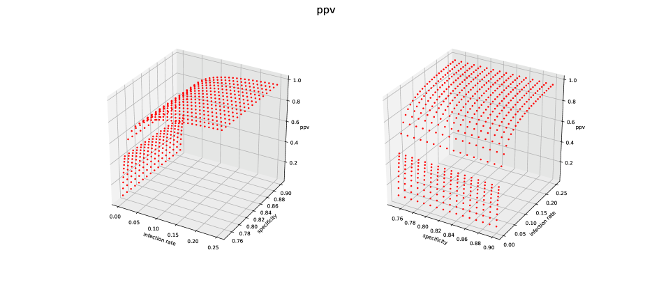
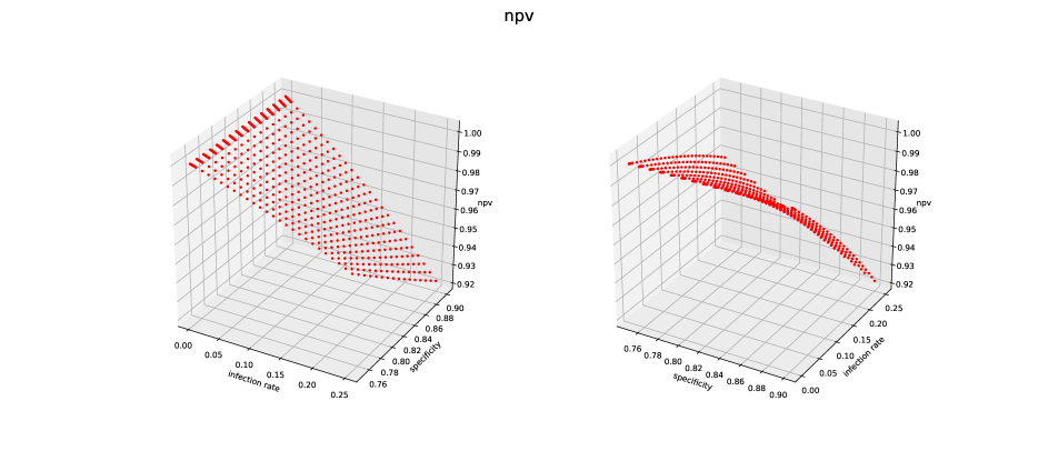
Figure 2: PPV (above) and NPV (below).

2.5 Multi-step batch testing procedure

More than 3 batch negatives may not be necessary in the procedure because the infection rate substantially decreases in later rounds. Figure 3 illustrates the proposed batch testing procedure. We will further investigate the optimal number of batch tests and the stopping rule in this study. For batch negatives, the batch size increases substantially with most of the subjects remaining in the next round because the infection rate decreases. For batch positives, the subpopulation size substantially decreases in the next round. In this group, not all the samples in the batch are infected, so we may find a sample without infection in the next round of batch tests. This way, the number of required tests to cover the whole population decreases significantly, and it is possible to identify all positive carriers in the population.

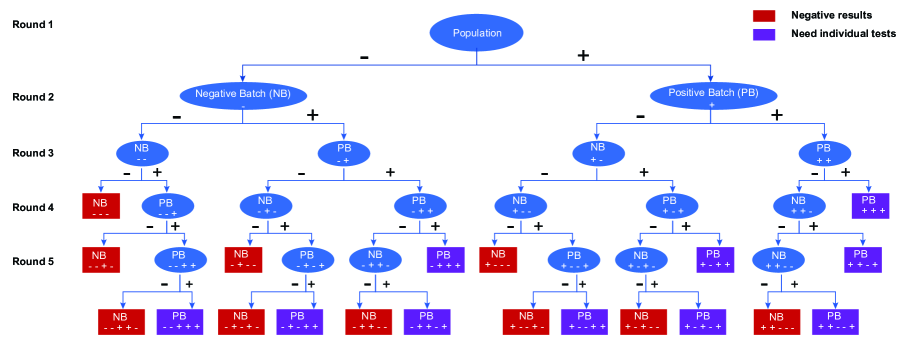
Figure 3: Proposed multi-step batch testing procedure. The oval nodes indicate intermediate nodes and the rectangular nodes indicate terminal nodes.

We assume 15% false negative rate and 1% false positive rate of an individual for a population of size 100,000 in this section. Table 5 shows the change in the infection rate and corresponding optimal batch size throughout the process shown in Figure 3 for a population with infection rates of .1% and 1%. In the first round, the optimal batch size is 35 resulting in 2,858 batch tests when the infection rate is .1%, and the optimal batch size is 12 resulting in 8,334 batch tests when the infection rate is 1%. Note that the number of batch tests for the first round can be slightly different from this estimation due to the trial for estimating the infection rate with (4) using a small subset of the population with an initial guess of the batch size. The subsequent rounds do not require this trial because the infection rates of subpopulations can be estimated as (8) using the values obtained in the previous round. For the $i$th round, the number of batch tests can be obtained by ceiling$(N_{i}/n_{i})$. We count only the bold-faced numbers starting the first round because the rest are duplicates. In each of Round 2 and Round 3, the bold-faced subpopulation sizes ($N_{i}$) add up to 100,000 if we ignore the rounding error. In Round 4, the bold-faced subpopulation sizes plus $N$ in the final column for already finished ($---$ and $+++$) rows add up to 100,000. The calculation is similar for Round 5. The final two columns show the infection rate and resulting subpopulation size in each of the terminal nodes (rectangular frames) in Figure 3. For each infection rate, since the individuals in an upper half of the last column got 3 batch negatives, they do not need individual tests. A lower half of the last column needs individual tests because they got 3 batch positives. Thus, the total number of individual tests is the sum of these 10 numbers. The total number of tests can be obtained by adding the number of batch tests in Round 1, the number of batch tests obtained from the bold-faced numbers in the subsequent rounds, and the number of individual tests.

Table 5: Batch test procedure^∗: population size 100,000, false negative rate 15% & false positive rate 1% for individual tests, infection rates .1% and 1%.

Infection rate$=.1\%$. The first round requires 2858 tests with batch size 35.
	Round 2			Round 3			Round 4			Round 5			Final
Tests	$p_{2}^{(1)}$	$N_{2}^{(2)}$	$n_{2}^{(3)}$	$p_{3}$	$N_{3}$	$n_{3}$	$p_{4}$	$N_{4}$	$n_{4}$	$p_{5}$	$N_{5}$	$n_{5}$	$p$	$N$
$---$	2e-4	96109	88	2e-5	94047	224							4e-6	92684
$--+-$	2e-4	96109	88	2e-5	94047	224	.001	1363	30				2e-4	1302
$-+--$	2e-4	96109	88	.006	2062	15	.001	1888	35				2e-4	1814
$+---$	.022	3891	8	.004	3322	18	6e-4	3102	45				1e-4	3000
$--++-$	2e-4	96109	88	2e-5	94047	224	.001	1363	30	.027	61	7	.005	51
$-+-+-$	2e-4	96109	88	.006	2062	15	.001	1888	35	.022	74	8	.004	63
$-++--$	2e-4	96109	88	.006	2062	15	.062	175	5	.012	133	10	.002	118
$+--+-$	.022	3891	8	.004	3322	18	6e-4	3102	45	.016	102	9	.003	90
$+-+--$	.022	3891	8	.004	3322	18	.049	220	6	.010	169	12	.002	152
$++---$	.022	3891	8	.13	568	4	.03	362	7	.005	300	15	.001	278
$+++$	.022	3891	8	.13	568	4							.30	206
$++-+$	.022	3891	8	.13	568	4	.03	362	7				.15	62
$+-++$	.022	3891	8	.004	3322	18	.049	220	6				.18	51
$-+++$	2e-4	96109	88	.006	2062	15	.062	175	5				.22	42
$++--+$	.022	3891	8	.13	568	4	.03	362	7	.005	300	15	.06	23
$+-+-+$	.022	3891	8	.004	3322	18	.049	220	6	.010	169	12	.08	17
$+--++$	.022	3891	8	.004	3322	18	6e-4	3102	45	.016	102	9	.11	13
$-++-+$	2e-4	96109	88	.006	2062	15	.062	175	5	.012	133	10	.10	14
$-+-++$	2e-4	96109	88	.006	2062	15	.001	1888	35	.022	74	8	.13	11
$--+++$	2e-4	96109	88	2e-5	94047	224	.001	1363	30	.027	61	7	.15	9

Infection rate$=1\%$. The first round requires 8335 tests with batch size 12.
	Round 2			Round 3			Round 4			Round 5			Final
Tests	$p_{2}$	$N_{2}$	$n_{2}$	$p_{3}$	$N_{3}$	$n_{3}$	$p_{4}$	$N_{4}$	$n_{4}$	$p_{5}$	$N_{5}$	$n_{5}$	$p$	$N$
$---$	.002	89456	27	3e-4	85233	68							4e-5	83107
$--+-$	.002	89456	27	3e-4	85233	68	.009	2126	12				.0015	1921
$-+--$	.002	89456	27	.03	4223	7	.006	3496	15				.0009	3229
$+---$	.08	10544	5	.017	7399	9	.003	6425	21				.0005	6033
$--++-$	.002	89456	27	3e-4	85233	68	.009	2126	12	.079	205	5	.017	144
$-+-+-$	.002	89456	27	.03	4223	7	.006	3496	15	.061	267	5	.012	204
$-++--$	.002	89456	27	.03	4223	7	.15	727	4	.038	430	6	.007	351
$+--+-$	.08	10544	5	.017	7399	9	.003	6425	21	.041	392	6	.008	314
$+-+--$	.08	10544	5	.017	7399	9	.11	974	4	.025	657	8	.0044	550
$++---$	.08	10544	5	.23	3144	3	.065	1679	5	.013	1262	10	.0022	1120
$+++$	.08	10544	5	.23	3144	3							.42	1466
$++-+$	.08	10544	5	.23	3144	3	.065	1679	5				.22	417
$+-++$	.08	10544	5	.017	7399	9	.11	974	4				.29	317
$-+++$	.002	89456	27	.03	4223	7	.15	727	4				.31	298
$++--+$	.08	10544	5	.23	3144	3	.065	1679	5	.013	1262	10	.10	142
$+-+-+$	.08	10544	5	.017	7399	9	.11	974	4	.025	657	8	.13	107
$+--++$	.08	10544	5	.017	7399	9	.003	6425	21	.041	392	6	.18	78
$-++-+$	.002	89456	27	.03	4223	7	.15	727	4	.038	430	6	.18	79
$-+-++$	.002	89456	27	.03	4223	7	.006	3496	15	.061	267	5	.22	63
$--+++$	.002	89456	27	3e-4	85233	68	.009	2126	12	.079	205	5	.23	60

⁽¹⁾infection rate   ⁽²⁾subpopulation size   ⁽³⁾batch size

The expected number of tests to identify all positive carriers is 6,144 (5,696 batch tests and 448 individual tests) when the infection rate is .1%, and 22,436 (19,409 batch tests and 3,027 individual tests) when the infection rate is 1%. The sensitivity of this procedure can be obtained from the number of individual tests with the corresponding infection rates given in the last two columns in Table 5. For the infection rate of .1%, the expected number of infected cases among the samples who received individual tests at the end of the procedure is 97.8 out of 448. With the 85% sensitivity for individual tests, the sensitivity of this procedure is 83.1% since $97.8\times.85=83.1$ out of 100. For the infection rate of 1%, the expected number of infected cases among the samples who received individual tests is 975.5 out of 3,027. The sensitivity of this procedure is 82.9% since $975.5\times.85=829$ out of 1,000. To calculate the specificity, for the infection rate of .1%, the expected number of uninfected samples among the samples who received individual tests is 350.2 out of 448. With the 1% type I error rate for individual tests, since $350.2\times.01=3.502$, the specificity of this procedure is $100\left[1-(3.502/99,900)\right]\%=99.996\%$. For the infection rate of 1%, the expected number of uninfected samples among the samples who received individual tests is 2,051.5 out of 3,027. Since $2,051.5\times.01=20.515$, the specificity of this procedure is $100\left[1-(20.515/99,000)\right]\%=99.98\%$. These results closely match with our simulation results given for method (E) in Table 7 of Section 3.

To reduce the false negative rate, we propose to conduct sequential individual tests as follows: We conduct up to 3 tests for the same person sequentially until a positive test occurs. Let us define $E$ as the event that an individual is infected, and $B_{i}$ as the event that an individual got a positive result in the $i$th individual test. Then the probability that a sample is tested positive in the first test is

$$p_{1}\equiv P(B_{1})=P(B_{1}|E)P(E)+P\left(B_{1}|E^{C}\right)P\left(E^{C}\right),$$

the probability that a person is tested negative and then tested positive is

$$p_{2}\equiv P\left(B_{1}^{C}\cap B_{2}\right)=P\left(B_{1}^{C}\cap B_{2}|E\right)P(E)+P\left(B_{1}^{C}\cap B_{2}|E^{C}\right)P\left(E^{C}\right)$$

and a person is tested negative twice is

$$p_{3}\equiv P\left(B_{1}^{C}\cap B_{2}^{C}\right)=1-(p_{1}+p_{2}).$$

Thus, the expected number of the individual tests for each person is

$$p_{1}+2p_{2}+3p_{3}.$$ (13)

We can obtain the expected total number of sequential individual tests by substituting the infection rate and the subpopulation size in each of the bottom 10 rows of the last two columns in Table 5. For the infection rate of .1%, the expected number of sequential individual tests in (13) is 1,155, and the expected number of tests for the whole procedure becomes 6,851. For the infection rate of 1%, the expected number of sequential individual tests is 7,236, and the expected number of tests for the whole procedure is 26,645. The sensitivity of this method can be obtained by multiplying $1-\beta^{3}=1-.15^{3}=.996625$ to the expected number of infected cases in the sequential individual testing. Recall that the expected number of infected cases among the samples who received individual tests was 97.8 and 975.5 for infection rates .1% and 1%, respectively. For the infection rate of .1%, the sensitivity of this method is 97.5% since $97.8\times.996625=97.5$ out of 100. For the infection rate of 1%, the sensitivity of this method is 97.2% since $975.5\times.996625=972$ out of 1,000. To calculate the specificity of this method, the probability that an uninfected sample is concluded as positive in the sequential testing is $1-(1-\alpha)^{3}=1-.99^{3}=.029701$. For the infection rate of .1%, since $350.2\times.029701=10.4$, the specificity of this method is $100\left[1-(10.4/99,900)\right]\%=99.99\%$. For the infection rate of 1%, since $2,051.5\times.029701=60.931$, the specificity of this method is $100\left[1-(60.931/99,000)\right]\%=99.94\%$. These results closely match with our simulation results given for method (F) in Table 7 of Section 3.

Table 6: Possible cases of the proposed batch test procedure with false negative rates.

	Conclusion to the final batch:							Individual tests
	no infection							for the final batch
		Batch test round					False		Batch test round					False
#tests	Case	1	2	3	4	5	negative rate	Case	1	2	3	4	5	negative rate
3	(1)	$-$	$-$	$-$			$\beta^{3}$	(11)	$+$	$+$	$+$			$(1-\beta)^{3}\beta^{3}$
4	(2)	$-$	$-$	$+$	$-$		$(1-\beta)\beta^{3}$	(12)	$+$	$+$	$-$	$+$		$(1-\beta)^{3}\beta^{4}$
4	(3)	$-$	$+$	$-$	$-$		$(1-\beta)\beta^{3}$	(13)	$+$	$-$	$+$	$+$		$(1-\beta)^{3}\beta^{4}$
4	(4)	$+$	$-$	$-$	$-$		$(1-\beta)\beta^{3}$	(14)	$-$	$+$	$+$	$+$		$(1-\beta)^{3}\beta^{4}$
5	(5)	$-$	$-$	$+$	$+$	$-$	$(1-\beta)^{2}\beta^{3}$	(15)	$+$	$+$	$-$	$-$	$+$	$(1-\beta)^{3}\beta^{5}$
5	(6)	$-$	$+$	$-$	$+$	$-$	$(1-\beta)^{2}\beta^{3}$	(16)	$+$	$-$	$+$	$-$	$+$	$(1-\beta)^{3}\beta^{5}$
5	(7)	$-$	$+$	$+$	$-$	$-$	$(1-\beta)^{2}\beta^{3}$	(17)	$+$	$-$	$-$	$+$	$+$	$(1-\beta)^{3}\beta^{5}$
5	(8)	$+$	$-$	$-$	$+$	$-$	$(1-\beta)^{2}\beta^{3}$	(18)	$-$	$+$	$+$	$-$	$+$	$(1-\beta)^{3}\beta^{5}$
5	(9)	$+$	$-$	$+$	$-$	$-$	$(1-\beta)^{2}\beta^{3}$	(19)	$-$	$+$	$-$	$+$	$+$	$(1-\beta)^{3}\beta^{5}$
5	(10)	$+$	$+$	$-$	$-$	$-$	$(1-\beta)^{2}\beta^{3}$	(20)	$-$	$-$	$+$	$+$	$+$	$(1-\beta)^{3}\beta^{5}$

To further illustrate how the false negative rate is reduced by this procedure, Table 6 lists all possible cases shown in Table 5 with the false negative rate in each case. Among the 20 possible cases of batch testing, the first 10 cases result in 3 batch negatives, and the second 10 cases result in 3 batch positives. If a sample is in one of the first 10 cases, then it will be deduced as uninfected, and if it is in one of the second 10 cases, then it requires up to 3 sequential individual tests. The false negative rate is $\beta^{3}=.003375$ for Case (1) because it has 3 batch negatives, $(1-\beta)\beta^{3}=.00287$ for Cases (2) through (4) because it has 3 batch negatives and 1 batch positive, and $(1-\beta)^{2}\beta^{3}=.00244$ for Cases (5) through (10) because it has 3 batch negatives and 2 batch positives. Since false negative occurs when a sample gets negative in all three individual tests sequentially, $\beta^{3}$ is multiplied by the rates given in Table 6 to the second 10 cases. The false negative rate is $(1-\beta)^{3}\beta^{3}=.00207$ for Case (11), $(1-\beta)^{3}\beta^{4}=.00031$ for Cases (12) through (14), and $(1-\beta)^{3}\beta^{5}=.000047$ for Cases (15) through (20). An estimation of the false negative rate of the proposed batch testing procedure can be obtained by multiplying the false negative rate with the subpopulation size given in the last column of Table 5 in each case and divide the sum of these 20 numbers by the population size of 100,000. The estimated false negative rate is 3.33% when the infection rate is .1%, and 3.25% when the infection rate is 1%. These results yield the sensitivity of 96.67% and 96.75%, respectively. These estimates of the sensitivity are slightly lower and the estimates by combining groups of 10 cases in the previous paragraph (97.5% and 97.2%, respectively) are slightly higher than the simulation results for method (F) in Table 7 given in Section 3, but they are within one standard deviation (1.65% for infection rate .1% and .57% for infection rate 1%).

3 Simulation Studies

We conducted a Monte Carlo simulation study to evaluate the efficiency and efficacy of the proposed batch testing procedure. In this simulation, we assume that the sensitivity and specificity of individual tests are 85% and 99%, respectively. A population of 100,000 people is randomly generated 100 times. The infection rates of .1%, 1%, 3%, 5% and 10% are chosen. Table 7 compares our methods with conventional individual tests, single batch tests, and matrix pool tests using various accuracy measures. We compare the accuracy measures for (A) conventional individual tests, (B) one-step batch testing with a fixed batch size of 10, (C) one-step batch testing with optimal batch sizes, with up to 3 sequential individual tests for each of the positive batches, (D) parallel $12\times 12$ matrix pool testing (to cover the whole population, 694 $12\times 12$ matrices and one $8\times 8$ matrix are used); up to 3 sequential individual tests for all the positive intersections. Since a single matrix testing gives very low sensitivity, we report results from three parallel matrix pool tests. (E) proposed multi-step batch tests ending with three batch negatives or three batch positives, with an individual test given to three batch positives, (F) multi-step batch tests given in (E), with up to 3 sequential individual tests for three batch positives. For (C), (E) and (F), the optimal batch sizes estimated in Section 2.5 are used in the subpopulations in each step. For each of the infection rates, the overall accuracy, sensitivity, specificity, PPV and NPV are calculated, and the required number of tests to cover the whole population is calculated from this simulation, and the values are averaged over the 100 repetitions. The fixed batch size of 10 given in (B) has been used in South Korea for high-risk facilities. For multi-step batch testing, individual tests are conducted to the subpopulation if the infection rate exceeds 30% in any step as mentioned in Section 1. Another set of simulation results for sensitivity of 75% and specificity of 97% is given in the Appendix. The comparison between our methods and the conventional individual tests, single batch testing, or matrix pool tests gives a similar pattern to the one given in this section.

Table 7: Simulation results: 100 repetitions, population size 100,000, sensitivity 85% & specificity 99% for individual tests; mean with standard deviation in parentheses.

$p^{(1)}$		.001	.01	.03	.05	.10
(A)a	Acc.(2)	.9899 (.0003)	.9886 (.0003)	.9859 (.0004)	.9831 (.0004)	.9760 (.0004)
Indiv	Sens.(3)	.8525 (.0356)	.8491 (.0105)	.8500 (.0067)	.8509 (.0051)	.8497 (.0030)
Tests	Spec.(4)	.9900 (.0003)	.9900 (.0003)	.9901 (.0003)	.9900 (.0003)	.9900 (.0003)
	PPV	.0799 (.0088)	.4621 (.0107)	.7251 (.0075)	.8176 (.0054)	.9041 (.0031)
	NPV	.9998 (.0000)	.9985 (.0001)	.9954 (.0002)	.9921 (.0003)	.9834 (.0004)
	#Tests(5)	100000 (0)	100000 (0)	100000 (0)	100000 (0)	100000 (0)
(B)b	Acc.	.9995 (.0001)	.9964 (.0002)	.9897 (.0003)	.9831 (.0005)	.9675 (.0006)
Single	Sens.	.7261 (.0413)	.7213 (.0163)	.7241 (.0093)	.7219 (.0075)	.7221 (.0052)
Batch	Spec.	.9998 (.0000)	.9992 (.0001)	.9979 (.0002)	.9968 (.0002)	.9948 (.0003)
Tests	PPV	.8074 (.0449)	.8998 (.0101)	.9136 (.0057)	.9227 (.0039)	.9389 (.0028)
Fixed	NPV	.9997 (.0001)	.9972 (.0002)	.9915 (.0003)	.9855 (.0004)	.9699 (.0006)
Size 10	#Tests	11841 (133)	18981 (259)	33108 (438)	44693 (500)	65671 (519)
(C)c	Acc.	.9987 (.0001)	.9956 (.0002)	.9911 (.0003)	.9868 (.0004)	.9784 (.0005)
Single	Sens.	.8420 (.0384)	.8453 (.0128)	.8464 (.0074)	.8470 (.0059)	.8466 (.0042)
Batch	Spec.	.9989 (.0001)	.9971 (.0002)	.9956 (.0002)	.9941 (.0002)	.9930 (.0003)
Variable	PPV	.4308 (.0268)	.7460 (.0124)	.8548 (.0067)	.8835 (.0040)	.9303 (.0027)
Sizes	NPV	.9998 (.0000)	.9984 (.0001)	.9952 (.0002)	.9920 (.0003)	.9832 (.0005)
Seq Indiv	#Tests	14393 (1128)	37889 (824)	60567 (817)	77952 (793)	98341 (739)
Tests	B+Ind	2858+11535	8334+29555	14286+46281	16667+61285	25000+73341
(D)d	Acc.	.9999 (.0000)	.9994 (.0001)	.9970 (.0002)	.9939 (.0003)	.9863 (.0005)
Parallel	Sens.	.9907 (.0106)	.9897 (.0048)	.9905 (.0031)	.9901 (.0031)	.9905 (.0029)
$12\times 12$	Spec.	.9999 (.0000)	.9995 (.0001)	.9972 (.0002)	.9941 (.0003)	.9858 (.0005)
Matrix	PPV	.9402 (.0332)	.9511 (.0077)	.9168 (.0053)	.8980 (.0041)	.8857 (.0032)
Tests	NPV	1.000 (.0000)	.9999 (.0000)	.9997 (.0001)	.9995 (.0002)	.9989 (.0003)
Seq Indiv	#Tests	50727 (342)	56201 (550)	80478 (971)	112177 (1458)	190263 (1951)
Test	B+Ind	49968+759	49968+6233	49968+30510	49968+62209	49968+140295
(E)e	Acc.	.9998 (.0000)	.9981 (.0001)	.9941 (.0003)	.9905 (.0003)	.9814 (.0005)
Multi-step	Sens.	.8305 (.0337)	.8281 (.0120)	.8306 (.0066)	.8291 (.0053)	.8296 (.0041)
Batch	Spec.	1.000 (.0000)	.9998 (.0001)	.9992 (.0001)	.9990 (.0001)	.9983 (.0001)
Variable	PPV	.9503 (.0241)	.9722 (.0058)	.9693 (.0037)	.9776 (.0021)	.9815 (.0014)
Sizes	NPV	.9998 (.0000)	.9983 (.0001)	.9948 (.0002)	.9911 (.0003)	.9814 (.0005)
1 indiv	#Tests	6221 (159)	22840 (280)	42561 (316)	56089 (377)	84012 (375)
Test	B+Ind	5705+516	19439+3401	31830+10731	41554+14535	58622+25390
(F)f Multi-	Acc.	.9998 (.0000)	.9990 (.0001)	.9969 (.0002)	.9958 (.0002)	.9926 (.0003)
step Batch	Sens.	.9689 (.0165)	.9700 (.0057)	.9730 (.0033)	.9723 (.0025)	.9725 (.0017)
Variable	Spec.	.9999 (.0000)	.9993 (.0001)	.9976 (.0002)	.9970 (.0002)	.9949 (.0002)
Sizes	PPV	.8852 (.0290)	.9307 (.0085)	.9259 (.0044)	.9446 (.0028)	.9547 (.0018)
Seq Indiv	NPV	1.000 (.0000)	.9997 (.0001)	.9992 (.0001)	.9985 (.0001)	.9969 (.0002)
Tests for	#Tests	7053 (259)	27809 (404)	58428 (609)	75908 (600)	116341 (718)
3 $+$’s	B+Ind	5704+1349	19436+8373	31809+26619	41530+34378	58611+57730

^aConventional individual tests
^bOne-step batch tests with a fixed batch size of 10, individual tests for positive batches
^cOne-step batch tests with variable batch sizes with up to 3 sequential individual tests for positive batches
^dThree parallel matrix pool tests; up to 3 sequential individual tests to all positive intersections
^eMulti-step batch tests with variable optimal batch sizes; an individual test for 3 batch positives
^fMulti-step batch tests; up to 3 sequential individual tests for 3 batch positives
⁽¹⁾infection rate  ⁽²⁾overall accuracy  ⁽³⁾sensitivity  ⁽⁴⁾specificity  ⁽⁵⁾Number of required tests
⁽⁶⁾number of batch tests $+$ number of individual tests

For the matrix pool testing, we also simulated conventional one-step matrix pool test with an individual test to the positive intersection, but the sensitivity was less than 62% for all the infection rates. For one-step matrix pool tests with up to 3 sequential tests to each of the positive intersection, the sensitivity was around 72%. For 3 parallel matrix pool tests with an individual test to all positive intersections, the sensitivity was around 84%. To achieve high performance for the comparison, we report simulation results for 3 parallel matrix pool tests with up to 3 sequential individual tests to all positive intersections in (D). Although not reported in this paper, single-step batch testing with variable batch sizes also was conducted. The accuracy measures were very close to those of the fixed batch size in (B). However, the batch tests with variable batch sizes require fewer tests.

Note that the number of required tests in the proposed method (F) is close to the estimated number derived in Section 2.5. The sensitivity is reduced in the one-step batch tests (given in (B)) to approximately 72% from conventional individual tests. This is because if a batch is tested negative, then all the samples in the batch are considered uninfected, and no further tests are given. The results are in line with the sensitivity of 72.25% for one-step batch testing obtained in Section 2.3.1. Method (C) substantially improved the sensitivity to almost the same level as the sensitivity of conventional individual tests. The sensitivity of method (E) is around 83%, and it is improved by method (F) to approximately 97%. These results show that both the multi-step batch testing and sequential individual tests significantly improve the sensitivity. These are in line with the numbers obtained from the model in Section 2.5. This improvement is achieved because sequential individual tests are given to small target subpopulations obtained by our test procedure. Although not included in Table 7, we also conducted a simulation of multi-step batch testing with a fixed batch size of 10 followed by up to 3 sequential individual tests. The sensitivity of this method was almost identical to that of method (F) because the sensitivity does not depend on the batch size. However, method (F) requires much fewer tests by using the optimal batch sizes (7,053 for method (F) vs. 32,118 for a fixed batch size for infection rate .1%, and 27,809 for method (F) vs. 46,416 for a fixed batch size for infection rate 1%). The sensitivity of method (D) is around 99%. However, the number of tests for matrix pool testing is 50,727 for the infection rate of .1% and 56,201 for the infection rate of 1%. Although not included in the simulation table, we also simulated 3 parallel batch testing with a fixed batch size of 10. The sensitivity of the method was near 85%, and the number of tests to cover the whole population was slightly over 30,000 which is larger than that of method (F) for infection rates of .1% or 1%, but fewer for the infection rates higher than 1%. The sensitivity of this parallel batch testing was much lower than that of method (F).

As mentioned in Section 2.3.2, the specificity is significantly improved by batch testing from conventional individual testing. The specificity of single batch testing obtained in this simulation closely matches with the expected value given in (12). See also Table 3. Although the specificity of the batch tests decreases as the infection rate increases, the one-dimensional batch tests (B, C, E and F) have much higher specificity than the baseline of 99% for all infection rates in Table 7. However, the specificity of the matrix pool tests decreases fast as the infection rate increases and it becomes lower than 99% for the infection rate of 10%.

The improvement of the PPV by our procedure is remarkable. As discussed in Section 2.4 (also shown in (A) of Table 7), the PPV of an individual test is 8% and 46% when the infection rates are .1% and 1%, respectively. According to our simulation, single-step batch testing in (B) improves this to 81% and 90%, respectively, and it is further improved by multi-step batch testing given in (E) to 95% and 97%, respectively. The PPV is decreased by sequential individual tests. It is 43% and 75%, respectively in (C). However, it is improved to 88.5% and 93%, respectively in (F) by multi-step batch testing. The PPV is 94% and 95%, respectively for the matrix pool tests in (D).

The overall number of batch tests from the simulation is close to the estimated number from our model given in Section 2.2. For .1% infection rate, the number of multi-step batch tests in the simulation (methods (E) and (F)) is around 5,700 and the estimated number is 5,696. For 1% infection rate, the number is around 19,440 from the simulation and 19,409 from our estimation. However, the simulated number of individual tests for samples with 3 batch positives is slightly higher than the predicted value. This is likely due to randomness. This discrepancy does not significantly impact the overall number of tests because the size of the subpopulation requiring individual tests is very small (approximately 0.5% for .1% infection rate, and around 3% for 1% infection rate) compared to the whole population. For .1% infection rate, for example, 516 people received individual tests in the simulation (given in (E)), whereas the model estimates that 448 people need individual tests. This means approximately 99.5% of the population do not require individual tests. The model estimate of this value is 99.552% ($100,000-448$ out of $100,000$), and the simulated value is 99.484% ($100,000-516$ out of $100,000$).

Note that the overall accuracy is mostly affected by specificity because the infection rates are low. We can incorporate geographic and demographic information for more realistic calculation.

4 Discussion

The COVID-19 pandemic changed our lifestyle, seriously impacted the global economy, and took many precious lives. To get back to normalcy, we need a rapid testing of the virus for all the residents of each community. Unlike other coronavirus outbreaks we experienced in the past, the disease rapidly spreads silently by asymptomatic carriers. Since only patients with symptoms have been getting tests, it is a challenging task to identify asymptomatic COVID-19 carriers. In most countries including the US, some patients with symptoms could not get tests due to the limited testing capacity. To conduct testing a broader population more efficiently, batch testing methods have been introduced.

The South Korean Center for Disease Control & Prevention used a single-step batch testing for long-term care facilities with a fixed batch size of 10 for the entire staff and patients. As seen in our simulation studies, batch testing increases the false negative rate, although this approach can monitor high-risk groups without symptoms by reducing the number of tests needed to cover the entire community. In this paper, we proposed a multi-step batch testing procedure to substantially decrease the false negative rate using a small number of test kits to completely test a large population. The improvement of PPV from individual testing is also remarkable, and thus our multi-step approach can be trusted for reliable results. Table 5 shows that the proposed batch procedure is effective for a population with a low or moderate infection rate.

Our approach will be useful for the prevention for early stages of future pandemics. Our method is most effective for diseases with infection rates of up to 3%. We do not recommend this approach for highly contagious large populations with infection rates greater than 5%, as the prescribed number of tests becomes very large. Shuren (2020) addressed that conventional batch testing has a higher chance of false negative results because samples are diluted, but it works well when there is a low prevalence of cases. Yelin et al. (2020) found that positive samples can still be well observed in pools in up to 32 samples, and possibly even 64 with additional PCR cycles. However, the detection of positives in a large pool is possible only when viral loads are very high. In future studies, we will investigate the presence of the dilution effect. We will also investigate optimal stopping rules to further improve the efficiency and efficacy of the multi-step batch testing procedure.

References

• Chen, C., Nikolic, J., Gingrich, J. C. and de Jong, P. J. (1992). A two-dimensional YAC pooling strategy for library screening via STS and Alu-PCR methods. Nucleic Acids Research, 25, 2559-63.

• (2020). Group testing with nested pools. https://arxiv.org/abs/2005.13650.

• (1991). Theoretical analysis of library screening using a N-dimensional pooling strategy. Nucleic Acids Research, 19, 6241-6247.

• Kashamuka, M., Atikala, L., Brown, C., Ryder, R. W. and Quinn, T. C. (1990). Successful use of pooled sera to determine HIV-1 seroprevalence in Zaire with development of cost-efficiency models. AIDS, 4, 737-741.

• (2009). Bias, efficiency, and agreement for group-testing regression models. The Journal of Statistical Computation and Simulation, 79, 67-80.

• Tobler, L., Kamel, H., Linnen, J., Shyamala, V., Tomasulo, P. and Kleinman, S. (2005). Screening the blood supply for West Nile virus RNA by nucleic acid amplification testing. New England Journal of Medicine, 353, 460-467.

• (1990). Using group testing to estimate a proportion, and to test the binomial model. Biometrics, 46, 1035-1046.

• (2009). Group testing regression models with fixed and random effects. Biometrics, 65, 1270-1278.

• (2020). Statistical methods for batch screening of input populations by stage and group in COVID-19 nucleic acid testing. medRxiv. doi: 10.1101/2020.04.02.20050914.

• (2011). Nonparametric regression analysis for group testing data. Journal of the American Statistical Association, 106, 640-650.

• (1943). The detection of defective members of large populations. The Annals of Mathematical Statistics, 14, 436-440.

• (2006). Pathogen detection, testing and control in fresh broccoli sprouts. Nutrition Journal, 5, 13.

• (1992). Estimating prevalence by group testing using generalized linear models. Statistics in Medicine, 11, 1591-1597.

• (1988). Clinical Epidemiology (2nd ed.), Baltimore, Williams and Wilkins, pp. 53-60.

• (2015), Composite sampling approaches for bacillus anthracis surrogate extracted from soil. PLOS One.
  doi: 10.1371/journal.pone.0145799.

• (1989). Estimation of prevalence of a rare disease, preserving the anonymity of the subjects by group testing: Application to estimating the prevalence of AIDS antibodies in blood donors. Journal of Statistical Planning and Inference, 22, 15-27.

• (1994). Screening with cost-effective quality control: Potential applications to HIV and drug testing. Journal of the American Statistical Association, 89, 972-981.

• (1998). Sequentially deciding between two experiments for estimating a common success probability. Journal of the American Statistical Association, 93, 1502-1511.

• (2020). Sample pooling as a strategy to detect community transmission of SARS-CoV-2. Journal of the American Medical Association, 323(19), 1967-1969. doi: 10.1001/jama.2020.5445.

• Busch, M.,
  Geusendam, G., Gubbe, K., Mahnhardt, C., Mayr-Wohlfar, W., Pichl, L., Roth, W., Schmidt, M., Seifried, E. and Wright, D. (2008). Experience of German red cross blood donor services with nucleic acid testing: results of screening more than 30 million blood donations for human immunodeficiency virus, hepatitis C virus, and hepatitis B virus. Transfusion, 48, 1558-1566.

• (2009). An improved test of latent-variable model misspecification in structural measurement error models for group testing data. Statistics in Medicine, 28, 3316-3327.

• (2009). On latent-variable model misspecification in structural measurement error models for binary response. Biometrics,, 65, 710-718.

• (2011). Optimal configuration of a square array group testing algorithm. Communications in Statistics - Theory and Methods, 40:3, 436-448.

• (2000). Use of binomial group testing in tests of hypotheses for classification or quantitative covariables. Biometrics, 56, 204-212.

• (1976). Group testing with a dilution effect. Biometrika, 63, 671-680.

• Westreich, D. J. and Pilcher, C. D. (2007). Comparison of group testing algorithms for case identification in the presence of test error. Biometrics, 63, 1152-1163.

• and Quinn, T. C. (1989). Evaluation of human immunodeficiency virus seroprevalence in population surveys using pooled sera. Journal of Clinical Microbiology, 27, 1449-1455.

• (2020). Frequently asked questions for KCDC on COVID-19 (updated on 24 April). Press Release. URL: https://www.cdc.go.kr/board/
  board.es?mid=a30402000000&bid=0030.

• (2020). Korea considers testing pooled samples for vulnerable groups. Korea Biomedical Review.
  URL: http://www.koreabiomed.com/news/articleView.html?idxno=7966.

• (2020). Testing on the move: South Korea’s rapid response to the COVID-19 pandemic. Transportation Research Interdisciplinary Perspectives, 5. doi: 10.1016/j.trip.2020.100111.

• (2007). Diversity and metabolism of marine bacteria cultivated on dissolved DNA. Applied and Environmental Microbiology, 73, 2799-2805.

• Schachter, J. and Moncada, J. (2005). Utility of pooled urine specimens for detection of Chlamydia trachomatis and Neisseria gonorrhoeae in men attending public sexually transmitted infection clinics in Mumbai, India, by PCR. Journal of Clinical Microbiology, 43, 1674-1677.

• (1994). Screening for the presence of a disease by pooling sera samples. Journal of the American Statistical Association, 89, 424-434.

• Gärtner, B., Becker, S. L., Schneitler, S. and Smola, S. (2020). Pooling of samples for testing for SARS-CoV-2 in asymptomatic people. The Lancet Infectious Diseases.
  doi: 10.1016/S1473-3099(20)30362-5.

• (2013). Regression models for group testing data with pool dilution effects. Biostatistics, 14(2), 284-298.

• Rutayisire, R., Ndoricimpaye, E. L., Musoni, E., Rujeni, N., Nyatanyi, T., Ntagwabira, E., Semakula, M., Musanabaganwa, C., Nyamwasa, D., Ndashimye, M., Ujeneza, E., Mwikarago, I. E., Muvunyi, C. M., Mazarati, J. B., Nsanzimana, S., Turok, N. and Ndifon, W. (2020). A pooled testing strategy for identifying SARS-CoV-2 at low prevalence. Nature.
  doi: org/10.1038/s41586-020-2885-5

• (1972). Importance to “airsac” disease of water supplies contaminated with pathogenic escherichia coli. Avian Diseases, 16, 718-723.

• (2020). S. Korea to start using pooling methods to test 10 samples at a time. Hankyoreh Daily. URL: http://english.hani.co.kr/arti/english_edition/
  e_national/936568.html.

• (1994). The use of a square array scheme in blood testing. Statistics in Medicine, 13, 2337-2343.

• Williams, D., Ashby, R., O’Dowd, J., McPherson, J., Stalzer, B., Hightow, L, Miller, W., ,Eron, J., Cohen, M. and Leone, P. (2005). Detection of acute infections during HIV testing in North Carolina. New England Journal of Medicine, 352, 1873-1883.

• (2020). Efficient and practical sample pooling for high-throughput PCR diagnosis of COVID-19. medRxiv.
  doi: 10.1101/2020.04.06.20052159.

• (2020). Coronavirus (COVID-19) update: Facilitating diagnostic test availability for asymptomatic testing and sample pooling. Press Announcement, CDRH Offices, US Food and Drug Administration. URL: https://www.fda.gov/news-events/press-announcements/coronavirus-covid-19-update -facilitating-diagnostic-test-availability
  -asymptomatic-testing-and.

• (2013). Hepatitis B. virus testing by
  minipool nucleic acid testing: does it improve blood safety? Transfusion, 53, 2449-2458.

• (2020). Coronavirus (COVID-19) Update: FDA issues first emergency authorization for sample pooling in diagnostic testing. FDA New Release. URL: https://www.fda.gov/news-events/press-announcements/coronavirus-covid-19-
  update-fda-issues-first-emergency-authorization-sample-pooling-diagnostic.

• Jernigan, D., Humes, R. and Shult, P. A. (2012). Pooling nasopharyngeal/throat swab specimens to increase testing capacity for influenza viruses by PCR. Journal of Clinical Microbiology, 50, 891-896.

• (2000). Regression models for disease prevalence with diagnostic tests on pools of serum samples. Biometrics, 56, 1126-1133.

• Rahman, M., Persson, L. A. and Vahter, M. (2006). A modified routine analysis of arsenic content in drinking-water in Bangladesh by hydride generation-atomic absorption spectrophotometry. Journal of Health, Population and Nutrition, 24, 36-41.

• Galappaththy, G., Thimasam, K.,
  Sope, M., Oo, H., Kyaw, M. and Han, E. (2014). Comparison of microscopy, nested PCR, and real-time PCR assays using high-throughput screening of pooling samples for diagnosis of malaria in asymptomatic carriers from areas of endemicity in Myanmar. Journal of Clinical Microbiology, 52, 1838-1845.

• (2014). Semiparametric group testing regression models. Biometrika, 101, 587-598.

• (2016). Estimating the prevalence of multiple diseases from two-stage hierarchical pooling. Statistics in Medicine, 35(21), 3851-3864.

• (2020). COVID-19 testing: The threat of false-negative results. Mayo Clinic Proceedings, 95(6), 1127-1129.
  doi: 10.1016/j.mayocp.2020.04.004.

• (2020). False-negative of RT-PCR and prolonged nucleic acid conversion in COVID-19: Rather than recurrence. Journal of Medical Virology.
  doi: 10.1002/jmv.25855.

• (2001). Regression analysis of group testing samples. Statistics in Medicine, 20, 1957-1969.

• (2020). Patients with RT-PCR-confirmed COVID-19 and normal chest CT. Radiology, 295(2), E3. doi: 10.1148/radiol.2020200702.

• Shafran, E., Kuzli, A., Gandali, N., Hashimshony, T., Mandel-Gutfreund, Y., Halberthal, M., Geffen, Y., Szwarcwort-Cohen, M. and Kishony, R. (2020), Evaluation of COVID-19 RT-qPCR test in multi-sample pools. medRxiv. doi: 10.1101/2020.03.26.20039438.

Appendix $p^{(1)}$ .001 .01 .03 .05 .10 (A) Acc.⁽²⁾ .9698 (.0005) .9678 (.0005) .9635 (.0006) .9590 (.0005) .9479 (.0007) Indiv Sens.⁽³⁾ .7528 (.0427) .7505 (.0127) .7498 (.0077) .7502 (.0062) .7497 (.0040) Tests Spec.⁽⁴⁾ .9700 (.0005) .9700 (.0005) .9700 (.0005) .9700 (.0005) .9700 (.0006) PPV .0249 (.0029) .2019 (.0060) .4354 (.0065) .5681 (.0059) .7347 (.0050) NPV .9997 (.0001) .9974 (.0002) .9921 (.0003) .9866 (.0004) .9721 (.0005) #Tests⁽⁵⁾ 100000 (0) 100000 (0) 100000 (0) 100000 (0) 100000 (0) (B) Acc. .9985 (.0002) .9929 (.0003) .9810 (.0005) .9697 (.0006) .9435 (.0008) Single Sens. .5582 (.0504) .5609 (.0146) .5631 (.0099) .5621 (.0078) .5633 (.0053) Batch Spec. .9989 (.0001) .9972 (.0002) .9939 (.0003) .9911 (.0003) .9858 (.0004) Tests PPV .3444 (.0359) .6717 (.0158) .7413 (.0079) .7690 (.0067) .8154 (.0042) Fixed NPV .9995 (.0001) .9956 (.0002) .9866 (.0004) .9773 (.0005) .9531 (.0008) Size 10 #Tests 13719 (186) 19825 (279) 31897 (391) 41845 (476) 59885 (494) (C) Acc. .9948 (.0004) .9877 (.0005) .9778 (.0005) .9710 (.0007) .9521 (.0008) Single Sens. .7355 (.0441) .7377 (.0141) .7374 (.0083) .7381 (.0070) .7379 (.0054) Batch Spec. .9951 (.0004) .9902 (.0005) .9853 (.0005) .9832 (.0005) .9759 (.0006) Variable PPV .1321 (.0110) .4315 (.0092) .6081 (.0065) .6981 (.0061) .7724 (.0045) Sizes NPV .9997 (.0001) .9973 (.0002) .9918 (.0003) .9862 (.0004) .9711 (.0007) Seq Indiv #Tests 19141 (1176) 40726 (992) 63015 (984) 74769 (815) 102424 (776) Tests B+Ind 2632+16509 7693+33033 12500+50515 16667+58102 20000+82424 (D) Acc. .9991 (.0003) .9967 (.0003) .9887 (.0005) .9791 (.0007) .9966 (.0011) Parallel Sens. .9561 (.0224) .9544 (.0092) .9536 (.0069) .9539 (.0076) .9541 (.0065) $12\times 12$ Spec. .9991 (.0003) .9971 (.0003) .9897 (.0005) .9804 (.0007) .9568 (.0010) Matrix PPV .5389 (.0878) .7672 (.0202) .7422 (.0083) .7189 (.0061) .7108 (.0048) Tests NPV 1.000 (.0000) .9995 (.0001) .9986 (.0002) .9975 (.0004) .9947 (.0008) Seq Indiv #Tests 53039 (986) 60833 (1027) 87098 (1414) 118421 (1809) 192161 (1975) Test B+Ind 49968+3071 49968+10865 49968+37130 49968+68453 49968+142193 (E) Acc. .9995 (.0001) .9958 (.0002) .9878 (.0003) .9803 (.0004) .9616 (.0006) Multi-step Sens. .6713 (.0485) .6715 (.0154) .6717 (.0090) .6784 (.0064) .6785 (.0052) Batch Spec. .9998 (.0001) .9990 (.0001) .9975 (.0002) .9962 (.0002) .9931 (.0003) Variable PPV .7887 (.0444) .8743 (.0112) .8944 (.0061) .9039 (.0048) .9160 (.0031) Sizes NPV .9997 (.0001) .9967 (.0002) .9899 (.0003) .9833 (.0004) .9653 (.0007) 1 indiv #Tests 7072 (167) 24991 (285) 47494 (355) 60867 (374) 87170 (398) Test B+Ind 6375+697 20892+4099 36860+10634 44268+16599 57405+29765 (F) Multi-^f Acc. .9994 (.0001) .9960 (.0002) .9896 (.0004) .9840 (.0004) .9711 (.0006) step Batch Sens. .8887 (.0289) .8832 (.0104) .8841 (.0061) .8904 (.0045) .8914 (.0034) Variable Spec. .9995 (.0001) .9971 (.0002) .9929 (.0003) .9889 (.0003) .9799 (.0005) Sizes PPV .6342 (.0346) .7557 (.0115) .7930 (.0063) .8083 (.0044) .8314 (.0036) Seq Indiv NPV .9999 (.0000) .9988 (.0001) .9964 (.0002) .9942 (.0002) .9878 (.0004) Tests for #Tests 8290 (312) 31393 (467) 63634 (627) 85252 (670) 129406 (746) 3 $+$’s B+Ind 6383+1906 20890+10502 36877+26757 44241+41011 57346+72061
⁽¹⁾infection rate  ⁽²⁾overall accuracy  ⁽³⁾sensitivity  ⁽⁴⁾specificity  ⁽⁵⁾Number of required tests
⁽⁶⁾number of batch tests $+$ number of individual tests

Table 8: Simulation results: 100 repetitions, population size 100,000, sensitivity 75% & specificity 97% for individual tests; mean with standard deviation in parentheses.