A sparsity-based nonlinear reconstruction method for two-photon photoacoustic tomography

Abstract

We present a new nonlinear optimization approach for the sparse reconstruction of single-photon absorption and two-photon absorption coefficients in the photoacoustic tomography (PAT). This framework comprises of minimizing an objective functional involving a least squares fit of the interior pressure field data corresponding to two boundary source functions, where the absorption coefficients and the photon density are related through a semi-linear elliptic partial differential equation (PDE) arising in PAT. Further, the objective functional consists of an $L^{1}$ regularization term that promotes sparsity patterns in absorption coefficients. The motivation for this framework primarily comes from some recent works related to solving inverse problems in acousto-electric tomography and current density impedance tomography. We provide a new proof of existence and uniqueness of a solution to the semi-linear PDE. Further, a proximal method, involving a Picard solver for the semi-linear PDE and its adjoint, is used to solve the optimization problem. Several numerical experiments are presented to demonstrate the effectiveness of the proposed framework.

Keywords: Inverse problems, PDE-constrained optimization, proximal methods, sparsity patterns, two-photon photoacoustic tomography.

MSC: 35R30, 49J20, 49K20, 65M08, 82C31

1 Introduction

The hybrid medical imaging problems have attracted the research community a lot in the last few decades. The idea behind hybrid imaging methods is to combine a high contrast modality and a high resolution modality to get images with high contrast and resolution simultaneously. High contrast modalities like electrical impedance tomography (EIT) are used primarily for imaging electrical, optical or elastic properties of biological tissues because these properties vary greatly between healthy and unhealthy tissues. On the other hand, modalities like magnetic resonance imaging (MRI) and ultrasound are used to provide better resolution. Therefore, the inversion process for hybrid imaging problems involves two steps coming from each modality discussed above. For a more detailed discussion on hybrid imaging techniques, please see the review articles [3, 13].

One of the hybrid imaging modalities is photoacoustic tomography (PAT) that couples electromagnetic waves together with ultrasound. PAT takes advantage of the photoacoustic effect to convert absorbed optical energy into acoustic waves. In PAT, near infrared (NIR) light propagates into a medium of interest and a fraction of the incoming light energy is absorbed, which results in local heating and subsequent cooling of the medium. Due to this heating and cooling phenomenon, acoustic waves are generated that are recorded at the boundary of the medium. The inverse problem is reconstruct the diffusion, absorption and Grüneisen coefficients from these acoustic measurements, for more details on the subject see [2, 4, 5, 14, 19, 30, 31, 32, 33, 34] and references therein.

The PAT technology has two main categories, namely, photoacoustic microscopy (PAM) and photoacoustic computed tomography (PACT). Generally, PAM is known to provide high resolution within a depth of several millimeters. On the other hand, PACT gives a larger penetration depth beyond one centimeter, but at the expense of inferior spatial resolution. To overcome the limitation of PAM, non-linear mechanisms have been introduced such as two-photon absorption [6, 21, 35]. The phenomenon when an electron transfers to an excited state after simultaneously absorbing two photons can be defined as two-photon absorption. An imaging modality where one tries to recover optical properties of heterogeneous media (such as biological tissues) using the photoacoustic effect resulting from two photon absorption is known as two-photon photoacoustic tomography (2P-PAT) [17, 18, 28]. Even though the occurrence of two-photon absorption (in healthy biological tissues) is less frequent than single-photon absorption, two-photon absorption is extremely useful in practice, see for instance [8, 27, 39, 40].

The mathematical formulation of 2P-PAT was first introduced in [6, 21], where the authors consider an optically absorbing and scattering medium $\Omega\subset\mathbb{R}^{n}\ (n\geq 2)$. Denoting the density of photons at a point $x\in\Omega$ as $u(x)$, it was shown that $u(x)$ solves the following semi-linear diffusion equation

$$-\nabla\cdot(D(x)\nabla{u(x)})+\sigma(x)u(x)+\mu(x)|u(x)|u(x) =0,\quad\qquad \mbox{in }\ \ \Omega,$$ (1)

$$u(x) =g(x),\quad \mbox{ on }\partial\Omega,$$

where $D(x)$ denotes the diffusion coefficient, $\sigma(x)$ and $\mu(x)$ represent the single-photon and the two-photon absorption coefficients respectively, and the function $g(x)$ is the illumination pattern on the boundary $\partial\Omega$. The term $\mu(x)|u(x)|$ is the total two-photon absorption coefficient, where the absolute value of $u$ is taken to ensure that the total two-photon absorption coefficient is non-negative [21].

The medium $\Omega$ heats up due to absorption of some portion of incoming photons that results in thermal expansion of the medium. The medium cools down after photons leave the medium and this results in contraction of the medium, which gives rise to acoustic waves. This effect is known as the photoacoustic effect. This photoacoustic effect generates an acoustic wave pressure field $\mathcal{H}^{\sigma,\mu}$ is given by (see [5, 11])

$$\mathcal{H}^{\sigma,\mu}(x)=\Gamma(x)\left[\sigma(x)u(x)+\mu(x)|u(x)|u(x)\right],\quad\mbox{ for }x\in\Omega,$$ (2)

where $\Gamma$ is the Grüneisen coefficient that determines the efficiency of the photoacoustic effect. The aim is to recover the optical properties of the medium $\Omega$ from the measured acoustic wave signals on the surface of the medium. In this process, the first step involves the recovery of the initial acoustic wave pressure field $\mathcal{H}^{\sigma,\mu}$ from measured data, as usually done in a standard PAT. In the second step of 2P-PAT, the goal is to reconstruct the optical coefficients $D$, $\sigma$, $\mu$ and $\Gamma$ from the information of internal data $\mathcal{H}^{\sigma,\mu}$. This step is usually known as the quantitative step. Recently, the experimental aspect of 2P-PAT have been studied by several authors and it has been shown that the effect of two-photon absorption can be measured accurately, we refer to [17, 18, 28, 36, 37, 38] for detailed discussions. Thus, we assume that the first step in the 2P-PAT process has been accomplished to obtain the initial acoustic wave pressure field $\mathcal{H}^{\sigma,\mu}$. For the second step of recovery of the optical coefficients, detailed mathematical and numerical analysis has been done in very few works [6, 21, 29]. It has been shown in [21] that simultaneous reconstruction of all the four coefficients $D$, $\sigma$, $\mu,\Gamma$ is not possible. In [6, 21], the authors show that given $D,\Gamma$, one of $\sigma$ and $\mu$ can be reconstructed with internal data corresponding to one boundary illumination pattern and reconstruction of both coefficients require two sets of internal datum. The authors also present two reconstruction algorithms for reconstructing $\sigma,\mu$.

There are three major drawbacks of the existing reconstruction algorithms for 2P-PAT: First, four sets of internal datum are used for reconstructing two coefficients. While this gives better reconstructions, it is not conforming with the theoretical requirement of only two sets of internal datum. Secondly, in the presence of 5% noise in the data, the reconstructions of $\mu$ exhibit severe artifacts. Thirdly, there is no evidence of the algorithms performing well to reconstruct complex objects with high contrast such as holes and inclusions. In this article, we aim at using a robust computational framework that has the ability to provide high contrast and high resolution reconstructions of objects with holes and inclusions. The framework is based on a non-linear PDE-constrained optimization technique, developed recently [1, 12, 24] to study the aforementioned hybrid inverse problem for 2P-PAT. We start by formulating a minimization problem where we aim to determine $\sigma$ and $\mu$ given the interior acoustic wave pressure field $\mathcal{H}^{\sigma,\mu}$. Additionally, we also assume that the variations in the values of absorption coefficients from known background absorption coefficients demonstrate sparsity patterns. These patterns arise frequently in several tomographic imaging scenarios, for e.g. in blood vessel tomographic reconstructions [20]. The sparsity is incorporated in our model through an $L^{2}-L^{1}$ regularization term in our objective functional. An $H^{1}$ regularization term is also introduced in the functional that helps reducing artifacts. We provide a comprehensive theoretical analysis of our optimization framework. We provide a new proof for the existence of solutions of (1) with higher regularity, under the assumption that $g\geq 0$, using a fixed point approach. We also prove the existence of minimizers of our minimization problem. We solve the optimization problem using a variable inertial proximal scheme that efficiently handles the non-differentiable $L^{1}$ regularization term in the objective functional. Finally, we demonstrate the applicability of our reconstruction approach by implementing scheme to several examples.

The article is organized as follows: In Section 2, we formulate the minimization problem for the 2P-PAT reconstruction problem. In Section 3, we present some theoretical results about our optimization problem and we also characterize the optimality system. The numerical schemes to solve the forward problem and the optimization problem are discussed in Section 4. In Section 5, we present simulation results of our 2P-PAT framework. A section on conclusions completes our work.

2 A minimization problem

In this section, we describe the minimization problem corresponding to the 2P-PAT reconstruction problem. We assume $\Omega$ to be bounded domain in $\mathbb{R}^{2}$. The authors in [21] show that, under the assumptions of the boundary function $g\geq 0$, there exists a non-negative solution $u$ of (1) in $H^{1}_{g}(\Omega)$. Since $g$ represents the density of photons, $g$ is non-negative. Therefore, instead of the photon propagation equation (1), we consider the following boundary value problem

$$\begin{array}[]{rr}-\nabla\cdot(D(x)\nabla{u(x)})+\sigma(x)u(x)+\mu(x)u^{2}(x)&=0,\quad\qquad\mbox{in }\Omega,\\ u(x)&=g(x)\quad\mbox{ on }\partial\Omega\end{array}$$ (5)

as the model for photon propagation in $\Omega$. We assume that the diffusion coefficient $D\in W^{1,\infty}(\Omega)$ is known. Throughout the article, we assume that the absorption coefficients $\sigma$ and $\mu$ belong to the function spaces $L^{\sigma}_{ad}$ and $L^{\mu}_{ad}$ respectively, where

$$L^{\sigma}_{ad}=\{q(x)\in H^{1}(\Omega):a_{\sigma}\leq q(x)\leq b_{\sigma},~{}\forall x\in\Omega,~{}a_{\sigma},b_{\sigma}>0\},$$

$$L^{\mu}_{ad}=\{q(x)\in H^{1}(\Omega):a_{\mu}\leq q(x)\leq b_{\mu},~{}\forall x\in\Omega,~{}a_{\mu},b_{\mu}>0\}.$$

Then the aim is to recover both absorption coefficients $\sigma$ and $\mu$ from the knowledge of two sets boundary illumination functions $g_{1},g_{2}$ and the corresponding initial acoustic wave pressure field $\mathcal{H}_{1}^{\sigma,\mu},\mathcal{H}_{2}^{\sigma,\mu}$, where

$$\mathcal{H}^{\sigma,\mu}(x)=\Gamma(x)\left[\sigma(x)u(x)+\mu(x)u^{2}(x)\right],\quad\mbox{ for }x\in\Omega.$$ (6)

For a known diffusion coefficient $D$, the equation (1) can be represented as follows

$$\mathcal{L}(u,\sigma,\mu,g)=0.$$ (7)

We will use an optimization based approach to reconstruct the coefficients $\sigma(x)$ and $\mu(x)$. We start by defining the following cost functional

$$J(\sigma,\mu,u_{1},u_{2}) =\sum_{j=1}^{2}\frac{\alpha_{j}}{2}\|\mathcal{H}_{j}^{\sigma,\mu}-G_{j}^{\delta}\|^{2}+\frac{\xi_{1}}{2}\|\sigma-\sigma_{b}\|_{H^{1}(\Omega)}^{2}+\frac{\xi_{2}}{2}\|\mu-\mu_{b}\|_{H^{1}(\Omega)}^{2}$$ (8)

$$+\gamma_{1}\|\sigma-\sigma_{b}\|_{L^{1}}+\gamma_{2}\|\mu-\mu_{b}\|_{L^{1}},$$

where $u_{1},u_{2}$ satisfy (1) with boundary source functions $g_{1}$, $g_{2}$ respectively, $\sigma_{b},\mu_{b}$ are known background absorption coefficients and $G_{j}^{\delta},~{}j=1,2$ are the (possibly noisy) measured initial acoustic wave pressure fields.

We now consider the following constrained minimization problem associated to the above cost functional

$$\min_{\sigma,\mu} J(\sigma,\mu,u_{1},u_{2}),$$ (9)

s.t. $$\mathcal{L}(u_{1},\sigma,\mu,g_{1})=0,$$ (10)

$$\mathcal{L}(u_{2},\sigma,\mu,g_{2})=0.$$ (P)

The first term in the functional (8) represents a least-square data fitting term for obtaining $\sigma,\mu$ such that $\mathcal{H}_{j}^{\sigma,\mu}\approx G_{j}^{\delta},~{}j=1,2$. The regularization terms $\|\sigma-\sigma_{b}\|_{L^{1}}$ and $\|\mu-\mu_{b}\|_{L^{1}}$ in the above functional (8) implement $L^{1}$ regularization of the minimization problem that helps promote sparsity patterns in the reconstruction of absorption coefficients. The use of such $L^{1}$ regularization terms has been shown to obtain high contrast in the reconstructions [12, 24]. The $H^{1}$ regularization terms $\|\sigma-\sigma_{b}\|^{2}_{H^{1}}$ and $\|\mu-\mu_{b}\|^{2}_{H^{1}}$ help in denoising and removal of artifacts, thus, promoting high resolution.

3 Theory of the minimization problem

In this section, we analyze the existence of a solution to the minimization problem (9) and, further, characterize this solution through a first-order optimality system. We refer to this minimization problem as the 2P-PAT sparse reconstruction problem (2PPAT-SR). We begin our discussion with the analysis of the solution of (5). The existence of solution $u\in H^{1}_{g}(\Omega)$ for the boundary value problem (5) has been established in [21] under the assumptions that the coefficients $D,\sigma,\mu$ are bounded above and below by some positive constants and the boundary function $g$ is the restriction of a continuous function $\varphi\in C^{0}(\bar{\Omega})$. The authors also showed the existence of a regular solution $u\in H_{g}^{3}(\Omega)$ under extra assumptions $D,\sigma,\mu$ are in $H^{1}(\Omega)$ and $g$ comes from $\varphi\in C^{3}(\bar{\Omega})$. Further, the authors show that $u$ is non-negative corresponding to a non-negative boundary function $g$ is non-negative.

To prove the existence of minimizer of (8), we need $u\in H^{2}(\Omega)$. For this purpose, we impose weaker assumptions on the coefficients of (5) and boundary function $g$ compared to the assumptions used in [21]. We present a new proof to the existence and uniqueness of solution $u\in H^{2}(\Omega)$ for the boundary value problem (5). We first recall the following well known fixed point theorem, for reference see [10, Theorem 4, Section 9.2].

Theorem 3.1 (Schaefer’s Fixed Point Theorem).

Suppose $A:X\longrightarrow X$ is a continuous and compact mapping. Assume further that the set

$$\{u\in X:u=\lambda A[u]\mbox{ for some }0\leq\lambda\leq 1\}$$

is bounded. Then $A$ has a fixed point.

The following theorem gives the existence and uniqueness of solution $u\in H^{2}(\Omega)$ of (5).

Theorem 3.2.

Let $\Omega$ be a bounded domain in $\mathbb{R}^{2}$. Assume $D(x)\in W^{1,\infty}(\Omega)$, $(\sigma(x),\mu(x))\in L^{\sigma}_{ad}\times L^{\mu}_{ad}$ and $g\in H^{3/2}(\partial\Omega)$ are given. Then the boundary value problem (5) has a unique solution $u$ in $H^{1}_{0}(\Omega)\cap L^{4}(\Omega)$. Further, any weak solution $u$ of (5) is also a strong solution, that is, $u\in H^{2}(\Omega)$.

Proof.

In order to solve above equation (5), we start by reducing it to a homogeneous boundary value problem by putting $u=v+\varphi$, where $\varphi\in H^{2}(\Omega)$ is a possible extension of $g$ from boundary $\partial\Omega$ to whole $\Omega$. Then, we can verify that the function $v$ satisfies the equation:

$$-\nabla\cdot(D(x)\nabla{v(x)})+\vartheta(x)v+\mu(x)v^{2} =f(x),\quad\qquad\mbox{in }\Omega,$$ (11)

$$v(x) =0,\qquad\qquad\mbox{ on }\partial\Omega.$$ (12)

where $\vartheta=\sigma+2\mu\varphi$ and $f=\nabla\cdot(D(x)\nabla{\varphi})-\sigma\varphi-\mu\varphi^{2}$.

For a given $v\in H^{1}_{0}(\Omega)\cap L^{4}(\Omega)$, define

$$F(x):=-\mu(x)v^{2}(x)+f(x).$$

Using conditions on $\varphi$, $D$, $\sigma$ and $\mu$ together with $v\in L^{4}(\Omega)$, we see $F\in L^{2}(\Omega)$. Hence there exists a unique $w\in H^{1}_{0}(\Omega)$ (dependent on $v$) satisfying the following linear boundary value problem, see [7, Chapter 9] and [16, Chapter 3, Section 7]

$$-\nabla\cdot(D(x)\nabla{w(x)})+\vartheta(x)w(x) =F(x),\quad\qquad\mbox{in }\Omega,$$

$$w(x) =0,\qquad\qquad\mbox{ on }\partial\Omega$$

with the estimate

$$\|w\|_{H^{2}(\Omega)}\leq C\|F\|_{L^{2}(\Omega)}$$

for some constant $C$ (dependent only on coefficient functions and the domain $\Omega$).
This motivates us to define the the operator $A:H^{1}_{0}(\Omega)\cap L^{4}(\Omega)\rightarrow H^{1}_{0}(\Omega)\cap L^{4}(\Omega)$ given by $A[v]=w$, where $w$ and $v$ are related in the same manner as above. Further, we have

$$\|A[v]\|_{H^{2}(\Omega)}\leq C\|F\|_{L^{2}(\Omega)}\leq C\left(\|v\|_{L^{4}(\Omega)}+\|f\|_{L^{2}(\Omega)}\right).$$ (13)

Note that any fixed point of $A$ will solve (5) which means to obtain a solution of (5) it is enough to verify the conditions of Theorem 3.1 for $A$, i.e., we need to show that the operator $A$ is continuous, compact and the set $\{v\in H^{1}_{0}(\Omega)\cap L^{4}(\Omega):v=\lambda A[v]\mbox{ for some }0\leq\lambda\leq 1\}$ is bounded.

To show continuity of $A$, let us start with a sequence

$$v_{k}\rightarrow v,\qquad\mbox{ in }\qquad H^{1}_{0}(\Omega)\cap L^{4}(\Omega)$$

then by the inequality (13), we have

$$\sup_{k}\|w_{k}\|_{H^{2}(\Omega)}<\infty,\quad\mbox{ where }\quad w_{k}=A[v_{k}],\mbox{ for }\ k=1,\dots$$

Thus there is a subsequence $\{w_{k_{j}}\}_{j=1}^{\infty}$ and a function $w\in H^{1}_{0}(\Omega)\cap L^{4}(\Omega)$ with

$$w_{k_{j}}\rightarrow w,\quad\mbox{ in }\quad H^{1}_{0}(\Omega)\cap L^{4}(\Omega).$$

Now,

$$\int_{\Omega}\left(D(\nabla w_{k_{j}}\cdot\nabla\chi)+\vartheta w_{k_{j}}\chi\right)dx=-\int_{\Omega}\left(\mu v_{k_{j}}^{2}\chi-f\chi\right)dx,\quad\forall\chi\in H^{1}_{0}(\Omega).$$

Taking the limit $k_{j}\rightarrow\infty$ we get

$$\int_{\Omega}\left(D(\nabla w\cdot\nabla\chi)+\vartheta w\chi\right)dx=-\int_{\Omega}\left(\mu v^{2}\chi-f\chi\right)dx,\quad\forall\chi\in H^{1}_{0}(\Omega).$$

Hence $w=A[v]$. This shows the continuity of $A$. The compactness of $A$ also follows by a similar argument, indeed if $\{v_{k}\}$ is a bounded sequence in $H^{1}_{0}(\Omega)\cap L^{4}(\Omega)$, the estimate (13) shows $\{A[v_{k}]\}_{k=1}^{\infty}$ is bounded in $H^{2}(\Omega)$ and hence possess a strongly convergent subsequence. The only thing remains to prove is the boundedness of the set:

$$Y=\left\{v\in H^{1}_{0}(\Omega)\cap L^{4}(\Omega):v=\lambda A[v]\mbox{ for some }0\leq\lambda\leq 1\right\}.$$

Let $v\in H^{1}_{0}(\Omega)\cap L^{4}(\Omega)$ such that

$$v=\lambda A[v],\quad\mbox{ for some }0\leq\lambda\leq 1.$$

Then $v/\lambda=A[v]\in H^{2}(\Omega)\cap H^{1}_{0}(\Omega)\cap L^{4}(\Omega)$ and

$$-\nabla\cdot(D(x)\nabla{v(x)})+\vartheta(x)v(x)=-\lambda\mu v^{2}+\lambda f,\quad\mbox{ a.e. in }\Omega.$$

Multiplying the above relation with $v$ and integrating over $\Omega$ to get

$$\int_{\Omega}D|\nabla v|^{2}+\vartheta|v|^{2} =-\int_{\Omega}\lambda\mu v^{3}dx+\int_{\Omega}\lambda fvdx$$

$$\leq\int_{\Omega}fvdx=\int_{\Omega}\left(\frac{1}{\epsilon}f\right)\left(\epsilon v\right)dx,\quad\mbox{ for any }\epsilon>0$$

$$\leq\frac{\epsilon^{2}}{2}\int_{\Omega}v^{2}dx+\frac{1}{2\epsilon^{2}}\int_{\Omega}f^{2}dx.$$

This gives

$$\int_{\Omega}D|\nabla v|^{2}+\left(\vartheta-\frac{\epsilon^{2}}{2}\right)|v|^{2} \leq\frac{1}{2\epsilon^{2}}\int_{\Omega}f^{2}dx.$$

Choose an $\epsilon>0$ such that $\left(\vartheta-\frac{\epsilon^{2}}{2}\right)$ is bounded below by positive constant. Using this information together with the fact $D$ is bounded below by a positive constant, we verified that the set $Y$ is bounded. Hence by Schaefer’s Theorem 3.1, we conclude that the operator $A$ has a fixed point $v\in H^{2}(\Omega)\cap H^{1}_{g}(\Omega)\cap L^{4}(\Omega)$.

To show the uniqueness of the solution $u$, let $u_{1}$ and $u_{2}$ be two non-negative solutions of the boundary value problem (5). Then $w=u_{1}-u_{2}$ satisfies the following boundary value problem

$$-\nabla\cdot(D(x)\nabla{w(x)})+\sigma(x)w(x)+\mu(x)w(x)(u_{1}(x)+u_{2}(x)) =0, \mbox{ in }\Omega,$$

$$w(x) =0, \mbox{ on }\partial\Omega.$$

Multiplying above equation by $w$ and integrating by part , we get

$$\int_{\Omega}D(x)(\nabla{w(x)})^{2}+\sigma(x)w^{2}(x)+\mu(x)w^{2}(x)(u_{1}(x)+u_{2}(x))dx =0.$$

Since all coefficients are positive and solutions $u_{1}$, $u_{2}$ are non-negative therefore the above relation entails $w\equiv 0$. This proves the uniqueness of solution for boundary value problem (5). ∎

Remark 3.1.

The result in Theorem 3.2 ensures that the initial acoustic wave pressure field $\mathcal{H}^{\sigma,\mu}$ given by (6) belongs to $L^{2}(\Omega)\cap L^{4}(\Omega).$ Thus, the functional $J$ given by (8) is well-defined.

The solvability of the 2PPAT-SR inversion problem depends on the type of Dirichlet boundary data $g_{j},~{}j=1,2$. In this context, we have the following lemma from [21]

Lemma 3.1 (Boundary data).

Let $g_{i},~{}i=1,2$ be two sets of boundary conditions with $g_{i}>0$ and $g_{1}-g_{2}>0$. Then $u_{1}\neq u_{2}$ almost everywhere in $\Omega$ and one can uniquely reconstruct $(\sigma,\mu)$ from the two sets of initial acoustic wave pressure fields $\mathcal{H}_{i}^{\sigma,\mu},~{}i=1,2$.

Next, we state the following lemma about the Fréchet differentiability of the mapping $u(\sigma,\mu)$ which will be needed later. For proof of this lemma, we refer to [21, Proposition 2.5].

Lemma 3.2.

The map $u(\sigma,\mu)$ defined by (1) is Fréchet differentiable with respect to $\sigma$ and $\mu$ as a mapping from $L^{\sigma}_{ad}\times L^{\mu}_{ad}$ to $H^{1}_{g}(\Omega)$.

Using Lemma 3.2, we introduce the reduced cost functional

$$\widehat{J}(\sigma,\mu)=J(\sigma,\mu,u_{1}(\sigma,\mu),u_{2}(\sigma,\mu)),$$ (14)

where $u_{i}(\sigma,\mu)$, $i=1,2$ denotes the unique solution of (7) given $\sigma,\mu$ and $g_{i},i=1,2$. The constrained optimization problem (9) can be formulated as an unconstrained one as follows

$$\min_{(\sigma,\mu)\in L^{\sigma}_{ad}\times L^{\mu}_{ad}}\hat{J}(\sigma,\mu).$$ (15)

We next investigate the existence of a minimizer to the 2PPAT-SR problem (9).

Proposition 1.

Let $g_{1},g_{2}\in H^{1/2}(\Omega)$. Then there exists a quadruplet $(\sigma^{*},\mu^{*},u_{1}^{*},u_{2}^{*})\in L^{\sigma}_{ad}\times L^{\mu}_{ad}\times H^{1}_{g_{1}}(\Omega)\times H^{1}_{g_{2}}(\Omega)$ such that $u_{i}^{*},i=1,2$ are solutions to $\mathcal{L}(\sigma,\mu,u_{i},g_{i})=0,i=1,2$ and $(\sigma^{*},\mu^{*})$ minimizes $\hat{J}$ in $L^{\sigma}_{ad}\times L^{\mu}_{ad}$.

Proof.

We observe that $\hat{J}$ is bounded below. This implies there exists a minimizing sequence $(\sigma_{m},\mu_{m})\in L^{\sigma}_{ad}\times L^{\mu}_{ad}$. Since $\hat{J}$ is coercive in $L^{\sigma}_{ad}\times L^{\mu}_{ad}$, we have that the sequence $(\sigma_{m},\mu_{m})$ is bounded. Since $L^{\sigma}_{ad}\times L^{\mu}_{ad}$ is a closed subspace of a Hilbert space, it is reflexive. Thus, the sequence $(\sigma_{m},\mu_{m})$ has a weakly convergent subsequence $(\sigma_{m_{l}},\mu_{m_{l}})\rightharpoonup(\sigma^{*},\mu^{*})$. Consequently, the sequences $u_{i}(\sigma_{m_{l}},\mu_{m_{l}})\rightharpoonup u^{*}$ in $H^{2}(\Omega)\subset H^{1}_{g_{i}}(\Omega),~{}i=1,2$. Due to the fact that $H^{2}(\Omega)$ is compactly embedded in $H^{1}_{g_{i}}(\Omega)$, we have $u_{i}(\sigma_{m_{l}},\mu_{m_{l}})\rightarrow u^{*}\in H^{1}_{g_{i}}(\Omega)$. Again, since $H^{2}(\Omega)$ is compactly embedded in $L^{4}(\Omega)$, we additionally have $u_{i}(\sigma_{m_{l}},\mu_{m_{l}})\rightarrow u^{*}\in L^{4}(\Omega)$. We next aim at showing that $u^{*}=u(\sigma^{*},\mu^{*})\in H^{1}_{g_{i}}(\Omega)$. For this purpose, we consider the weak formulation of the solution of (1). The first term in the weak formulation we need to consider is $\langle\sigma_{m_{l}}u_{i}(\sigma_{m_{l}},\mu_{m_{l}}),\psi\rangle_{L^{2}(\Omega)}$. By the preceding discussion, we have $\langle\sigma_{m_{l}}u_{i}(\sigma_{m_{l}},\mu_{m_{l}}),\psi\rangle_{L^{2}(\Omega)}\rightarrow\langle\sigma^{*}u_{i}^{*},\psi\rangle_{L^{2}(\Omega)}$. The second term we need to analyze is $\langle\mu_{m_{l}}u_{i}^{2}(\sigma_{m_{l}},\mu_{m_{l}}),\psi\rangle_{L^{2}(\Omega)}$. Since, $\mu_{m_{l}}\rightharpoonup\mu^{*}$ in $L^{2}(\Omega)$ and $u_{i}(\sigma_{m_{l}},\mu_{m_{l}})\rightarrow u^{*}\in L^{4}(\Omega)$, we have $\langle\mu_{m_{l}}u_{i}^{2}(\sigma_{m_{l}},\mu_{m_{l}}),\psi\rangle_{L^{2}(\Omega)}\rightarrow\langle\mu^{*}(u_{i}^{*})^{2},\psi\rangle_{L^{2}(\Omega)}$.

Thus, $(\sigma^{*},\mu^{*},u_{i}^{*})$ solves (1) with boundary condition $g_{i}$ and by continuity of the map $u(\sigma,\mu)$, we have $u^{*}=u(\sigma^{*},\mu^{*})$. Since $\hat{J}$ is sequentially weakly lower semi-continuous, we have that $(\sigma^{*},\mu^{*},u_{1}^{*},u_{2}^{*})$ minimizes $\hat{J}$ in $L^{\sigma}_{ad}\times L^{\mu}_{ad}\times H^{1}_{g_{1}}(\Omega)\times H^{1}_{g_{2}}(\Omega)$. ∎

3.1 Characterization of local minima

To characterize the solution of our optimization problem through first-order optimality conditions, we write the reduced functional $\hat{J}$ as follows

$$\hat{J}=\hat{J}_{1}+\hat{J}_{2},~{}\hat{J}_{i}:L_{ad}^{\sigma}\times L_{ad}^{\mu}\rightarrow\mathbb{R}^{+},~{}i=1,2,$$

where

$$\hat{J}_{1}(\sigma,\mu)=\sum_{j=1}^{2}\frac{\alpha_{j}}{2}\|\mathcal{H}_{j}^{\sigma,\mu}-G_{j}^{\delta}\|^{2}+\frac{\xi_{1}}{2}\|\sigma-\sigma_{b}\|_{H^{1}(\Omega)}^{2}+\frac{\xi_{2}}{2}\|\mu-\mu_{b}\|_{H^{1}(\Omega)}^{2},$$ (16)

$$\hat{J}_{2}(\sigma,\mu)=\gamma_{1}\|\sigma-\sigma_{b}\|_{L^{1}}+\gamma_{2}\|\mu-\mu_{b}\|_{L^{1}}.$$

Remark 3.2.

The functional $\hat{J}_{1}$ is smooth and possibly non-convex, while $\hat{J}_{2}$ is non-smooth and convex.

The following property can be proved using arguments in [15].

Proposition 2.

The reduced functional $\hat{J}_{1}(\sigma,\mu)$ is weakly lower semi-continuous, bounded below and Fréchet differentiable with respect to $\sigma,\mu$.

Next, we are going to define the subdifferential of a non-smooth functional.

Definition 3.1 (Subdifferential).

If $\hat{J}$ is finite at a point $(\sigma,\mu)$, the Fréchet subdifferential of $\hat{J}$ at $(\sigma,\mu)$ is defined as follows [9]

$$\partial\hat{J}(\bar{\sigma},\bar{\mu}):=\Bigg{\{}{\phi\in\left(L^{\sigma}_{ad}\times L_{ad}^{\mu}\right)^{*}:\liminf_{(\sigma,\mu)\rightarrow(\bar{\sigma},\bar{\mu})}\dfrac{\hat{J}(\sigma,\mu)-\hat{J}(\bar{\sigma},\bar{\mu})-\langle\phi,(\sigma,\mu)-(\bar{\sigma},\bar{\mu})\rangle}{\|(\bar{\sigma},\bar{\mu})-(\sigma,\mu)\|_{2}}}\geq 0\Bigg{\}},$$ (17)

where $\left(L^{\sigma}_{ad}\times L_{ad}^{\mu}\right)^{*}$ is the dual space of $L_{ad}^{\sigma}\times L_{ad}^{\mu}$. An element $\phi\in\partial\hat{J}(\sigma,\mu)$ is called a subdifferential of $\hat{J}$ at $(\sigma,\mu)$.

In our setting, we have the following

$$\partial\hat{J}(\sigma,\mu)=\nabla_{(\sigma,\mu)}\hat{J}_{1}(\sigma,\mu)+\partial\hat{J}_{2}(\sigma,\mu),$$

since $\hat{J}_{1}$ is Fréchet differentiable by Prop. 2. Moreover, for each $\alpha>0$, it holds that

$$\partial(\alpha\hat{J})=\alpha\partial\hat{J}.$$

The following proposition gives a necessary condition for a local minimum of $\hat{J}$ (see [24]).

Proposition 3 (Necessary condition).

If $\hat{J}=\hat{J}_{1}+\hat{J}_{2}$, with $\hat{J}_{1},\hat{J}_{2}$ given by (16), attains a local minimum at $(\sigma^{*},\mu^{*})\in L_{ad}^{\sigma}\times L_{ad}^{\mu}$, then

$$\textbf{0}\in\partial\hat{J}(\sigma^{*},\mu^{*}),$$

or equivalently

$$-\nabla_{(\sigma,\mu)}\hat{J}_{1}(\sigma^{*},\mu^{*})\in\partial\hat{J}_{2}(\sigma^{*},\mu^{*}).$$

The following variational inequality holds for each $\lambda\in\partial\hat{J}_{2}(\sigma^{*},\mu^{*})$ (see [26]).

$$\langle\nabla\hat{J}_{1}(\sigma^{*},\mu^{*})+\lambda,(\sigma,\mu)-(\sigma^{*},\mu^{*})\rangle\geq 0,\qquad\forall(\sigma,\mu)\in L_{ad}^{\sigma}\times L_{ad}^{\mu}.$$ (18)

Using the definition of $\hat{J}_{2}$ in (16) and the fact that $L_{ad}^{\sigma}\times L_{ad}^{\mu}$ is reflexive, the inclusion $\lambda\in\partial\hat{J}_{2}(\sigma^{*},\mu^{*})$ gives the following characterization of space of $\lambda$

$$\lambda=(\lambda_{1},\lambda_{2}),\lambda_{i}\in\Lambda^{i}_{ad}:=\{\lambda_{i}\in L^{2}(\Omega):0\leq\lambda\leq\gamma_{i},\mbox{ a.e. in }\Omega\},~{}i=1,2.$$

A pointwise analysis of the variational inequality (18) leads to the existence of a non-negative functions $\lambda_{i,a}^{*},\lambda_{i,b}^{*}\in L^{2}(\Omega),~{}i=1,2$ that correspond to Lagrange multipliers for the inequality constraints in $L_{ad}^{\sigma}\times L_{ad}^{\mu}$. We, thus, have the following first-order optimality system.

Proposition 4 (First-order necessary conditions).

The optimal solution of the minimization problem (15) can be characterized by the existence of $(\lambda_{1}^{*},\lambda_{2}^{*},\lambda_{1,a}^{*},\lambda_{2,a}^{*},\lambda_{1,b}^{*},\lambda_{2,b}^{*})\in(\Lambda_{ad})^{2}\times(L^{2}(\Omega))^{4}$ such that

$$\nabla_{\sigma}\hat{J}_{1}(\sigma^{*},\mu^{*})+\lambda_{1}^{*}+\lambda_{1,b}^{*}-\lambda_{1,a}^{*}=0,$$ (19)

$$\nabla_{\mu}\hat{J}_{1}(\sigma^{*},\mu^{*})+\lambda_{2}^{*}+\lambda_{2,b}^{*}-\lambda_{2,a}^{*}=0,$$ (20)

$$\lambda_{1,b}^{*}\geq 0,~{}b-\sigma^{*}\geq 0,~{}\langle\lambda_{1,b}^{*},b-\sigma^{*}\rangle=0,$$ (21)

$$\lambda_{1,a}^{*}\geq 0,~{}\sigma^{*}-a\geq 0,~{}\langle\lambda_{1,a},\sigma^{*}-a\rangle=0,$$ (22)

$$\lambda_{2,b}^{*}\geq 0,~{}b-\mu^{*}\geq 0,~{}\langle\lambda_{2,b}^{*},b-\mu^{*}\rangle=0,$$ (23)

$$\lambda_{2,a}^{*}\geq 0,~{}\mu^{*}-a\geq 0,~{}\langle\lambda_{2,a},\mu^{*}-a\rangle=0,$$ (24)

$$\lambda_{1}^{*}=\gamma_{1}\mbox{ a.e. on }\{x\in\Omega:\sigma^{*}(x)>0\},$$ (25)

$$\lambda_{2}^{*}=\gamma_{2}\mbox{ a.e. on }\{x\in\Omega:\mu^{*}(x)>0\},$$ (26)

$$0\leq\lambda_{1}^{*}\leq\gamma_{1}\mbox{ a.e. on }\{x\in\Omega:\sigma^{*}(x)=0\},$$ (27)

$$0\leq\lambda_{2}^{*}\leq\gamma_{2}\mbox{ a.e. on }\{x\in\Omega:\mu^{*}(x)=0\}.$$ (28)

The conditions (21)-(28) are known as the complementarity conditions for $(\sigma^{*},\mu^{*},\lambda_{1}^{*},\lambda_{2}^{*})$.

To determine the gradient $\nabla_{\sigma}\hat{J}_{1},\nabla_{\mu}\hat{J}_{1}$, we use the adjoint approach (see for e.g., [22, 23]). This gives the following reduced gradients of $\hat{J}_{1}$

$$\nabla_{\sigma}\hat{J}_{1}(\sigma^{*},\mu^{*})= \alpha_{1}(\mathcal{H}_{1}^{\sigma^{*},\mu^{*}}-G_{1}^{\delta})\Gamma u_{1}+\alpha_{2}(\mathcal{H}_{2}^{\sigma^{*},\mu^{*}}-G_{2}^{\delta})\Gamma u_{2}+u_{1}v_{1}+u_{2}v_{2}+\xi_{1}\sigma^{*}$$ (29)

$$\nabla_{\mu}\hat{J}_{1}(\sigma^{*},\mu^{*})= \alpha_{1}(\mathcal{H}_{1}^{\sigma^{*},\mu^{*}}-G_{1}^{\delta})\Gamma u_{1}^{2}+\alpha_{2}(\mathcal{H}_{2}^{\sigma^{*},\mu^{*}}-G_{2}^{\delta})\Gamma u_{2}^{2}+u_{1}^{2}v_{1}+u_{2}^{2}v_{2}+\xi_{2}\mu^{*}$$

where $u_{1},u_{2}$ satisfy the forward equations $\mathcal{L}(u_{1},\sigma^{*},\mu^{*},g_{1})=0,~{}\mathcal{L}(u_{2},\sigma^{*},\mu^{*},g_{2})=0$, respectively, and $v_{1},v_{2}$ satisfy the adjoint equations

$$-\nabla\cdot(D\nabla{v_{1}})+\sigma^{*}v_{1}+2\mu^{*}u_{1}v_{1} =-\alpha_{1}\Gamma(\sigma^{*}u_{1}+\mu^{*}u_{1}^{2}-G_{1}^{\delta})\cdot(\sigma^{*}+2u_{1})~{}\mbox{in }\Omega,$$ (30)

$$v_{1} =0,\quad\mbox{ on }\partial\Omega$$

$$-\nabla\cdot(D\nabla{v_{2}})+\sigma^{*}v_{2}+2\mu^{*}u_{2}v_{2} =-\alpha_{2}\Gamma(\sigma^{*}u_{2}+\mu^{*}u_{2}^{2}-G_{2}^{\delta})\cdot(\sigma^{*}+2|u_{2}|)~{}\mbox{in }\Omega,$$ (31)

$$v_{2} =0,\quad\mbox{ on }\partial\Omega.$$

The complementarity conditions (21)-(28) can be rewritten in a compact form as follows. Define

$$c_{1}^{*}=\lambda_{1}^{*}+\lambda_{1,b}^{*}-\lambda_{1,a}^{*},$$ (32)

$$c_{2}^{*}=\lambda_{2}^{*}+\lambda_{2,b}^{*}-\lambda_{2,a}^{*}.$$

Then the triplets $(\lambda_{1}^{*},\lambda_{1,a}^{*},\lambda_{1,b}^{*}),(\lambda_{2}^{*},\lambda_{2,a}^{*},\lambda_{2,b}^{*})$ are obtained by solving the following equations

$$\lambda_{i}^{*}=\min(\gamma_{i},\max(0,c_{i}^{*})),$$ (33)

$$\lambda_{i,a}^{*}=-\min(0,c_{i}^{*}+\gamma_{i}),$$

$$\lambda_{i,b}^{*}=\max(0,c_{i}^{*}-\gamma_{i}),$$

for $i=1,2$ (see [26]). For each $k\in{\mathbb{R}}^{+}$, define the following quantity

$$E_{1}(\sigma^{*},c_{1}^{*})=\sigma^{*} -\max\{0,\sigma^{*}+k(c_{1}^{*}-\gamma_{1})\}+\max\{0,\sigma^{*}-b+k(c_{1}^{*}-\gamma_{1})\}$$

$$-\min\{0,\sigma^{*}+k(c_{1}^{*}+\gamma_{1})\}+\min\{0,\sigma^{*}-a+k(c_{1}^{*}+\gamma_{1})\}.$$

$$E_{2}(\mu^{*},c_{2}^{*})=\mu^{*} -\max\{0,\mu^{*}+k(c_{2}^{*}-\gamma_{2})\}+\max\{0,\mu^{*}-b+k(c_{2}^{*}-\gamma_{2})\}$$

$$-\min\{0,\mu^{*}+k(c_{2}^{*}+\gamma_{2})\}+\min\{0,\mu^{*}-a+k(c_{2}^{*}+\gamma_{2})\}.$$

The following lemma determines the complementarity conditions (21)-(28) in terms of $E_{1},E_{2}$ (see [26, Lemma 2.2]).

Lemma 3.3.

The complementarity conditions (21)-(28) are equivalent to the following

$$E_{1}(\sigma^{*},c_{1}^{*})=0=E_{2}(\mu^{*},c_{2}^{*}),$$ (34)

where $c_{i},~{}i=1,2$ are defined in (32).

Using the gradients in (29) and Lemma 3.3, the optimality conditions (30)-(28) for the 2PPAT-SR problem can be rewritten as follows

Proposition 5.

A local minimizer $(u_{1},u_{2},\sigma^{*},\mu^{*})$ of the problem (9) can be characterized by the existence of $(v_{1},v_{2},c_{1}^{*},c_{2}^{*})\in H^{1}_{0}(\Omega)\times H^{1}_{0}(\Omega)\times L_{ad}^{\sigma}\times L_{ad}^{\mu}$, such that the following system is satisfied

$$-\nabla\cdot(D\nabla{u_{1}})+\sigma^{*}u_{1}+\mu^{*}u_{1}^{2}=0,\qquad\mbox{in }\Omega,$$ (35)

$$u_{1}=g_{1},\quad\mbox{ on }\partial\Omega,$$

$$-\nabla\cdot(D\nabla{v_{1}})+\sigma^{*}v_{1}+2\mu^{*}u_{1}v_{1}=-\alpha_{1}\Gamma(\sigma^{*}u_{1}+\mu^{*}u_{1}^{2}-G_{1}^{\delta})\cdot(\sigma^{*}+2u_{1})~{}\mbox{in }\Omega,$$

$$v_{1}=0,\quad\mbox{ on }\partial\Omega,$$

$$-\nabla\cdot(D\nabla{u_{2}})+\sigma^{*}u_{2}+\mu^{*}u_{2}^{2}=0,\qquad\mbox{in }\Omega,$$

$$u_{2}=g_{2},\quad\mbox{ on }\partial\Omega,$$

$$-\nabla\cdot(D\nabla{v_{2}})+\sigma^{*}v_{2}+2\mu^{*}u_{2}v_{2}=-\alpha_{2}\Gamma(\sigma^{*}u_{2}+\mu^{*}u_{2}^{2}-G_{2}^{\delta})\cdot(\sigma^{*}+2u_{2})~{}\mbox{in }\Omega,$$

$$v_{2}=0,\quad\mbox{ on }\partial\Omega,$$

$$\alpha_{1}(\mathcal{H}_{1}^{\sigma^{*},\mu^{*}}-G_{1}^{\delta})\Gamma u_{1}+\alpha_{2}(\mathcal{H}_{2}^{\sigma^{*},\mu^{*}}-G_{2}^{\delta})\Gamma u_{2}+u_{1}v_{1}+u_{2}v_{2}+\xi_{1}\sigma^{*}=0,$$

$$\alpha_{1}(\mathcal{H}_{1}^{\sigma^{*},\mu^{*}}-G_{1}^{\delta})\Gamma u_{1}^{2}+\alpha_{2}(\mathcal{H}_{2}^{\sigma^{*},\mu^{*}}-G_{2}^{\delta})\Gamma u_{2}^{2}+u_{1}^{2}v_{1}+u_{2}^{2}v_{2}+\xi_{2}\mu^{*}=0,$$

$$E_{1}(\sigma^{*},c_{1}^{*})=0,$$

$$E_{2}(\mu^{*},c_{2}^{*})=0.$$

4 Numerical schemes for solving the 2PPAT-SR inverse problem

4.1 Picard type method to solve the forward problem

In this section we propose a Picard type iterative scheme to solve the semi-linear boundary value problem (5). The algorithm is given as follows

Algorithm 4.1 (Picard-type algorithm).

1. Input: Initial guess $u_{0}$, $D$, $\sigma$, $\mu$, $g$, $N$ and $TOL$
   Initialize: $err_{0}=1$, $k=0$

2. While $err_{k}>TOL$ and $k<N$ do

3. Solve the following linear elliptic boundary value problem

   $$-\nabla\cdot(D(x)\nabla{u_{k+1}(x)})+\sigma(x)u_{k+1}(x)+\mu(x)u_{k}(x)u_{k+1}(x) =0,\quad\qquad\mbox{in }\Omega,$$

   $$u_{k+1}(x) =g(x),\quad\mbox{ on }\partial\Omega$$

   to get $u_{k+1}$ for $k\geq 0$

4. $err_{k+1}=\|u_{k+1}-u_{k}\|_{2}$

5. $k=k+1$

6. end

We now show the convergence of the Picard algorithm 4.1 to the solution of (1).

Theorem 4.1.

Let $D,\sigma,\mu$ be non-negative functions in $L^{\infty}(\Omega)$ and $g$ be non-negative function in $C^{0}(\partial\Omega)$. Then the iterative sequence $\{u_{k}\}$, we obtained from the above Picard’s method, converges in $H^{1}(\Omega)$ and the limit $u$ is a solution of the following semi-linear elliptic boundary value problem

$$-\nabla\cdot(D(x)\nabla{u(x)})+\sigma(x)u(x)+\mu(x)u^{2}(x) =0,\quad\qquad\mbox{in }\Omega,$$

$$u(x) =g(x),\quad\mbox{ on }\partial\Omega.$$

Proof.

By completeness of $H^{1}(\Omega)$ to show the convergence of sequence $\{u_{k}\}$ in $H^{1}(\Omega)$, we only need to show that the sequence $\{u_{k}\}$ is a Cauchy sequence in $H^{1}(\Omega)$. To achieve this goal, we will show the following contraction type relation for any $k\geq 1$

$$\|u_{k+1}-u_{k}\|_{H^{1}(\Omega)}\leq\gamma\|u_{k}-u_{k-1}\|_{H^{1}(\Omega)}\leq\cdots\leq\gamma^{k}\|u_{1}-u_{0}\|_{H^{1}(\Omega)},\quad\mbox{ for some }\gamma<1.$$

We start with $u_{2}$ and $u_{1}$, recall from above Picard’s type algorithm 4.1 that the iterates $u_{1}$ and $u_{2}$ satisfy the following two BVP’s respectively

$$\begin{array}[]{rl}-\nabla\cdot(D(x)\nabla{u_{1}}(x))+\sigma(x)u_{1}(x)+\mu(x)u_{0}(x)u_{1}(x)&=0,\quad\qquad\mbox{in }\Omega,\\ u_{1}(x)&=g(x),\quad\mbox{ on }\partial\Omega.\end{array}$$ (38)

$$\begin{array}[]{rl}-\nabla\cdot(D(x)\nabla{u_{1}}(x))+\sigma(x)u_{2}(x)+\mu(x)u_{1}(x)u_{2}(x)&=0,\quad\qquad\mbox{in }\Omega,\\ u_{2}(x)&=g(x),\quad\mbox{ on }\partial\Omega.\end{array}$$ (41)

Then by direct substitution, we see that the difference $\bar{u}=u_{2}-u_{1}$ solves

$$-\nabla\cdot(D(x)\nabla{\bar{u}}(x))+\sigma(x)\bar{u}(x)+\mu(x)\bar{u} =\mu u_{2}(u_{0}-u_{1}),\quad\qquad\mbox{in }\Omega,$$

$$\bar{u}(x) =0,\quad\quad\qquad\quad\qquad\mbox{ on }\partial\Omega.$$

With the help of regularity estimates for elliptic boundary value problem, we get

$$\|\bar{u}\|_{H^{1}(\Omega)}\leq\|\bar{u}\|_{H^{2}(\Omega)}\leq C\|\mu u_{2}(u_{0}-u_{1})\|_{L^{2}(\Omega)}.$$

Consider the right hand side of the above inequality

$$\|\mu u_{2}(u_{0}-u_{1})\|_{L^{2}(\Omega)} =\left(\int_{\Omega}|\mu|^{2}|u_{2}|^{2}|u_{0}-u_{1}|^{2}dx\right)^{\frac{1}{2}}$$

$$\leq\underbrace{\|\mu\|_{L^{\infty}}\|g\|_{L^{\infty}}}_{\widetilde{C}}\|(u_{0}-u_{1})\|_{L^{2}(\Omega)}.$$

Using this inequality, we have

$$\|u_{2}-u_{1}\|_{H^{1}(\Omega)}\leq\|u_{2}-u_{1}\|_{H^{2}(\Omega)}\leq\underbrace{C\widetilde{C}}_{\gamma}\|(u_{0}-u_{1})\|_{L^{2}(\Omega)}\leq\gamma\|(u_{0}-u_{1})\|_{H^{1}(\Omega)}.$$

By exactly same argument, we get

$$\|u_{k+1}-u_{k}\|_{H^{1}(\Omega)}\leq\gamma\|u_{k}-u_{k-1}\|_{H^{1}(\Omega)}.$$

Thus, we have the required relation

$$\|u_{k+1}-u_{k}\|_{H^{1}(\Omega)}\leq\gamma^{k}\|(u_{0}-u_{1})\|_{H^{1}(\Omega)}.$$

We can make $\gamma<1$ by choosing appropriate $g$ and $\mu$. Hence, the sequence $\{u_{k}\}$ is a Cauchy sequence in $H^{1}(\Omega)$ and hence converges to a limit $u$ in $H^{1}(\Omega)$. To complete the proof of our theorem, the only thing remain to show is that $u$ solve

$$-\nabla\cdot(D(x)\nabla{u(x)})+\sigma(x)u(x)+\mu(x)u^{2}(x) =0,\quad\qquad\mbox{in }\Omega,$$

$$u(x) =g(x),\quad\mbox{ on }\partial\Omega.$$

We know each $u_{k}$ satisfies

$$\int_{\Omega}D\nabla u_{k}\cdot\nabla\varphi dx+\int_{\Omega}\sigma u_{k}\varphi dx+\int_{\Omega}\mu u_{k-1}u_{k}\varphi dx=0,\quad\mbox{ for all }\quad\varphi\in C^{\infty}_{0}(\Omega).$$

The convergence of $u_{k}\longrightarrow u$ in $H^{1}(\Omega)$ implies the convergence $\nabla u_{k}\longrightarrow\nabla u$ in $L^{2}(\Omega)$ and the convergence $\sigma u_{k}\longrightarrow\sigma u$ in $H^{1}(\Omega)$ as $k\rightarrow\infty$. Additionally, the strong convergence of $\{u_{k}\}$ in $H^{1}(\Omega)$ will guarantee the weak convergence of $u_{k-1}u_{k}\rightharpoonup u^{2}$ in $L^{2}(\Omega)$. Thus we have

$$\int_{\Omega}D\nabla u_{k}\cdot\nabla\varphi dx+\int_{\Omega}\sigma u_{k}\varphi dx+\int_{\Omega}\mu u_{k-1}u_{k}\varphi dx\longrightarrow\int_{\Omega}D\nabla u\cdot\nabla\varphi dx+\int_{\Omega}\sigma u\varphi dx+\int_{\Omega}\mu u^{2}\varphi dx$$

for all $\varphi\in C^{\infty}_{0}(\Omega)$. Therefore

$$\int_{\Omega}D\nabla u\cdot\nabla\varphi dx+\int_{\Omega}\sigma u\varphi dx+\int_{\Omega}\mu u^{2}\varphi dx=0,\quad\mbox{ for all }\quad\varphi\in C^{\infty}_{0}(\Omega).$$

This completes the proof of the theorem. ∎

4.2 Variable inertial proximal method for solving the optimality system

For solving the optimality system (35), we use a class of iterative schemes known as the proximal method. The fundamental idea behind a proximal scheme is to minimize an upper bound of the objective function $\hat{J}$, instead of directly minimizing the functional. This is done using a proximal operator that involves a gradient update of the minimizer. The upper bound is given in terms of the Lipschitz constant $L$ for the gradient of the functional $\hat{J}_{1}$. In a special type of proximal method, the exact value of $L$ is not computed directly. Instead an upper bound for $L$ is computed at each iterative step that leads to a fixed step size in the gradient update, known as the inertial parameter. The resulting scheme is known as the variable inertial proximal method (VIP) [12] and has nice convergent properties. We summarize the VIP scheme in the algorithm below as given in [12]

Algorithm 4.2 (Variable inertial proximal (VIP) method).

1. Input: $\beta$, $\hat{J}_{1}$, $\sigma_{0}=\sigma_{-1}$, $\mu_{0}=\mu_{-1}$, $TOL$, $n>1$, $L_{0}>0$
   Initialize: $E_{1}^{0}=E_{2}^{0}=1$, $k=0$, choose $\theta\in(0,1)$ and $c_{1}<2$ and $c_{2}>0$;

2. While $\|E_{1}^{k-1}\|+\|E_{2}^{k-1}\|>TOL$ do

3. Compute $\nabla_{\sigma}\hat{J}_{1}(\sigma_{k},\mu_{k})$, $\nabla_{\mu}\hat{J}_{1}(\sigma_{k},\mu_{k})$

4. Backtracking: Find the smallest non-negative integer $i$ such that with
       $\tilde{L}=n^{i}L_{k-1}$

   $$\hat{J}_{1}(\tilde{\sigma},\tilde{\mu}) \leq\hat{J}_{1}(\sigma_{k},\mu_{k})+\left<\nabla_{\sigma}\hat{J}_{1}(\sigma_{k},\mu_{k}),\tilde{\sigma}-\sigma_{k}\right>+\left<\nabla_{\mu}\hat{J}_{1}(\sigma_{k},\mu_{k}),\tilde{\mu}-\mu_{k}\right>$$

   $$+\frac{\tilde{L}}{2}\left(\|\tilde{\sigma}-\sigma_{k}\|^{2}+\|\tilde{\mu}-\mu_{k}\|^{2}\right)$$

   where $\tilde{\sigma}=\mathbb{S}^{L_{ad}^{\sigma}}_{\gamma\,s}\left(\sigma_{k}-s\,(\nabla_{\sigma}\hat{J}_{1})_{H^{1}}(\sigma_{k},\mu_{k})+\theta(\sigma_{k}-\sigma_{k-1})\right)$
                $\tilde{\mu}=\mathbb{S}^{L_{ad}^{\mu}}_{\gamma\,s}\left(\sigma_{k}-s\,(\nabla_{\mu}\hat{J}_{1})_{H^{1}}(\sigma_{k},\mu_{k})+\theta(\mu_{k}-\mu_{k-1})\right)$,
                 $s=c_{1}(1-\theta)/(\tilde{L}+2c_{2})$,

5. Set $L_{k}=\tilde{L}$ and $s_{k}=c_{1}(1-\theta)/(L_{k}+2c_{2})$

6. $\sigma_{k+1}=\mathbb{S}^{L_{ad}\sigma}_{\gamma\,s_{k}}\left(\sigma_{k}-s_{k}\,(\nabla_{\sigma}\hat{J}_{1})_{H^{1}}(\sigma_{k},\mu_{k})+\theta(\sigma_{k}-\sigma_{k-1})\right)$
   $\mu_{k+1}=\mathbb{S}^{L_{ad}^{\mu}}_{\gamma\,s_{k}}\left(\mu_{k}-s_{k}\,(\nabla_{\mu}\hat{J}_{1})_{H^{1}}(\sigma_{k},\mu_{k})+\theta(\mu_{k}-\mu_{k-1})\right)$

7. $c_{1}^{k}=-(\nabla_{\sigma}\hat{J}_{1})_{H^{1}}(\sigma_{k},\mu_{k})$, $c_{2}^{k}=-(\nabla_{\mu}\hat{J}_{1})_{H^{1}}(\sigma_{k},\mu_{k})$

8. $E_{1}^{k}=E(\sigma_{k},c_{1}^{k})$, $E_{2}^{k}=E(\mu_{k},c_{2}^{k})$

9. $k=k+1$

10. end

5 Numerical results

We first demonstrate the convergence of the Picard scheme given in Algorithm 4.1 for solving (1). We use the method of manufactured solutions to construct an exact solution for (1) with a non-zero source term $f(x_{1},x_{2})$ on the right hand side. We set $D(x_{1},x_{2})=1.0,~{}\sigma(x_{1},x_{2})=\sin(x_{1})\sin(x_{2}),\mu=1$. Further, we choose $\Omega=(0,1)\times(0,1)$. The boundary condition is given as $g(x_{1},x_{2})=\sin(x_{1})\sin(x_{2})$ and the right-hand side $f(x_{1},x_{2})=2\sin(x_{1})\sin(x_{2})+2(\sin(x_{1})\sin(x_{2}))^{2}.$ With the preceding choices of the parameters, the exact solution is given as $u_{ex}=\sin(x_{1})\sin(x_{2})$. The solution error is evaluated based on the following discrete $L^{1}$ norm

$$\|u\|_{1}=h^{2}\sum_{i,j=0}^{N_{x}}|u_{i,j}|,$$

which we identify with $L^{1}_{h}$. The discrete $L^{1}$ error is defined as follows

$$Err=\|u-u_{ex}\|_{1}.$$

Table 1 shows the results of experiments that demonstrate the convergence of the Picard algorithm. We see that the resulting order of convergence is $\mathcal{O}(h)$.

$N_{x}$	$Err$	Order
25	1.70e-3	–
50	8.77e-4	0.96
100	4.39e-4	0.99
200	2.20e-4	1.00

Table 1: Convergence of the Picard algorithm given in Algorithm 4.1

We now present the results of numerical experiments obtained using the VIP scheme to solve the 2PPAT-SR reconstruction problem. We choose our domain in the experiments below as $\Omega=(-1,1)\times(-1,1)$. We discretize $\Omega$ into 150 equally spaced points in both $x$ and $y$ directions. The boundary illuminations for solving (1) to generate two sets of initial acoustic wave pressure field data are chosen as $g_{1}(x,y)=1.0,~{}g_{2}(x,y)=2.0$. Such a choice of boundary conditions are consistent with Lemma 3.1 that ensure unique solvability of the 2PPAT-SR reconstruction problem. The background values $\sigma_{b}$ and $\mu_{b}$ are chosen to be 0.1 and 0.01 respectively, unless otherwise mentioned and $D$ is chosen to be 0.1$\sigma$ while generating the data with a known $\sigma$. The weights of the functional $J$ given in (8) are chosen as $\alpha_{1}=\alpha_{2}=1,\xi_{1}=0.01,\xi_{2}=0.01,\gamma_{1}=0.1,\gamma_{2}=0.1.$ The value of the Grüneisen coefficient is chosen to be 1.0. To generate the data $G_{i}^{\delta},~{}i=1,2$, we first solve for $u_{i}$ in (1) with given test values of $\sigma,\mu$ and boundary illumination data $g_{i}$ on a finer mesh with $N=400$ using the Picard iterative scheme given in Algorithm 4.1. We then compute $G_{i}^{\delta}$ on the finer mesh using the values of $\sigma,\mu,u_{i}$ from (6). Finally, we restrict $G_{i}^{\delta}$ onto the coarser mesh with $N=150$ and use this as our given data.

In test case 1, we consider a phantom represented by a disk centered at $(0.25,0.25)$ and having radius 0.25. The value of $\sigma$ inside the disk is 1 and outside is 0. The corresponding value of $\mu$ inside the disk is $0.1$ and outside is 0. The plots of the actual phantoms for $\sigma$ and $\mu$ are shown in Figure 1.

(a) Exact $\sigma$

(b) Reconstructed $\sigma$

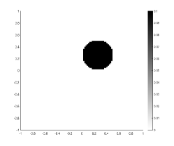
(c) Exact $\mu$

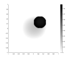
(d) Reconstructed $\mu$

Figure 1: Test Case 1-Reconstructions of the disk phantom with the 2PPAT-SR framework

From Figure 1b and 1d, we see that the reconstructions of both $\sigma$ and $\mu$ are of high resolution and high contrast. The value small shaded region around the disk in the reconstruction of $\mu$ is close to 0.02 and, thus, we only encounter a miniscule loss of contrast.

In test case 2, we consider a heart lung phantom for both $\sigma$ and $\mu$. For $\sigma$, the background value of the phantom is 0 that is perturbed into two ellipses that represent the lungs with value 1 and into a disk representing heart with value 0.5. The value of $\mu$ inside the ellipses and the disk is computed as $\mu=0.1\sigma$. The plots of the exact and the reconstructed phantoms are shown in Figure 2.

(a) Exact $\sigma$

(b) Reconstructed $\sigma$

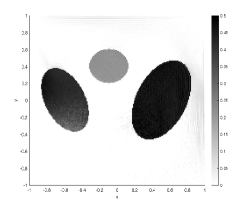
(c) Reconstructed $\sigma$ with 20%

(d) Exact $\mu$

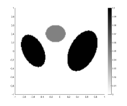
(e) Reconstructed $\mu$

(f) Reconstructed $\mu$ with 20% noise

Figure 2: Test Case 2-Reconstructions of the heart and lung phantom with the 2PPAT-SR framework

We again see from Figures 2b and 2e that the reconstructions of $\sigma,\mu$ are of high contrast and high resolution. To test the robustness of our method, we add 20% multiplicative Gaussian noise to the interior data $\mathcal{H}^{\sigma,\mu}$ and use it for our 2PPAT-SR inversion algorithm. We also modify the value of the regularization parameters $\xi_{1}=0.1,\xi_{2}=0.1,\gamma_{1}=0.3,\gamma_{2}=0.3$, in order to counter the noisy data. The results can be seen in Figure 2c and 2f. We see that the reconstruction of $\sigma$ contains a few artifacts but still is of good quality. The reconstruction of $\mu$ demonstrates very little artifacts. This shows that our 2PPAT-SR reconstruction framework is robust and accurate even in the presence of noisy data.

In test case 3, we consider $\sigma$ as the Shepp-Logan phantom given in [25]. The background $\sigma_{b}$ is chosen to be 0.3 in this case. We compute $\mu=0.1\sigma$ and the background value of $\mu_{b}$ is chosen as 0.03. The plots of the exact and reconstructed phantoms are shown in Figure 3.

(a) Exact $\sigma$

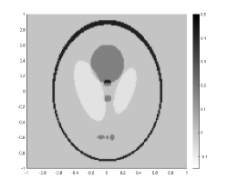
(b) Reconstructed $\sigma$

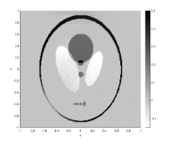
(c) Reconstructed $\sigma$ with 20% noise

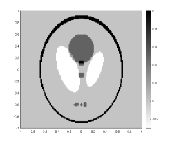
(d) Exact $\mu$

(e) Reconstructed $\mu$

(f) Reconstructed $\mu$ with 20% noise

Figure 3: Test Case 3-Reconstructions of the Shepp-Logan phantom with the 2PPAT-SR framework

We again see from Figures 3b and 3e that the 2PPAT-SR reconstruction framework gives superior quality reconstructions even for objects with high contrast values and with holes and inclusions. The reconstructions with 20% noise in the interior data are shown in Figures 3c and 3f with the modified regularization parameter values as in the previous test case. We see that the reconstructions are still of high quality with very less artifacts.

6 Conclusions

In this work, we have presented a new reconstruction framework for determining the optical coefficients in two-photon PAT. The framework comprises of a PDE-constrained optimization problem that promotes sparsity patterns in the reconstructions of the single and two photon absorption coefficients. We present a new theoretical analysis of the existence and uniqueness of a solution to a semi-linear elliptic PDE arising in 2P-PAT. Further, we present a proximal scheme using a Picard solver for the semi-linear PDE and its adjoint to solve the optimization problem. Several numerical results demonstrate that the proposed framework is able to achieve reconstructions with high contrast and high resolution for objects including holes and inclusions.

7 Acknowledgments

The authors are grateful to Gaik Ambartsoumian for several fruitful and important suggestions. S. Roy was partly supported by the National Cancer Institute, National Institutes of Health, grant number: 1R21CA242933-01.

References

• [1] B. J. Adesokan, K. Knudsen, V. P. Krishnan and S. Roy. A fully non-linear optimization approach to acousto-electric tomography. Inverse Problems, 34(10), 2018.
• [2] H. Ammari. An introduction to mathematics of emerging biomedical imaging. Mathematics and Applications, Springer, Berlin, Vol. 62, 2008.
• [3] G. Bal. Hybrid inverse problems and internal functionals. Inside Out II, Mathematical Sciences Research Institute Publications, Cambridge University Press, Vol. 60, 2012.
• [4] G. Bal and K. Ren. Multiple-source quantitative photoacoustic tomography in a diffuse regime. Inverse Problems, 27(7):075003, 2011.
• [5] G. Bal and G. Uhlmann. Inverse diffusion theory of photoacoustics. Inverse Problems, 26(8):085010, 2010.
• [6] P. Bardsley, K. Ren and R. Zhang. Quantitative photoacoustic imaging of two-photon absorption. Journal of Biomedical Optics, 23(1):016002, 2018.
• [7] H. Brezis. Functional analysis, Sobolev spaces and partial differential equations. Universitext, Springer, New York, 2011.
• [8] W. Denk, J. H. Strickler and W. W. Webb. Two-photon laser scanning fluorescence microscopy. Science, 248(4951), pp. 73-76, 1990.
• [9] I. Ekeland and R. Témam. Convex analysis and variational problems. SIAM Classics in Applied Mathematics, 1999.
• [10] L. C. Evans. Partial differential equations. Graduate Studies in Mathematics, American Mathematical Society, Providence, RI, 1998.
• [11] A. R. Fisher, A. J. Schissler, and J. C. Schotland. Photoacoustic effect for multiply scattered light. Physical Review E, Statistical, Nonlinear, and Soft Matter Physics, 76(3):036604, 2007.
• [12] M. Gupta, R. K. Mishra and S. Roy. Sparse reconstruction of log-conductivity in current density impedance tomography. Journal of Mathematical Imaging and Vision. Vol. 62, pp. 189-205, 2020.
• [13] P. Kuchment. Mathematics of hybrid imaging, a brief review. The Mathematical Legacy of Leon Ehrenpreis, Springer Proceedings in Mathematics, Vol 16. Springer, Milano, 2012.
• [14] P. Kuchment and L. Kunyansky. Mathematics of thermoacoustic and photoacoustic tomography. Handbook of Mathematical Methods in Imaging, Springer 817-866, 2010.
• [15] P. Kuchment and D. Steinhauer. Stabilizing inverse problems by internal data. Inverse Problems, 28(8):084007, 2012.
• [16] O. A. Ladyzhenskaya and N. N. Uraltseva. Linear and Quasilinear Elliptic Equations. Academic press, New York and London, 1968.
• [17] Y. H. Lai, S. Y. Lee, C. F. Chang, Y. H. Cheng and C. K. Sun. Nonlinear photoacoustic microscopy via a loss modulation technique: from detection to imaging. Optics Express. 22(1), pp. 525-536, 2014.
• [18] G. Langer, K. D. Bouchal, H. Grün, P. Burgholzer and T. Berer. Two-photon absorption-induced photoacoustic imaging of Rhodamine B dyed polyethylene spheres using a femtosecond laser. Optics Express. 21, pp. 22410–22422, 2013.
• [19] C. Li and L. V. Wang. Photoacoustic tomography and sensing in biomedicine. Physics in Medicine and Biology, 54(19):R59-97, 2009.
• [20] M. Li. H. Yang and H. Kudo. An accurate iterative reconstruction algorithm for sparse objects: application to 3D blood vessel reconstruction from a limited number of projections. Physics in Medicine and Biology, 47(15):2599-2609, 2002.
• [21] K. Ren and R. Zhang. Nonlinear quantitative photoacoustic tomography with two-photon absorption. SIAM Journal on Applied Mathematics, 78(1):479–503, 2018.
• [22] S. Roy, M. Annunziato and A. Borzì. A Fokker-Planck feedback control-constrained approach for modelling crowd motion. Journal of Computational and Theoretical Transport, 45(6):442–458, 2016.
• [23] S. Roy, M. Annunziato, A. Borzì and Christian Klingenberg. A Fokker-Planck approach to control collective motion. Computational Optimization and Applications, 69(2):423–459, 2018.
• [24] S. Roy and A.Borzì. A new optimisation approach to sparse reconstruction of log-conductivity in acousto-electric tomography. SIAM Journal on Imaging Sciences, 11(2):1759–1784, 2018.
• [25] L. A. Shepp and B. F. Logan. The Fourier reconstruction of a head section. IEEE Transactions on Nuclear Science, 21(3):21–43, 1974.
• [26] G. Stadler. Elliptic optimal control problems with $L^{1}$-control cost and applications for the placement of control devices. Computational Optimization and Applications, 44(2):159–181, 2009.
• [27] P. T. C. So. Two-photon fluorescence light microscopy. Encyclopedia of Life Sciences, Nature Publishing Group, London, 2002.
• [28] B. E. Urban, J. Yi, V. Yakovlev and H. F. Zhang. Investigating femtosecond-laser-induced two-photon photoacoustic generation. Journal of Biomedical Optics, 19(8):085001, 2014.
• [29] T. Vu, D. Razansky and J. Yao. Listening to tissues with new light: recent technological advances in photoacoustic imaging. Journal of Optics, 21(10), 2019.
• [30] L. V. Wang. Ultrasound-mediated biophotonic imaging: a review of acousto-optical tomography and photoacoustic tomography. Disease Markers. Vol. 19 123-138, 2004.
• [31] L. V. Wang. Tutorial on Photoacoustic Microscopy and Computed Tomography. IEEE Journal of Selected Topics in Quantum Electronics. 14(1), 2008.
• [32] Y. Xu, L. V. Wang, G. Ambartsoumian and P. Kuchment. Reconstructions in limited view thermoacoustic tomography. Medical Physics 31(4), 724-733, 2004.
• [33] Y. Xu, L. V. Wang, G. Ambartsoumian and P. Kuchment. Limited view thermoacoustic tomography. Photoacoustic Imaging and Spectroscopy, CRC Press, 61-73, 2009.
• [34] M. Xua and L. V. Wang. Photoacoustic imaging in biomedicine. Review of Scientific Instruments, Vol. 77: 041101, 2006.
• [35] Y. Yamaoka, Y. Kimura, Y. Harada, T. Takamatsu and E. Takahashi. Fast focus-scanning head in two-photon photoacoustic microscopy with electrically controlled liquid lens. Photons Plus Ultrasound: Imaging and Sensing Vol. 10494, 2018.
• [36] Y. Yamaoka, M. Nambu, and T. Takamatsu. Frequency-selective multiphoton excitation induced photoacoustic microscopy (MEPAM) to visualize the cross sections of dense objects. Photons Plus Ultrasound: Imaging and Sensing, Vol. 756420, 2010.
• [37] Y. Yamaoka, M. Nambu, and T. Takamatsu. Fine depth resolution of two-photon absorption-induced photoacoustic microscopy using low-frequency bandpass filtering. Optics Express, Vol. 19, pp. 13365-13377, 2011.
• [38] Y. Yamaoka and T. Takamatsu. Enhancement of multiphoton excitation-induced photoacoustic signals by using gold nanoparticles surrounded by fluorescent dyes. Photons Plus Ultrasound: Imaging and Sensing, Vol. 71772A, 2009.
• [39] J. Ying, F. Liu, and R. R. Alfano. Spatial distribution of two-photon-excited fluorescence in scattering media. Applied Optics,38(1), pp. 224-229, 1999.
• [40] W. R. Zipfel, R. M. Williams and W. W. Webb. Nonlinear magic: multiphoton microscopy in the biosciences. Nature Biotechnology Vol. 21, pp. 1369-1377, 2003.