New Framework for Code-Mapping-based Reversible Data Hiding in JPEG Images

Abstract

Code mapping (CM) is an efficient technique for reversible data hiding (RDH) in JPEG images, which embeds data by constructing a mapping relationship between the used and unused codes in the JPEG bitstream. This study presents a new framework for designing a CM-based RDH method. First, a new code mapping strategy is proposed to suppress file size expansion and improve applicability. Based on our proposed strategy, the mapped codes are redefined by creating a new Huffman table rather than selecting them from the unused codes in the original Huffman table. The critical issue of designing the CM-based RDH method, that is, constructing code mapping, is converted into a combinatorial optimization problem. This study proposes a novel CM-based RDH method that utilizes a genetic algorithm (GA). The experimental results demonstrate that the proposed method achieves a high embedding capacity with no signal distortion while suppressing file size expansion.

1 Introduction

Reversible data hiding (RDH) is a technique that can imperceptibly embed additional data into media and then restore the media error-free. The past decades have witnessed the rapid development of RDH techniques in different application scenarios, such as remote sensing, medical image processing, and image authentication [1]. Many RDH methods have been developed for uncompressed images, including lossless compression [2][3], difference expansion (DE) [4][5], histogram shifting (HS) [6, 7, 8], and prediction error expansion (PEE) [9, 10, 11, 12].

JPEG RDH research has attracted considerable attention in recent years because JPEG is the most commonly used image compression format in applications. JPEG RDH methods mainly focus on two aspects: modifying the quantized discrete cosine transform (DCT) coefficients [13, 14, 15, 16, 17, 18, 19, 20, 21, 22, 23, 24, 25, 26, 27] and manipulating the JPEG bitstream [28, 29, 30, 31, 32, 33, 34]. The first type of methods, which focus on DCT coefficients are mainly based on lossless compression [13, 14, 15], zero-run value (ZRV) pair rotation [16, 17], and HS [18, 19, 20, 21, 22, 23, 25, 24, 26, 27]. Because the DCT coefficients are modified directly during data embedding, these RDH methods cause file size expansion and image distortion. Among the aforementioned methods, HS-based methods [18, 19, 20, 21, 22, 23, 25, 24, 26, 27], which focus on the modification of DCT coefficients to balance signal quality and file size preservation, have been the most widely studied.

The second type of JPEG RDH methods is mainly based on code mapping (CM) [28, 29, 30, 31, 34, 32, 33], which embeds data by building the mapping between used variable length codes (VLC) and unused VLCs in the JPEG bitstream. In [35], data were embedded into the bitstream by flipping one bit of the code. Mobasseri et al. applied an error concealment technique to minimize image quality distortion. Inspired by previous research [35], Qian and Zhang [28] mapped used VLCs with several unused VLCs of identical lengths, guaranteeing no quality distortion and preserving the file size of the bitstream. Subsequently, a number of CM-based RDH methods [29, 30, 31] aimed to improve the capacity while keeping the length of the marked JPEG bitstream unchanged. Several CM-based methods [34, 32, 33] have recently attempted to improve capacity by undermining file size increments. Qiu et al. [32] first employed a relay-transfer-based algorithm to preprocess the JPEG bitstream and then embedded data into the processed bitstream to improve its capacity. Du et al. [33] proposed the reordering of run-size values and established a simulated embedding model to find a better mapping relationship. Zhang et al. [34] utilized a value transfer matrix to simulate a theoretical model and designed optimization rules to build a mapping relationship.

In general, CM-based RDH studies [28, 29, 30, 31, 34, 32, 33] have two major advantages. On the one hand, CM-based RDH methods hide the secret bits directly into the bitstream without modifying the DCT coefficients; thus, no distortion is generated. Therefore, the image restoration process can be canceled after data extraction, because the image content remains unchanged after data embedding. On the other hand, it is more efficient because CM-based methods require neither full decompression nor recompression. Therefore, the CM technique is a better choice among existing approaches for JPEG RDH.

However, some problems in CM-based JPEG RDH research still exist. First, previous CM-based methods [28, 29, 30, 31, 34, 32, 33] rarely consider file size as an optimization goal during code mapping construction. However, file size preservation is considered a critical issue when designing a satisfactory JPEG RDH method. Although recent CM-based studies [34, 32, 33] achieved high embedding capacities, the file size also increased as the capacity increased. Second, the aforementioned CM-based RDH methods [28, 29, 30, 31, 34, 32, 33] apply only to the bitstream encoded with the standard Huffman table (hereafter referred to as std-bitstream). With the massive number of images growing on the Internet, the bitstream encoded with the optimized Huffman table (hereafter referred to as opt-bitstream) is preferred over the std-bitstream because it requires less storage space. In contrast to the std-bitstream, all VLCs in the opt-bitstream are used; therefore, the code mapping cannot be constructed. This means that the aforementioned CM-based methods [28, 29, 30, 31, 34, 33, 32] are unavailable in the opt-bitstream.

In this study, we proposed a novel framework for designing a CM-based RDH method that achieves good file size preservation performance, and demonstrated it with a novel CM-based RDH method. The main contributions of this study are summarized as follows:

• A new code mapping strategy is proposed to improve file size preservation and applicability performance.

• A new framework to design a CM-based method is provided. Under this framework, the critical issue of the CM-based method, i.e., code mapping construction, is converted into solving a combinatorial optimization problem with different given constraints.

• As a realization of the proposed framework, a novel CM-based JPEG RDH method is proposed by employing a genetic algorithm (GA) to solve the optimization problem.

• Comprehensive experiments demonstrate that the proposed method effectively suppresses the file size expansion compared to previous CM-based RDH methods and HS-based RDH methods.

The remainder of this paper is organized as follows. Section 2 provides an overview of the JPEG bitstream structure and the basic CM-based RDH method. Section 3 describes the proposed code-mapping strategy. Section 4 presents a detailed universal framework. Section 5 presents the new CM-based RDH method, Section 6 describes the experimental results, and Section 7 concludes the paper.

2 Background

In this section, we first introduce the baseline JPEG bitstream structure. We then briefly present the traditional CM-based RDH framework.

2.1 JPEG bitstream structure

For brevity, we only introduce the syntax of the JPEG baseline for grayscale images. The JPEG bitstream consists of a file header and entropy-coded data, as shown in Fig. 1. A JPEG bitstream starts with the marker start-of-image (SOI) and ends with the marker end-of-image (EOI). There are several segments between SOI and EOI, including the define Huffman table (DHT) segment and the start-of-scan (SOS) segment related to the CM-based RDH.

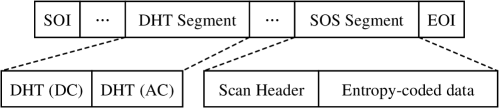
Figure 1: JPEG bitstream structure.

As described in the JPEG standard [36], the quantized AC coefficients are first compressed into the form of $(run/size,value)$. $value$ is the amplitude of the next non-zero AC coefficient, which is further encoded, and the generated codes are referred to as appended bits. Each symbol $run/size$ (RS) is encoded using a unique VLC. Fig. 2 presents the DHT segment containing the RS information to construct the Huffman table. As shown in Fig. 2, the DHT segment mainly includes two lists: BITS and HUFFVAL. The BITS list contains VLCs of different lengths. For example, the first byte “00” means the code length of one is zero. The HUFFVAL list contains the hexadecimal forms of the RSs. For example, the first RS “0/1” is recorded as 0x01. In a std-bitstream, the HUFFVAL list occupied 162 bytes, covering all 162 RSs. Each RS in the HUFFVAL list corresponds to one VLC defined in the standard Huffman table. However, the size of the HUFFVAL list in the opt-bitstream depends on nonzero-frequency RSs (NFRS). A Huffman table can be constructed based on these two lists. The SOS segment includes a scan header and entropy-coded data. The entropy-coded data include the compressed forms of the DC and AC coefficients, that is, the VLCs and appended bits, respectively.

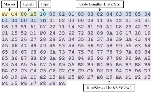
Figure 2: DHT Segment for AC coefficients contains the standard Huffman table information defined in the JPEG standard [36]. 0xFFC4 is the marker that represents the DHT segment. 0x00B5 denotes the segment length except for the marker 0xFFC4, which equals to B5${}_{(16)}=181$ bytes. 0x10 specifies the type of DHT segment for AC coefficients. The lists BITS and HUFFVAL record the Huffman table information.

2.2 Traditional CM-based RDH framework

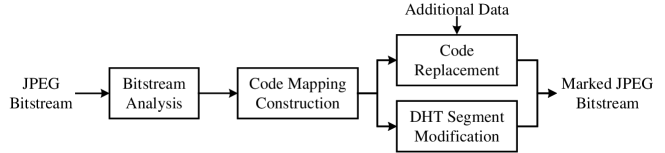
Figure 3: Traditional framework of CM-based JPEG RDH.

The traditional CM-based RDH framework is depicted in Fig. 3. In the bitstream analysis phase, the JPEG bitstream is parsed and all VLCs are constructed according to the DHT segment. Then, the occurrence of each VLC used in the entropy-coded data was calculated. In the code-mapping construction phase, some mapping rules are designed to construct code mappings between the used and unused VLCs. Early file-size-preserving CM-based methods [28, 29, 30, 31] mapped the used VLC to unused VLCs with the same code lengths to ensure that the file size of the bitstream remained invariant, causing limited embedding capacity. To improve the capacity, recent CM-based RDH research [28, 29, 30, 31] built a mapping among VLCs across different code lengths. After determining the code mapping relationship, additional data can be embedded by replacing the used VLCs with VLCs in the same mapping set. To maintain the decoded image pixels unchanged after embedding, the zero-frequency RS (ZFRS) of the corresponding VLC in the same mapping set is replaced by the NFRS in the DHT segment.

3 Proposed code mapping strategy

During the code mapping construction, previous CM-based studies [28, 29, 30, 31, 34, 33, 32] directly select the required VLCs from existing unused VLCs and map them to used VLCs. We refer to this code-mapping strategy as the traditional code-mapping strategy. With the traditional mapping strategy, during the DHT segment modification, the selected ZFRSs are substituted by NFRSs to represent the mapping relationship, and the selected ZFRSs remain unchanged. This means that the Huffman table constructed using the modified DHT segment remains similar to the standard Huffman table. However, the standard Huffman table is defined by the average statistics obtained from a large collection of data, which does not exactly match the actual distribution of RSs in a JPEG bitstream; thus, coding redundancy exists. Recent CM-based RDH studies [28, 29, 30, 31] achieved a high embedding capacity by constructing mappings among VLCs across different code lengths. These studies used a traditional code-mapping strategy. Although these studies proposed some means to control file size expansion, the file size increment is still apparent.

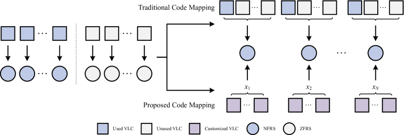
Figure 4: Difference between traditional code mapping strategy and our proposed code mapping strategy. In the proposed strategy, the required VLCs are all customized and mapped to NFRSs, rather than being selected from the standard Huffman table as in previous CM-based methods. Therefore, the proposed code mapping strategy applies to both the std-bitstream and opt-bitstream.

To further suppress the file size expansion, we propose a new code mapping strategy to guide the construction of the mapping relationship. The idea of the proposed strategy is to redefine the required VLCs, that is, all the VLCs used to construct the mapping relationship, by thoroughly customizing the Huffman table and mapping them to NFRSs. The difference between the traditional code mapping strategy and the proposed code mapping strategy is shown in Fig. 4. In the proposed strategy, each NFRS can be mapped using multiple VLCs. Instead of the Huffman table in the original JPEG bitstream, the required VLCs only depend on the distribution of NFRSs and the given constraints during the data embedding; therefore, the method designed based on the proposed strategy applies to both the opt-bitstream and std-bitstream. During the DHT segment modification, we added several copies of the original NFRSs to the HUFFVAL list, which is necessary for constructing the code mapping. Because only the necessary RSs are stored in the DHT segment, the Huffman table constructed using the customized DHT segment is similar to the optimized Huffman table. Therefore, coding redundancy can be significantly reduced; thus, the file size will be well preserved.

4 New framework for CM-based RDH

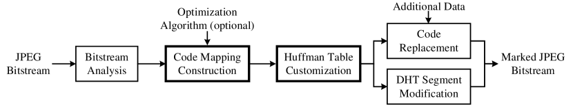
Figure 5: New framework of CM-based JPEG RDH.

The proposed framework for CM-based RDH is shown in Fig. 5. First, the original Huffman table was constructed by parsing the BITS and HUFFVAL lists in the DHT segment. Using the original Huffman table, the occurrences of the used VLCs in the entropy-coded data were calculated, and the statistical results of the RS frequency were obtained. According to the RS frequency and given constraints, the NFRSs were mapped with multiple VLCs adaptively to construct an optimal code mapping relationship. In the proposed framework, the code mapping construction is formulated as a combinatorial optimization problem and can be solved by leveraging optimization algorithms. We then constructed a customized Huffman table according to the optimal solution. The additional data were then embedded into the entropy-coded data by replacing the original VLCs and modifying the DHT segment. Finally, the marked JPEG bitstream was synthesized from the new entropy-coded data and new file header. The marked JPEG bitstream can still be decoded directly using the most widely used decoders.

Compared with the traditional framework of CM-based JPEG RDH, the proposed framework has two key issues. The first issue is to determine the number of VLCs mapped to each NFRS under the given constraints. To address this issue, we formulated the code-mapping construction as a combinatorial optimization problem, which can be solved using the optimization algorithm, as discussed in Section 4.1. The second issue is the process of Huffman table customization, which is detailed in Section 4.2.

4.1 Code mapping construction

According to the proposed code mapping strategy, it is possible for each NFRS to be mapped to multiple VLCs. For ease of description, we introduced a $1\times N$ sequence called the mapping sequence as $\bm{x}=(x_{1},x_{2},\dots,x_{N})$, where $N$ is the number of NFRSs in the original bitstream, and $x_{i}$ represents the number of VLCs mapped to the $i$-th NFRS. The mapping sequence $\bm{x}$ can be used to represent the constructed code mapping. Therefore, constructing an optimal code mapping is equivalent to finding the optimal mapping sequence, which can be considered a combinatorial optimization problem with constraints. The optimization objective is to minimize the file size increment with respect to the required capacity. A key constraint is that the capacity calculated by the mapping sequence $\bm{x}$ must be greater than or equal to the required capacity. In addition, according to the Huffman coding rules of the JPEG standard [36], two other constraints must be considered.

1. For each NFRS, at least one VLC must be mapped to provide error-free encoding and decoding. Therefore, each element in the mapping sequence $\bm{x}$ must be an integer greater than or equal to one.

2. According to Section K.2 in the JPEG standard [36], the number of customized VLCs, i.e., the sum of mapping sequence $\bm{x}$, can be up to 256. Therefore, the sum of $\bm{x}$ has a range of $N$ to 256.

Let $z$ denote the required capacity, the optimization problem can be formulated as

$$\begin{split}&\mathrm{minimize}\ \ \ \mathcal{F}(\bm{x})\\ &\mathrm{subject\ to}\ \begin{cases}\mathcal{C}(\bm{x})\geq z&\\ x_{i}\geq 1,i\in[1,N]&\\ \sum_{i=1}^{N}x_{i}\leq 256\end{cases}\end{split},$$ (1)

where $\mathcal{F}(\bm{x})$ represents the file size of the part of marked bitstream that will change with different mapping sequences. Thus, minimizing the file size increment is equivalent to determining a mapping sequence with a minimal value of $\mathcal{F}(\bm{x})$. $\mathcal{C}(\bm{x})$ represents the embedding capacity achieved by the mapping sequence $\bm{x}$, which can be calculated as

$$\mathcal{C}(\bm{x})=\sum_{i=1}^{N}f_{i}\cdot\left\lfloor\log_{2}x_{i}\right\rfloor,$$ (2)

where $f_{i}$ denotes the frequency of $i$-th NFRS in the original bitstream, and $\left\lfloor\cdot\right\rfloor$ is the floor operator.

In the workflow of the proposed framework, only the DHT segment and the entropy-coded data are changed; therefore, we only need to compare the file size change in the two parts. We note that when calculating the file size increment, the file size changed owing to byte alignment, and zero-byte padding was not included because the modification could not be calculated before ending the encoding, and it was extremely small that it could be negligible.

4.1.1 File size change in the DHT segment

The file size change in the DHT segment occurs in the DHT segment modification step, which is caused by adding the copies of the NFRSs to the HUFFVAL list to represent the code mapping. The original lists, BITS and HUFFVAL, were replaced with the lists generated during the DHT segment modification. Fig. 6 presents an example of the DHT segment before and after modification. As shown in Fig. 6, the segment length is changed from 0x0046 to 0x0048, which means the file size increment in the DHT segment is 16 bits. In this example, the RSs “2/1” and “2/2” are added to one copy to construct the code mapping. Therefore, in the HUFFVAL list, two extra RSs are added, which are marked in red. The BITS list was also modified to generate a customized Huffman table. We note that the values of the other RSs in the HUFFVAL list remained unchanged; however, the positions were adjusted to improve the compression ratio.

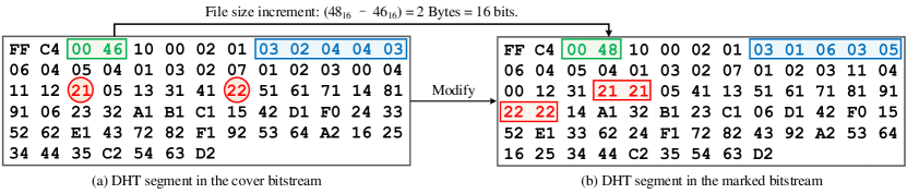
Figure 6: Comparison of the DHT segment before and after modification. The segment length is changed from 0x0046 to 0x0048, which are marked in green. In the BITS list, five bytes are modified, which are marked in blue. In the HUFFVAL list, two RSs, “2/1” and “2/2”, are assigned with two VLCs to construct the code mapping, which are marked in red.

As the file sizes of other parts in the DHT segment are unchanged, calculating the file size change in the DHT segment is equivalent to calculating the file size of the new HUFFVAL list (in bits). Let $N^{\prime}$ denote the number of customized VLCs, which is calculated as

$$N^{\prime}=\sum_{i=1}^{N}x_{i}.$$ (3)

Because an RS occupies one byte (8 bits) of space in the HUFFVAL list, the file size change in the DHT segment $\mathcal{F}_{\mathrm{huffval}}$ can be calculated by

$$\mathcal{F}_{\mathrm{huffval}}=8N^{\prime}.$$ (4)

4.1.2 File size change in the entropy-coded Data

The file size change in the entropy-coded data is caused by VLC replacement. During the VLC replacement, all the original VLCs are substituted by the VLCs defined by the customized Huffman table. Thus, calculating the file size change in entropy-coded data is equivalent to calculating the file size of VLCs after replacement based on the customized Huffman table. However, customizing the Huffman table requires determining the optimal mapping sequence and, thus, the customized Huffman table cannot be obtained during the code mapping construction step. To this end, we propose a surrogate method from the perspective of information theory, which can approximate the file size of VLCs without a customized Huffman table.

According to information theory, the length of a VLC is close to its self-information (in bits) as the VLC is a Huffman code. Therefore, we can obtain the approximate length of the VLC by calculating its self-information. Calculating self-information requires the actual post-embedding frequency of VLCs. Considering that the actual post-embedding frequency cannot be obtained before data embedding, the post-embedding frequency can be estimated as follows:

$$f_{i}^{\prime}\approx\left\{\begin{array}[]{ll}f_{1}/x_{1},&\text{ if }1\leqslant i\leqslant x_{1}\\ f_{2}/x_{2},&\text{ if }x_{1}<i\leqslant x_{1}+x_{2}\\ \cdots\\ f_{N}/x_{N},&\text{ if }\sum_{j=1}^{N-1}x_{j}<i\leqslant N^{\prime}\end{array}\right.,$$ (5)

where $f_{i}^{\prime}$ represents the estimated post-embedding frequency of the $i$-th VLC in the customized Huffman table. This estimation is based on the fact that additional data are encrypted before embedding. That means the “0” and “1” in the additional data are distributed equally; therefore, the frequency of each VLC mapped to the same NFRS will be approximately identical.

The self-information of the $i$-th VLC $I_{i}$ can therefore be calculated as

$$I_{i}=\log_{2}\left(\frac{\sum_{j=1}^{N^{\prime}}f_{j}^{\prime}}{f_{i}^{\prime}}\right).$$ (6)

Finally, the file size of the VLCs, namely, $\mathcal{F}_{\mathrm{vlc}}$, can be estimated as

$$\begin{split}\mathcal{F}_{\mathrm{vlc}}&=\sum_{i=1}^{N^{\prime}}I_{i}\cdot f_{i}^{\prime}=\sum_{i=1}^{N^{\prime}}\log_{2}\left(\frac{\sum_{j=1}^{N^{\prime}}f_{j}^{\prime}}{f_{i}^{\prime}}\right)\cdot f_{i}^{\prime}.\end{split}$$ (7)

In Eq. (7), we multiply the estimated post-embedding frequency of VLC with its corresponding self-information and sum it to approximate the actual file size of VLCs.

According to Eqs. (4) and (7), the function $\mathcal{F}(\bm{x})$ can be written as:

$$\begin{split}\mathcal{F}(\bm{x})&=\mathcal{F}_{\mathrm{huffval}}+\mathcal{F}_{\mathrm{vlc}}.\\ \end{split}$$ (8)

4.2 Huffman Table Customization

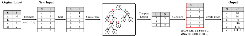
Figure 7: Example to generate the customized Huffman table. S: RS. F: frequency. L: length of VLC. N: number of VLC with the same length. C: VLC.

Because the number of customized VLCs is flexible, the Huffman table customization step is different from previous CM-based methods; however, it is similar to the generation of the optimized Huffman table. The difference is that we considered the estimated post-embedding frequency as the input instead of the original RS frequency. Fig. 7 depicts a simplified example to illustrate the generation of the customized Huffman table. We note that a detailed version of the generation of the Huffman table can be found in Section K.2 of the JPEG standard [36]. First, the original RS and corresponding frequency are transformed into a 2-tuple sequence $\{(a,10),(b,3),(c,2),(d,2)\}$ to generate a new input. Assuming that the mapping sequence is $\bm{x}=(2,1,2,1)$, the new 2-tuple sequence is then generated by estimating the post-embedding frequency, that is, $\{(a,5),(a,5),(b,3),(c,1),(c,1),(d,2)\}$. After sorting the RSs according to frequency, the Huffman tree was created and used to compute the code lengths. The codes were then canonized to create a canonical Huffman code. Canonical Huffman code lengths were recorded on the BITS list. As shown in Fig. 7, the numbers of code lengths 2, 3, 4, and 5 are 3, 1, 1, and 1, respectively. Therefore, the BITS list is “00 03 01 01 01…”. Next, a high-frequency RS is assigned with a short code to compress the bitstream. The HUFFVAL list was created according to the code length. These two lists were used to generate a customized Huffman table.

5 Example: a new CM-based RDH method

This section presents a new CM-based RDH method to realize the proposed framework. First, a GA is introduced to solve the optimization problem; thus, a nearly optimal code mapping is constructed. Then, the data embedding and extraction procedures are described.

5.1 Problem solving using GA

Input:

 Population size $K$, iterations $I$, crossover rate $R_{c}$,

 and mutation rate $R_{m}$

Output:

 The best individual $p^{*}$

1 Generate the initial parent population of $K$ individuals, $P=\{p_{1},p_{2},\dots,p_{K}\}$;

2 for $i=1$ to $I$ do

3       Compute the fitness of each $p_{i}\in P$;

4       Find the best individual and define it as $p^{*}$;

5       Insert $p^{*}$ into the new population $P^{\prime}$. Select $K-1$ individuals from $P$ for reproduction. ;

6       The crossover operation is performed based on $R_{c}$. Perform a mutation operation based on $R_{m}$;

7       Insert the new $K-1$ individuals into $P^{\prime}$;

8       $P\leftarrow P^{\prime}$;

9      

10 end for

return $p^{*}$

Algorithm 1 GA procedure

Evaluating all mapping sequences is impractical, because the solution space is very large. Thus, designing a fast and effective optimization algorithm is vital for searching for a nearly optimal solution. We leveraged the GA to automatically search for a nearly optimal solution. We designed several specific problem-oriented rules to improve search accuracy and convergence speed. Algorithm 1 describes the GA procedure. In this algorithm, $K$ individuals are randomly generated to initialize the parent population $P=\{p_{1},p_{2},\dots,p_{K}\}$. Subsequently, the fitness of each individual in $P$ was computed. To complete the reproduction of the new population, GA operations (i.e., selection, crossover, and mutation) were performed to generate new individuals. The reproduction of the new population terminates when the maximum number of iterations $I$ is reached.

5.1.1 Population initialization

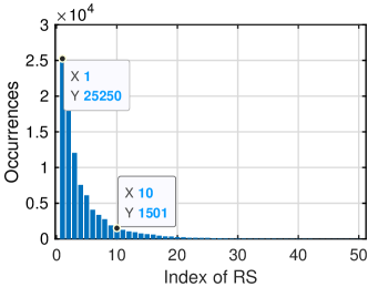
Figure 8: Distribution of RSs of the Baboon image under a QF of 70.

One mapping sequence $\bm{x}$ is regarded as an individual of a population. This means that $N$ genes are encoded in an individual when the number of NFRSs is $N$. Each gene corresponds to an element in mapping sequence $\bm{x}$. However, not all NFRSs are suitable for assigning multiple VLCs. Some low-frequency RSs contribute only to the limited embedding capacity when mapping multiple VLCs to them. Fig. 8 illustrates the RS frequency of the image Baboon with a quality factor (QF) of 70. As shown in Fig. 8, the frequencies of most RSs are low and not suitable for constructing code mapping when embedding a large payload of additional data. When searching for a nearly optimal solution, these RSs will occupy a portion of the available VLCs and influence the convergence speed. With this concern in mind, we selected a certain number of RSs to construct code mapping rather than all RSs. After several preliminary trials (not reported here), we finally considered ten as the number in the proposed method. We limited the selected 10 RSs to consecutive ones, where the leftmost one was closest to and greater than the required capacity. The RSs may encounter the following situations:1) less than 10 RSs are available and 2) the leftmost RS is smaller than the required capacity. When the number of RSs is less than 10, all RSs are selected. When the leftmost capacity is less than the required capacity, the RS is selected starting from the leftmost one. l

5.1.2 Individual encoding

To solve the optimization problem using the GA, all the tunable parameters in an individual, i.e., the mapping sequence $\bm{x}=(x_{1},x_{2},\dots,x_{N})$ should be represented with binary encoding. Considering that using three or more bits to represent an element in $\bm{x}$ will decelerate the convergence and produce more infeasible solutions, we limit the value of each $x_{i}$ to one in $\{1,2,4,8\}$ to reduce the solution space. Each value in $\{1,2,4,8\}$ occupies two bits, such as the codes “00”, “01”, “10”, and “11”, which are used to represent 1, 2, 4, 8, respectively. Based on this rule, one VLC can represent up to three bits of data ($\log_{2}8$). Thus, an individual is composed of a sequence of 20 bits. Therefore, the $i$th individual, $p_{i}$ in the population can be represented by

$${p_{i}}=\{a_{1}^{1}a_{1}^{2}\cdots a_{10}^{1}a_{10}^{2}\mid a_{j}^{1},a_{j}^{2}\in\{0,1\}\ \text{and}\ j\in[1,10]\},$$ (9)

where $(a_{j}^{1},a_{j}^{2})$ represents the $j$-th genes in an individual.

5.1.3 Selection, crossover, and mutation

In the reproduction process of the population, we adopted the elite preservation strategy. We inserted it into the new population for the best individual instead of modifying it. We used roulette wheel selection to select better individuals for the remaining individuals. After the crossover and mutation steps, the newly generated individuals are inserted into the next generation.

5.1.4 Fitness function

The fitness function is used to evaluate the quality of individuals. This eventually causes GA to evolve toward an individual with better fitness. According to the optimization problem formulated in Eq. (1), the optimal individual has the minimum value of $\mathcal{F}(\bm{x})$. However, roulette-wheel selection selects individuals with higher fitness values. Thus, we adjust the fitness value for the $i$th individual as follows:

$$fitness(i)=\mathcal{F}_{\mathrm{max}}-\mathcal{F}_{i},$$ (10)

where $\mathcal{F}_{\mathrm{max}}$ denotes the maximal value of $\mathcal{F}(\bm{x})$ in one generation, and $\mathcal{F}_{i}$ is the value of $\mathcal{F}(\bm{x})$ calculated by the $i$-th individual. The fitness value is set to zero as a penalty for an individual who does not satisfy the capacity constraint.

5.2 Data embedding & extraction

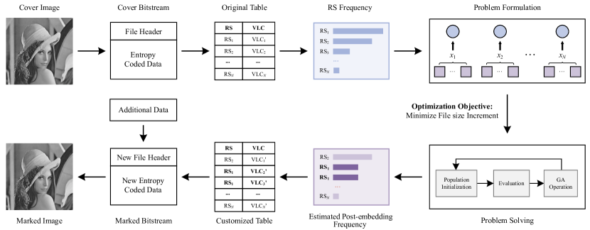
Figure 9: Embedding process of the proposed method.

Fig. 9 depicts the embedding procedures of the proposed method, which are as follows:

1. Construct the Huffman table by parsing the file header in the bitstream.

2. Count the RS frequency by parsing the entropy-coded data.

3. Convert the code mapping construction to a combinatorial optimization problem and solve it using the GA.

4. Calculate the estimated post-embedding frequency after obtaining the nearly optimal solution, and construct the customized Huffman table

5. Embed the additional data into the entropy-coded data and modify the file header.

6. Generate the marked JPEG bitstream by combining the new entropy-coded data with the new file header.

Fig. 10 depicts a basic data embedding example by code mapping. We assume that “0/6”, “1/3”, and “6/1” are all zero-frequency RSs. The corresponding VLCs are unused and can be used to construct mapping relationships. After modifying the three RSs to “5/1”, the code mapping is constructed, and each VLC represents two bits of different data. The additional data “011011” can then be embedded by replacing the original VLCs with VLCs in the mapping set.

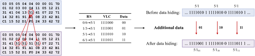
Figure 10: CM-based data embedding example.

The code mapping constructed in the data embedding process is required to extract the additional data embedded in the marked JPEG bitstream. Instead of solving the optimization problem, code mapping can be directly constructed by parsing the DHT segment during data extraction. The entropy-coded data are further parsed and additional data can then be extracted. Because the marked image is lossless to the original image in terms of the image quality, the image content does not need to be restored. The customized Huffman table must be replaced by different Huffman tables to restore the bitstream. The standard Huffman table can be found in the JPEG standard [36], and an optimized Huffman table can be generated according to the RS frequency. The main data extraction procedure is described as follows:

1. Generate the customized Huffman table for AC coefficients by parsing the DHT segment from the marked JPEG bitstream.

2. Construct the mapping relationship according to the customized Huffman table.

3. Extract the embedded data from the entropy-coded data according to the mapping relationship.

4. Synthesize a new JPEG bitstream using the optimized Huffman table or standard Huffman table.

6 Experimental results

In this section, we first introduce the experimental settings in Section 6.1. The results and comparisons with previous methods in terms of file size preservation, image quality, and running time are presented in Sections 6.2, 6.3, and 6.4, respectively.

6.1 Experimental settings

6.1.1 Datasets

The images tested in our experiments are selected from two commonly used image databases:

• USC-SIPI [37] is a collection of digitized images. We select four classical $512\times 512$ images, Lena, Elaine, Baboon, and Boat from this image database. These selected images after JPEG compression have a QF = 70. The four selected images can be classified into two categories. The first two images, Lena and Elaine, contain more low-frequency details and smooth areas. More high-frequency details and texture areas are contained in the other two images, Baboon and Boat.

• BOSSbase [38] consists of 10000 512 $\times$ 512 grayscale images in the PGM format. For follow-up experiments, 200 images from the BOSSbase image database were randomly selected.

Because the images in the two databases are uncompressed images, we converted all the selected images into grayscale JPEG images. To convert the image from the uncompressed format, TIFF or PGM, into the JPEG format, the MATLAB imwrite function was used. All JPEG images generated by the imwrite function were encoded using the standard Huffman table. To verify the applicability of our proposed method, the JPEG images encoded with the optimized Huffman table were regarded as the original images in our experiments. JPEG images encoded with the optimized Huffman table were generated using the jpeg_read and jpeg_write functions in the JPEG toolbox [39].

6.1.2 Evaluation metrics

To evaluate the performance of the proposed method, three criteria, including the file-size increment, the mean square error (MSE) and the running time, are employed:

• File-size Increment (FI) is the difference of file-sizes of the marked bitstream and the original bitstream, which is used to evaluate the file size preservation performance.

• Mean Square Error (MSE) is employed to evaluate the image quality of the marked JPEG image, which is calculated as

  $$MSE=\frac{1}{h\times w}{\sum_{i=1}^{h}}{\sum_{j=1}^{w}}\left(X_{i,j}-X^{\prime}_{i,j}\right)^{2},$$ (11)

  where $h$ and $w$ are the height and width of original JPEG image, respectively. $X_{i,j}$ and $X^{\prime}_{i,j}$ are the $(i,j)$-th pixel in original JPEG image and marked JPEG image, respectively. According to Eq. (11), the smaller MSE represents less distortion and better visual quality. When the MSE is equal to zero, the marked JPEG image is lossless compared to the original JPEG image.

• Running Time refers to the running time of the data embedding process. We use it to evaluate the complexity of our chosen methods. For a fair comparison, we tested all the methods in the same environment, including the software and hardware.

6.1.3 Baselines

To validate the effectiveness of our proposed method, three state-of-the-art high capacity CM-based RDH methods were selected for comparison, including method [32] (TCSVT2021), method [33] (TDSC2020), and method [34] (JVCIR2020). In [32], Qiu et al. first proposed a basic RDH method to preserve file size. The embedding capacity achieved by the basic method outperforms previous file size-preserving methods [28, 29, 30]. They also proposed an extension method to achieve higher capacity while increasing the file size. In subsequent experiments, both methods were chosen for comparison. In addition, some state-of-the-art HS-based RDH methods were selected to compare the performance of file size preservation, visual quality, and time complexity with our proposed method, including [23] (TIFS2020), [24] (SP2020), [25] (TCSVT2020), and [26] (TCSVT2021).

6.1.4 Implementation details

We performed the experiments for all the state-of-the-art RDH methods [33, 32, 34, 23, 24, 25, 26] and the proposed method on a PC running Windows 10 with 16 GB RAM and an 8-core AMD Ryzen 7-2700 processor. Notably, the original JPEG images must be encoded using the standard Huffman table in the methods [33, 32, 34, 25]. In the method proposed by He et al. [23], the weighting factor $\alpha$ of the negative influence model was set to zero and one. $\alpha=0$ indicates that only visual distortion was considered. Hence, the visual quality performance was better than that of the other values. $\alpha=1$ indicates that the file size preservation performance is better than that of the other values.

In this paper, the parameters of the GA in the proposed method are determined based on preliminary experiments, e.g., population size $K$, max iterations $I$, crossover rate $R_{c}$, and mutation rate $R_{m}$, are set to 100, 50, 0.8, and 0.3, respectively.

6.2 Evaluation on file size preservation

To compare the performance of file-size preservation with CM-based methods, we first obtained the embedding capacity (EC) achieved by Qiu et al. [32] with different images and different QFs. We tested the results of the two methods proposed in [32], that is, the basic RDH method and the extension method. When calculating the embedding capacity for the extension method, we performed one VLC relay transfer before performing the basic method, as described in Section III-B in [32]. Subsequently, we embedded the same quantity of additional data into the test images by using different CM-based methods. We note that the actual EC obtained by the method [34] depends on a threshold $T$ and the required capacity. In our experiments, the threshold $T$ was set to six, and the required capacity was set to the EC obtained by the extension method in [32]. The comparison results of FIs with previous CM-based RDH methods [32, 33, 34] are listed in Table. 1, in which TCSVT2021-I represents the basic RDH method and TCSVT2021-II represents the extension method. The original JPEG images were encoded using a standard Huffman table. As shown in the Table. 1, the FIs of our method are the smallest in all cases, which means our proposed method preserves the file size better than previous state-of-the-art CM-based methods. Some results of our method are even negative, that is, the file size of the marked bitstream is smaller than that of the original JPEG bitstream.

Table 1: FI (bits) of test images with different QFs using the proposed method and previous CM-based methods [33, 32, 34]. The original JPEG images are encoded with the standard Huffman table.

Image	Method	QF=10		QF=20		QF=30		QF=40		QF=50		QF=60		QF=70		QF=80		QF=90
		EC	FI	EC	FI	EC	FI	EC	FI	EC	FI	EC	FI	EC	FI	EC	FI	EC	FI
Baboon	TCSVT2021-I [32]	7222	168	3974	256	2237	256	2262	416	1740	320	1786	496	1831	888	1219	280	1124	648
	Proposed	7222	-7296	3974	-7480	2237	-6864	2262	-5144	1740	-4424	1786	-3704	1831	-2080	1219	-2640	1124	-8880
	TCSVT2021-II [32]	10691	2168	15166	8360	17925	14544	20239	19424	21761	24792	23892	30896	26419	37712	30913	46264	39899	60112
	TDSC2020 [33]	10691	-392	15166	11280	17925	16824	20239	21688	21761	24552	23892	31224	26419	39152	30913	43272	39899	45928
	Proposed	10691	-3736	15166	3720	17925	8952	20239	12904	21761	15632	23892	19032	26419	22712	30913	27624	39899	30232
	JVCIR2020 [34]	8930	15887	12105	32219	13813	37813	10145	14328	15190	46369	17619	52316	12805	18407	22937	66247	21520	70103
	Proposed	8930	-5584	12105	656	13813	4760	10145	2888	15190	8960	17619	12296	12805	9024	22937	19488	21520	11440
Boat	TCSVT2021-I [32]	1656	16	1219	-16	1307	16	1139	88	1228	128	1332	160	1154	353	1424	200	2338	992
	Proposed	1657	-8672	1219	-6760	1307	-4416	1139	-3248	1228	-1648	1332	-1192	1154	-1872	1424	-4200	2338	-12544
	TCSVT2021-II [32]	4755	1584	7697	4568	9984	6976	11354	10272	12613	13352	13939	16368	15831	20696	19459	27744	27887	38024
	TDSC2020 [33]	4755	-3696	7697	2680	9984	7840	11354	13080	12613	15728	13939	19456	15831	24200	19459	29256	27887	40304
	Proposed	4755	-5512	7697	-360	9984	4280	11354	7000	12613	9328	13939	11448	15831	13048	19459	14160	27887	12928
	JVCIR2020 [34]	3882	9653	5647	16189	5062	15405	6107	18949	5793	17702	13641	27892	11791	36597	14883	45350	21436	67137
	Proposed	3882	-6424	5647	-2336	5062	-528	6107	1704	5793	2800	13641	10992	11791	9064	14883	9360	21436	6624
Elaine	TCSVT2021-I [32]	1056	-8	966	8	877	-16	1021	-8	1114	-144	895	88	951	296	1196	184	2034	552
	Proposed	1056	-9928	966	-7528	877	-6240	1021	-5496	1114	-6048	895	-6688	951	-6288	1196	-8880	2034	-12480
	TCSVT2021-II [32]	3384	1008	5316	2832	6672	4624	8103	6328	9614	8064	11595	10008	14843	13672	20436	19992	33306	37528
	TDSC2020 [33]	3384	-5008	5316	-1520	6672	2048	8103	5672	9614	7800	11595	11080	14843	15936	20436	29376	33306	52656
	Proposed	3384	-7592	5316	-3096	6672	-232	8103	1568	9614	2512	11595	4024	14843	7480	20436	10440	33306	19120
	JVCIR2020 [34]	1507	3547	3292	8516	3634	12069	7164	20012	9181	26631	11561	34727	10666	34852	15670	48734	31865	95755
	Proposed	1507	-9464	3292	-5088	3634	-3480	7164	664	9181	2072	11561	3912	10666	3528	15670	5520	31865	17592
Lena	TCSVT2021-I [32]	1275	8	1032	-8	948	-72	972	0	1033	40	827	16	867	32	878	136	1051	302
	Proposed	1275	-8440	1032	-6704	948	-5072	972	-3576	1033	-2752	827	-2568	867	-2312	878	-1856	1051	-3696
	TCSVT2021-II [32]	3607	1480	5424	3504	6870	5584	7978	7464	9084	9272	10279	11280	12173	14520	15468	19384	22988	30688
	TDSC2020 [33]	3607	-4496	5424	-40	6870	3888	7978	6184	9084	10928	10279	12272	12173	15640	15468	21992	22988	39256
	Proposed	3607	-6024	5424	-2224	6870	920	7978	3448	9084	5272	10279	7040	12173	9152	15468	12752	22988	18168
	JVCIR2020 [34]	3455	6091	4289	12094	4936	14320	5415	17373	6665	19893	8457	25288	8826	28454	9813	33808	14366	46473
	Proposed	3455	-6256	4289	-3352	4936	-1064	5415	832	6665	3056	8457	5168	8826	5632	9813	7104	14366	9808

We also compared the FIs with the state-of-the-art HS-based RDH methods. Four images from the USC-SIPI database were tested with different payloads and QFs. The FIs of the std-bitstream and opt-bitstream are different, and thus, they are all evaluated in this experiment. The comparison results for the std-bitstream are listed in Table. 2. The comparison results for the opt-bitstream are listed in Table. 3. The smallest FI values are shown in bold in the two tables. The std-bitstream can be observed from the Table. 2, which shows that the FIs obtained by our method are the smallest. For the opt-bitstream, it can be observed from Table. 3 that most results obtained by the proposed method are smaller than those of the other HS-based methods. The results of the proposed method fluctuate near the given payload. This difference is related to the zero-byte padding and byte-alignment operations in the bitstream generation process.

Table 2: FI (bits) of the marked JPEG images under different QFs and different payloads using the proposed method and the previous HS-based RDH methods. The original JPEG images are encoded with the standard Huffman table.

Image	Method	Payload (bits) with QF=30				Payload (bits) with QF=50				Payload (bits) with QF=70				Payload (bits) with QF=90
		2000	3000	4000	5000	3000	5000	7000	9000	4000	7000	10000	13000	5000	9000	13000	17000
Baboon	TIFS2020 ($\alpha$=0) [23]	2888	4040	5384	6520	3696	5856	8240	11840	5688	9632	13904	18672	7784	14272	21912	27920
	TIFS2020 ($\alpha$=1) [23]	1536	2448	3688	4624	2616	4488	7000	9168	4008	6960	11152	15360	5016	9512	14224	19128
	SP2020 [24]	2112	2888	4192	5328	3192	5200	7472	9984	4936	8432	12384	16608	7200	12704	19120	24040
	TCSVT2020 [25]	2296	3472	4664	5760	3568	5888	8576	11032	5216	9536	13880	18496	7856	13856	21072	27680
	TCSVT2021 [26]	2400	3528	5280	6008	3304	5720	8232	11160	4568	9016	12976	17224	6592	12384	19152	24536
	Proposed	-7224	-6088	-5144	-4064	-3176	-1232	824	2656	32	3344	6368	9152	-5072	-912	3152	6896
Boat	TIFS2020 ($\alpha$=0) [23]	2928	4184	5272	6408	4232	6544	9480	12232	5784	10272	14328	19264	6384	11952	18272	24760
	TIFS2020 ($\alpha$=1) [23]	1896	3024	4144	5176	2920	5584	8248	11560	4888	8856	13248	17992	5408	10488	15784	21560
	SP2020 [24]	2296	3272	4360	5360	3472	5664	8032	10664	4344	8336	12320	16384	5024	10248	16064	21928
	TCSVT2020 [25]	2464	3128	4920	5416	3296	5736	8264	11064	4744	9208	13536	17880	6928	12568	19184	25728
	TCSVT2021 [26]	2504	3608	5152	6144	4136	6408	8664	11744	5736	9216	13608	17840	5752	11112	16472	22888
	Proposed	-3672	-2616	-1600	-704	-72	1864	3640	5800	1112	3920	7312	10104	-10088	-5784	-1784	2272
Elaine	TIFS2020 ($\alpha$=0) [23]	3304	5168	6264	7400	4496	7456	9776	11992	5176	8992	12008	15512	6792	12072	17312	23160
	TIFS2020 ($\alpha$=1) [23]	1752	2888	4056	5520	3008	5664	8120	10816	3480	7072	10464	14520	4144	7760	11976	16536
	SP2020 [24]	1960	2976	4096	5304	3616	5792	8120	10280	5184	8456	11416	14568	6392	11272	16784	22096
	TCSVT2020 [25]	2640	4048	5360	6848	3776	6440	9632	12656	5160	9120	13440	17432	6872	12776	18632	24944
	TCSVT2021 [26]	3296	4456	6184	7256	4472	6256	9176	11368	4640	8160	11376	15224	6192	11000	16600	22608
	Proposed	-5080	-4120	-2976	-1976	-4208	-2064	-120	1960	-3304	-152	2472	5656	-9344	-5312	-1216	2736
Lena	TIFS2020 ($\alpha$=0) [23]	2824	4152	5184	6568	4392	6704	9440	12240	5384	9392	13184	17944	6344	10744	16064	21104
	TIFS2020 ($\alpha$=1) [23]	1896	2864	4088	5528	3008	5368	8352	11240	3792	7856	12496	17352	4736	9840	14800	20432
	SP2020 [24]	2048	3400	4736	5928	3288	5616	8256	10896	4336	7736	11384	15688	5360	9408	14304	19072
	TCSVT2020 [25]	2248	3016	4312	5624	3600	6344	8720	11640	5048	9232	12960	17744	6024	11336	16712	22848
	TCSVT2021 [26]	2792	3744	4752	6408	4392	6952	9176	11808	5392	8808	13048	16976	5680	9856	14936	20536
	Proposed	-3936	-2936	-1960	-1040	-608	1288	3320	5264	752	3864	6936	9936	-16	4248	8280	12216

Table 3: FI (bits) of the marked JPEG images under different QFs and different payloads using the proposed method and the previous HS-based RDH methods. The original JPEG images are encoded with the optimized Huffman table.

Image	Method	Payload (bits) with QF=30				Payload (bits) with QF=50				Payload (bits) with QF=70				Payload (bits) with QF=90
		2000	3000	4000	5000	3000	5000	7000	9000	4000	7000	10000	13000	5000	9000	13000	17000
Baboon	TIFS2020 ($\alpha$=0) [23]	2888	4072	5288	6360	3080	4960	7320	9832	4736	8344	11968	16352	7776	13512	19864	24624
	TIFS2020 ($\alpha$=1) [23]	1928	2952	4048	5376	2344	4024	6480	8072	3328	6376	9888	13152	4912	8512	12688	16888
	SP2020 [24]	2240	3528	4528	5736	2600	4536	6720	9208	4168	7464	11152	15280	7168	12160	18008	21744
	TCSVT2021 [26]	2680	3632	4832	6128	2616	4656	7232	9752	4328	8176	11168	15552	6336	12040	17880	22952
	Proposed	2032	3176	4240	5168	3112	5072	7336	8800	3616	6744	9904	12800	5432	9480	13472	17680
Boat	TIFS2020 ($\alpha$=0) [23]	2344	3464	4456	5448	3552	5824	7968	10040	4800	8392	11776	16112	7728	13320	18376	24272
	TIFS2020 ($\alpha$=1) [23]	2104	3304	4376	5504	2888	5256	7640	9816	4048	7352	10536	14184	6648	11144	15552	20168
	SP2020 [24]	2168	3192	4368	5264	3192	5360	7712	9840	4136	7328	11016	14968	6320	11112	17200	21504
	TCSVT2021 [26]	2248	3408	4288	5440	3352	5704	7152	9272	4568	8064	11600	14816	6968	12384	16872	22464
	Proposed	2032	3064	4064	5088	3424	4872	6936	8904	3928	6912	10320	13264	5344	9096	13200	17536
Elaine	TIFS2020 ($\alpha$=0) [23]	3336	4640	5472	6576	4848	7440	9504	11248	5896	10240	13384	16040	8680	14560	20000	25888
	TIFS2020 ($\alpha$=1) [23]	2976	4352	5808	7096	4360	7048	9208	11456	5160	8920	12376	15088	6080	9880	14536	18544
	SP2020 [24]	2832	3848	4984	6400	4776	6672	9504	11704	5624	9144	12744	15968	7448	13144	18864	24648
	TCSVT2021 [26]	3128	4488	5376	6272	4792	6992	9448	10888	5744	9896	13048	15600	7432	13200	19536	25672
	Proposed	2032	2960	4008	5048	3136	5064	7128	9080	4120	6856	10104	12936	4840	9096	13592	17072
Lena	TIFS2020 ($\alpha$=0) [23]	2576	3832	5328	6760	3616	5808	8768	10656	5424	8944	12192	15648	7680	11776	16840	21168
	TIFS2020 ($\alpha$=1) [23]	2560	4024	5312	6560	3352	5672	8224	10136	5152	8504	11832	15144	6520	10456	15576	19136
	SP2020 [24]	2272	3768	5008	6400	3144	5552	8088	10616	4712	7808	11232	15336	6136	10416	15024	19504
	TCSVT2021 [26]	2464	3800	5216	6256	3568	5520	7832	10120	5136	8752	11640	15184	6976	10824	15584	20688
	Proposed	1984	3000	3984	5040	3024	5048	7040	9064	3880	6872	10096	13024	5032	9072	13272	17416

We also tested the file size preservation performance on BOSSbase databases. Two hundred random images from the BOSSbase image database were embedded with additional data of different payloads. The average FIs of both the std-bitstream and the opt-bitstream are shown in Fig. 11 and Fig. 12, respectively. It can be observed in Fig. 11 and Fig. 12 that the average FI caused by the proposed method is significantly smaller than that of the previous RDH methods at different payloads and QFs.

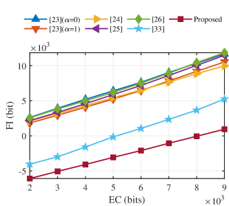
(a) QF=30

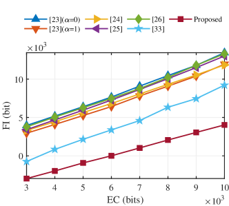
(b) QF=50

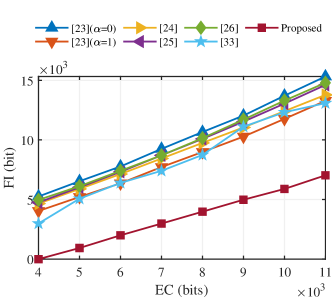
(c) QF=70

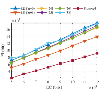
(d) QF=90

Figure 11: Average FI of 200 random images from the BOSSbase image database. The original JPEG images are encoded with the standard Huffman table.

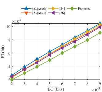
(a) QF=30

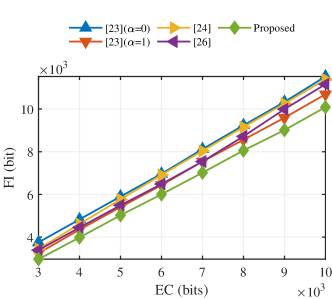
(b) QF=50

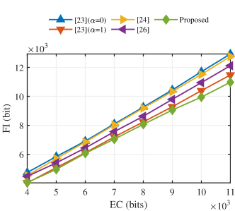
(c) QF=70

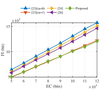
(d) QF=90

Figure 12: Average FI of 200 random images from the BOSSbase image database. The original JPEG images are encoded with the optimized Huffman table.

6.3 Evaluation on image quality

To compare the performance on image quality of marked JPEG images, we tested the MSE of the 200 images from the BOSSbase image database. The results are shown in Fig. 13. As shown in Fig. 13, the MSEs of the proposed method are always equal to zero, which means the marked JPEG images generated by the proposed method maintain an unchanged visual quality compared to the original JPEG images.

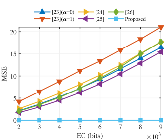
(a) QF=30

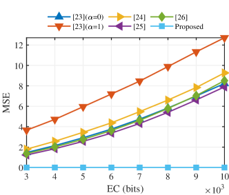
(b) QF=50

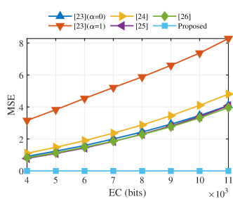
(c) QF=70

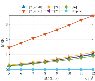
(d) QF=90

Figure 13: Average MSE of 200 images from the BOSSbase image database. The original JPEG images are encoded with the optimized Huffman table.

6.4 Evaluation on complexity

The running times of four test images are listed in Table. 4, where the text in bold indicates the shortest running time of the methods in the same case. It can be observed that the running times of the method [33] are the shortest in most cases. The method [34] is the most time-consuming. Our proposed method is competitive among these high-capacity CM-based methods in terms of runtime.

Table 4: Running time (s) of test images with different QFs using the proposed method and two state-of-the-art CM-based methods [33, 32, 34]. The original JPEG images are encoded with the standard Huffman table.

Image	Method	QF=10	QF=20	QF=30	QF=40	QF=50	QF=60	QF=70	QF=80	QF=90
Baboon	TCSVT2021-I [32]	1.734	1.972	3.423	3.495	4.281	5.804	5.558	5.604	6.299
	Proposed	0.522	0.722	0.942	1.023	1.205	1.299	1.458	1.713	2.514
	TCSVT2021-II [32]	3.192	2.461	3.679	3.779	4.705	6.147	6.048	6.082	7.122
	TDSC2020 [33]	0.438	0.669	0.922	1.057	1.232	1.308	1.624	1.943	2.645
	Proposed	0.543	0.708	0.892	1.026	1.207	1.301	1.467	1.833	2.505
	JVCIR2020 [34]	169.987	220.959	290.210	501.693	544.242	618.708	707.202	458.541	690.555
	Proposed	0.515	0.721	0.853	0.971	1.079	1.192	1.332	1.629	2.226
Boat	TCSVT2021-I [32]	1.378	2.014	2.487	4.396	5.474	5.248	5.441	6.506	7.039
	Proposed	0.418	0.503	0.688	0.667	0.728	0.808	0.899	1.09	1.748
	TCSVT2021-II [32]	1.461	2.015	2.717	4.481	6.074	5.573	6.105	7.674	7.717
	TDSC2020 [33]	0.293	0.449	0.539	0.605	0.684	0.938	0.946	1.204	1.894
	Proposed	0.412	0.600	0.589	0.693	0.725	0.813	0.958	1.221	1.703
	JVCIR2020 [34]	80.529	185.825	297.026	421.591	517.990	666.214	254.186	483.803	916.252
	Proposed	0.399	0.526	0.582	0.652	0.725	0.800	0.905	1.066	1.542
Elaine	TCSVT2021-I [32]	1.313	1.499	1.749	1.758	1.767	1.863	2.377	2.351	3.804
	Proposed	0.385	0.440	0.510	0.577	0.659	0.819	0.784	1.117	1.761
	TCSVT2021-II [32]	1.184	1.809	1.979	1.934	1.919	2.009	2.453	2.572	4.069
	TDSC2020 [33]	0.239	0.332	0.412	0.475	0.632	0.676	0.834	1.081	2.063
	Proposed	0.367	0.521	0.530	0.587	0.708	0.833	0.820	1.179	1.782
	JVCIR2020 [34]	23.740	50.431	82.316	115.965	168.235	180.639	218.327	294.595	451.699
	Proposed	0.344	0.429	0.487	0.542	0.617	0.698	0.798	1.013	1.616
Lena	TCSVT2021-II [32]	1.235	1.546	1.654	2.070	2.216	2.471	2.953	3.891	6.088
	Proposed	0.358	0.425	0.487	0.533	0.636	0.662	0.776	0.886	1.251
	TCSVT2021-II [32]	1.555	1.863	1.871	2.116	2.47	2.513	3.209	4.723	6.541
	TDSC2020 [33]	0.255	0.335	0.469	0.596	0.541	0.611	0.718	0.943	1.435
	Proposed	0.371	0.444	0.488	0.577	0.628	0.665	0.847	0.949	1.349
	JVCIR2020 [34]	67.357	118.483	140.226	240.800	204.149	177.214	222.365	400.918	636.610
	Proposed	0.362	0.438	0.493	0.548	0.605	0.647	0.730	0.880	1.225

The average running time of 200 images from the BOSSbase images database is illustrated in Fig. 14. The original JPEG images in Fig. 14 are encoded with the standard Huffman table. As shown in Fig. 14, the running time of the proposed method is faster than the previous HS-based method but a little slower than the CM-based RDH method proposed by Du $et~{}al.$ [33]. This is because finding a nearly optimal solution using GA is time-consuming.

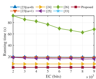
(a) QF=30

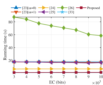
(b) QF=50

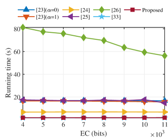
(c) QF=70

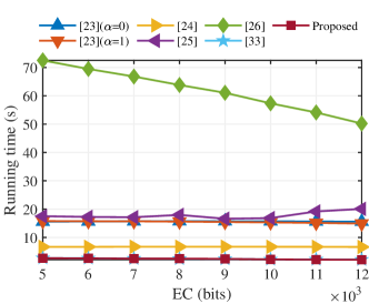
(d) QF=90

Figure 14: Average running time of 200 images from the BOSSbase image database. The original JPEG images are encoded with the standard Huffman table.

7 Conclusion

In this study, we proposed a new CM-based RDH framework to improve the performance of file size preservation and applicability. Compared to the traditional framework of CM-based RDH, the proposed framework adjusts the code-mapping construction step and adds a Huffman table customization step. Using the proposed framework, a new CM-based RDH method can be obtained by designing a specific optimization algorithm. To demonstrate this, we proposed a new CM-based RDH method using a GA to obtain the optimal code-mapping relationship. The experimental results demonstrated that our method achieves impressive file size preservation, visual quality, and time complexity performance. In the future, we will continue to explore the following directions.

1. In our proposed method, solving the optimization algorithm is the key issue. Therefore, more efficient optimization algorithms can be investigated.

2. Recently, reversible data hiding in encrypted images has attracted a considerable attention. The performance of CM-based RDH for encrypted JPEG bitstream should therefore also be investigated.

References

- [1] A. Khan, A. Siddiqa, S. Munib, S. A. Malik, A recent survey of reversible watermarking techniques, Information Sciences 279 (2014) 251–272.
- [2] J. Fridrich, M. Goljan, R. Du, Lossless data embedding—new paradigm in digital watermarking, EURASIP Journal on Advances in Signal Processing 2002 (2) (2002) 986842.
- [3] M. U. Celik, G. Sharma, A. M. Tekalp, E. Saber, Lossless generalized-lsb data embedding, IEEE Transactions on Image Processing 14 (2) (2005) 253–266.
- [4] J. Tian, Reversible data embedding using a difference expansion, IEEE Transactions on Circuits and Systems for Video Technology 13 (8) (2003) 890–896.
- [5] I.-C. Dragoi, D. Coltuc, Local-prediction-based difference expansion reversible watermarking, IEEE Transactions on Image Processing 23 (4) (2014) 1779–1790.
- [6] Z. Ni, Y.-Q. Shi, N. Ansari, W. Su, Reversible data hiding, IEEE Transactions on Circuits and Systems for Video Technology 16 (3) (2006) 354–362.
- [7] X. Li, B. Li, B. Yang, T. Zeng, General framework to histogram-shifting-based reversible data hiding, IEEE Transactions on Image Processing 22 (6) (2013) 2181–2191.
- [8] R. Hu, S. Xiang, Reversible data hiding by using cnn prediction and adaptive embedding, IEEE Transactions on Pattern Analysis and Machine Intelligence (2021) 1–1.
- [9] X. Wang, J. Ding, Q. Pei, A novel reversible image data hiding scheme based on pixel value ordering and dynamic pixel block partition, Information Sciences 310 (2015) 16–35.
- [10] S. Weng, Y. Shi, W. Hong, Y. Yao, Dynamic improved pixel value ordering reversible data hiding, Information Sciences 489 (2019) 136–154.
- [11] R. Kumar, K.-H. Jung, Robust reversible data hiding scheme based on two-layer embedding strategy, Information Sciences 512 (2020) 96–107.
- [12] S. Weng, W. Tan, B. Ou, J.-S. Pan, Reversible data hiding method for multi-histogram point selection based on improved crisscross optimization algorithm, Information Sciences 549 (2021) 13–33.
- [13] J. Fridrich, M. Goljan, R. Du, Lossless data embedding for all image formats, in: Security and Watermarking of Multimedia Contents IV, Vol. 4675, International Society for Optics and Photonics, 2002, pp. 572–584.
- [14] J. Fridrich, M. Goljan, Q. Chen, V. Pathak, Lossless data embedding with file size preservation, in: Security, Steganography, and Watermarking of Multimedia Contents VI, Vol. 5306, International Society for Optics and Photonics, 2004, pp. 354–366.
- [15] J. Lv, S. Li, X. Zhang, A novel auxiliary data construction scheme for reversible data hiding in jpeg images, Multimedia Tools and Applications 77 (14) (2018) 18029–18041.
- [16] S. Ong, K. Wong, Rotational based rewritable data hiding in jpeg, in: 2013 Visual Communications and Image Processing (VCIP), 2013, pp. 1–6.
- [17] J. Long, Z. Yin, J. Lv, X. Zhang, Rotation based reversible data hiding for jpeg images, IETE Technical Review 33 (6) (2016) 607–614.
- [18] G. Xuan, Y. Q. Shi, Z. Ni, P. Chai, X. Cui, X. Tong, Reversible data hiding for jpeg images based on histogram pairs, in: International Conference Image Analysis and Recognition, Springer, 2007, pp. 715–727.
- [19] F. Huang, X. Qu, H. J. Kim, J. Huang, Reversible data hiding in jpeg images, IEEE Transactions on Circuits and Systems for Video Technology 26 (9) (2016) 1610–1621.
- [20] Z. Qian, S. Dai, B. Chen, Reversible data hiding in jpeg images using ordered embedding, KSII Transactions on Internet and Information Systems (TIIS) 11 (2) (2017) 945–958.
- [21] F. T. Wedaj, S. Kim, H. J. Kim, F. Huang, Improved reversible data hiding in jpeg images based on new coefficient selection strategy, EURASIP Journal on Image and Video Processing 2017 (1) (2017) 63.
- [22] D. Hou, H. Wang, W. Zhang, N. Yu, Reversible data hiding in jpeg image based on dct frequency and block selection, Signal Processing 148 (2018) 41–47.
- [23] J. He, J. Chen, S. Tang, Reversible data hiding in jpeg images based on negative influence models, IEEE Transactions on Information Forensics and Security 15 (2020) 2121–2133.
- [24] N. Li, F. Huang, Reversible data hiding for jpeg images based on pairwise nonzero ac coefficient expansion, Signal Processing 171 (2020) 107476.
- [25] Z. Yin, Y. Ji, B. Luo, Reversible data hiding in jpeg images with multi-objective optimization, IEEE Transactions on Circuits and Systems for Video Technology 30 (8) (2020) 2343–2352.
- [26] M. Xiao, X. Li, B. Ma, X. Zhang, Y. Zhao, Efficient reversible data hiding for jpeg images with multiple histograms modification, IEEE Transactions on Circuits and Systems for Video Technology 31 (7) (2021) 2535–2546.
- [27] M. Xiao, X. Li, Y. Zhao, Reversible data hiding for jpeg images based on multiple two-dimensional histograms, IEEE Signal Processing Letters 28 (2021) 1620–1624.
- [28] Z. Qian, X. Zhang, Lossless data hiding in jpeg bitstream, Journal of Systems and Software 85 (2) (2012) 309–313.
- [29] Y. Hu, K. Wang, Z.-M. Lu, An improved vlc-based lossless data hiding scheme for jpeg images, Journal of Systems and Software 86 (8) (2013) 2166–2173.
- [30] Y. Qiu, H. He, Z. Qian, S. Li, X. Zhang, Lossless data hiding in jpeg bitstream using alternative embedding, Journal of Visual Communication and Image Representation 52 (2018) 86–91.
- [31] C. Zhang, B. Ou, D. Tang, An improved vlc mapping method with parameter optimization for reversible data hiding in jpeg bitstream, Multimedia Tools and Applications (2020) 1–18.
- [32] Y. Qiu, Z. Qian, H. He, H. Tian, X. Zhang, Optimized lossless data hiding in jpeg bitstream and relay transfer-based extension, IEEE Transactions on Circuits and Systems for Video Technology 31 (4) (2021) 1380–1394.
- [33] Y. Du, Z. Yin, X. Zhang, High capacity lossless data hiding in jpeg bitstream based on general vlc mapping, IEEE Transactions on Dependable and Secure Computing 19 (2) (2022) 1420–1433.
- [34] C. Zhang, B. Ou, H. Tian, Z. Qin, Reversible data hiding in jpeg bitstream using optimal vlc mapping, Journal of Visual Communication and Image Representation 71 (2020) 102821.
- [35] B. G. Mobasseri, R. J. Berger, M. P. Marcinak, Y. J. NaikRaikar, Data embedding in jpeg bitstream by code mapping, IEEE Transactions on Image Processing 19 (4) (2010) 958–966.
- [36] J. Standard, Information technology-digital compression and coding of continuous-tone still images-requirements and guidelines, International Telecommunication Union. CCITT recommendation 81 (1992) 09.
- [37] The usc-sipi image database, http://sipi.usc.edu/database.
- [38] The bossbase image database, http://agents.fel.cvut.cz/boss.
- [39] The jpeg toolbox, http://dde.binghamton.edu/download/jpeg_toolbox.zip.