Search for glitches of gamma-ray pulsars with deep learning

The pulsar glitches are generally assumed to be an apparent manifestation of the superfluid interior of the neutron stars. Most of them were discovered and extensively studied by continuous monitoring in the radio wavelengths. The Fermi-LAT space telescope has made a revolution uncovering a large population of gamma-ray pulsars. In this paper we suggest to employ these observations for the searches of new glitches. We develop the method capable of detecting step-like frequency change associated with glitches in a sparse gamma-ray data. It is based on the calculations of the weighted $H$-test statistics and glitch identification by a convolutional neural network. The method demonstrates high accuracy on the Monte Carlo set and will be applied for searches of the pulsar glitches in the real gamma-ray data in the future works.

1 Introduction

Pulsars are fast-rotating highly magnetized neutron stars. Rotating at a frequency gradually decreasing over long time due to radiation they rightfully deserve the status of the most precise clocks in the Universe. However, its stability is violated by glitches. Pulsar glitch manifests itself as sudden step-like increase of rotation frequency and its time derivative. Glitch can be characterized by the so-called size — the relative frequency change. Detected glitch sizes vary from very small values $\Delta f/f\sim 10^{-12}$ (McKee, 2016) comparable with timing noise to the largest $\Delta f/f\sim 10^{-5}$ (Espinoza et al., 2011). For example, the Vela pulsar experiences quite large glitches of the size $10^{-6}$ approximately every 1000 days (Cordes et al., 1988; Shannon et al., 2016; Packard et al., 2018), while small frequency changes of the size less than $2\times 10^{-7}$ were demonstrated by the Crab pulsar (Espinoza et al., 2014; Lyne et al., 2015).

Although the first glitch was discovered more than fifty years ago (Radhakrishnan & Manchester, 1969; Reichley & Downs, 1969) (see, e.g. Vivekanand (2017) for a review), the exact origin of these phenomena is still open to debate (Haskell & Melatos,, 2015). Initially, glitches were associated with starquakes (Ruderman, 1969), but then the superfluid model was put forward to explain this phenomena (Packard, 1972). With the discoveries of new glitches we become closer to understanding their nature, which in turn may shed light on the internal structure of the neutron stars (Espinoza et al., 2014).

The radio surveys produced most of the glitch discoveries due to the longest accumulated observation times and the largest number of observed pulsars (see the ATNF pulsar catalog and the JBO online glitch catalog). However, some of the pulsars are radio-quiet, observable only in gamma-ray band with no radio counterpart. Before the launch of the Fermi Gamma-ray Space Telescope with Large Area Telescope (LAT) on board in 2008 (Atwood at al., 2009), there was known only one such object — Geminga (Halpern & Holt, 1992; Bertsch et al., 1992). Now more than 250 LAT sources are identified as gamma-ray pulsars (Abdo at al., 2013) and more than 50 among them are radio quiet. Observations in gamma-rays may provide reach information about glitches and have the potential to search for the difference in their properties of radio-quiet and radio-loud populations.

Large fraction of the LAT-detected gamma-ray pulsars are young and energetic. Recent studies suggest that young pulsars experience glitches more often then the old ones (McKenna & Lyne,, 1990; Lyne et al., 2000; Espinoza et al., 2011). Several glitches of the size of the order of $10^{-5}$ are already discovered simultaneously with the discovery of the pulsars itself via blind searches (Abdo at al., 2009; Saz Parkinson et al., 2010; Pletsch et al., 2012, 2013; Clark et al., 2015). This gives us hope to identify more new glitches in a targeted extensive search in the Fermi-LAT data.

Detection of glitches in the sparse gamma-ray data is computationally challenging. The lack of rigorous criteria to distinguish glitches from other peculiarities at low signal-to-noise ratio compels to search them manually. In this paper we suggest a method which helps to identify glitches automatically. It is based on the computations of the weighted $H$-test statistic (de Jager et al., 1989; de Jager & Busching, 2010) widely used in the blind searches of new gamma-ray pulsars and the glitches analyses (Clark et al., 2017). In order to recognize glitches in the resulting data we suggest to apply the machine learning techniques. It is a modern tool which has already found a lot of applications in a broad range of astrophysical problems (Ball& Brunner, 2010; Baron, 2019) including selection of radio pulsar candidates (Eatough et al., 2010). In this paper using the Monte Carlo data we have show that a convolutional neural network is capable to find pulsar glitches of different sizes with the high accuracy. We plan an extensive applications of the method to the real data in the future works.

2 Method

In this section we describe the method used to detect glitches of the gamma-ray pulsars. We apply it to the Fermi Large Area Telescope data prepared with Fermi Science Tools package according to Sokolova & Rubtsov (2016). The data consist of individual photons recorded between 2008 August 4 (MJD 54682) and 2015 March 3 (MJD 57084) selected from ”SOURCE” class events of the Reprocessed Pass 7 data set by the gtselect tool according to the following criteria. Photons were included if they had energy above $100$ MeV, arrived within $8^{\circ}$ of a target source, with a zenith angle $<100^{\circ}$ and when the LAT’s rocking angle was $<52^{\circ}$.

A source model which includes Fremi-LAT 3FGL sources in a $8^{\circ}$ radius circle, galactic and isotropic diffuse emission components is constructed for each of the pulsar considered in the paper. The model parameters were optimized with unbinned likelihood analysis by the gtlike tool. Next, using the gtsrcprob tool each photon is assigned a weight — probability to be emitted by the source. To search for glitch $40000$ photons with the highest weights were kept for each pulsar.

The glitches search method employs the photon arrival times $t_{i}$ at the solar system barycenter. Position-dependent “barycentering” corrections were calculated by the gtbary tool. These corrections take into account the Earth’s orbital motion which causes Doppler modulation of pulsations and complicates the search for glitches.

At the first step, we combine the data into several time groups which contain photons within the $170$-day time window sliding over the entire data with the $17$-day time step. Working with $6.5$ years of observations we prepared in this way $131$ time groups of the photons. The particular choice of a time-window size and a sliding step were suggested by Pletsch et al. (2013) as a balance between the signal-to-noise ratio and the time resolution of the method. Then the photon arrival times are corrected to compensate for the frequency evolution,

$$\tilde{t}_{i}=t_{i}+\frac{\gamma}{2}(t_{i}-t_{0})^{2}\;,$$ (1)

where $\gamma=\dot{f}/f$ and $t_{0}=286416002$ (MJD 55225) is a reference epoch. Then, the value of $H$ is computed separately for each group of the photons according to the formula

$$H=\max_{1\leq L\leq 20}\left[\sum_{l=1}^{L}\mid\alpha_{l}\mid^{2}-4(L-1)\right]\;,$$ (2)

where $\alpha_{l}$ is a Fourier amplitude of the $l$-th harmonic,

$$\alpha_{l} =\frac{1}{\varkappa}\sum_{i}w_{i}\mathrm{e}^{-2\pi ilf\tilde{t}_{i}}\;,$$

$$\varkappa^{2} =\frac{1}{2}\sum_{i}w_{i}^{2}\;.$$

Fourier exponents in this formula are multiplied by the photon weights $w_{i}$.

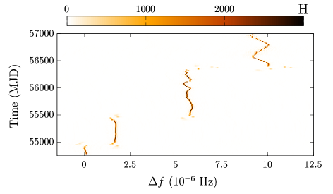
Figure 1: Pulsar glitch analyses for PSR J0007+7303. The weighted $H$-test is calculated according to the equation  (2) using photons within the 170-day time window slided over the entire data set with the 17-day step. For each window scans over $f$ and $\dot{f}$ are done. The maximal value of $H$ over $\dot{f}$ for a given $f$ is shown by color. Vertical axis shows the time midpoint of each time window. Horizontal axis shows the offset in $f$.

Weighted $H$-test staticstics is a powerfull tool to search for weak periodic signals with unknown light curve shape in sparce data. It tests whether photon phases calculated by folding the arrival times $t_{i}$ at a given frequency (and at a given spin-down rate, which enters into equation (1)) are uniformly distributed. Otherwise a periodic signal with spin-parameters $f$ and $\dot{f}$ presents in the data and its significance is given by $H$. Consequently, the correct values of frequency and spin-down rate if unknown a priori can be determined as a maximum of the $H$-test by scanning over it in some range. Performing it separately for each of the time groups of the photons introduced above we obtain data describing the dependence of $H$-test on time, frequency and spin-down rate. In order to reduce the size of the data sample we maximize the $H$-test over $\dot{f}$ at a fixed frequency and time and finally obtain the dependence $H(f,t)$. Exploring these results one can detect an abrupt change of frequency associated with a glitch.

To demonstrate the method we apply it to PSR J0007+7303 in the Fermi-LAT data. The result is presented in Figure 1. The color code represents the weighted $H$-test maximized over the spin-down rate $\dot{f}$. Vertical axis shows the time midpoint of each time group of the photons introduced above. One may see from the figure that frequency position of the maximum $H$ changes abruptly over time revealing three pulsar glitches around 55000 MJD, 55500 MJD and 56400 MJD (for more details see Li et al., 2016).

As one can see from Figure 1, the maximum of the weighted $H$-test between glitches oscillates around a certain frequency. This is due to inaccurate 3FGL sky-coordinates of the source limited by the LAT’s angular resolution to a few arc minutes. As a result, incorrectly taken into account satellite’s motion relative to the source leads to the Doppler modulation of pulsations.

Figure 1 gives an example of the large Vela-type glitches of the size $\Delta f/f\sim 10^{-6}$ clearly visible by the naked eye in the $H$-test data despite the Doppler frequency shift. However, identification of small glitches of the size $\Delta f/f\sim 10^{-8}-10^{-7}$ for the gamma-ray pulsar may become a difficult problem especially if the pulsars are not so bright.

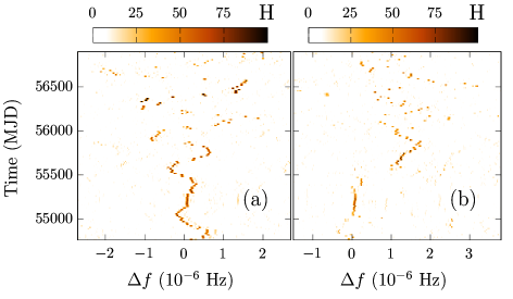
Figure 2: The same as in Figure 1 for: (a) PSR J2030+3641 without glitches during considered epochs and (b) PSR J1422-6138 which experienced glitches at 55310 MJD and 55450 MJD. Computations were performed using coordinates of the sources from the Fermi-LAT 3FGL catalog.

Another source of coherence loss is the poor background rejection when the pulsar is not very bright so that a large number of selected photons were not actually emitted by the pulsar. Figure 2 gives an example of such pulsars: PSR J2030+3641 (see Figure 2a) without glitches during the considered period and PSR J1422-6138 (see Figure 2b) which experienced two glitches (Pletsch et al., 2013). In the computations we used coordinates from the Fermi-LAT 3FGL catalog, therefore the Doppler shift of the frequency presents in the $H$-test data. All that makes glitches of the pulsar shown in Figure 2b hardly distinguishable in the background of other frequency distortions.

More accurate coordinates of the pulsar can be used in the analysis, if they are known from other observations. If not, the loss of phase-coherence can be reduced by refining the sky-location of the source (Yu et al., 2013; Pletsch et al., 2013). However, it enlarges the parameter space of the scan to four-dimensional (sky position, frequency and spin-down rate). A more efficient selection of the photons have to be performed in the case of large background radiation causing frequency distortions in the $H$-test data. As a result, many samples corresponded to each attempt of the scan over coordinates and/or photons selection will be available for the analysis. Visual inspection all of them is rather difficult. Therefore a reliable criterion for automatic glitches search which are able to ”look at” each sample is needed.

3 Convolutional neural network

Efficient glitches identification from other peculiarities in the $H$-test data can be obtained by using the machine learning approach. It provides the ability to “learn” specific patterns corresponding to the pulsar glitch directly from the data, without being explicitly programmed. In the present paper we employ a convolutional neural network (CNN) (Fukushima, 1980; LeCun et al., 1989) — a specialized kind of neural network for processing data that has a grid-like structure. It is widely used in the pattern recognition and image classification problems. In recent years CNNs have seen many applications in physics (Carleo et al., 2019) and astronomy (see, for example, Kim & Brunner,, 2017; Petrillo et al., 2017; Hezaveh et al., 2017; Vernardos & Tsagkatakis, 2019). In this section we will show that CNN is able to detect glitches of gamma-ray pulsars with high accuracy. This gives opportunity for glitches identification in an extensive searches dealing with large amount of data, when it can’t be done manually.

The architecture of the CNN used in this work is presented in Table 1. It was implemented in Python using Keras (Chollet et al., 2015) library with the Tensorflow backend. The network has two components: the feature extraction part and the classification part. The feature extraction part consist of convolution and polling layers which detect specific patterns for pulsars of both kinds. The fully connected layers constitute the classification part. It assign a probabilities that the input data corresponds to glitching (non-glitching) pulsar.

The weighted $H$-test dependence on frequency and time is used for glitches recognition. It is calculated as we have discussed in Section 2. Before being fed to the CNN the data is convolved with a Gaussian function according to the formula

$$\tilde{H}(f,t)=\int_{-\infty}^{\infty}d\tilde{f}\,H(\tilde{f},t)\cdot\frac{1}{\sqrt{2\pi}\delta_{f}}\mathrm{e}^{-\frac{(f-\tilde{f})^{2}}{2\delta_{f}^{2}}}\;.$$ (3)

Search for large glitches generally requires to execute more steps in the scan over frequency. The latter considerably increases the size of the resulting $H$-test array. Thinning in this case will result in loss of high $H$-test values corresponding to some narrow frequency bandwidth. The convolution (3) smooths small scale details spreading the $H$-test values over the scales $f\sim\delta_{f}$. This allows to reduce the size of the array $\tilde{H}$ keeping an average information. The convolution (3) can be calculated at any frequencies within the range covered by the original data. In what follows we compute convolution at $131$ equidistant frequency values for every time group of the photons. As a result we obtain the array of the size $131\times 131$, which is fed to the CNN (see Table 1). The foregoing can be seen in Figure 3, where the original data (see Figure 3a) and the results of convolution (see Figure 3b) are shown.

The CNN predicts whether the input data corresponds to pulsar with glitch or not. The output layer with sigmoid activation function returns a number between $0$ and $1$. If the output is less than $0.5$ we assign the input sample to the pulsars without glitch, otherwise we assign it to the pulsars with glitches.

Table 1: Architecture of the convolutional neural network

No	Layer	Size output
1	Input	131$\times$131$\times$1
2	Conv2D	129$\times$129$\times$16
3	MaxPooling2D	64$\times$64$\times$32
4	Conv2D	62$\times$62$\times$32
5	MaxPooling2D	31$\times$31$\times$32
6	Conv2D	29$\times$29$\times$32
7	MaxPooling2D	14$\times$14$\times$32
8	Conv2D	12$\times$12$\times$32
9	MaxPooling2D	6$\times$6$\times$32
10	Conv2D	4$\times$4$\times$32
11	MaxPooling2D	2$\times$2$\times$32
12	Flatten	128
13	Dropout	128
14	Dense	128
15	Dense	1

The network contains a large number of parameters, tuning which during the training stage requires a large data set. The amount of training data qualifies the ability of the network to identify glitches. Since there are not so many gamma-ray pulsars with glitches known whose can be employed to train the network, we generated them as follows. First of all, we generate randomly the pulsar frequency and spin-down rate within the ranges $1$ Hz $\leq f\leq 10$ Hz and $-10^{-15}\;\text{Hz}\cdot\text{s}^{-1}\leq\dot{f}\leq-10^{-13}\;\text{Hz}\cdot\text{s}^{-1}$ correspondingly. Secondly, we introduce the pulsar light curve as a gaussian peak over a constant background level corresponding to the off-pulse emission. The width of a peak is generated randomly from $0.05$ to $0.45$ of the pulsar period $2\pi/f$. The value of the constant background is generated from $0.1$ to $0.6$ of the peak height. For the pulsars with glitches we also generate the time after which the pulsar frequency and spin-down rate get increments in the ranges $10^{-8}\leq\Delta f/f\leq 10^{-5}$ and $10^{-4}\leq\Delta\dot{f}/\dot{f}\leq 10^{-3}$ correspondingly. Finally, we generate randomly $40000$ photons with unit weights according to this light curve with the barycentric arrival times from 54682 MJD to 57084 MJD which corresponds to $6.5$ years of observations.

The data set of $15000$ pulsars with glitches and $13500$ without glitch was generated. For each of the generated sources the weighed $H$-test data are calculated as discussed in Section 2. The range of the scan over frequency is taken according to the glitch amplitude $\Delta f$ and randomly for pulsars without glitches. Then the convolution (3) is calculated. The results of applying the method to an example of generated pulsar with a glitch are illustrated in Figure 3.

The data are splitted randomly into two subsets: $90\%$ of the data is for the training, $10\%$ — for the validation. To increase the amount of training data we use the augmentation techniques. We randomly crop a region around pre-glitch frequency value from the original array $H(f,t)$ and after convolution with Gaussian function (3) obtain $\tilde{H}(f,t)$. The cross-entropy was used as the loss function assuming the target value of $1$ for all samples of pulsars with glitches and $0$ otherwise. The network was trained during 500 epochs while the overfitting was reduced by including a dropout layer and using $L2$ regularization of the weights in the convolutional layers.

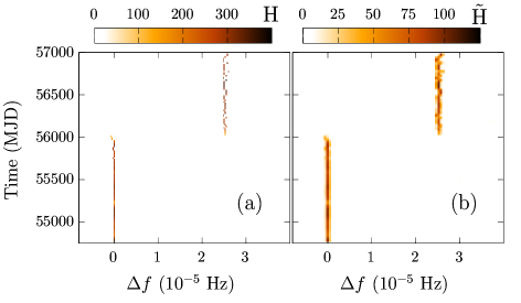
Figure 3: (a) The weighted $H$-test data calculated as we discussed in Section 2 for generated pulsar with glitch and (b) this data after convolution with Gaussian function (3).

In order to test the accuracy of the CNN we generate additional $2500$ pulsars without glitches and $2500$ pulsars with glitches of the amplitude $10^{-10}$ Hz $\leq\Delta f\leq 10^{-5}$ Hz. The network performance on the test data is presented in Figure 4. As one can see from the figure, the CNN demonstrates high accuracy in detection of large glitches. About $98\%$ of pulsars with frequency change $\Delta f\gtrsim 10^{-7}$ Hz were correctly identified. The false positive rate is about $2\%$ over the whole frequency interval of the glitches search. The example of pulsars with glitch correctly identified by the neural network is presented in Figure 5.

The fraction of correctly identified pulsars with glitch gradually decreases with decreasing amplitude of the frequency shift reaching approximately $10\%$ for $\Delta f\lesssim 10^{-8}$ Hz. We checked that an extension of the training data set with pulsars with such small glitches does not improve the accuracy. This means that the method has reached the threshold of sensitivity, which corresponds to a resolution of the 170-day time window $1/\Delta t\simeq 7\times 10^{-8}$ Hz. One can increase the window size, but this does not seem to improve considerably the sensitivity to such small glitches.

The relative number of pulsars with glitch detected by the neural network below the sensitivity threshold was expected to be at the same level as the false positive rate. However, as one can see from Figure 4, this fraction is about $10\%$ which is much higher than $2\%$. The reason is in the non-negligible change in the spin-down rate during glitch which was generated in the range $10^{-4}\leq\Delta\dot{f}/\dot{f}\leq 10^{-3}$. The weighted $H$-test calculated according to the equations (1), (2) was maximized over the spin-down rate leaving dependence on $t$ and $f$. However, some information about change in $\dot{f}$ due to a glitch is likely to remain and is “noticed” by the neural network. In order to test this hypothesis, we generate two sets of 100 pulsars in each with the same glitch amplitude $\Delta f=10^{-10}$ Hz but with different changes of the spin-down rate $\Delta\dot{f}=10^{-20}\;\text{Hz}\cdot\text{s}^{-1}$ and $\Delta\dot{f}=5\times 10^{-17}\;\text{Hz}\cdot\text{s}^{-1}$ respectively. The other parameters are fixed and the same in the each set. The result of applying the neural network to these two sets confirmed the hypothesis: in the set with $\Delta\dot{f}=10^{-20}\;\text{Hz}\cdot\text{s}^{-1}$ two pulsars were correctly identified while in another set the CNN identified 11 samples as pulsars with glitches.

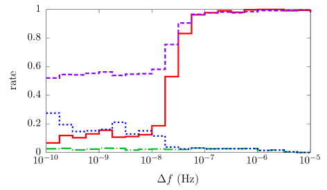
Figure 4: The neural network efficiency of pulsar glitches detection: true positive rate (red solid line) — the proportion of correctly identified pulsars with glitch among all pulsars with glitch of the amplitude $\Delta f$, false positive rate (green dashed-dotted line) — the proportion of erroneously identified as pulsars with glitch among pulsars without glitches in the search for glitches of the amplitude $\Delta f$, accuracy (violet dashed line) — the proportion of correct predictions and false discovery rate (blue dotted line) —  the proportion of erroneously identified as pulsars with glitch among all glitch identifications.

4 Discussion

In this paper we have shown that the convolutional neural network applied to the weighted $H$-test data can be used to detect glitches of the gamma-ray pulsars in an automatic regime. The neural network demonstrates a very high accuracy on the generated data and recognizes pulsars with glitches up to very small amplitudes $\Delta f\sim 10^{-8}\text{Hz}$. It opens up a new possibility to exploit this method in an extensive searches dealing with large amount of data.

To verify that the network is able to recognize glitches in real data we apply it to some gamma-ray pulsars from the Fermi-LAT 3FGL catalog. The neural network correctly identified pulsars with glitch known previously including those presented in Figures 1, 2. We postpone an extensive searches of new glitches with the fine-tuning of coordinates for the future works.

It is worth emphasizing that we have not yet applied the neural network to a large volume of real data, which can turn out to be more complicated for glitches recognition. In the latter case the following improvements of the method are possible. First of all, the scan over source coordinates will be able to recover phase-coherence what will increase the sensitivity of the method. Second, some features of the real data which confuse the network can be replicated in the generation of the training data set. It will allow the network to ”learn” these features and make less mistakes.

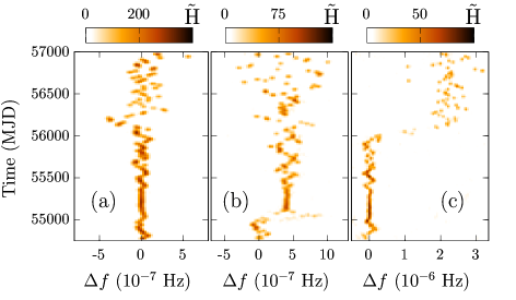
Figure 5: The weighted $H$-test data calculated as we discussed in Section 2 and convolved with Gaussian function (3) for three generated pulsars with glitch: (a) at 56183 MJD with $\Delta f\simeq 4.6\times 10^{-8}$ Hz, (b) at 55045 MJD with $\Delta f\simeq 4.2\times 10^{-7}$ Hz and (c) at 56041 MJD with $\Delta f\simeq 2.2\times 10^{-6}$ Hz