Structure of Spin Correlations in High Temperature SU$(N)$ Quantum Magnets

Abstract

Quantum magnets with a large SU$(N)$ symmetry are a promising playground for the discovery of new forms of exotic quantum matter. Motivated by recent experimental efforts to study SU$(N)$ quantum magnetism in samples of ultracold fermionic alkaline-earth-like atoms in optical lattices, we study here the temperature dependence of spin correlations in the SU$(N)$ Heisenberg spin model in a wide range of temperatures. We uncover a sizeable regime in temperature, starting at $T=\infty$ down to intermediate temperatures and for all $N\geq 2$, in which the correlations have a common spatial structure on a broad range of lattices, with the sign of the correlations alternating from one Manhattan shell to the next, while the amplitude of the correlations is rapidly decreasing with distance. Focussing on the one-dimensional chain and the two-dimensional square and triangular lattice for certain $N$, we discuss the appearance of a disorder and a Lifshitz temperature, separating the commensurate Manhattan high-$T$ regime from a low-$T$ incommensurate regime. We observe that this temperature window is associated to an approximately $N$-independent entropy reduction from the $\ln(N)$ entropy at infinite temperature. Our results are based on high-temperature series arguments and as well as large-scale numerical full diagonalization results of thermodynamic quantities for SU$(3)$ and SU$(4)$ square lattice samples, corresponding to a total Hilbert space of up to $4\times 10^{9}$ states.

I Introduction

More than a decade ago first proposals put forward the use of internal states of ultracold atoms in order to implement various models of SU$(N)$ quantum magnetism and multi-orbital physics Honerkamp and Hofstetter (2004); Cazalilla et al. (2009); Gorshkov et al. (2010). In contrast to ”plain” quantum simulations, where the emulation of a particular condensed matter problem is central to the effort, here the proposals offered a new playground for theory and experiment to explore uncharted territory. The study of SU$(N)$ quantum magnetism started historically as a largely academic endeavour in the context of integrable systems and large-$N$ limits of SU$(2)$ quantum magnetism Sutherland (1975); Affleck and Marston (1988); Read and Sachdev (1989); Marston and Affleck (1989), but in the meantime a large swath of theoretical and numerical work has demonstrated that the field of SU$(N)$ quantum magnetism offers many opportunities for exciting new physics, waiting to be uncovered in experiments Daley (2011); Cazalilla and Rey (2014).

Concerning the experimental AMO platform, it turned out that the alkaline-earth(-like) fermionic atoms ⁸⁷Sr DeSalvo et al. (2010); Tey et al. (2010); Stellmer et al. (2011, ); Zhang et al. (2014); Qi et al. (2019); Sonderhouse et al. (2020); Bataille et al. (2020) and ¹⁷³Yb Fukuhara et al. (2007); Taie et al. (2010); Sugawa et al. (2011); Pagano et al. (2014); He et al. (2020) are well suited for this line of research. On the road towards SU$(N)$ quantum magnetism of localized moments on a lattice, the realization of a Mott insulating state of ¹⁷³Yb atoms formed an important milestone Taie et al. (2012); Hofrichter et al. (2016), paralleling the earlier achievements of SU$(2)$ Mott insulators Jördens et al. (2008); Schneider et al. (2008). The realm of SU$(2)$ magnetism has seen tremendous experimental progress with the advent of the real-space resolution of spin correlations using quantum gas microscopes and other probes Greif et al. (2013); Parsons et al. (2016); Boll et al. (2016); Cheuk et al. (2016); Brown, Peter T. and Mitra, Debayan and Guardado-Sanchez, Elmer and Schauß, Peter and Kondov, Stanimir S. and Khatami, Ehsan and Paiva, Thereza and Trivedi, Nandini and Huse, David A. and Bakr, Waseem S. (2017); Mazurenko et al. (2017); Hart et al. (2015). For ¹⁷³Yb first promising experimental results for nearest neighbor spin correlations in SU$(4)$ and SU$(6)$ Mott insulators were reported recently Ozawa et al. (2018); Takahashi (2018, 2020), and efforts towards quantum gas microscopes for Sr or Yb atoms are on their way Miranda et al. (2015, 2017); Knottnerus et al. (2020); Okuno et al. (2020).

The original proposals and the subsequent experimental work motivated a broad range of theoretical and computational works on various aspects of SU$(N)$ quantum magnets Frischmuth et al. (1999); Manmana et al. (2011); Messio and Mila (2012); Bonnes et al. (2012); Yip et al. (2014); Decamp et al. (2016); Huang et al. (2019); Nonne et al. (2013); Rachel et al. (2009); Dufour et al. (2015); Capponi et al. (2016); Tanimoto and Totsuka (2015); Suzuki et al. (2015); Okubo et al. (2015); Motoyama and Todo (2018); Gauthé et al. (2020); Sotnikov and Hofstetter (2014); Sotnikov (2015); Yanatori and Koga (2016); Golubeva et al. (2017); Kanász-Nagy et al. (2017); Assaad (2005); Hazzard et al. (2012); Cai et al. (2013); Zhou et al. (2014); Wang et al. (2014); Lee et al. (2018); Tamura and Katsura (2019); Chung and Corboz (2019); Choudhury et al. (2020); Fukushima and Kuramoto (2002); Fukushima (2003, 2005); Nataf and Mila (2014); Nataf et al. (2016a). A significant effort was put into understanding the ground state ($T=0$) phase diagrams of quantum spin models in the fundamental representation of SU$(N)$ van den Bossche et al. (2000, 2001); Penc et al. (2003); Läuchli et al. (2006); Hermele et al. (2009); Tóth et al. (2010); *Toth2012; Corboz et al. (2011); Hermele and Gurarie (2011); Corboz et al. (2012a, b); Bauer et al. (2012); Corboz et al. (2013); Song and Hermele (2013); Capponi et al. (2016); Nataf et al. (2016a, b); Weichselbaum et al. (2018); Keselman et al. (2019); Boos et al. (2020).

The experiments for Mott insulators of ¹⁷³Yb Taie et al. (2012); Hofrichter et al. (2016) operate currently in a temperature $(T)$ or entropy $(S)$ regime, which is low enough to freeze out the charge fluctuations at the repulsion energy $U$, therefore justifying the Mott insulating regime. However the thermal entropy per particle is still substantial, so that one likely operates at effective temperatures above or around the magnetic exchange scale $J$.

In this manuscript we address the structure and temperature dependence of real-space and momentum-space spin correlations in this particular temperature or entropy regime. We find an underlying common structure of correlations in real-space for all $N$ in SU$(N)$ and across many lattices. We also find that many aspects of the thermodynamics in this regime are to a large extent $N$-independent.

II Model

An appropriate starting point to describe the systems of interest is a single-band, SU$(N)$-symmetric, fermionic Hubbard model, which models ¹⁷³Yb or ⁸⁷Sr atoms (in the electronic ${}^{1}S_{0}$ ground state) confined to an optical lattice .

$${\cal H}_{\mathrm{Hubbard}} = -t\ \sum_{\langle i,j\rangle,\alpha}\Bigl{(}c^{\dagger}_{i,\alpha}c^{\phantom{\dagger}}_{j\alpha}+\mathrm{h.c.}\Bigr{)}$$

$$+\ \frac{U}{2}\sum_{i}n_{i}(n_{i}-1)\ .$$

Here $t$ denotes the tunneling amplitude for nearest neighbor bonds on the lattice and $U>0$ parametrizes the repulsive onsite interaction strength. $c^{\dagger}_{i,\alpha}$ ($c^{\phantom{\dagger}}_{i\alpha}$) are the creation (annihilation) operators of fermions with internal state $\alpha\in\{1,\ldots,N\}$ on lattice site $i$. The operator $n_{i}\equiv\sum_{\alpha}n_{i,\alpha}=\sum_{\alpha}c^{\dagger}_{i,\alpha}$ $c^{\phantom{\dagger}}_{i\alpha}$ determines the total number of fermions on site $i$.

While the general phase diagram of this model is to a large extent unknown, and the charting thereof constitutes one of the goals of the experimental investigations, it is clear that at integer fillings, in the limit of strong repulsive interactions $U\gg|t|$ and low temperature $T\ll U$, Mott insulating phases do occur, where charge fluctuations are suppressed, and the system is thus insulating, i.e. charge transport is inhibited. In this limit the description of the system can be simplified by projecting out the local occupancies away from the considered integer filling and therefore adopting an SU$(N)$ symmetric effective spin model. Depending on the integer filling $\langle n_{i}\rangle=n$, the spin model is formulated with local spins in the $n$-box antisymmetric irreducible representation of SU$(N)$. The Heisenberg spin model then reads

$${\cal H}_{\mathrm{HB}}=J\sum_{\langle i,j\rangle,A}S^{A}_{i}S^{A}_{j}\text{ ,}$$ (2)

with the antiferromagnetic coupling $J=4t^{2}/U>0$ at leading order in $t/U$ . The sum $A$ extends over the $N^{2}-1$ generators of SU$(N)$. The dimension of the spin operators depends on the irreducible representation considered, and we will now focus exclusively on the case of unit filling $n=1$, corresponding to the fundamental irreducible representation of SU$(N)$ (Young tableau: ${\tiny\yng(1)}$ ) of dimension $N$. In this particular case the spin interaction can also be rewritten exactly as a sum of two-site transposition operators:

$${\cal H}_{\mathrm{HB}}=J\sum_{\langle i,j\rangle}\tfrac{1}{2}(P_{ij}-\tfrac{1}{N})\text{ ,}$$ (3)

with $P_{ij}=\sum_{\alpha,\beta}|\alpha_{i},\beta_{j}\rangle\langle\beta_{i},\alpha_{j}|$, i.e. a two site permutation operator with $\alpha,\beta\in\{1,...,N\}$. Some parts of the recent literature on quantum spin models in the fundamental representation are working with this permutation formulation. In order to allow for a simple comparison to the established correlations and temperature scales for SU$(2)$ we however continue our discussion with the Heisenberg Hamiltonian in the spin operator convention Eq. (2). We discuss the relation between different observables quantifying spin correlations in App. A.

As mentioned in the introduction, our goal is to explore and characterize the structure of spin correlations in a temperature regime where the charge fluctuations can be neglected, i.e. at $T\ll U$. This is an experimentally relevant regime, as some of the currently reported experiments operate at entropies per particle around or somewhat below $\ln N$ Hofrichter et al. (2016) in the Mott regime. In the spin language this corresponds to temperature ranges from $T/J\sim 1$ to $T/J=\infty$. While spin correlations of one-dimensional spin chains have been studied at finite temperature in the past Frischmuth et al. (1999); Fukushima and Kuramoto (2002); Messio and Mila (2012); Bonnes et al. (2012), there is a scarce number of works Fukushima (2005) addressing SU$(N)$ spin correlations at finite temperature in higher dimensions.

Our work is based on simple high-temperature series considerations Oitmaa et al. (2006), complete numerical exact diagonalization (ED) of periodic finite size clusters using a basis of SU$(N)$ Young tableaux Nataf and Mila (2014) and numerical linked cluster expansion Rigol et al. (2007) results (also in the SU$(N)$ Young tableaux basis), and aims to explore the structure and temperature behaviour of spin correlations in the currently experimentally accessible temperature or entropy regime in SU$(N)$ Mott insulators across a variety of (mostly two-dimensional) lattices.

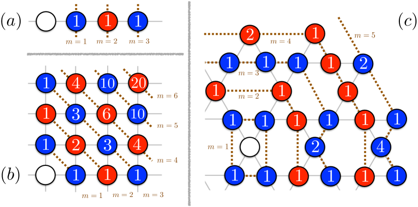
Figure 1: Manhattan physics for SU$(N)$ magnets. Qualitative real-space two-site correlation pattern in the high-temperature regime $J{\ll}T{\ll}U$ of the SU$(N)$ Heisenberg model on different geometries: (a) one dimensional chain, (b) square lattice and (c) kagome lattice. Blue (red) denotes a negative (positive) correlation with the reference site (empty circle symbol). The sign of the correlator only depends on the Manhattan distance $m$ to the reference site. The dotted brown line connects equidistant sites from the reference site and forms Manhattan-shells denoted by $m$, i.e. nearest neighbors to the reference site are found in the first shell $m=1$, then at distance two $m=2$ the second shell, etc.. The prefactor $g_{\mathrm{paths}}(\mathbf{r})$ of the corresponding correlator is indicated at the lattice sites. $g_{\mathrm{paths}}(\mathbf{r})$ counts the number of possible paths connecting the two sites with $m$ Manhattan distance steps (using only nearest neighbor bonds).

III Spin Correlations at high Temperature

We start with a simple, but insightful, high-temperature series consideration. We are interested in the following temperature dependent spin correlations at distance $\mathbf{r}\neq\mathbf{0}$ :

$$C_{\mathrm{spin}}(T,\mathbf{r})=\operatorname{Tr}\left[\hat{\rho}(T)\ \sum_{A}S^{A}_{\mathbf{0}}S^{A}_{\mathbf{r}}\right]$$ (4)

The density matrix

$$\hat{\rho}(T)=\frac{\exp(-\mathcal{H}_{\mathrm{HB}}/T)}{Z(T)}$$ (5)

is the standard normalized canonical Gibbs density matrix (we set $k_{B}=1$), where $Z(T)=\operatorname{Tr}[\exp(-\mathcal{H}_{\mathrm{HB}}/T)]$ denotes the partition function. We assume a translation invariant situation and choose the reference site at the origin $\mathbf{0}$. For other observables suitable to capture SU$(N)$ spin correlations and their relation, please refer to App. A.

At infinite temperature $(T/J=\infty)$ in the spin model (2) all spin correlations as defined above vanish (c.f. App. A), irrespective of the value of $N$.

Let us now discuss the leading order behaviour in $\beta J=J/T$ for a correlation at distance $\mathbf{r}$ for a general lattice made of nearest neighbour bonds of the same strength. Standard linked cluster arguments for high-temperature series Oitmaa et al. (2006) imply that the correlator at distance $\mathbf{r}$ starts at an order $k$ in $(\beta J)$ which is directly linked to the Manhattan distance $m$ between the origin $\mathbf{0}$ and site $\mathbf{r}$. In Fig. 1 we indicate the Manhattan distance $m$ between the reference site and a few shells of sites on (a) the linear chain, (b) the square lattice and (c) the kagome lattice for illustration. The structure on other lattices can be derived accordingly. As discussed below an additional element of the leading order expression concerns the number of shortest paths $g_{\mathrm{paths}}(\mathbf{r})$, measured in the Manhattan metric, which link the origin to the site of interest. These numbers $g_{\mathrm{paths}}(\mathbf{r})$ are marked in the site circles in Fig. 1.

The considerations so far are independent of the actual Hamiltonian, as long as it consists only of nearest neighbor bonds on the lattice. There are also interesting connections to the short-time expansion of correlations when starting from an uncorrelated product state, as recently discussed and experimentally demonstrated in a Rydberg quantum magnetism experiment on square and the triangular lattices Lienhard et al. (2018).

For our Hamiltonian at hand, when written in the permutation formulation (3), it is possible to explicitly calculate the coefficient of the leading order high-temperature expression symbolically for all $N$ Fukushima and Kuramoto (2002); Fukushima (2003) for the first few orders $k\leq 12$. Given the simple structure of the terms we conjecture that the expression holds for all $k$. Based on these results we are now in a position to present the leading order high-temperature expression for general $N$ on any lattice in any dimension, as long as the Hamiltonian (2) only contains nearest-neighour bonds of equal strength:

$$C_{\mathrm{spin}}(T,\mathbf{r}) = \frac{g_{\mathrm{paths}}(\mathbf{r})}{2}(-K)^{m}\left(\frac{1}{N^{m-1}}-\frac{1}{N^{m+1}}\right)$$ (6)

$$+O(K^{m+1}),$$

where $K=\beta J/2$, and $m$ is the Manhattan distance between sites $\mathbf{0}$ and $\mathbf{r}$ on the considered lattice, while $g_{\mathrm{paths}}(\mathbf{r})$ counts the number paths between the two sites of length $m$, measured in the Manhattan metric.

This is a central result of our work. The expression (6) allows us to predict both the real-space structure of the correlations, and their relative $N$ dependence in the high-temperature regime of Hamiltonian (2), within the limits of its applicability, to be discussed below.

As one can see from the term $(-K)^{m}$, the spin correlations are alternating in sign from one Manhattan shell to the next, starting with the nearest-neighbour correlations being negative, i.e. antiferromagnetic, as expected for an antiferromagnetic spin Hamiltonian. This feature has been noticed before in earlier work on linear chains Fukushima and Kuramoto (2002) and the cubic lattice Fukushima (2005). Furthermore sites within the same Manhattan shell $m$ are more correlated by a factor $g_{\mathrm{paths}}(\mathbf{r})$, when multiple paths link the two considered sites. These enhancement factors are displayed in the circles in Fig. 1.

The dependence on $N$ in SU$(N)$ is also remarkable. For $m=1$, i.e. nearest neighbours, the correlations are proportional to $(1-1/N^{2})$, indicating that the correlations are actually increasing with $N$ and converging to a constant value at large $N$ (for a given $K$). This is also an important feature, and its thermodynamic implications will be discussed further in Sec. V. For more distant sites with $m>1$ the correlations are proportional to $(1/N^{m-1}-1/N^{m+1})$ indicating that the correlations decrease rapidly in magnitude with $m$ and converge towards zero as $N$ grows, and even more strongly so for larger $m$.

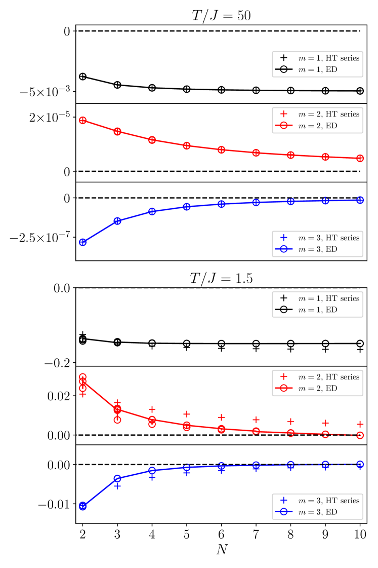
Figure 2: Real space spin correlations on the square lattice for two different temperatures: $T/J=50$ for the upper panel (with distances $m=1,2,3$) and $T/J=1.5$ for the lower panel (for the same distances). The empty circles denote numerical exact diagonalization results while the crosses correspond to the leading order high-temperature series result presented in Eq. (6).

As a first step towards addressing the range of applicability of the leading-order high temperature series argument just developed, we display in Fig. 2 numerical exact diagonalization results for several finite-size square lattice clusters at different temperatures $T/J$ and distances $m$ as a function of $N\in\{2,\ldots,10\}$ . In the upper three panels of Fig. 2 we start at a rather high temperature of $T/J=50$. We show three panels, one for each $m=1$ (black), $2$ (red), and $3$ (blue). At this temperature, for the distances shown, the agreement between the high-temperature series expansion result (6) (crosses) and the ED results (circles) is very good. One can also clearly see the rapid decay of the correlations with the distance $m$ and, for $m>1$, with $N$. The values of the correlations themselves are extremely small at this temperature. For the substantially lower temperature $T/J=1.5$ the lower three panels highlight how the quantitative agreement between the result (6) and the numerics starts to deteriorate, however the qualitative trends remain unaltered and even a semi-quantitative agreement is visible. These numerical results provide strong evidence that the Manhattan picture introduced here prevails for a sizeable range in temperature and spatial extent for a broad range of values of $N$.

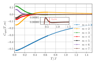
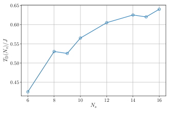
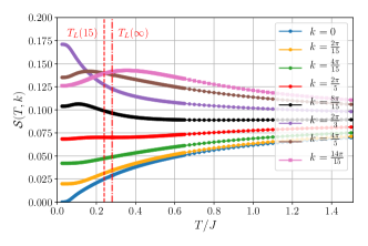
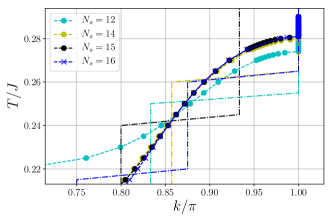
Figure 3: Temperature dependence of spin correlations in the one-dimensional SU$(3)$ Heisenberg model: (a) Real-space spin-spin correlations $C_{\mathrm{spin}}(T,m)$ between sites at distance $m$ as a function of temperature $T/J$ for a $N_{s}=15$ sites chain. The inset resolves the sign change occurring as a function of $T/J$ for the $m=7$ correlator. (b) Disorder temperature $T_{D}(N_{s})/J$ as a function of system size $N_{s}$. (c) Static structure factor as a function of temperature $T/J$. The vertical red dotted and dashed dotted lines indicate the finite size bifurcation temperature $T_{L}(N_{s}=15)/J\approx 0.24$ (on the periodic $15$-site chain) and the estimated infinite system size Lifshitz temperature $T_{L}(\infty)/J=0.281(5)$. (d) Evolution of the peak location $k/\pi$ of the structure factor as a function of temperature $T/J$ for different chain lengths $N_{s}$. Dashed dotted lines are finite-size ED data and display jumps when the peaks transition from one finite size momentum to another, using a temperature grid of $\Delta T/J=0.005$. Solid lines with symbols correspond to results obtained using the continuous structure factor ansatz of App. C.

IV Disorder temperatures and Lifshitz transitions

In this section we study in more detail for which distances and temperatures the Manhattan picture starts to break down. The ground state physics of the spin Hamiltonian (2) has been explored for many values of $N$ and lattice geometries over the last decades, see e.g. Refs. Sutherland (1975); van den Bossche et al. (2000, 2001); Penc et al. (2003); Läuchli et al. (2006); Hermele et al. (2009); Tóth et al. (2010); *Toth2012; Corboz et al. (2011); Hermele and Gurarie (2011); Corboz et al. (2012a, b); Bauer et al. (2012); Corboz et al. (2013); Song and Hermele (2013); Capponi et al. (2016); Nataf et al. (2016a, b); Weichselbaum et al. (2018); Keselman et al. (2019); Boos et al. (2020), and in most cases the structure of the ground states differs qualitatively from the Manhattan picture advocated in the previous section. Based on the current understanding, we expect only bipartite lattices with $N=2$ to show a common sign structure of correlations from high to low temperatures. In all other cases we have to assume the Manhattan picture to break down at some temperature in one way or the other. In the following we discuss some scenarios on how this breakdown might occur.

We start a few general considerations and discuss the notions of a disorder temperature, a Lifshitz temperature, and a thermal first order phase transition. We then apply these notions to discuss the well understood one-dimensional chain case for $N=3$ first, and then switch to two-dimensional square lattices, where we focus on $N=3$ and $N=4$. We close this section with a brief analysis of the $N=3$ model on the triangular lattice.

IV.0.1 Disorder temperature $T_{D}(N_{s})$

For each distance, the high-temperature expansion starts with the expression given by Eq. (6). We have however no detailed understanding of the form of the coefficient of the next order contribution in the high-temperature expansion. Such an analysis would require a fully fledged series expansion machinery as in Refs. Fukushima and Kuramoto (2002); Fukushima (2003, 2005), which is however not the goal of the present work. In order to quantify the deviation we follow an idea put forward in the context of commensurate-incommensurate transitions of short-range ordered magnetic systems Stephenson (1969, 1970); Schollwöck et al. (1996). In such systems, the transition from a commensurate regime to an incommensurate regime can be detected in real-space or momentum space. In real space, one diagnostic is to determine the transition point (as a function of a parameter, such as a coupling in the Hamiltonian, or in our case the temperature $T/J$) by locating the first sign change in a correlator at any distance deviating from the commensurate structure. In our case the commensurate region is the one with the alternating Manhattan shell structure. The parameter location is called a disorder point. Since in our case at hand we are interested in the temperature dependence, we call this system size dependent temperature, the disorder temperature $T_{D}(N_{s})$. Note that this temperature does not necessarily indicate a thermodynamic phase transition, just a change in the nature of short range correlations.

IV.0.2 Lifshitz temperature $T_{L}(N_{s})$

Another diagnostic to track the change from commensurate to incommensurate behaviour is to determine when the peak in the corresponding structure factor is moving away from a commensurate location. The structure factor is defined as the Fourier transform of the real-space correlations:

$$\mathcal{S}(T,\mathbf{k})=\frac{N^{2}-1}{2N}+\sum_{\mathbf{r}\neq\mathbf{0}}\left(C_{\mathrm{spin}}(T,\mathbf{r})\ \exp[{i\mathbf{k}\cdot\mathbf{r}}]\right).$$ (7)

In two of the specific geometries discussed below, the linear chain and the square lattice, the Manhattan shell structure of correlations in real space leads to a peak in the structure factor at momentum $\pi$ or $(\pi,\pi$) respectively. We can then track the structure factor as a function of temperature $T/J$ and detect the first temperature, coming from $T/J=\infty$, where the location of the maximum starts to deviate continuously from $\pi$ or $(\pi,\pi)$, as in a bifurcation transition. This (possibly finite-size dependent) temperature is called the Lifshitz temperature $T_{L}(N_{s})$. In analogy to the disorder temperature, the Lifshitz temperature is not necessarily an indication for a thermodynamic phase transition.

IV.0.3 First order phase transition

In dimensions higher than one, another distinct possibility is that the Manhattan regime is separated from one or several low-temperature regimes by a genuine thermal first order phase transition. In such a scenario correlations in real space would change discontinously for many distances, and the structure factor location is also expected to jump discontinously away from the commensurate position.

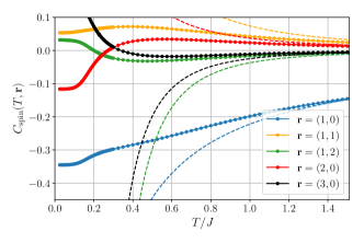
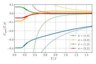
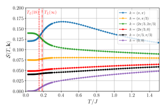
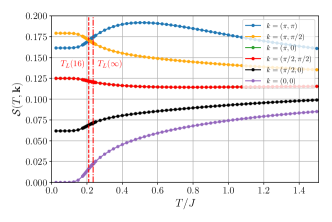
Figure 4: Temperature dependence of spin correlations in the two-dimensional square lattice SU$(3)$ and SU$(4)$ Heisenberg model: Full ED spin correlation results for the largest accessible clusters for SU($3$) ($N_{s}=18$) and SU($4$) ($N_{s}=16$). (a) and (b) shows the correlation functions $C_{\mathrm{spin}}(T,\mathbf{r})$ with a fixed reference site $0$ for $N=3$, $N_{s}=18$ and $N=4$, $N_{s}=16$, respectively. Leading order high-temperature expansion results [Eq. (6)] are illustrated as dashed lines. (c) and (d) shows the corresponding structure factor $\mathcal{S}(T,\mathbf{k})$. The vertical red dashed and dashed dotted lines indicate the finite size bifurcation temperature $T_{L}(N_{s}{=}18)/J=0.150(5)$ [$T_{L}(N_{s}{=}16)/J=0.210(5)$] and the estimated infinite system size Lifshitz temperature $T_{L}(\infty)/J=0.180(5)$ [$T_{L}(\infty)/J=0.230(5)$ for SU$(4)$], obtained by the continuous structure factor ansatz.

IV.1 One-dimensional $N=3$ chain

As a warm-up application of these notions we discuss the SU$(3)$ spin chain. The disorder temperature has not been discussed yet for SU$(N)$ Heisenberg chains, to the best of our knowledge. The Lifshitz temperature has been discussed under a different name in Ref. Fukushima and Kuramoto (2002).

For all $N$ the Manhattan regime of one-dimensional chains is characterized by alternating correlations as shown in Fig. 1(a) and a maximum in the structure factor at wave vector $k=\pi$. We proceed by analyzing finite-size complete ED results for SU$(3)$ chains up to $N_{s}=15$. For each finite system size at high enough temperature the sign (and approximate values) of the correlations are given by Eq. (6). In Fig. 3(a) we display the real-space correlations as a function of the temperature $T/J$ for a system size $N_{s}=15$. For high temperatures all real-space correlators indeed exhibit the sign predicted by the Manhattan regime, i.e. the correlations alternate from one site to the next. However at $T/J=T_{D}(N_{s}=15)/J\approx 0.62J$ the first correlator changes its sign, see the inset for $m=7$ in Fig. 3(a). At even lower temperatures other correlators change their sign, e.g. at distance $m=2$ the correlation changes sign around $T/J\approx 0.3$. In Fig. 3(b) we plot the system size dependence of $T_{D}(N_{s})/J$ for the SU$(3)$ linear chain. We observe a substantial drift of these disorder temperatures towards higher values as $N_{s}$ increases . It is not clear to us whether this disorder temperature will drift to infinite temperature as the system size increases, or wether it will converge to a finite value $T_{D}(\infty)$. Assuming the scenario of a finite disorder temperature, a linear extrapolation in $1/N_{s}$ yields $T_{D}(\infty)/J\approx 0.74(2)$. Irrespective of this uncertainty, we interpret our observations as an indication that the real-space extent and the temperature extent of our proposed Manhattan structured correlation regime is substantial enough that it will be able to be explored in near-term experiments measuring spin correlations beyond nearest neighbour distances.

Next we consider the correlations in momentum space by investigating the structure factor $\mathcal{S}(T,\mathbf{k})$ of the SU$(3)$ Heisenberg chain. At infinite temperature the structure factor is flat throughout the Brillouin zone. At high but finite temperature the structure factor shows a broad peak at momentum $k=\pi$ for even $N_{s}$ or at $k=\pi\pm\pi/N_{s}$ for odd $N_{s}$ (see also Ref. Fukushima and Kuramoto (2002); Bonnes et al. (2012); Messio and Mila (2012)). This is shown in Fig. 3(c). For $N_{s}=15$ we see a shift of the location of the maximum from $k=14\pi/15$ to $k=4\pi/5$ at the finite size Lifshitz temperature $T_{L}(15)/J\approx 0.24$. This is followed by a further change from $k=4\pi/5$ to $k=2\pi/3$ around $T/J\approx 0.15$. The location of the low-temperature peak is in agreement with the known ground state physics of SU$(N)$ Heisenberg chains, which display algebraically decaying spin correlations oscillating with wave vectors which are multiples of $|k|=2\pi/N$ Sutherland (1975); Fukushima and Kuramoto (2002); Bonnes et al. (2012); Messio and Mila (2012). In Fig. 3(d) we analyze the finite size dependence of Lifshitz temperature $T_{L}(N_{s})$ using an expansion of the structure factor around $k=\pi$ discussed in App. C. The analysis leads to a Lifshitz temperature of $T_{L}(\infty)/J=0.281(5)$ for the one-dimensional SU$(3)$ Heisenberg chain. In Ref. Fukushima and Kuramoto (2002) the Lifshitz temperature was discussed for $N=4$ and $N=20$ and a Lifshitz temperature of about $T/J\approx 0.25$ in our units was found, lending support for an approximatively constant Lifshitz temperature for $N\geq 3$. In Ref. Messio and Mila (2012) it was noticed on the other hand that the entropy per spin corresponding to these Lifshitz temperatures is increasing with $N$. We will come back to this observation in Sec. V.

Let us summarize for the $N=3$ Heisenberg chain that coming from high temperature, the first signal in temperature is likely the disorder temperature $T_{D}/J\lesssim 0.73$ (depending on distance or system size), where the sign structure in real space starts to show defects with respect to the Manhattan structure. At a lower temperature $T_{L}/J\sim 0.28$ the peak in the structure factor starts to move away from the commensurate $\pi$ location. So real-space correlations are indeed a valuable new probe to investigate SU$(N)$ magnetism, as they are able to detect deviations from the Manhattan regime at higher $T/J$ than momentum space probes.

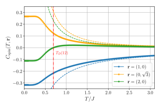
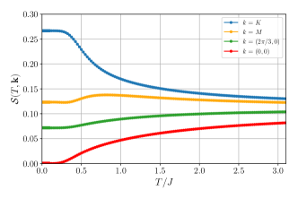
Figure 5: Temperature dependence of spin correlations in the two-dimensional triangular lattice SU$(3)$ Heisenberg model: Full ED spin correlation results for $N_{s}=12$. (a) shows the correlation functions $C_{\mathrm{spin}}(T,\mathbf{r})$ with a fixed reference site $0$. Leading order high-temperature expansion results [Eq. (6)] are illustrated as dashed lines. The vertical red dashed dotted line indicates a disorder temperature $T_{D}(N_{s}=12)/J\approx 0.69$, where the distance $2$ correlator changes sign. (b) shows the corresponding structure factor $\mathcal{S}(T,\mathbf{k})$.

IV.2 Square Lattices: $N=3$ and $N=4$

The Manhattan regime for the square lattice for all $N$ exhibits real-space correlations according to Fig. 1(b), while in momentum space the structure factor peaks at $(\pi,\pi)$. On the other hand the predicted ground state physics scenarios differ starkly among the studied cases of $N$. The SU$(2)$ case is a well-known and its ground state is Néel ordered. The correlations are expected to retain their sign structure from high temperatures down to $T/J=0$, while the structure factor remains peaked at $(\pi,\pi)$ for all $T/J<\infty$.

The SU$(3)$ Heisenberg model on the square lattice also shows long-range spin order Tóth et al. (2010); Bauer et al. (2012), with an ordering wave vector $\pm(2\pi/3,2\pi/3)$ or $\pm(-2\pi/3,2\pi/3)$. The two distinct orientations differ in their sign of the spin correlations across the diagonal of a square plaquette. This difference can be elevated to an Ising order parameter which could order at finite temperature due to its discrete nature, despite the true long range order of the spin correlations being inhibited at finite temperature due to the Hohenberg-Mermin-Wagner theorem Mermin and Wagner (1966); Hohenberg (1967). This scenario is similar to those put forward for frustrated SU$(2)$ systems Chandra et al. (1990); Weber et al. (2003), and being actively discussed in the context of nematic ordering in the pnictide superconductor materials Fang et al. (2008); Xu et al. (2008).

The ground state of the SU$(4)$ square lattice Heisenberg model is predicted to exhibit an even more involved spatial pattern of SU$(4)$ symmetry breaking Corboz et al. (2011). Here it is also conceivable that the dimerization pattern orders at finite temperature, before true long-range order for the spins occurs at $T=0$.

In both the SU$(3)$ and the SU$(4)$ cases predicted the low-temperature regime is distinct from the Manhattan regime expected at high temperature. We discuss in the following complete ED simulations on a $N_{s}=18$ square cluster for SU$(3)$ and a $N_{s}=4\times 4=16$ sites cluster for SU$(4)$ and study the behaviour of real-space correlations and structure factors as a function of temperature $T/J$. These complete numerical diagonalizations have been performed by adopting the SU$(N)$ Young tableaux basis Nataf and Mila (2014), combined with large-scale SCALAPACK SCA highly parallel diagonalization routines. The largest block to be diagonalized numerically had a dimension of almost 800’000. A microcanonical view on the SU$(3)$ data is discussed in App. B.

We start the discussion of the results for the real-space correlations of the two cases in Fig. 4(a) and (b) for SU$(3)$ and SU$(4)$ respectively. The lines including the circle symbols display the ED results evaluated at the corresponding temperatures. The dashed lines on the other hand display the leading order behaviour Eq. (6) of the Manhattan regime. The high-temperature sign structure in the ED data in both cases is in perfect agreement with our Manhattan regime prediction and extends down to an intermediate temperature of $T_{D}/J\approx 0.325$ for SU($3$) where the distance-$(3,0)$ correlator turns from negative to positive. For SU($4$) the distance-$(2,2)$ correlator changes sign at $T_{D}/J\approx 0.575$, which is almost twice as high as in the $N=3$ case. In both cases the deviation from the Manhattan picture occurs at the largest possible distance on the considered cluster, which is analogous to the one dimensional chain discussed above. It is noteworthy that the correlations beyond the nearest neighbor distance remain quite small in the $N=4$ case compared to the $N=3$ case, even down to rather low temperatures.

In Fig. 4(c) and (d) we show the structure factor for various distinct wave vectors as a function of $T/J$ for SU$(3)$ and SU$(4)$ respectively. As expected we observe a maximum at $(\pi,\pi)$ in the high temperature regime. At low temperature we recognize a direct shift of the peak to the location expected in the ground state, i.e. $\mathbf{k}=(2\pi/3,2\pi/3)$ and symmetry related momenta for $N=3$ and $\mathbf{k}=(\pi,\pi/2)$ and symmetry related momenta for $N=4$. These finite-size transitions occur at $T_{L}(N_{s}{=}18)/J\approx 0.15$ for $N=3$ and $T_{L}(N_{s}{=}16)/J\approx 0.21$ for $N=4$. In the absence of larger systems allowing a finite-size analysis it remains open whether these temperatures signal a first order phase transition from the short-range ordered Manhattan regime to the spatial symmetry broken low-temperature regime, or whether these features are indicators of Lifshitz temperatures separating two short-range ordered regimes, while a distinct symmetry breaking transition occurs at even lower temperature. In case a Lifshitz temperature occurs first coming from high temperature, we can estimate the infinite system Lifshitz temperatures using the analysis in App. C. We then obtain $T_{L}(\infty)/J=0.180(5)$ for SU$(3)$ and $T_{L}(\infty)/J=0.230(5)$ for SU$(4)$.

So in conclusion of this study of the SU$(3)$ and SU$(4)$ square lattice cases we can again confirm that the Manhattan regime indeed accounts for the structure of spin correlations in real and momentum space from infinite temperature down to quite low temperatures. As in the chain case we observe that the real-space correlations signal a sign change at a higher temperature than the putative temperature of the Lifshitz transition governing the structure factor.

IV.3 Triangular lattice: $N=3$

As the last example we display the real space spin correlations as a function of temperature $T/J$ for the SU$(3)$ triangular lattice Heisenberg model in Fig. 5 for $N_{s}=12$. This system size is not very large, it is however the largest we can diagonalize completely while being compatible with the expected three sublattice ordered ground state physics Läuchli et al. (2006); Tsunetsugu and Arikawa (2006); Bauer et al. (2012). At high temperature we expect the Manhattan regime to manifest itself, and indeed in the left panel of Fig. 5 we can see that the nearest neighbor correlation is negative, while the distance $\sqrt{3}$ and $2$ correlators are positive as they both belong to the $m=2$ Manhattan shell. A similar Manhattan structure of correlators on the triangular lattice has recently been observed at short times in a non-equilibrium Rydberg quantum magnetism experiment Lienhard et al. (2018). At a disorder temperature $T_{D}(N_{s}{=}12)/J\approx 0.69$ the distance 2 correlator changes sign, then reaching the expected sign structure of the three sublattice ordered ground state. This disorder temperature is about two times larger than in the square lattice case. It remains to be seen whether this is a finite-size effect or due to the different geometry.

In the right panel of Fig. 5 we present the corresponding structure factor $\mathcal{S}(T,\mathbf{k})$ as a function of temperature $T/J$. On the triangular lattice the Manhattan regime leads to a (shallow) peak at the $K$ points in the Brillouin zone for all $N$, and that is well reproduced in our data. For $N=3$ the peak remains at the $K$ momenta for all temperatures, as the ground state develops Bragg peaks at these very momenta. So there is no Lifshitz temperature for the triangular lattice $N=3$, despite the fact that some of the correlations change their sign in real space as a function of temperature, signalling the breakdown of the Manhattan regime.

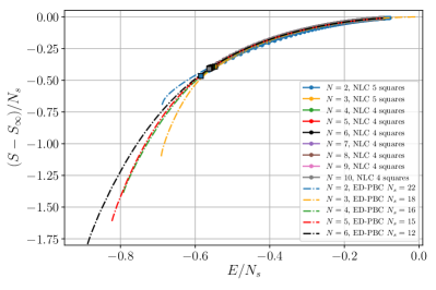
Figure 6: Entropy per site as a function of the energy per site for the SU$(N)$ Heisenberg model on the square lattice. The full lines with the filled circles denote NLC results, while the dot-dashed lines denote complete numerical diagonalizations for periodic finite size clusters. The circles are plotted at the $(s,e)$ coordinate corresponding to $T/J=1/2$ for all $N$.

V Equation of state on the square lattice

In the discussion so far we used only the temperature $T/J$ as a control parameter of the thermal equilibrium. However in the ultracold atom context it is also useful to understand the physics in terms of the entropy $S$ or the entropy per site $s$. In order to address the entropy dependence of the correlations (as e.g. studied in Ref. Messio and Mila (2012) for one dimensional SU$(N)$ chains) we numerically determine the entropy per site $s\equiv S/N_{s}$ as a function of the energy density $e\equiv E/N_{s}$. This function $s(e)$ is known to be a thermodynamic potential, and allows therefore to extract e.g. the temperature via

$$\frac{ds}{de}=\frac{1}{T(e)}\ .$$

We note that for our nearest neighbour spin Hamiltonians (2) the energy per site $e=\frac{z}{2}\ C_{\mathrm{spin}}(n.n.)$ is related to the nearest neighbor spin correlator discussed above via the coordination number $z$ of the lattice.

We calculated the entropy $S(T)$ and the energy $E(T)$ from the finite size partition function obtained by complete numerical diagonalizations of periodic square lattice systems. Furthermore we have implemented a numerical linked cluster expansion based on a real space cluster expansion in terms of squares Rigol et al. (2007), while the complete numerical diagonalizations required for each cluster were performed in the SU$(N)$ Young tableau basis Nataf and Mila (2014).

In Fig. 6 we show the resulting curves $s(e)$ for various $N$ between $2$ and $10$ for the square lattice. We chose the origin of the $y$-axis at the infinite temperature reference value $\ln(N)$. We have indicated the $(s,e)$ coordinates corresponding to $T/J=1/2$ with filled squares in Fig. 6. Curiously we observe that almost all curves lie on top of each other in the regime corresponding to high temperature. The consequence of this observation is that in the high temperature regime of SU$(N)$ Heisenberg models one has to shelve away an $N$-independent amount of entropy per site to cool to the same temperature (here $T/J=1/2$ as an example). Obviously this is not true when cooling to the ground state, as then the full entropy per site of $\ln(N)$ has to be removed.

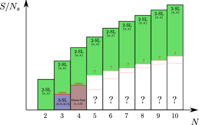
Figure 7: Schematic phase diagram of the SU($N$) Heisenberg model on the square lattice for $N\leq 10$. The maximum achievable entropy per site for a given $N$ is $\log N$ (corresponding to $T\rightarrow\infty$) signalized by the height of the bars.

Our leading order high temperature series expansion result (6) allows us to understand the origin of this phenomenon. In this expansion the nearest neighbour correlations ($m=1$) depend on $N$ as $(1-1/N^{2})$, becoming basically $N$-independent rather quickly. On the one hand this correlator is proportional to the energy $e$, and on the other hand we can determine the entropy reduction away from infinite temperature from an integration of the specific heat per site $c(T)=de/dT$:

$$\Delta s(T)=\ln(N)-s(T)=\int_{T}^{\infty}\frac{c(\tau)}{\tau}d\tau$$

We thus see that the approximate $N$-independence of the nearest-neighbor correlator in the Manhattan regime, and its relevance for the energy, implies that the entropy reduction to reach a certain final temperature is approximately $N$-independent on the type of lattices considered in this work.

This also explains the two apparently conflicting results regarding one-dimensional chains, that the Lifshitz temperatures are almost independent of $N$ according to Ref. Fukushima and Kuramoto (2002), while Ref. Messio and Mila (2012) reports an increasing entropy per site for the Lifshitz points. Here we see that the two point of views coincide when viewed from infinite temperature, but seem to diverge when viewed from zero temperature.

Unfortunately our methods do not allow us to systematically and reliably study the low temperature physics of large $N$ and $N_{s}$ systems, so a large fraction of the $s$-$N$ phase diagram for the square lattice in Fig. 7 has to remain uncharted. However our work has substantiated an extended region in temperature or entropy where the correlations are short-ranged and structured in real-space according to the Manhattan structure. This region is indicated in green in Fig. 7. For $N=2$ this Manhattan region is continuously connected to the low temperature region with an exponentially diverging correlation length for the same structure of correlations. For $N=3$ and $N=4$ we have worked out the approximate location of the Lifshitz or first order transitions to a different low-temperature regime in Sec. IV.2. For larger $N$ we are unable to reliably estimate the lower end of the Manhattan region.

VI Conclusion

In this work we have analyzed the real-space structure of spin correlations in the SU$(N)$ Heisenberg model with spins in the fundamental representation on a broad range of lattices. We find a unifying pattern, the Manhattan structure, where spin correlations are organized in shells of equal Manhattan distance, and alternating in sign from one shell to the next.

For selected case we have investigated how the Manhattan regime breaks down at low temperature through indicators such as the disorder or Lifshitz temperature.

Investigating the dependence of the entropy reduction from the infinite temperature value of $\ln(N)$, we have realized that the Manhattan regime is governed by an approximately $N$-independent equation of state, see Fig. 6. This has interesting consequences, such that the entropy reduction from $\ln(N)$ to reach a certain temperature in the Manhattann regime is approximately $N$ independent, potentially easing the way to reach low temperatures in the SU$(N)$ spin models, akin to the Pomeranchuk cooling effect discussed previously Hazzard et al. (2012); Taie et al. (2012); Cai et al. (2013).

An important open question remains however. While reaching low temperatures in the Manhattan regime seems easy, it is not clear how easy it will be to go to even lower temperatures where more $N$ specific novel physics can be reached. For example in the one-dimensional chains the SU$(N)$ Wess-Zumino-Witten regime predicted at zero temperature is visible only at temperatures which decrease with $N$, as discussed in Ref. Fukushima and Kuramoto (2002). The temperatures we report to reach the ground state physics of the SU$(3)$ and SU$(4)$ square lattices with $T_{L}/J\approx 0.18$ and $T_{L}/J\approx 0.23$ are already quite low.

Acknowledgments

AML thanks S. Fölling for discussions which motivated the present investigation. We acknowledge support by the Austrian Science Fund (project IDs: F-4018 and I-2868). The computational results presented have been achieved in part using the Vienna Scientific Cluster (VSC). This work was supported by the Austrian Ministry of Science BMWF as part of the UniInfrastrukturprogramm of the Focal Point Scientific Computing at the University of Innsbruck. We acknowledge PRACE for granting access to ”Joliot Curie” HPC resources at TGCC/CEA under grant number 2019204846.

Appendix A Observables for SU$(N)$ spin correlations

In this section we discuss the relation between several observables which are useful to quantify spin correlations for SU$(N)$ quantum spin systems with local spins in the $N$-dimensional fundamental ( ${\tiny\yng(1)}$ ) irreducible representation of SU$(N)$. Assuming an arbitrary state $\rho$ of the entire system which is SU$(N)$ invariant (e.g. an SU$(N)$ singlet pure state, or a non-symmetry-broken thermal density matrix), the two site reduced density matrix $\rho_{i,j}=\operatorname{Tr}_{E(i,j)}\left[\rho\right]$, (where $E(i,j)$ denotes all remaining degrees of freedom apart from sites $i$ and $j$) contains all the information regarding correlations between sites $i$ and $j$. The two site reduced density matrix of linear dimension $N^{2}$ has two subspaces: the symmetric subspace (${\tiny\yng(2)}$) of dimension $N(N+1)/2$ and the antisymmetric (${\tiny\yng(1,1)}$) of dimension $N(N-1)/2$. The total weight of the state on the symmetric and the antisymmetric subspaces are denoted $p_{S}$ and $p_{A}$ respectively, with $p_{S}+p_{A}=1$.

Let us now discuss a few observables and their relation to $p_{S}$ and $p_{A}$. We use the notation $\langle\mathcal{O}_{i,j}\rangle=\operatorname{Tr}\left[\mathcal{O}_{i,j}\rho_{i,j}\right]$.

1. The two site permutation operator $P_{ij}$ is particularly simple in this respect. The operator has eigenvalue $+1$ $(-1)$ in the symmetric (antisymmetric) subspace.

   $$C_{P}(i,j)\equiv\langle P_{i,j}\rangle=p_{S}-p_{A}$$ (8)

   At infinite temperature, the two-site reduced density matrix is proportional to the identity: $\rho_{i,j}(T{=}\infty)=\mathbb{1}/{N^{2}}$. This leads to $p_{S}=\frac{N(N+1)}{2N^{2}}$ and $p_{A}=\frac{N(N-1)}{2N^{2}}$. Thus the correlator: $C_{P}(i,j)=1/N$ at $T=\infty.$

2. The contraction of SU$(N)$ spin operators which we use in the Hamiltonian Eq. (2) are related to the permutation operator as outlined in Eq. (3). This leads to the following correlations:

   $$C_{\mathrm{spin}}(i,j) = \langle\sum_{A}S^{A}_{i}S^{A}_{j}\rangle$$

   $$= \tfrac{1}{2}(C_{P}(i,j)-\tfrac{1}{N})$$

   $$= \tfrac{1}{2}(p_{S}-p_{A}-1/N)$$

   This operator reduces to the well-known $\mathbf{S}_{i}\cdot\mathbf{S}_{j}$ operator for $S{=}1/2$ for SU$(2)$, yielding $C_{\mathrm{spin}}(i,j)=-3/4\ (+1/4)$ for an SU$(2)$ singlet (triplet).

   At infinite temperature this correlation vanishes for all $N$: $C_{\mathrm{spin}}(i,j)=0$ at $T=\infty$.

3. In the recent ”Singlet-Triplet-Oscillations” (STO) experiments for SU$(2)$ and SU$(N{>}2)$ systems Greif et al. (2013); Ozawa et al. (2018); Takahashi (2018, 2020) it is possible to estimate the symmetric ($p_{S}$, ”triplet”) and the antisymmetric ($p_{A}$, ”singlet”) fraction of a nearest neighbour density matrix on several lattices (e.g. honeycomb, cubic). We refer to those references for the details of the method.

4. We anticipate that in future quantum gas microscopes it will be possible to record snapshots of the internal spin state configurations of a cloud of atoms, in analogy to what is currently possible for SU$(2)$ fermions in an optical lattice Parsons et al. (2016); Boll et al. (2016); Cheuk et al. (2016); Brown, Peter T. and Mitra, Debayan and Guardado-Sanchez, Elmer and Schauß, Peter and Kondov, Stanimir S. and Khatami, Ehsan and Paiva, Thereza and Trivedi, Nandini and Huse, David A. and Bakr, Waseem S. (2017); Mazurenko et al. (2017). In such experiments it is then possible to measure ”color-color” correlations, i.e. to measure the probability of finding two atoms at sites $i$ and $j$ in the same internal SU$(N)$ spin state $\alpha$.

   We therefore define a diagonal color correlator for SU$(N)$ spin models as

   $$C_{\mathrm{color}}(i,j) = \langle\sum_{\alpha}|\alpha_{i},\alpha_{j}\rangle\langle\alpha_{i},\alpha_{j}|\rangle$$ (10)

   $$= \langle\sum_{\{A\in C\}}2S^{A}_{i}S^{A}_{j}+\tfrac{1}{N}\rangle$$

   where $C$ denotes the set of $N-1$ indices corresponding to the diagonal spin operators $S^{A}_{i}$, $S^{A}_{j}$ on site $i$ and $j$, i.e. the hermitian Cartan generators of the Lie algebra $su(N)$. This observable is a projector and can be seen as the probability to have the same spin color on site $i$ and $j$. For example, in the case of SU$(2)$ and SU$(3)$ the observable reads $C_{\mathrm{color}}(i,j)=2\langle S^{z}_{i}S^{z}_{j}\rangle+1/2$ and $C_{\mathrm{color}}(i,j)=2(\langle S^{3}_{i}S^{3}_{j}\rangle+\langle S^{8}_{i}S^{8}_{j}\rangle)+1/3$, respectively.

   Due to the SU$(N)$ symmetry the expectation value $\langle S^{A}_{i}S^{A}_{j}\rangle$ is the same for every component $A$ and hence $\langle\sum_{A}S^{A}_{i}S^{A}_{j}\rangle=(N^{2}-1)\langle S^{0}_{i}S^{0}_{j}\rangle$. After some algebraic steps one obtains the relation of the diagonal color correlator with the two site permutation operator

   $$C_{\mathrm{color}}(i,j) = \tfrac{1}{N}+\tfrac{N-1}{N^{2}-1}(\langle P_{ij}\rangle-\tfrac{1}{N})$$ (11)

   $$= \tfrac{1}{N}+\tfrac{1}{N+1}(p_{S}-p_{A}-\tfrac{1}{N})$$

   At infinite temperature the $C_{\mathrm{color}}(i,j)$ correlator takes the value $1/N$.

Appendix B Microcanonical Analysis

The material in the main text is derived from the canonical Gibbs ensemble. In this appendix we highlight selected results for spin correlations on square lattice clusters, where large-scale numerical full diagonalizations exploiting the SU$(N)$ symmetry Nataf and Mila (2014) have been carried out. In Fig. 8 we show results for a spatially symmetric 18 sites square cluster for the SU$(3)$ Heisenberg model. This cluster has periodic boundary conditions and is spanned by the simulation cell vectors $\mathbf{T}_{1}=(3,3)$ and $\mathbf{T}_{2}=(-3,3)$. The entire Hilbert space has a dimension of $3^{18}=387\ 420\ 489$. After dividing the Hilbert space into SU$(N)$ irreducible representations, the largest matrix size to be diagonalized features a dimension of almost $800\ 000$. The panels are arranged according to the position of the second site in the correlator with the origin. In each panel we show a two-dimensional histogram compiled from all $3^{18}$ eigenstates of the system, where on the $x$ axis the energy per site $E/N_{s}$ is plotted, while on the $y$ axis the value of the corresponding correlator $C_{\mathrm{spin}}(\Delta x,\Delta y)$. Furthermore we plot the energy-correlator behaviour of the canonical predictions in the temperature range $T=0$ to $T=\infty$, based on the same finite size data (dark green, dashed line). The positive energy per site region corresponds to the ferromagnetic side of the energy spectrum. One can see how the ferromagnetic correlations build up as one approaches the maximum energy per site ($E/N_{s}=2/3$). On the antiferromagnetic side of the energy spectrum the behaviour of the correlators is less regular, but one can recognize that at low energy, the distribution of the correlators starts to concentrate and converge towards the $T=0$, i.e. ground state results, where the canonical and the microcanonical predictions match.

Overall one can see that the expected eigenstate thermalization hypothesis (ETH) Deutsch (1991); Srednicki (1994); Beugeling et al. (2014) behaviour is not fully reached yet for this system size, despite the huge total Hilbert space. We attribute this to the large amount of different quantum number sectors (spatial symmetry sectors combined with SU$(3)$ representations) which contribute to the observables, and which are all included in the plots.

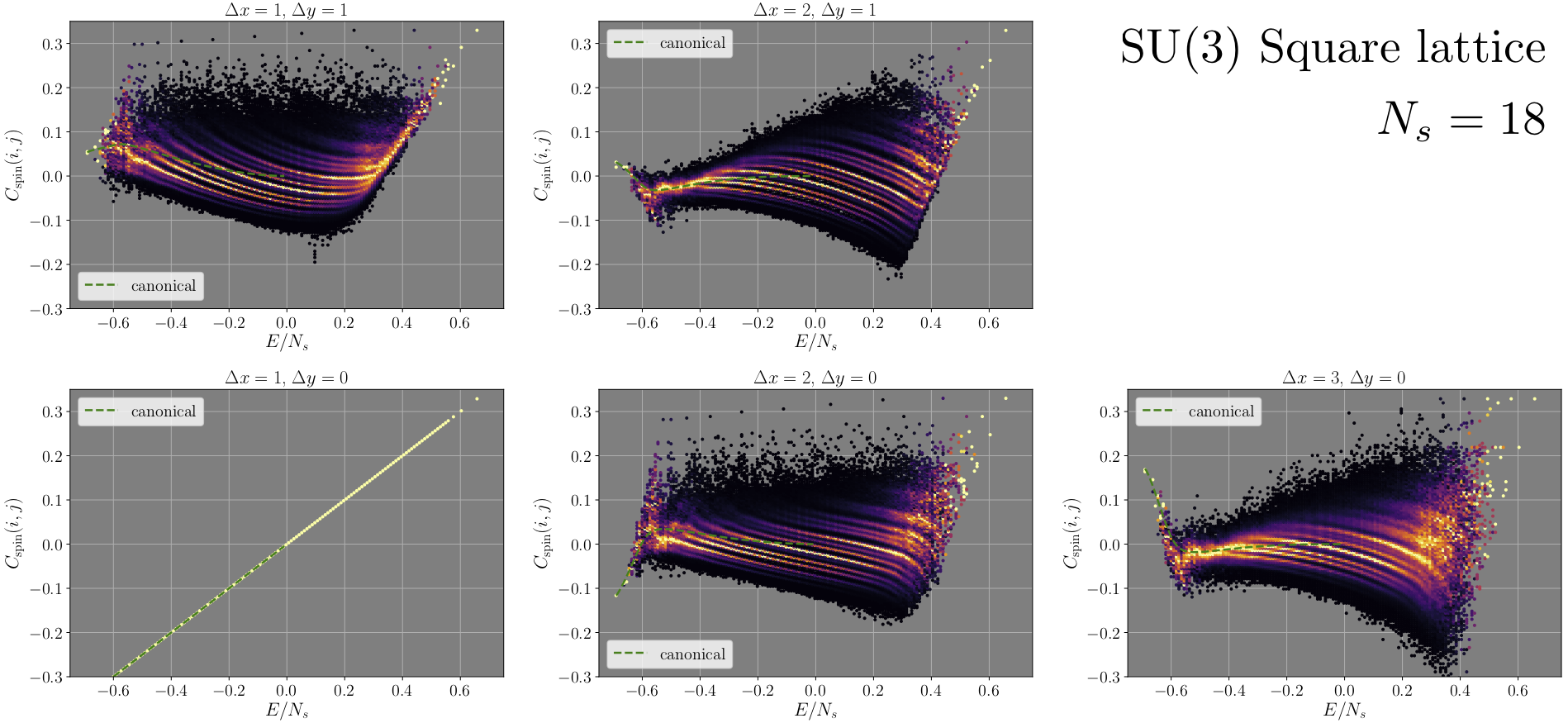
Figure 8: Microcanonical analysis of spin correlations for the SU$(3)$ Heisenberg model on a 18 sites square lattice cluster, For a detailed description see App. B.

Appendix C Continuous structure factor ansatz

In this section we perform an continuous structure factor ansatz and thereby estimate the Lifshitz temperature under the assumption that coming from high temperatures a Lifshitz transition occurs. We focus on the 2D square lattice but for the one-dimensional chain the derivation is perfomed in an analog way. We start by decomposing the static structure factor of the spin-spin correlations on the infinite square lattice into harmonics

$$S(\mathbf{k})={\sum_{j\neq 1}}^{\prime}2\cos[\mathbf{k}(\mathbf{r}_{j}-\mathbf{r}_{0})]\left<\mathbf{S}_{j}\mathbf{S}_{1}\right>+\frac{N^{2}-1}{2N},$$ (12)

where the sum ${\sum}^{\prime}$ runs over the subset corresponding to the indices of one quadrant of the lattice, centered by the reference site $\mathbf{r}_{0}$. We cut the series at distance three and set correlations for larger distances to zero by definition

$$S(\mathbf{k}) = c_{0}+c_{1}[\cos(k_{x})+\cos(k_{y})]$$ (13)

$$+ c_{2}[\cos(2k_{x})+\cos(2k_{y})]$$

$$+ c_{3}[\cos(k_{x}+k_{y})+\cos(k_{x}-k_{y})]$$

$$+ c_{4}[\cos(3k_{x})+\cos(3k_{y})]$$

$$+ c_{5}[\cos(2k_{x}+k_{y})+\cos(2k_{x}-k_{y})$$

$$+ \cos(k_{x}+2k_{y})+\cos(k_{x}-2k_{y})],$$

where $c_{j}=2\,C_{\mathrm{spin}}(0,j)$. Taylor expanding around $(\pi,\pi)$ and keeping maximally quartic terms leads to the following Ginzburg-Landau free energy like expression

$$S((\pi+x,\pi+y))\approx\;a_{0}+a_{1}(x^{2}+y^{2})+a_{2}(x^{4}+y^{4})+a_{3}x^{2}y^{2}$$ (14)

with

$$\begin{split}a_{0}&=c_{0}-2c_{1}+2c_{2}+2c_{3}-2c_{4}-4c_{5}\\ a_{1}&=\frac{c_{1}}{2}-2c_{2}-c_{3}+\frac{9c_{4}}{2}+5c_{5}\\ a_{2}&=-\frac{c_{1}}{24}+\frac{2c_{2}}{3}+\frac{c_{3}}{12}-\frac{27c_{4}}{8}-\frac{17c_{5}}{12}\\ a_{3}&=\frac{c_{3}}{2}-4c_{5}.\end{split}$$ (15)

By maximizing Eq. (14) we find three different regimes: (I) a trivial regime with the maximum at $(\pi,\pi)$, (II) a second regime with four maxima along the diagonals ($(\pi\pm\epsilon,\pi\pm\epsilon)$ with $\epsilon=\sqrt{-a_{1}/(2a_{2}+a_{3})}$) through $(\pi,\pi)$ and (III) a third regime with four maxima along horizontal and vertical lines ($(0,\pi\pm\epsilon)$ and $(\pi\pm\epsilon,0)$ with $\epsilon=\sqrt{-a_{1}/(2a_{2})}$) through $(\pi,\pi)$. Finally, by matching the coefficients ${a_{i}}$ with the ED data for our largest cluster for every temperature we obtain a trajectory in the coefficient space. Starting from the origin ($T\rightarrow\infty$) the trajectory moves into the trivial regime, where the structure factor is peaked at $(\pi,\pi)$, but bends back and breaks through regime (II) at $T_{L}(\infty)/J=0.180(5)$ for SU$(3)$ and through regime (III) at $T_{L}(\infty)/J=0.230(5)$ for SU$(4)$, which are the estimated Lifshitz temperatures.

References

- Honerkamp and Hofstetter (2004) C. Honerkamp and W. Hofstetter, “Ultracold Fermions and the Hubbard Model,” Phys. Rev. Lett. 92, 170403 (2004).
- Cazalilla et al. (2009) M. A. Cazalilla, A. F. Ho, and M. Ueda, “Ultracold gases of ytterbium: ferromagnetism and Mott states in an SU(6) Fermi system,” New Journal of Physics 11, 103033 (2009).
- Gorshkov et al. (2010) A. V. Gorshkov, M. Hermele, V. Gurarie, C. Xu, P. S. Julienne, J. Ye, P. Zoller, E. Demler, M. D. Lukin, and A. M. Rey, “Two-orbital SU(N) magnetism with ultracold alkaline-earth atoms,” Nat Phys 6, 289 (2010).
- Sutherland (1975) B. Sutherland, “Model for a multicomponent quantum system,” Phys. Rev. B 12, 3795 (1975).
- Affleck and Marston (1988) I. Affleck and J. B. Marston, “Large-n limit of the Heisenberg-Hubbard model: Implications for high- superconductors,” Phys. Rev. B 37, 3774 (1988).
- Read and Sachdev (1989) N. Read and S. Sachdev, “Valence-bond and spin-Peierls ground states of low-dimensional quantum antiferromagnets,” Phys. Rev. Lett. 62, 1694 (1989).
- Marston and Affleck (1989) J. B. Marston and I. Affleck, “Large- limit of the Hubbard-Heisenberg model,” Phys. Rev. B 39, 11538 (1989).
- Daley (2011) A. J. Daley, “Quantum computing and quantum simulation with group-II atoms,” Quantum Information Processing 10, 865 (2011).
- Cazalilla and Rey (2014) M. A. Cazalilla and A. M. Rey, “Ultracold Fermi gases with emergent SU(N) symmetry,” Reports on Progress in Physics 77, 124401 (2014).
- DeSalvo et al. (2010) B. J. DeSalvo, M. Yan, P. G. Mickelson, Y. N. Martinez de Escobar, and T. C. Killian, “Degenerate Fermi Gas of ,” Phys. Rev. Lett. 105, 030402 (2010).
- Tey et al. (2010) M. K. Tey, S. Stellmer, R. Grimm, and F. Schreck, “Double-degenerate Bose-Fermi mixture of strontium,” Phys. Rev. A 82, 011608 (2010).
- Stellmer et al. (2011) S. Stellmer, R. Grimm, and F. Schreck, “Detection and manipulation of nuclear spin states in fermionic strontium,” Phys. Rev. A 84, 043611 (2011).
- (13) S. Stellmer, F. Schreck, and T. C. Killian, “Degenerate Quantum Gases of Strontium,” in Annual Review of Cold Atoms and Molecules, Chap. 1, pp. 1–80.
- Zhang et al. (2014) X. Zhang, M. Bishof, S. L. Bromley, C. V. Kraus, M. S. Safronova, P. Zoller, A. M. Rey, and J. Ye, “Spectroscopic observation of SU(N)-symmetric interactions in Sr orbital magnetism,” Science 345, 1467 (2014).
- Qi et al. (2019) W. Qi, M.-C. Liang, H. Zhang, Y.-D. Wei, W.-W. Wang, X.-J. Wang, and X. Zhang, “Experimental Realization of Degenerate Fermi Gases of 87Sr Atoms with 10 or Two Spin Components,” Chinese Physics Letters 36, 093701 (2019).
- Sonderhouse et al. (2020) L. Sonderhouse, C. Sanner, R. B. Hutson, A. Goban, T. Bilitewski, L. Yan, W. R. Milner, A. M. Rey, and J. Ye, “Thermodynamics of a deeply degenerate SU()-symmetric Fermi gas,” arXiv e-prints , arXiv:2003.02408 (2020), arXiv:2003.02408 [cond-mat.quant-gas] .
- Bataille et al. (2020) P. Bataille, A. Litvinov, I. Manai, J. Huckans, F. Wiotte, A. Kaladjian, O. Gorceix, E. Maréchal, B. Laburthe-Tolra, and M. Robert-de-Saint-Vincent, “Adiabatic spin-dependent momentum transfer in an SU(N) degenerate Fermi gas,” arXiv e-prints , arXiv:2003.13444 (2020), arXiv:2003.13444 [cond-mat.quant-gas] .
- Fukuhara et al. (2007) T. Fukuhara, Y. Takasu, M. Kumakura, and Y. Takahashi, “Degenerate Fermi Gases of Ytterbium,” Phys. Rev. Lett. 98, 030401 (2007).
- Taie et al. (2010) S. Taie, Y. Takasu, S. Sugawa, R. Yamazaki, T. Tsujimoto, R. Murakami, and Y. Takahashi, “Realization of a System of Fermions in a Cold Atomic Gas,” Phys. Rev. Lett. 105, 190401 (2010).
- Sugawa et al. (2011) S. Sugawa, K. Inaba, S. Taie, R. Yamazaki, M. Yamashita, and Y. Takahashi, “Interaction and filling-induced quantum phases of dual Mott insulators of bosons and fermions,” Nat Phys 7, 642 (2011).
- Pagano et al. (2014) G. Pagano, M. Mancini, G. Cappellini, P. Lombardi, F. Schäfer, H. Hu, X.-J. Liu, J. Catani, C. Sias, M. Inguscio, and L. Fallani, “A one-dimensional liquid of fermions with tunable spin,” Nature Physics 10, 198 (2014).
- He et al. (2020) C. He, Z. Ren, B. Song, E. Zhao, J. Lee, Y.-C. Zhang, S. Zhang, and G.-B. Jo, “Collective excitations in two-dimensional su() fermi gases with tunable spin,” Phys. Rev. Research 2, 012028 (2020).
- Taie et al. (2012) S. Taie, R. Yamazaki, S. Sugawa, and Y. Takahashi, “An SU(6) Mott insulator of an atomic Fermi gas realized by large-spin Pomeranchuk cooling,” Nat. Phys 8, 825 (2012).
- Hofrichter et al. (2016) C. Hofrichter, L. Riegger, F. Scazza, M. Höfer, D. R. Fernandes, I. Bloch, and S. Fölling, “Direct Probing of the Mott Crossover in the Fermi-Hubbard Model,” Phys. Rev. X 6, 021030 (2016).
- Jördens et al. (2008) R. Jördens, N. Strohmaier, K. Günter, H. Moritz, and T. Esslinger, “A Mott insulator of fermionic atoms in an optical lattice,” Nature 455, 204 (2008).
- Schneider et al. (2008) U. Schneider, L. Hackermüller, S. Will, T. Best, I. Bloch, T. A. Costi, R. W. Helmes, D. Rasch, and A. Rosch, “Metallic and Insulating Phases of Repulsively Interacting Fermions in a 3D Optical Lattice,” Science 322, 1520 (2008).
- Greif et al. (2013) D. Greif, T. Uehlinger, G. Jotzu, L. Tarruell, and T. Esslinger, “Short-Range Quantum Magnetism of Ultracold Fermions in an Optical Lattice,” Science 340, 1307 (2013).
- Parsons et al. (2016) M. F. Parsons, A. Mazurenko, C. S. Chiu, G. Ji, D. Greif, and M. Greiner, “Site-resolved measurement of the spin-correlation function in the Fermi-Hubbard model,” Science 353, 1253 (2016).
- Boll et al. (2016) M. Boll, T. A. Hilker, G. Salomon, A. Omran, J. Nespolo, L. Pollet, I. Bloch, and C. Gross, “Spin- and density-resolved microscopy of antiferromagnetic correlations in Fermi-Hubbard chains,” Science 353, 1257 (2016).
- Cheuk et al. (2016) L. W. Cheuk, M. A. Nichols, K. R. Lawrence, M. Okan, H. Zhang, E. Khatami, N. Trivedi, T. Paiva, M. Rigol, and M. W. Zwierlein, “Observation of spatial charge and spin correlations in the 2D Fermi-Hubbard model,” Science 353, 1260 (2016).
- Brown, Peter T. and Mitra, Debayan and Guardado-Sanchez, Elmer and Schauß, Peter and Kondov, Stanimir S. and Khatami, Ehsan and Paiva, Thereza and Trivedi, Nandini and Huse, David A. and Bakr, Waseem S. (2017) Brown, Peter T. and Mitra, Debayan and Guardado-Sanchez, Elmer and Schauß, Peter and Kondov, Stanimir S. and Khatami, Ehsan and Paiva, Thereza and Trivedi, Nandini and Huse, David A. and Bakr, Waseem S., “Spin-imbalance in a 2D Fermi-Hubbard system,” Science 357, 1385 (2017).
- Mazurenko et al. (2017) A. Mazurenko, C. S. Chiu, G. Ji, M. F. Parsons, M. Kanász-Nagy, R. Schmidt, F. Grusdt, E. Demler, D. Greif, and M. Greiner, “A cold-atom Fermi-Hubbard antiferromagnet,” Nature 545, 462 (2017).
- Hart et al. (2015) R. A. Hart, P. M. Duarte, T.-L. Yang, X. Liu, T. Paiva, E. Khatami, R. T. Scalettar, N. Trivedi, D. A. Huse, and R. G. Hulet, “Observation of antiferromagnetic correlations in the Hubbard model with ultracold atoms,” Nature 519, 211 (2015).
- Ozawa et al. (2018) H. Ozawa, S. Taie, Y. Takasu, and Y. Takahashi, “Antiferromagnetic Spin Correlation of Fermi Gas in an Optical Superlattice,” Phys. Rev. Lett. 121, 225303 (2018).
- Takahashi (2018) Y. Takahashi, “Quantum Simulation with Ytterbium Fermi Gases,” (2018).
- Takahashi (2020) Y. Takahashi, “Quantum magnetism of SU(6) fermions in an optical lattice,” (2020).
- Miranda et al. (2015) M. Miranda, R. Inoue, Y. Okuyama, A. Nakamoto, and M. Kozuma, “Site-resolved imaging of ytterbium atoms in a two-dimensional optical lattice,” Phys. Rev. A 91, 063414 (2015).
- Miranda et al. (2017) M. Miranda, R. Inoue, N. Tambo, and M. Kozuma, “Site-resolved imaging of a bosonic Mott insulator using ytterbium atoms,” Phys. Rev. A 96, 043626 (2017).
- Knottnerus et al. (2020) I. H. A. Knottnerus, S. Pyatchenkov, O. Onishchenko, A. Urech, F. Schreck, and G. A. Siviloglou, “Microscope objective for imaging atomic strontium with 0.63 micrometer resolution,” Opt. Express 28, 11106 (2020).
- Okuno et al. (2020) D. Okuno, Y. Amano, K. Enomoto, N. Takei, and Y. Takahashi, “Schemes for nondestructive quantum gas microscopy of single atoms in an optical lattice,” New Journal of Physics 22, 013041 (2020).
- Frischmuth et al. (1999) B. Frischmuth, F. Mila, and M. Troyer, “Thermodynamics of the One-Dimensional SU(4) Symmetric Spin-Orbital Model,” Phys. Rev. Lett. 82, 835 (1999).
- Manmana et al. (2011) S. R. Manmana, K. R. A. Hazzard, G. Chen, A. E. Feiguin, and A. M. Rey, “SU magnetism in chains of ultracold alkaline-earth-metal atoms: Mott transitions and quantum correlations,” Phys. Rev. A 84, 043601 (2011).
- Messio and Mila (2012) L. Messio and F. Mila, “Entropy Dependence of Correlations in One-Dimensional Antiferromagnets,” Phys. Rev. Lett. 109, 205306 (2012).
- Bonnes et al. (2012) L. Bonnes, K. R. A. Hazzard, S. R. Manmana, A. M. Rey, and S. Wessel, “Adiabatic Loading of One-Dimensional Alkaline-Earth-Atom Fermions in Optical Lattices,” Phys. Rev. Lett. 109, 205305 (2012).
- Yip et al. (2014) S.-K. Yip, B.-L. Huang, and J.-S. Kao, “Theory of Fermi liquids,” Phys. Rev. A 89, 043610 (2014).
- Decamp et al. (2016) J. Decamp, J. Jünemann, M. Albert, M. Rizzi, A. Minguzzi, and P. Vignolo, “High-momentum tails as magnetic-structure probes for strongly correlated fermionic mixtures in one-dimensional traps,” Phys. Rev. A 94, 053614 (2016).
- Huang et al. (2019) C.-H. Huang, Y. Takasu, Y. Takahashi, and M. A. Cazalilla, “Suppression and Control of Pre-thermalization in Multi-component Fermi Gases Following a Quantum Quench,” arXiv e-prints , arXiv:1910.09750 (2019), arXiv:1910.09750 [cond-mat.quant-gas] .
- Nonne et al. (2013) H. Nonne, M. Moliner, S. Capponi, P. Lecheminant, and K. Totsuka, “Symmetry-protected topological phases of alkaline-earth cold fermionic atoms in one dimension,” EPL (Europhysics Letters) 102, 37008 (2013).
- Rachel et al. (2009) S. Rachel, R. Thomale, M. Führinger, P. Schmitteckert, and M. Greiter, “Spinon confinement and the Haldane gap in spin chains,” Phys. Rev. B 80, 180420 (2009).
- Dufour et al. (2015) J. Dufour, P. Nataf, and F. Mila, “Variational Monte Carlo investigation of Heisenberg chains,” Phys. Rev. B 91, 174427 (2015).
- Capponi et al. (2016) S. Capponi, P. Lecheminant, and K. Totsuka, “Phases of one-dimensional SU(N) cold atomic Fermi gases-From molecular Luttinger liquids to topological phases,” Annals of Physics 367, 50 (2016).
- Tanimoto and Totsuka (2015) K. Tanimoto and K. Totsuka, “Symmetry-protected topological order in SU(N) Heisenberg magnets –quantum entanglement and non-local order parameters,” (2015), arXiv:1508.07601 [cond-mat.str-el] .
- Suzuki et al. (2015) T. Suzuki, K. Harada, H. Matsuo, S. Todo, and N. Kawashima, “Thermal phase transition of generalized Heisenberg models for spins on square and honeycomb lattices,” Phys. Rev. B 91, 094414 (2015).
- Okubo et al. (2015) T. Okubo, K. Harada, J. Lou, and N. Kawashima, “ Heisenberg model with multicolumn representations,” Phys. Rev. B 92, 134404 (2015).
- Motoyama and Todo (2018) Y. Motoyama and S. Todo, “ Berry phase and symmetry-protected topological phases of the SU() antiferromagnetic Heisenberg chain,” Phys. Rev. B 98, 195127 (2018).
- Gauthé et al. (2020) O. Gauthé, S. Capponi, M. Mambrini, and D. Poilblanc, “Quantum spin liquid phases in the bilinear-biquadratic two-SU(4)-fermion Hamiltonian on the square lattice,” (2020), arXiv:2002.05572 [cond-mat.str-el] .
- Sotnikov and Hofstetter (2014) A. Sotnikov and W. Hofstetter, “Magnetic ordering of three-component ultracold fermionic mixtures in optical lattices,” Phys. Rev. A 89, 063601 (2014).
- Sotnikov (2015) A. Sotnikov, “Critical entropies and magnetic-phase-diagram analysis of ultracold three-component fermionic mixtures in optical lattices,” Phys. Rev. A 92, 023633 (2015).
- Yanatori and Koga (2016) H. Yanatori and A. Koga, “Finite-temperature phase transitions in the Hubbard model,” Phys. Rev. B 94, 041110 (2016).
- Golubeva et al. (2017) A. Golubeva, A. Sotnikov, A. Cichy, J. Kuneš, and W. Hofstetter, “Breaking of SU(4) symmetry and interplay between strongly correlated phases in the Hubbard model,” Phys. Rev. B 95, 125108 (2017).
- Kanász-Nagy et al. (2017) M. Kanász-Nagy, I. Lovas, F. Grusdt, D. Greif, M. Greiner, and E. A. Demler, “Quantum correlations at infinite temperature: The dynamical Nagaoka effect,” Phys. Rev. B 96, 014303 (2017).
- Assaad (2005) F. F. Assaad, “Phase diagram of the half-filled two-dimensional Hubbard-Heisenberg model: A quantum Monte Carlo study,” Phys. Rev. B 71, 075103 (2005).
- Hazzard et al. (2012) K. R. A. Hazzard, V. Gurarie, M. Hermele, and A. M. Rey, “High-temperature properties of fermionic alkaline-earth-metal atoms in optical lattices,” Phys. Rev. A 85, 041604 (2012).
- Cai et al. (2013) Z. Cai, H.-h. Hung, L. Wang, D. Zheng, and C. Wu, “Pomeranchuk Cooling of Ultracold Fermions in Optical Lattices,” Phys. Rev. Lett. 110, 220401 (2013).
- Zhou et al. (2014) Z. Zhou, Z. Cai, C. Wu, and Y. Wang, “Quantum Monte Carlo simulations of thermodynamic properties of ultracold fermions in optical lattices,” Phys. Rev. B 90, 235139 (2014).
- Wang et al. (2014) D. Wang, Y. Li, Z. Cai, Z. Zhou, Y. Wang, and C. Wu, “Competing Orders in the 2D Half-Filled Hubbard Model through the Pinning-Field Quantum Monte Carlo Simulations,” Phys. Rev. Lett. 112, 156403 (2014).
- Lee et al. (2018) S.-S. B. Lee, J. von Delft, and A. Weichselbaum, “Filling-driven Mott transition in Hubbard models,” Phys. Rev. B 97, 165143 (2018).
- Tamura and Katsura (2019) K. Tamura and H. Katsura, “Ferromagnetism in the Hubbard model with a nearly flat band,” Phys. Rev. B 100, 214423 (2019).
- Chung and Corboz (2019) S. S. Chung and P. Corboz, “SU(3) fermions on the honeycomb lattice at filling,” Phys. Rev. B 100, 035134 (2019).
- Choudhury et al. (2020) S. Choudhury, K. R. Islam, Y. Hou, J. A. Aman, T. C. Killian, and K. R. A. Hazzard, “Collective modes of ultracold fermionic alkaline-earth gases with SU(N) symmetry,” (2020), arXiv:2001.09503 [cond-mat.quant-gas] .
- Fukushima and Kuramoto (2002) N. Fukushima and Y. Kuramoto, “High Temperature Expansion for the SU(n) Heisenberg Model in One Dimension,” Journal of the Physical Society of Japan 71, 1238 (2002).
- Fukushima (2003) N. Fukushima, “A New Method of the High Temperature Series Expansion,” Journal of Statistical Physics 111, 1049 (2003).
- Fukushima (2005) N. Fukushima, “Vanishing Neel Ordering of SU(n) Heisenberg Model in Three Dimensions,” arXiv e-prints , cond-mat/0502484 (2005), arXiv:cond-mat/0502484 [cond-mat.str-el] .
- Nataf and Mila (2014) P. Nataf and F. Mila, “Exact Diagonalization of Heisenberg Models,” Phys. Rev. Lett. 113, 127204 (2014).
- Nataf et al. (2016a) P. Nataf, M. Lajkó, P. Corboz, A. M. Läuchli, K. Penc, and F. Mila, “Plaquette order in the SU(6) Heisenberg model on the honeycomb lattice,” Phys. Rev. B 93, 201113 (2016a).
- van den Bossche et al. (2000) M. van den Bossche, F.-C. Zhang, and F. Mila, “Plaquette ground state in the two-dimensional SU(4) spin-orbital model,” The European Physical Journal B - Condensed Matter and Complex Systems 17, 367 (2000).
- van den Bossche et al. (2001) M. van den Bossche, P. Azaria, P. Lecheminant, and F. Mila, “Spontaneous Plaquette Formation in the SU(4) Spin-Orbital Ladder,” Phys. Rev. Lett. 86, 4124 (2001).
- Penc et al. (2003) K. Penc, M. Mambrini, P. Fazekas, and F. Mila, “Quantum phase transition in the SU(4) spin-orbital model on the triangular lattice,” Phys. Rev. B 68, 012408 (2003).
- Läuchli et al. (2006) A. Läuchli, F. Mila, and K. Penc, “Quadrupolar Phases of the Bilinear-Biquadratic Heisenberg Model on the Triangular Lattice,” Phys. Rev. Lett. 97, 087205 (2006).
- Hermele et al. (2009) M. Hermele, V. Gurarie, and A. M. Rey, “Mott Insulators of Ultracold Fermionic Alkaline Earth Atoms: Underconstrained Magnetism and Chiral Spin Liquid,” Phys. Rev. Lett. 103, 135301 (2009).
- Tóth et al. (2010) T. A. Tóth, A. M. Läuchli, F. Mila, and K. Penc, “Three-Sublattice Ordering of the SU(3) Heisenberg Model of Three-Flavor Fermions on the Square and Cubic Lattices,” Phys. Rev. Lett. 105, 265301 (2010).
- Tóth et al. (2012) T. A. Tóth, A. M. Läuchli, F. Mila, and K. Penc, “Erratum: Three-Sublattice Ordering of the SU(3) Heisenberg Model of Three-Flavor Fermions on the Square and Cubic Lattices [Phys. Rev. Lett. 105, 265301 (2010)],” Phys. Rev. Lett. 108, 029902 (2012).
- Corboz et al. (2011) P. Corboz, A. M. Läuchli, K. Penc, M. Troyer, and F. Mila, “Simultaneous Dimerization and SU(4) Symmetry Breaking of 4-Color Fermions on the Square Lattice,” Phys. Rev. Lett. 107, 215301 (2011).
- Hermele and Gurarie (2011) M. Hermele and V. Gurarie, “Topological liquids and valence cluster states in two-dimensional SU magnets,” Phys. Rev. B 84, 174441 (2011).
- Corboz et al. (2012a) P. Corboz, K. Penc, F. Mila, and A. M. Läuchli, “Simplex solids in SU() Heisenberg models on the kagome and checkerboard lattices,” Phys. Rev. B 86, 041106 (2012a).
- Corboz et al. (2012b) P. Corboz, M. Lajkó, A. M. Läuchli, K. Penc, and F. Mila, “Spin-Orbital Quantum Liquid on the Honeycomb Lattice,” Phys. Rev. X 2, 041013 (2012b).
- Bauer et al. (2012) B. Bauer, P. Corboz, A. M. Läuchli, L. Messio, K. Penc, M. Troyer, and F. Mila, “Three-sublattice order in the SU(3) Heisenberg model on the square and triangular lattice,” Phys. Rev. B 85, 125116 (2012).
- Corboz et al. (2013) P. Corboz, M. Lajkó, K. Penc, F. Mila, and A. M. Läuchli, “Competing states in the SU(3) Heisenberg model on the honeycomb lattice: Plaquette valence-bond crystal versus dimerized color-ordered state,” Phys. Rev. B 87, 195113 (2013).
- Song and Hermele (2013) H. Song and M. Hermele, “Mott insulators of ultracold fermionic alkaline earth atoms in three dimensions,” Phys. Rev. B 87, 144423 (2013).
- Nataf et al. (2016b) P. Nataf, M. Lajkó, A. Wietek, K. Penc, F. Mila, and A. M. Läuchli, “Chiral Spin Liquids in Triangular-Lattice Fermionic Mott Insulators with Artificial Gauge Fields,” Phys. Rev. Lett. 117, 167202 (2016b).
- Weichselbaum et al. (2018) A. Weichselbaum, S. Capponi, P. Lecheminant, A. M. Tsvelik, and A. M. Läuchli, “Unified phase diagram of antiferromagnetic SU() spin ladders,” Phys. Rev. B 98, 085104 (2018).
- Keselman et al. (2019) A. Keselman, B. Bauer, C. Xu, and C.-M. Jian, “Emergent Fermi surface in a triangular-lattice SU(4) quantum antiferromagnet,” arXiv e-prints , arXiv:1912.01025 (2019), arXiv:1912.01025 [cond-mat.str-el] .
- Boos et al. (2020) C. Boos, C. J. Ganahl, M. Lajkó, P. Nataf, A. M. Läuchli, K. Penc, K. P. Schmidt, and F. Mila, “Time-reversal symmetry breaking Abelian chiral spin liquid in Mott phases of three-component fermions on the triangular lattice,” Phys. Rev. Research 2, 023098 (2020).
- Note (1) The inclusion of the clock state leads to a multi-orbital SU Hubbard model, which is interesting in itself Scazza et al. (2014); Cappellini et al. (2014); Höfer et al. (2015); Riegger et al. (2018), but not the topic of the present work.
- Note (2) This is the formula valid for the fundamental representation. At higher order in new terms in the spin model can be generated (see e.g. Boos et al. (2020)), but we stick to the Heisenberg term here.
- Oitmaa et al. (2006) J. Oitmaa, C. Hamer, and W. Zheng, Series expansion methods for strongly interacting lattice models (Cambridge University Press, 2006).
- Rigol et al. (2007) M. Rigol, T. Bryant, and R. R. P. Singh, “Numerical linked-cluster algorithms. I. Spin systems on square, triangular, and kagomé lattices,” Phys. Rev. E 75, 061118 (2007).
- Note (3) The autocorrelation is independent of temperature: .
- Lienhard et al. (2018) V. Lienhard, S. de Léséleuc, D. Barredo, T. Lahaye, A. Browaeys, M. Schuler, L.-P. Henry, and A. M. Läuchli, “Observing the Space- and Time-Dependent Growth of Correlations in Dynamically Tuned Synthetic Ising Models with Antiferromagnetic Interactions,” Phys. Rev. X 8, 021070 (2018).
- Note (4) Where applicable we have divided the numerical results by , in order to simplify the presentation. The ED cluster have periodic boundary conditions and range in size from 12 to 18, depending on the value of .
- Stephenson (1969) J. Stephenson, “Close-packed anisotropic antiferromagnetic Ising lattices. I,” Canadian Journal of Physics 47, 2621 (1969).
- Stephenson (1970) J. Stephenson, “Ising-Model Spin Correlations on the Triangular Lattice. IV. Anisotropic Ferromagnetic and Antiferromagnetic Lattices,” Journal of Mathematical Physics 11, 420 (1970).
- Schollwöck et al. (1996) U. Schollwöck, T. Jolicœur, and T. Garel, “Onset of incommensurability at the valence-bond-solid point in the S=1 quantum spin chain,” Phys. Rev. B 53, 3304 (1996).
- Note (5) We also observe some small modulation in with a period three.
- Mermin and Wagner (1966) N. D. Mermin and H. Wagner, “Absence of Ferromagnetism or Antiferromagnetism in One- or Two-Dimensional Isotropic Heisenberg Models,” Phys. Rev. Lett. 17, 1133 (1966).
- Hohenberg (1967) P. C. Hohenberg, “Existence of Long-Range Order in One and Two Dimensions,” Phys. Rev. 158, 383 (1967).
- Chandra et al. (1990) P. Chandra, P. Coleman, and A. I. Larkin, “Ising transition in frustrated Heisenberg models,” Phys. Rev. Lett. 64, 88 (1990).
- Weber et al. (2003) C. Weber, L. Capriotti, G. Misguich, F. Becca, M. Elhajal, and F. Mila, “Ising Transition Driven by Frustration in a 2D Classical Model with Continuous Symmetry,” Phys. Rev. Lett. 91, 177202 (2003).
- Fang et al. (2008) C. Fang, H. Yao, W.-F. Tsai, J. Hu, and S. A. Kivelson, “Theory of electron nematic order in LaFeAsO,” Phys. Rev. B 77, 224509 (2008).
- Xu et al. (2008) C. Xu, M. Müller, and S. Sachdev, “Ising and spin orders in the iron-based superconductors,” Phys. Rev. B 78, 020501 (2008).
- (111) “Scalapack - scalable linear algebra package,” .
- Tsunetsugu and Arikawa (2006) H. Tsunetsugu and M. Arikawa, “Spin Nematic Phase in S=1 Triangular Antiferromagnets,” Journal of the Physical Society of Japan 75, 083701 (2006).
- Deutsch (1991) J. M. Deutsch, “Quantum statistical mechanics in a closed system,” Phys. Rev. A 43, 2046 (1991).
- Srednicki (1994) M. Srednicki, “Chaos and quantum thermalization,” Phys. Rev. E 50, 888 (1994).
- Beugeling et al. (2014) W. Beugeling, R. Moessner, and M. Haque, “Finite-size scaling of eigenstate thermalization,” Phys. Rev. E 89, 042112 (2014).
- Scazza et al. (2014) F. Scazza, C. Hofrichter, M. Höfer, P. C. De Groot, I. Bloch, and S. Fölling, “Observation of two-orbital spin-exchange interactions with ultracold SU(N)-symmetric fermions,” Nature Physics 10, 779 (2014).
- Cappellini et al. (2014) G. Cappellini, M. Mancini, G. Pagano, P. Lombardi, L. Livi, M. Siciliani de Cumis, P. Cancio, M. Pizzocaro, D. Calonico, F. Levi, C. Sias, J. Catani, M. Inguscio, and L. Fallani, “Direct Observation of Coherent Interorbital Spin-Exchange Dynamics,” Phys. Rev. Lett. 113, 120402 (2014).
- Höfer et al. (2015) M. Höfer, L. Riegger, F. Scazza, C. Hofrichter, D. R. Fernandes, M. M. Parish, J. Levinsen, I. Bloch, and S. Fölling, “Observation of an Orbital Interaction-Induced Feshbach Resonance in ,” Phys. Rev. Lett. 115, 265302 (2015).
- Riegger et al. (2018) L. Riegger, N. Darkwah Oppong, M. Höfer, D. R. Fernandes, I. Bloch, and S. Fölling, “Localized Magnetic Moments with Tunable Spin Exchange in a Gas of Ultracold Fermions,” Phys. Rev. Lett. 120, 143601 (2018).