Natural Gradient for Combined Loss Using Wavelets

Abstract.

Natural gradients have been widely used in optimization of loss functionals over probability space, with important examples such as Fisher-Rao gradient descent for Kullback-Leibler divergence, Wasserstein gradient descent for transport-related functionals, and Mahalanobis gradient descent for quadratic loss functionals. This note considers the situation in which the loss is a convex linear combination of these examples. We propose a new natural gradient algorithm by utilizing compactly supported wavelets to diagonalize approximately the Hessian of the combined loss. Numerical results are included to demonstrate the efficiency of the proposed algorithm.

1. Introduction

Many problems in partial differential equations and machine learning can be formulated as optimization problems over probability densities. For a domain $\Omega$, let $E(p)$ be a loss or energy functional defined for the probability densities $p$ over $\Omega$. The goal is to find $p^{*}$ that minimizes $E(p)$. A common approach, especially for $E(p)$ with a unique minimum, is to follow the gradient descent (GD) dynamics. However, depending the metric used in the gradient calculation, different gradient descent algorithms exhibit drastically different convergence behavior. The term natural gradient refers to the practice of choosing an appropriate metric depending on the loss functional $E(p)$ as well as the probability space. Below are several well-known examples of natural gradient.

• Wasserstein GD that scales the Euclidean gradient $\frac{\delta E}{\delta p}(p)$ with the metric $-\nabla\cdot(p\nabla)$. Wasserstein GD is typically effective for a loss $E(p)$ that behaves like the square of the 2nd Wasserstein distance.

• Fisher-Rao GD that scales the Euclidean gradient $\frac{\delta E}{\delta p}(p)$ with the diagonal tensor $\mathrm{diag}(p)$. Fisher-Rao GD is quite effective for a loss $E(p)$ such as the Kullback-Leibler divergence $\int p(x)\ln\frac{p(x)}{\mu(x)}\mathrm{d}x$.

• Mahalanobis GD that scales the Euclidean gradient $\frac{\delta E}{\delta p}(p)$ with a positive definite metric $B$. Mahalanobis GD is efficient for a quadratic loss of the form $\frac{1}{2}(p-\mu,A(p-\mu))$ with $B\approx A^{-1}$. In this note, we consider the case that $A$ is a positive semidefinite pseudo-differential operator, for example $A=-\Delta$.

A general principle from these examples is that, for a natural gradient to be effective, the metric used at the density $p$ should be an approximate inverse of the Hessian of the loss $E(p)$ at $p$. In each of these three examples, an approximate inverse of the Hessian can be derived quite explicitly.

1.1. Problem statement.

In several problems from kinetic theory and statistical machine learning, one is faced with a loss or energy functional $E(p)$ that is a linear combination of these three forms mentioned above, i.e.,

$$E(p)=\alpha_{1}E_{1}(p)+\alpha_{2}E_{2}(p)+\alpha_{3}E_{3}(p),$$

where $\alpha_{1},\alpha_{2},\alpha_{3}\geq 0$ and $E_{1}$, $E_{2}$, and $E_{3}$ are of the Wasserstein, Fisher-Rao, and Mahalanobis types, respectively, i.e.,

$$\frac{\delta^{2}E_{1}}{\delta p^{2}}(p)\approx(-\nabla\cdot(p\nabla))^{+},\quad\frac{\delta^{2}E_{2}}{\delta p^{2}}(p)\approx\mathrm{diag}\left(\frac{1}{p}\right),\quad\frac{\delta^{2}E_{3}}{\delta p^{2}}(p)\approx A$$

where $(\cdot)^{+}$ stands for pseudo-inverse. As a result, the Hessian of $E(p)$ has the following approximation

$$\frac{\delta^{2}E}{\delta p^{2}}(p)=\alpha_{1}\frac{\delta^{2}E_{1}}{\delta p^{2}}(p)+\alpha_{2}\frac{\delta^{2}E_{2}}{\delta p^{2}}(p)+\alpha_{3}\frac{\delta^{2}E_{3}}{\delta p^{2}}(p).$$

None of three natural gradients listed above is effective for this combined loss functional, since the inverse of $\frac{\delta^{2}E}{\delta p^{2}}(p)$ looks quite different from $-\nabla\cdot(p\nabla)$, $\mathrm{diag}(p)$, or $A^{-1}$.

An immediate question is design an efficient natural gradient (or even an approximate one) for the combined loss $E(p)$. Due to the efficiency considerations, we prefer this natural gradient to have the following features.

• It utilizes the Hessian information of $E_{1}(p)$, $E_{2}(p)$, and $E_{3}(p)$ in the design of the natural gradient.

• It avoids forming and/or inverting the Hessian $\frac{\delta^{2}E}{\delta p^{2}}(p)$ in order to avoid super-linear costs.

• The computational cost of computing the natural gradient from $\frac{\delta E}{\delta p}(p)$ should be of order $O(n\log^{c}n)$, where $n$ is the number of degrees of freedom used for discretizing $p$.

The main idea of our approach is to diagonalize $\frac{\delta^{2}E}{\delta p^{2}}(p)$ approximately by finding a common basis that diagonalizes each of the three terms $\frac{\delta^{2}E_{1}}{\delta p^{2}}(p)$, $\frac{\delta^{2}E_{2}}{\delta p^{2}}(p)$, and $\frac{\delta^{2}E_{3}}{\delta p^{2}}(p)$ approximately at the same time. Among various choices, compactly supported wavelets emerge as a natural candidate because they approximately diagonalize (1) differential operators, (2) diagonal scaling by functions with sufficient regularity, and also (3) pseudo-differential operators.

1.2. Related work.

Fisher-Rao metric is essential to many branches of probability and statistics, as it is invariant under diffeomorphisms. The study of Fishe-Rao and related metrics has evolved to become the field of information geometry and we refer to [amari2016information, ay2017information] for detail discussions. Explicit time-discretization of the Fisher-Rao GD gives rise the mirror descent algorithms [beck2003mirror, bubeck2015convex, nemirovsky1983problem], which plays an essential role in online learning and optimization.

Originated from the theory of optimal transport, Wasserstein metric is defined formally as the Hessian of the square of the 2nd Wasserstein distance [villani2003topics, villani2008optimal, santambrogio2015optimal, peyre2019computational]. Starting from [jordan1998variational, otto2001geometry], it has been shown that many kinetic-type PDEs can be viewed as a Wasserstein GD of free energies defined on probability spaces [carrillo2003kinetic]. In recent years, a parametric version of the Wasserstein metric has been applied to various applied problems from statistical machine learning [chen2018natural, li2018natural].

The quadratic term associated with the Mahalanobis metric appears quite often in partial differential equation models, for example as the Dirichlet energy or as the interacting free energy term in the Keller-Segel models [Perthame2006transport].

A recent paper [ying2020mirror] considers the case where the loss function is the sum of the Kullback-Leibler divergence and a quadratic interacting term. By adopting a diagonal approximation of interacting term, it proposes new natural gradient dynamics and develops new mirror descent algorithms.

1.3. Contents.

The rest of this note is organized as follows. Section 2 proposes a new metric for the combined loss functional and derives the natural gradient algorithm. In Section 3, numerical results in 1D and 2D show that the proposed natural gradient outperforms the existing ones for combined loss functionals. Finally, Section 4 ends with some discussions on future work.

1.4. Data availability statement.

Data sharing not applicable to this article as no datasets were generated or analyzed during the current study.

2. Algorithm

2.1. Metric design

Consider the 1D problem with $\Omega=[0,1]$ with the periodic boundary condition for simplicity. As mentioned above for the loss functional $E(p)=\alpha_{1}E_{1}(p)+\alpha_{2}E_{2}(p)+\alpha_{3}E_{3}(p)$, the Hessian can be approximated as follows.

(1) $$\frac{\delta^{2}E}{\delta p^{2}}(p)=\alpha_{1}\frac{\delta^{2}E_{1}}{\delta p^{2}}(p)+\alpha_{2}\frac{\delta^{2}E_{2}}{\delta p^{2}}(p)+\alpha_{3}\frac{\delta^{2}E_{3}}{\delta p^{2}}(p)\approx\alpha_{1}(-\nabla\cdot(p\nabla))^{+}+\alpha_{2}\mathrm{diag}\left(\frac{1}{p}\right)+\alpha_{3}A.$$

For simplicity, assume that the domain $\Omega$ is discretized with a uniform grid with $n$ points $S=\left\{\frac{0}{n},\frac{1}{n},\ldots,\frac{n-1}{n}\right\}$. A density $p(x)$ for $x\in\Omega=[0,1]$ can be represented as a vector $p\in\mathrm{R}^{n}$ with entries denoted by $p_{s}$ for $s\in S$. We denote by $D$ the discrete differential operator. After the discretization, the Hessian approximation (1) takes the following discrete form

(2) $$\frac{\delta^{2}E}{\delta p^{2}}(p)\approx\alpha_{1}\left(D^{\mathsf{T}}\mathrm{diag}(p)D\right)^{+}+\alpha_{2}\mathrm{diag}\left(\frac{1}{p}\right)+\alpha_{3}A.$$

As mentioned earlier, the key idea is to diagonalize each of the three terms in (2) in a compactly supported orthogonal wavelet basis such as the Daubechies wavelets [daubechies1992ten, mallat1999wavelet]. Let us denote by $W\in\mathrm{R}^{n\times n}$ the matrix such that its $j$-th column is the $j$-th vector of the wavelet basis. Therefore, $W$ is the matrix for wavelet reconstruction and its transpose $W^{\mathsf{T}}$ is the matrix for wavelet decomposition. Notice that for compactly supported wavelets, $W$ and $W^{\mathsf{T}}$ are sparse matrices with only $O(n\log n)$ non-zero entries. Applying $W$ or $W^{\mathsf{T}}$ to an arbitrary vector of length $n$ takes only $O(n)$ operations by taking advantages of the filter bank structure of the wavelet basis [mallat1999wavelet].

Applying the matrices $W^{\mathsf{T}}$ to the left and $W$ to the right of (2) leads to

$$W^{\mathsf{T}}\frac{\delta^{2}E}{\delta p^{2}}(p)W\approx\alpha_{1}W^{\mathsf{T}}\left(D^{\mathsf{T}}\mathrm{diag}(p)D\right)^{+}W+\alpha_{2}W^{\mathsf{T}}\mathrm{diag}\left(\frac{1}{p}\right)W+\alpha_{3}W^{\mathsf{T}}AW.$$

The three terms on the right hand side are treated as follows.

• For the first term, consider first its pseudo-inverse $W^{\mathsf{T}}D^{\mathsf{T}}\mathrm{diag}(p)DW$. The diagonal entries of $W^{\mathsf{T}}D^{\mathsf{T}}\mathrm{diag}(p)DW$ at the $(i,i)$ slot is given by

  $$\sum_{s\in S}(DW)_{si}p_{s}(DW)_{si}=\sum_{s\in S}(DW)_{si}^{2}p_{s}.$$

  By defining the matrix $H_{1}$ with entries given by $(H_{1})_{is}=(DW)_{si}^{2}$, the whole diagonal of $W^{\mathsf{T}}D^{\mathsf{T}}\mathrm{diag}(p)DW$ can be conveniently written as $H_{1}p$, which clearly depends linearly on $p$. Taking its pseudo-inverse implies that $W^{\mathsf{T}}\left(D^{\mathsf{T}}\mathrm{diag}(p)D\right)^{+}W$ can be diagonally approximated with $\mathrm{diag}\left(\frac{1}{H_{1}p}\right)$.

• For the second term, consider first its pseudo-inverse $W^{\mathsf{T}}\mathrm{diag}(p)W$. The diagonal entry $W^{\mathsf{T}}\mathrm{diag}(p)W$ at the $(i,i)$ slot is given by

  $$\sum_{s\in S}W_{si}p_{s}W_{si}=\sum_{s\in S}W_{si}^{2}p_{s}.$$

  By defining the matrix $H_{2}p$ with entries given by $(H_{1})_{is}=W_{si}^{2}$, the whole diagonal of $W^{\mathsf{T}}\mathrm{diag}(p)W$ can be written as $H_{2}p$, which is again linear in $p$. Taking its pseudo-inverse shows that $W^{\mathsf{T}}\mathrm{diag}\left(\frac{1}{p}\right)W$ can be diagonally approximated with $\mathrm{diag}\left(\frac{1}{H_{2}p}\right)$.

• As opposed to the first two terms, the third term $W^{\mathsf{T}}AW$ is independent of the density $p$. Its diagonal can be precomputed and will be denoted by $h_{3}\in\mathrm{R}^{n}$.

Putting the three terms together, we conclude that

$$W^{\mathsf{T}}\frac{\delta^{2}E}{\delta p^{2}}(p)W\approx\mathrm{diag}\left(\frac{\alpha_{1}}{H_{1}p}+\frac{\alpha_{2}}{H_{2}p}+\alpha_{3}h_{3}\right),$$

or equivalently

$$\frac{\delta^{2}E}{\delta p^{2}}(p)\approx W\mathrm{diag}\left(\frac{\alpha_{1}}{H_{1}p}+\frac{\alpha_{2}}{H_{2}p}+\alpha_{3}h_{3}\right)W^{\mathsf{T}}.$$

By inverting this approximation, we reach at the metric for the natural gradient

(3) $$\left(\frac{\delta^{2}E}{\delta p^{2}}(p)\right)^{-1}\approx W\mathrm{diag}\left(\frac{1}{\frac{\alpha_{1}}{H_{1}p}+\frac{\alpha_{2}}{H_{2}p}+\alpha_{3}h_{3}}\right)W^{\mathsf{T}}.$$

With the metric ready, the ODE for the new natural gradient reads

(4) $$\dot{p}=-W\mathrm{diag}\left(\frac{1}{\frac{\alpha_{1}}{H_{1}p}+\frac{\alpha_{2}}{H_{2}p}+\alpha_{3}h_{3}}\right)W^{\mathsf{T}}\frac{\delta E}{\delta p}(p).$$

If we denote the wavelet coefficient vector by $c\in\mathrm{R}^{n}$, i.e., $c=W^{\mathsf{T}}p$ and $p=Wc$, (4) can be written as

(5) $$\dot{c}=-\mathrm{diag}\left(\frac{1}{\frac{\alpha_{1}}{H_{1}Wc}+\frac{\alpha_{2}}{H_{2}Wc}+\alpha_{3}h_{3}}\right)\frac{\delta E}{\delta c}(c).$$

In what follows, we simply refer to them as the combined gradient descent.

The following two claims show that the objects in (4) and (5) can be computed efficiently.

Claim 1.

The computational cost of forming and storing the matrices $H_{1}$ and $H_{2}$ is $O(n\log n)$.

Proof.

Let us recall the definition of the matrices $H_{1}$ and $H_{2}$

$$(H_{1})_{is}=(DW)_{si}^{2},\quad(H_{2})_{is}=W_{si}^{2}.$$

Since the wavelets are compactly supported with a constant size support at the finest scale, applying the differential operator and taking the element-wise square for a wavelet at scale $\ell$ takes $O(n/2^{\ell})$ steps. Summing over the wavelets from all scales gives the following bound for the total cost:

$$\sum_{\ell=1}^{\log_{2}n}2^{\ell}\cdot\frac{n}{2^{\ell}}=O(n\log n).$$

∎

Claim 2.

For a density $p\in\mathrm{R}^{n}$ with $p_{i}>0$, the computational cost of applying the metric $W\mathrm{diag}\frac{1}{\left(\frac{\alpha_{1}}{H_{1}p}+\frac{\alpha_{2}}{H_{2}p}+\alpha_{3}h_{3}\right)}W^{\mathsf{T}}$ takes $O(n\log n)$ steps.

Proof.

As a consequence from the previous claim, forming $H_{1}p$ and $H_{2}p$ each takes $O(n\log n)$ steps. Applying the wavelet decomposition operator $W^{\mathsf{T}}$ or the reconstruction operator $W$ takes $O(n)$ steps by taking advantages of the filter bank construction. Summing them together gives the $O(n\log n)$ total cost. ∎

2.2. Time discretization

Let us now describe the time discretization of the natural gradient dynamics (4), i.e., how to actually use (4) to find the minimizer. We adopt a backtracking line search algorithm with Armijo condition [armijo1966minimization]. At time step $k$ with the current approximation $p^{k}$, we introduce

$$s^{k}=W\mathrm{diag}\left(\frac{1}{\frac{\alpha_{1}}{H_{1}p^{k}}+\frac{\alpha_{2}}{H_{2}p^{k}}+\alpha_{3}h_{3}}\right)W^{\mathsf{T}}\frac{\delta E}{\delta p}(p^{k}).$$

Starting from $\eta=1$, one repetitively halves $\eta$ until

$$E(p^{k}-\eta s^{k})-E(p_{k})\leq-\frac{1}{2}\eta s^{k}\cdot\frac{\delta E}{\delta p}(p^{k}).$$

Once it is reached, one sets

$$p^{k+1}=p^{k}-\eta s^{k}$$

and move on to the next iteration until convergence.

3. Numerical results

This section presents several numerical examples to illustrate the efficiency of the combined gradient descent (4) for the combined loss functionals.

3.1. 1D

Consider first the 1D domain $\Omega=[0,1]$ with the periodic boundary condition. Let $\mu$ be a reference measure. Among the three terms of the combined loss functional $E(p)=\alpha_{1}E_{1}(p)+\alpha_{2}E_{2}(p)+\alpha_{3}E_{3}(p)$, the first term $E_{1}(p)$ is a functional close to the square of the 2nd Wasserstein distance $W_{2}(p,\mu)$ between $p$ and $\mu$. Because the exact computation of $W_{2}^{2}(p,\mu)$ and its derivative with respect to $p$ is quite non-trivial, we replace $E_{1}(p)$ with the square of the weighted semi $H^{-1}$-norm

$$E_{1}(p)=\frac{1}{2}\lVert p-\mu\rVert^{2}_{\dot{H}^{-1}(\mu)},$$

which is known to be equivalent to the square of the $W_{2}$ norm [peyre2018comparison]. The $\dot{H}^{1}(\mu)$ for a signed measure $\epsilon$ is defined as

$$\lVert\epsilon\rVert_{\dot{H}^{-1}(\mu)}=\min_{\theta:\nabla\cdot(\mu\theta)=\epsilon}\int|\theta|^{2}\mathrm{d}\mu,$$

or equivalently

$$\lVert\epsilon\rVert_{\dot{H}^{-1}(\mu)}=\sup\left\{(f,\epsilon):\lVert f\rVert_{\dot{H}^{1}(\mu)}\leq 1\right\},\quad\lVert f\rVert_{\dot{H}^{1}(\mu)}=\int|\nabla f|^{2}\mathrm{d}\mu.$$

After discretization, $E_{1}(p)$ takes the following simple form

$$E_{1}(p)=\frac{1}{2}(p-\mu)^{\mathsf{T}}(D^{\mathsf{T}}\mu D)^{+}(p-\mu).$$

The second term $E_{2}(p)$ is the Kullback-Leibler divergence

$$E_{2}(p)=\sum_{s}p_{s}\log\frac{p_{s}}{\mu_{s}}.$$

Finally, the last term $E_{3}(p)$ is the Dirichlet energy given by

$$E_{3}(p)=\frac{1}{2}(p-\mu)^{\mathsf{T}}(-\Delta)(p-\mu)=\frac{1}{2}(p-\mu)^{\mathsf{T}}D^{\mathsf{T}}D(p-\mu),$$

so $A=(-\Delta)$. The minimizer of $E(p)$ is equal to $\mu$.

The domain is discretized with $n=512$ grid points. The reference measure $\mu(s)\sim\exp(-V(s))$ with $V(s)=\sin(4\pi s)$ for $s\in S$. The constant factors in front of the three terms are chosen to be $1$, $10^{-3}$, and $10^{-4}$, respectively, in order to balance the contribution from three terms so that none of them dominates. We test with four different linear combinations, with results summarized in Figure 1.

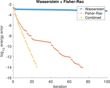
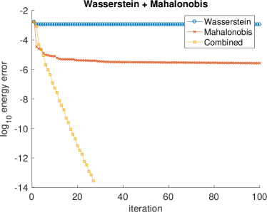
(1)	(2)
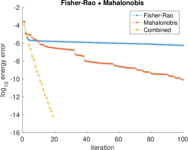
(3)	(4)

Figure 1. (1) Wasserstein plus Fisher-Rao terms tested with Wasserstein GD, Fisher-Rao GD, and the combined natural gradient. (2) Wasserstein plus Mahalanobis terms tested with Wasserstein GD, Mahalanobis GD, and the combined natural gradient. (3) Fisher-Rao plus Mahalanobis terms tested with Fisher-Rao GD, Mahalanobis GD, and the combined natural gradient. (4) Wasserstein plus Fisher-Rao plus Mahalanobis terms tested with Wasserstein GD, Fisher-Rao GD, Mahalanobis GD, and the combined natural gradient.

1. $(\alpha_{1},\alpha_{2},\alpha_{3})=(1,10^{-3},0)$, i.e., turning off the Mahalanobis term. The combined natural gradient converges much more rapidly compared to the Wasserstein GD and the Fisher-Rao GD.

2. $(\alpha_{1},\alpha_{2},\alpha_{3})=(1,0,10^{-4})$, i.e., turning off the Fisher-Rao term. The combined natural gradient converges much more rapidly compared to the Wasserstein GD and the Mahalanobis GD.

3. $(\alpha_{1},\alpha_{2},\alpha_{3})=(0,10^{-3},10^{-4})$, i.e., turning off the Wasserstein term. The combined natural gradient converges much more rapidly compared to the Fisher-Rao GD and the Mahalanobis GD.

4. $(\alpha_{1},\alpha_{2},\alpha_{3})=(1,10^{-3},10^{-4})$. The combined natural gradient converges much more rapidly compared to the Wasserstein GD, the Fisher-Rao GD, and the Mahalanobis GD.

3.2. 2D

Consider now the 2D domain $\Omega=[0,1]^{2}$ with periodic boundary condition. Among the three terms of the combined loss functional $E(p)=\alpha_{1}E_{1}(p)+\alpha_{2}E_{2}(p)+\alpha_{3}E_{3}(p)$, $E_{1}(p)$ is again chosen to be the weighted semi $H^{-1}$-norm

$$E_{1}(p)=\frac{1}{2}\lVert p-\mu\rVert_{\dot{H}^{-1}(\mu)}.$$

After discretization, it takes the following form

$$E_{1}(p)=\frac{1}{2}(p-\mu)^{\mathsf{T}}(D_{1}^{\mathsf{T}}\mu D_{1}+D_{2}^{\mathsf{T}}\mu D_{2})^{+}(p-\mu)$$

where $D_{1}$ and $D_{2}$ are the derivative operators in the first and the second directions. $E_{2}(p)$ is again the Kullback-Leibler divergence

$$E_{2}(p)=\sum_{s}p_{s}\log\frac{p_{s}}{\mu_{s}}.$$

Finally, $E_{3}(p)$ is given by

$$E_{3}(p)=\frac{1}{2}(p-\mu)^{\mathsf{T}}(-\Delta)(p-\mu)=\frac{1}{2}(p-\mu)^{\mathsf{T}}(D_{1}^{\mathsf{T}}D_{1}+D_{2}^{\mathsf{T}}D_{2})(p-\mu)$$

so $A=(-\Delta)$.

The domain is discretized with $n=64$ grid point in each direction. $\mu(s_{1},s_{2})\sim\exp(-V(s_{1},s_{2}))$ with $V(s_{1},s_{2})=\sin(4\pi s_{1})\sin(4\pi s_{2})$. The constant factors of the three terms are set to be $1$, $3\cdot 10^{-4}$, and $10^{-4}$ in order to balance the contribution from them so that no one dominates. We test with four different linear combinations, with the results summarized in Figure 2.

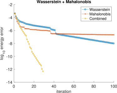
(1)	(2)
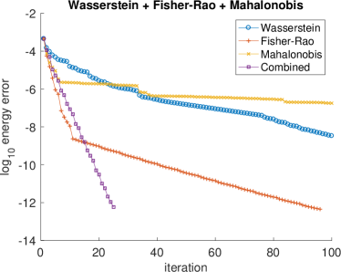
(3)	(4)

Figure 2. (1) Wasserstein plus Fisher-Rao terms tested with Wasserstein GD, Fisher-Rao GD, and the combined natural gradient. (2) Wasserstein plus Mahalanobis terms tested with Wasserstein GD, Mahalanobis GD, and the combined natural gradient. (3) Fisher-Rao plus Mahalanobis terms tested with Fisher-Rao GD, Mahalanobis GD, and the combined natural gradient. (4) Wasserstein plus Fisher-Rao plus Mahalanobis terms tested with Wasserstein GD, Fisher-Rao GD, Mahalanobis GD, and the combined natural gradient.

1. $(\alpha_{1},\alpha_{2},\alpha_{3})=(1,3\cdot 10^{-4},0)$, i.e., turning off the Mahalanobis term. The combined natural gradient converges much more rapidly compared to the Wasserstein GD and the Fisher-Rao GD.

2. $(\alpha_{1},\alpha_{2},\alpha_{3})=(1,0,10^{-4})$, i.e., turning off the Fisher-Rao term. The combined natural gradient converges much more rapidly compared to the Wasserstein GD and the Mahalanobis GD.

3. $(\alpha_{1},\alpha_{2},\alpha_{3})=(0,3\cdot 10^{-4},10^{-4})$, i.e., turning off the Wasserstein term. The combined natural gradient converges much more rapidly compared to the Fisher-Rao GD and the Mahalanobis GD.

4. $(\alpha_{1},\alpha_{2},\alpha_{3})=(1,3\cdot 10^{-4},10^{-4})$. The combined natural gradient converges much more rapidly compared to the Wasserstein GD, the Fisher-Rao GD, and the Mahalanobis GD.

4. Discussions

This note proposes a new natural gradient for minimizing combined loss functionals by using diagonal approximation in the wavelet basis. There are a few open questions. First, so far we have considered regular domains in one and two dimensions with periodic boundary condition. One direction is to extend this to more general domains using more sophisticated wavelet bases.

Second, we have assumed that the probability density $p$ is non-vanishing everywhere in deriving the interpolating natural gradient metric. It is an important question whether one can remove this condition in order to work with more general probability densities.

Third, the dynamics in the wavelet coefficients (5) enjoys a diagonal metric. It is tempting to ask whether it is possible to design a mirror descent algorithm. Due to the coupling between different wavelet coefficients in the metric computation $H_{1}Wc$ and $H_{2}Wc$, this seems quite difficult. An interesting observation is that the metric of the coarse scale wavelet coefficients is nearly independent of the values of the fine scale coefficients, while the metric of the fine scale ones depends heavily on the values of the coarse scale ones. This naturally brings the question of whether the combined metric (or even the Wasserstein metric) has an approximate multiscale structure. The wavelet analysis has played an important role understanding the earth mover distance metric $W_{1}$ [indyk2003fast, shirdhonkar2008approximate]. It seems that it might also play a role in understanding the $W_{2}$ metric.