Present address: ]Department of Chemistry and Chemical Biology, Harvard University, 12 Oxford St, Cambridge MA 02138

Present address: ]Honeywell Quantum Solutions, 303 S. Technology Ct., Broomfield, CO 80021, USA

Present address: ]Institute for Quantum Electronics, ETH Zürich, Otto-Stern-Weg 1, 8093 Zürich, Switzerland

Present address: ]National Institute of Standards and Technology, 325 Broadway, Boulder, Colorado 80305, USA

Present address: ]Department of Physics and Astronomy, University of Nevada, Las Vegas, Las Vegas, NV 89154

Experimental constraint on axion-like particle coupling over seven orders of magnitude in mass

Abstract

We use our recent electric dipole moment (EDM) measurement data to constrain the possibility that the HfF⁺ EDM oscillates in time due to interactions with candidate dark matter axion-like particles (ALPs). We employ a Bayesian analysis method which accounts for both the look-elsewhere effect and the uncertainties associated with stochastic density fluctuations in the ALP field. We find no evidence of an oscillating EDM over a range spanning from 27 nHz to 400 mHz, and we use this result to constrain the ALP-gluon coupling over the mass range $10^{-22}-10^{-15}$ eV. This is the first laboratory constraint on the ALP-gluon coupling in the $10^{-17}-10^{-15}$ eV range, and the first laboratory constraint to properly account for the stochastic nature of the ALP field.

A measurement of the permanent electric dipole moment of the electron (eEDM, $d_{e}$) well above the standard model prediction of $|d_{e}|\leq 10^{-38}e\,\textrm{cm}$ would be evidence of new physics [1, 2, 3, 4, 5]. The search for permanent EDMs of fundamental particles was launched by Purcell and Ramsey in the 1950s [6, 7], but it was not until recently that physicists began to consider the possibility of time-varying EDMs inspired in large part by hypothetical axion-like particles (ALPs) [8, 9, 10, 11, 12, 13]. Coupling to ALPs can cause EDMs of paramagnetic atoms and molecules to vary, due to variations in $d_{e}$ or the scalar-pseudoscalar nucleon-electron coupling $C_{S}$. In this paper, we extend our analysis of the EDM data we collected in 2016 and 2017 [14] to place a limit on the possibility that $C_{S}$ oscillates in time. This allows us to put a constraint on the hypothetical ALP-gluon coupling over seven orders of magnitude in mass.

Dark matter is one of the largest unsolved mysteries in modern physics: the microscopic nature of 84% of our universe’s cosmic matter density remains inscrutable [15]. A family of candidate dark matter particles called axion-like particles are pseudoscalar fields favored for their potential role in solving problems such as the strong CP problem, baryogenesis, the cosmological constant, and small-scale cosmic structure formation [16]. ALPs can be anything from the QCD axion [17, 18, 19, 20] to ultralight axions from string theory [21], with different models favouring different mass ranges [22, 23, 24, 16, 25, 26]. In this paper, we will consider ultralight spin-0 bosonic fields whose mass $m_{a}$ can range from $10^{-24}-10^{1}$ eV (or $10^{-10}-10^{15}$ Hz) [26]. ALPs in the low end of this mass range would solve some issues pertaining to small scale structure raised by astrophysical results [25, 27, 16, 28].

Ultralight dark matter particles such as these must be bosonic: the observed matter density can’t be reproduced with light fermions because their Fermi velocity would exceed the galactic escape velocity. The resulting field has high mode occupation, is well described classically as a wave, and oscillates primarily at the Compton frequency $\nu=m_{a}c^{2}/h$. Astrophysical observations tell us that a quasi-Maxwellian dark matter velocity distribution would have, near earth, a dispersion of $\delta v\sim 10^{-3}c$, which in turn leads to a coherence for the dark matter (DM) wave of about $10^{6}$ cycles [29]. This finite linewidth ultimately limits the sensitivity of any experiment whose total observation time approaches or exceeds the coherence time.

Several distinct couplings to ALP fields can result in an oscillating CP-odd quantity such as $d_{e}$ or $C_{S}$, which amounts to an oscillating molecular EDM signal in our data. The most straightforward effect is the derivative coupling of the ALP field to the pseudovector electron current operator — in other words, a direct coupling between ALP and electron. Unfortunately, in an atomic or molecular system the observable effect scales linearly with $m_{a}$, leading to a large suppression for the mass range we explore [13]. A second potential coupling is from the ALP-induced modification of the electron-nucleon Coulomb interaction [12]. Regrettably, the nature of this effect has not been elucidated in detail, but it is also expected to scale linearly with $m_{a}$ [30]. Finally, there are two distinct effects due to the coupling of ALPs to gluons. The first leads to a partially screened nuclear EDM which would be enhanced in polar molecules but scales linearly with $m_{a}$, which again is problematic in the mass range we probe [31]. The second effect will result in an oscillating $C_{S}$ and this is independent of $m_{a}$ [32, 33, 34]. In this paper, we use the hypothesized oscillation in $C_{S}$ to constrain the ALP-gluon coupling.

To understand the analysis discussed herein, the reader should be familiar with a few key details from the original measurement. Complete details can be found in [14] and references therein. The heart of our experiment is an electron spin precession measurement of ¹⁸⁰Hf¹⁹F⁺ molecular ions confined in a radio-frequency Paul trap and polarized in a rotating bias field to extract the relativistically-enhanced CP-violating energy shift $2hW_{S}C_{S}$ between the stretched and oriented $m_{F}\Omega$ Stark sublevels [35]. The molecule-specific structure constant $W_{S}=20.4$ kHz [36], $h$ is Planck’s constant, and we assume for the remainder of this paper that $d_{e}$ is zero.

In an individual run (or shot) of the experimental procedure, many HfF⁺ ions are loaded into an ion trap, and the internal quantum population is concentrated into one of four internal sublevels by means of pulses of polarized light. The energy difference between two sublevels is interrogated with Ramsey spectroscopy [14]. The population is put into a superposition of two levels by means of a coherent mixing pulse, and then allowed to coherently evolve for a variable time $t_{R}$, before a second coherent pulse remixes the two levels. The resulting population in a sublevel is destructively read out by means of final series of laser pulses, which induce photodissociation of HfF⁺ ions into Hf⁺ ions with a probability proportional to the population in the interrogated sublevel. The procedure requires about one second and the ion dissociation signal has a component which oscillates with $t_{R}$ as $\cos(2\pi f_{R}t_{R})$, where $f_{R}$ is proportional to the energy difference (averaged over the $\sim$0.5 second coherent evolution time $t_{R}$) between the $m_{F}=\pm 3/2$ magnetic sublevels of a given Stark level. There are multiple contributions to $f_{R}$, including Zeeman shifts and Berry’s phase shifts. Over the course of a block of data, comprising 1536 experimental shots, we chop the direction of the ambient magnetic field, the rotation direction of the bias field, and the internal Stark level probed, and for each of these eight different experimental configurations we sample multiple Ramsey times, in order to extract $f_{R}$ under eight different laboratory conditions. A certain linear combination of all the various $f_{R}$ measurements isolates, to first order, the CP-violating contribution to the energy difference, $f^{C_{S}}=2W_{S}C_{S}$, where in this case we are sensitive to the average value of $C_{S}$ during the $\sim$22 minutes required to collect a block of data.

To probe for a possible time-variation in $C_{S}$, our analysis is broken into two parts: ‘low frequency’ (27 nHz – 126 $\mu$Hz), corresponding to hypothesized variations in $W_{S}$ with periods shorter than the overall 14 month span of data collection but still long compared to the duration of a block, and ‘high frequency’ (126 $\mu$Hz – 400 mHz), corresponding to periods shorter than our most sensitive period of data collection ($\sim$11 days) but still long compared to the duration of a shot ($\sim$1 second)[37, 38].

The low-frequency Least Squares Spectral Analysis (LSSA) is straightforward: we take the bottom-line results for each of our 842 blocks of data ($f^{C_{Si}}$, $\sigma_{i}$, $T_{i}$), where $T_{i}$ is the time in seconds at which the $i^{th}$ block was collected, relative to the center of our data set (at 00:17 UTC, Aug 16, 2016), and $\sigma_{i}$ is the standard error on $f^{C_{Si}}$. Then for each hypothesized ALP frequency $\nu_{i}=\omega/(2\pi)$ in a set of equally spaced trial frequencies in the low-frequency range, we assume

$$f^{C_{S}}(T)=A\cos(\omega T)+B\sin(\omega T),$$ (1)

and do a weighted least-squares fit [38] to extract our best values $A_{0}(\nu)$ and $B_{0}(\nu)$.

For the high-frequency LSSA analysis we want to resolve hypothesized changes in $f^{C_{S}}$ that occur over the time scales $\leq$ 22 minutes (the time required to collect a block), so we disaggregate each block into its 1536 component measurements: the number of dissociated ions N measured for each of the shots that make up a block. The expected value for N for each shot is an oscillatory function of the Ramsey time $t_{R}$. The frequency of the oscillation in $t_{R}$ is modulated because a component of $f_{R}$ is proportional to $C_{S}$, hypothesized to be an oscillatory function of $T_{i}$, and the sign of the modulation amplitude depends on the sign of the bias magnetic field applied for that shot, and on the Stark doublet selected for probing for that shot. The least-squares fitting routine is correspondingly more complicated [38] but at the end of the day we again extract best-fit values $A_{0}(\nu)$ and $B_{0}(\nu)$ for each hypothesized value of the ALP oscillation frequency $\nu$ in the equally spaced grid of trial frequencies across the high-frequency range.

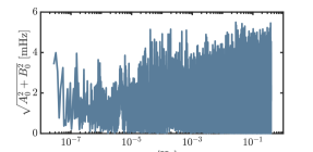
Figure 1: Least-squares spectral analysis of our EDM data.

Combining the two analyses, we obtain a measure of the best fit oscillation amplitude over seven orders of magnitude (Figure 1). Now we can ask: to what extent do our fit values convince us that $C_{S}$ is actually oscillating, given experimental noise and the look-elsewhere effect [39]? To answer this question we used the Bayesian Power Measured (BPM) analysis framework developed by Palken et al. [40].

The essence of the BPM framework is a comparison between the probability of measuring a given oscillation amplitude assuming the existence of an ALP with a specified mass and coupling and the probability of measuring the same amplitude assuming it doesn’t exist. This means we need probability distributions for both cases at each frequency $\nu$, which we can evaluate at the actual measured values $A_{0},B_{0}$. For the case where ALPs do not exist, we get the distributions by generating simulated data which by construction has no coherent $C_{S}$ oscillation in it. For the low frequency data we generate a single point of ‘noise’ at each acquisition time in the real dataset. Each point of noise is drawn from a Gaussian distribution with mean of zero and a variance which matches that of the real dataset. For the high frequency analysis we randomly shuffle the timestamps of the individual Ramsey measurements in such a manner as to effectively erase any coherent oscillation which may be present in the $C_{S}$ channel while preserving both the basic structure of the data (including the general coherent oscillation present in each Ramsey dataset) and the technical noise (see [38] for more details).

Once we have this simulated data we perform LSSA on it to get best fit values for $A,B$ at each frequency $\nu$ of interest. We repeat this process 1000 times. The resultant distribution of $A_{0},B_{0}$ at each frequency $\nu$ represents what we would expect to find in a universe where ALPs do not exist. Each distribution is bivariate normal with some rotation angle. We rotate each distribution into the primary axes $A^{\prime},B^{\prime}$ where the variance of the distribution is maximized along $A^{\prime}$ and minimized along $B^{\prime}$, to define the no-ALP distribution:

$$\mathcal{N}=\frac{1}{2\pi\sigma_{A^{\prime}}\sigma_{B^{\prime}}}e^{-\frac{1}{2}(\frac{A^{\prime 2}}{\sigma_{A^{\prime}}^{2}}+\frac{B^{\prime 2}}{\sigma_{B^{\prime}}^{2}})}.$$ (2)

We still need to determine the probability distributions in the case that ALPs do exist. Note that $A^{\prime}$ and $B^{\prime}$ are still random variables in this case due to the stochastic nature of the ALP field: different spatio-temporal modes of the field interfere with each other (the ALP field at any point in space is a sum over many contributions with random phases), so the field amplitude is stochastic over timescales longer than the coherence time [41, 42]. Except at the very high end of our analysis range, the ALP coherence time is much larger than the duration of our measurement, so we resolve only a single mode of the ALP field. In this limit the local ALP field may be written in the form

$$a(T)=\alpha\sqrt{\rho_{\rm DM}}/m_{a}\cos(\omega T+\phi),$$ (3)

where we take the mean local dark matter density $\rho_{\rm DM}$ to be $0.4\ \textrm{GeV/cm}^{3}$ [43], $\omega$ includes a small contribution from the ALP kinetic energy, $\phi\in[0,2\pi)$ is a uniform-distributed random variable, and $\alpha\geq 0$ is a Rayleigh-distributed random variable: $P(\alpha)=\alpha e^{-\alpha^{2}/2}$. The modifications to our analysis due to the decoherence of the ALP field are discussed in our Supplemental Material [38], otherwise we assume $\alpha$ and $\phi$ are constant over the entire data collection time. The oscillating $C_{S}$ term in the Ramsey fringe frequency is then written as

$$f^{C_{S}}(T)=2W_{S}\eta C_{G}/f_{a}a(T),$$ (4)

where $C_{G}/f_{a}$ is the ALP-gluon coupling (see [38] for alternative parameterizations) and $\eta\approx 0.03$ is a coefficient relating $C_{S}$ induced in a generic heavy nucleus to the QCD theta angle [32, 44]. The quadrature amplitudes of the ALP signal are then

$$A^{\prime} =2W_{S}\eta C_{G}/f_{a}\alpha\sqrt{\rho_{\rm DM}}/m_{a}\cos(\phi)$$ (5)

$$B^{\prime} =-2W_{S}\eta C_{G}/f_{a}\alpha\sqrt{\rho_{\rm DM}}/m_{a}\sin(\phi).$$

As mentioned earlier, $A^{\prime}$ and $B^{\prime}$ must still be treated as random variables even in the absence of noise; the fact that $\alpha$ is Rayleigh-distributed implies that $A^{\prime}$ and $B^{\prime}$ are each Gaussian distributed with mean zero and variance

$$\sigma_{X}^{2}=(2W_{S}\eta C_{G}/f_{a}\sqrt{\rho_{\rm DM}}/m_{a})^{2}.$$ (6)

The equal quadrature variances reflect our ignorance of the local phase of the ALP field oscillations. The fact that $A^{\prime}$ and $B^{\prime}$ can simultaneously be small reflects the possibility that the earth may have been near a null in ALP density during our data collection time. We can now construct the expected ‘ALP distribution’ by adding the variance $\sigma_{X}^{2}$ to our no-ALP variances (the no-ALP variances characterize the experimental noise). This defines a new bivariate normal distribution

$$\mathcal{X}=\frac{1}{2\pi\sigma_{AX}\sigma_{BX}}e^{-\frac{1}{2}(\frac{A^{\prime 2}}{\sigma_{AX}^{2}}+\frac{B^{\prime 2}}{\sigma_{BX}^{2}})},$$ (7)

which we call our ‘ALP distribution’. Here, $\sigma_{AX}^{2}=\sigma_{A^{\prime}}^{2}+\zeta\sigma_{X}^{2}$ and $\sigma_{BX}^{2}=\sigma_{B^{\prime}}^{2}+\zeta\sigma_{X}^{2}$. We encapsulate sources of attenuation, including decoherence of the ALP field due to the finite linewidth, in the frequency-dependent factor $\zeta$ which we discuss in detail in the Supplemental Material [38].

Now we can compare probabilities for the ALP vs no-ALP case. For each hypothesized coupling strength $C_{G}/(f_{a}m_{a})$ and frequency $\nu$ of interest we take the ratio of the probability distributions $\mathcal{N}$ and $\mathcal{X}$ evaluated at our actual measured amplitudes $A_{0}^{\prime}$ and $B_{0}^{\prime}$:

$$U_{i}(\nu_{i},C_{G}/(f_{a}m_{a}))=\frac{\mathcal{X}(A_{0}^{\prime}(\nu_{i}),B_{0}^{\prime}(\nu_{i}),\nu_{i},C_{G}/(f_{a}m_{a}))}{\mathcal{N}(A_{0}^{\prime}(\nu_{i}),B_{0}^{\prime}(\nu_{i}),\nu_{i})},$$ (8)

which we call the prior update: the number $U_{i}$ is a multiplicative factor which, when multiplied with our logarithmically-uniform priors, updates our prior belief to our post-experimental (or posterior) belief (see Figure 2). Note the prior update is equal to the Bayes factor in the limit of very low priors, which is the the limit we are operating in. A 95% exclusion corresponds to the prior update dropping to 0.05 [40].

Figure 2: Bayesian power measured analysis of the EDM data. The grayscale matrix corresponds to a sub-aggregation of the prior updates $U$ over 100 logarithmically-spaced frequency bins. Darker shading on the logarithmic color scale corresponds to increased prior update, which can be interpreted as an increased belief in an ALP of given frequency $\nu$ at ALP-gluon coupling $C_{G}/(f_{a}m_{a})$. We use a blue line to indicate the 95% exclusion (which corresponds to the sub-aggregated update dropping to 0.05 [40]) for sub-aggregation over each decade. The corresponding greyscale matrix for this sub-aggregation is not shown. Finally, a dotted line corresponds to the aggregated exclusion over the full analysis range. The full un-aggregated matrix of $U$ values is available upon request.

So far, our analysis has not taken into account the look-elsewhere effect even though we are looking at more than $10^{6}$ frequencies. The colormap of $U$ in Figure 2 simply shows how our belief in the existence of ALPs has changed as a function of frequency and coupling. To account for the look-elsewhere effect one must move from a notion of how locally unlikely an event is to how globally unlikely it is. For example, what might seem unlikely in a single frequency bin (say, you only expect it to happen 1/1000 times) becomes rather unsurprising when you look in 1000 bins - in this case you should expect to see that event approximately once. Our local measure, the prior update, compares the probability distributions in each bin for the ALP vs the no-ALP case. To move to a global measure we generate the aggregate prior update:

$$\mathcal{U}(C_{G}/(f_{a}m_{a}))=\frac{\text{aggregate posterior}}{\text{aggregate prior}}=\frac{\sum_{i}U_{i}\epsilon/\nu_{i}}{\sum_{i}\epsilon/\nu_{i}},$$ (9)

where $\epsilon/\nu_{i}$ is our prior belief (for an ALP of frequency $\nu_{i}$), using logarithmically-uniform priors ($\epsilon$ being constant). The aggregate prior update correctly accounts for our logarithmic priors, which is necessary in broad searches like ours where the number of hypotheses tested varies strongly as a function of frequency but we expect the ALP is equally likely to be found in any frequency decade. Using equation 9 we can sub-aggregate over any subset of the analysis range and at any frequency we like, and any interested reader can do the same - the full un-aggregated matrix of $U$ values is available upon request. The aggregate prior update taken over the entire set of frequencies analyzed represents the fractional change in our belief that an ALP of a given coupling strength exists anywhere in the full analysis range, which appropriately accounts for the look-elsewhere effect. The aggregate prior update as a function of coupling strength is plotted in the Supplemental Material, where we also discuss our selection of the priors [38].

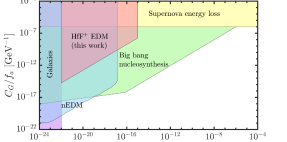
Figure 3: Astrophysical and laboratory limits on the ALP-gluon interaction. All limits assume that ALPs saturate the local dark matter content and we have taken the mean local dark matter density to be $0.4\ \textrm{GeV/cm}^{3}$ [43]. All constraints correspond to a 95% confidence level. The purple region embodies the constraint that the virial deBroglie wavelength is smaller than the size of a dwarf galaxy [26]. The blue region is the constraint derived from looking at neutron EDM oscillation [10]. The green region represents constraints from big bang nucleosynthesis [45], and the yellow region represents constraints from supernova energy loss bounds [46, 47]. The pink region is the constraint described in this work.

Our results yield no strong indication of a dark matter signal over the range $10^{-22}-10^{-15}$ eV, so we use the above procedure to exclude $C_{G}/f_{a}m_{a}>1.72\times 10^{16}$ GeV^-2 at 95% confidence. If we assume the density of the ALP field is held constant at its mean value, we can convert our exclusion back to frequency modulation amplitude in Hz via eq (3) and (4) which gives us an exclusion of 37 mHz. This is considerably less impressive-seeming than the limit of 1.2 mHz which we extracted from our original DC analysis [14]. This relaxation of the exclusion is an unavoidable consequence of correctly accounting for the stochastic nature of the ALP field and the look-elsewhere effect associated with setting a limit across seven orders of magnitude in frequency.

Our constraint on the ALP-gluon coupling $C_{G}/f_{a}$ is plotted in Figure 3 along with existing direct and indirect limits. Our results are the first laboratory constraints on the ALP-gluon coupling in the mass range $10^{-17}-10^{-15}$ eV.

The analysis techniques applied herein are general enough to apply to most time-series datastreams, and in particular will be applied to our next-generation EDM measurement which we expect to be about an order of magnitude more sensitive. More generally, the field of precision measurement is in a remarkable period of progress reminiscent of Moore’s Law, and we expect that analyses of this type will become more and more common. At the threshold of this era, we believe that it is critical to ask: how we can get the analysis of hypothesis exclusion right?

This is especially pertinent given that the existing frameworks and analyses already published have so far failed to account for important effects, such as the stochastic nature of the ALP field or the look-elsewhere effect. At least seven other dark matter exclusion publications have overestimated their exclusion by factors ranging from 3 to 10 in their failure to account for the stochasticity of the field [41]. To the best of our knowledge, the Bayesian analysis framework we have chosen here is optimal for this kind exclusion for several reasons: first, it easily incorporates the stochastic nature of the dark matter field, as well as the fact that the scale of the stochastic fluctuations changes as the measurement time approaches the coherence time of the dark matter field. In addition, this framework seamlessly accounts for the differential sensitivity of the the two quadratures of our measurement to the dark matter field, and can be easily scaled up to even higher dimensional parameter spaces. Finally, this framework correctly accounts for the the look-elsewhere effect with respect to exclusion [48]. Note that [10] in Figure 3 fails to account for the stochastic fluctuations in the ALP field, which could mean that their exclusion is overestimated by nearly an order of magnitude [41]. More generally, we appreciate how this framework preserves all the information in the signal compared to a threshold-based framework, which reduces the information in the signal to only ‘above’ or ‘below’ threshold.