Simulation of Brain Resection for Cavity Segmentation Using Self-Supervised and Semi-Supervised Learning

Abstract

Resective surgery may be curative for drug-resistant focal epilepsy, but only 40% to 70% of patients achieve seizure freedom after surgery. Retrospective quantitative analysis could elucidate patterns in resected structures and patient outcomes to improve resective surgery. However, the resection cavity must first be segmented on the postoperative MR image. Convolutional neural networks (CNNs) are the state-of-the-art image segmentation technique, but require large amounts of annotated data for training. Annotation of medical images is a time-consuming process requiring highly-trained raters, and often suffering from high inter-rater variability. Self-supervised learning can be used to generate training instances from unlabeled data. We developed an algorithm to simulate resections on preoperative MR images. We curated a new dataset, EPISURG, comprising 431 postoperative and 269 preoperative MR images from 431 patients who underwent resective surgery. In addition to EPISURG, we used three public datasets comprising 1813 preoperative MR images for training. We trained a 3D CNN on artificially resected images created on the fly during training, using images from 1) EPISURG, 2) public datasets and 3) both. To evaluate trained models, we calculate Dice score (DSC) between model segmentations and 200 manual annotations performed by three human raters. The model trained on data with manual annotations obtained a median (interquartile range) DSC of 65.3 (30.6). The DSC of our best-performing model, trained with no manual annotations, is 81.7 (14.2). For comparison, inter-rater agreement between human annotators was 84.0 (9.9). We demonstrate a training method for CNNs using simulated resection cavities that can accurately segment real resection cavities, without manual annotations.

1 Introduction

Only 40% to 70% of patients with refractory focal epilepsy are seizure-free after resective surgery [12]. Retrospective studies relating clinical features and resected brain structures (such as amygdala or hippocampus) to surgical outcome may provide useful insight to identify and guide resection of the epileptogenic zone. To identify resected structures, first, the resection cavity must be segmented on the postoperative MR image. Then, a preoperative image with a corresponding brain parcellation can be registered to the postoperative MR image to identify resected structures.

In the context of brain resection, the cavity fills with cerebrospinal fluid (CSF) after surgery [26]. This causes an inherent uncertainty in resection cavity delineation when adjacent to sulci, ventricles, arachnoid cysts or oedemas, as there is no intensity gradient separating the structures. Moreover, brain shift can occur during surgery, causing regions outside the cavity to fill with CSF.

Decision trees have been used for brain cavity segmentation from $T_{2}$-weighted, FLAIR, and pre- and post-contrast $T_{1}$-weighted MRI in the context of glioblastoma surgery [16, 10]. Relatedly, some methods have simulated or segmented brain lesions to improve non-linear registration with missing correspondences. Brett et al. [1] propagated lesions manually segmented from pathological brain images to structurally normal brain images by registering images to a common template space. Removing the lesion from consideration when computing the similarity metric improved non-linear registration. Methods to directly compute missing correspondences during registration, which can give an estimate of the resection cavity, have been proposed [5, 3, 7]. Pezeshk et al. [21] trained a series of machine learning classifiers to detect lesions in chest CT scans. The dataset was augmented by propagating lesions from pathological lungs to healthy lung tissue, using Poisson blending. This data augmentation technique improved classification results for all machine learning techniques considered.

In traditional machine learning, data is represented by hand-crafted features which may not be optimal. In contrast, deep learning, which has been successfully applied to brain image segmentation [13, 15], implicitly computes a problem-specific feature representation. However, deep learning techniques rely on large annotated datasets for training. Annotated medical imaging datasets are often small due to the financial and time burden annotating the data, and the need for highly-trained raters. Self-supervised learning generates training instances using unlabeled data from a source domain to learn features that can be transferred to a target domain [11]. Semi-supervised learning uses labeled as well as unlabeled data to train models [8]. These techniques can be used to leverage unlabeled medical imaging data to improve training in instances where acquiring annotations is time-consuming or costly.

We present a fully-automatic algorithm to simulate resection cavities from preoperative $T_{1}$-weighted MR images, applied to self-supervised learning for brain resection cavity segmentation. We validate this approach by comparing models trained with and without manual annotations, using 200 annotations from three human raters on 133 postoperative MR images with lobectomy or lesionectomy (133 annotations to test models performance and 67 annotations to assess inter-rater variability).

2 Methods

2.1 Resection Simulation

We generate automatically a training instance $(\bm{X}_{R},\bm{Y}_{R})$ representing a resected brain $\bm{X}_{R}$ and its corresponding cavity segmentation $\bm{Y}_{R}$ from a preoperative image $\bm{X}$ using the following approach.

(a)

(b)

(c)

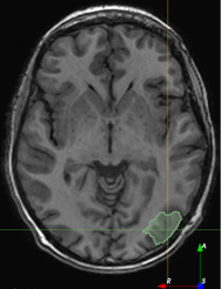
(d)

(e)

(f)

Figure 1: Resection simulation. (a) Sphere surface mesh before ($S$, green) and after ($S_{\delta}$, magenta) perturbation. $S$ and $S_{\delta}$ (top); intersection of $S$ and $S_{\delta}$ with a plane of the simplex noise volume, generated only for visualization purposes, with values between $-1$ (blue) and $1$ (red). Radial displacement is proportional to the noise at each vertex ${\bm{v}_{i}\in V}$ (b) Transformed mesh $S_{E}$ (c) Resectable hemisphere mask $\bm{M}_{R}$ (d) Simulated resection label $\bm{Y}_{R}$ (e) Simulated resected image $\bm{X}_{R}$ (f) Original image $\bm{X}$.

2.1.1 Resection Label

A geodesic polyhedron with frequency $f$ is generated by subdividing the edges of an icosahedron $f$ times and projecting each vertex onto a parametric sphere with unit radius. This polyhedron models a spherical surface $S=\{V,F\}$ with vertices $V=\left\{\bm{v}_{i}\in\mathbb{R}^{3}\right\}_{i=1}^{n_{V}}$ and faces $F=\left\{\bm{f}_{k}\right\}_{k=1}^{n_{F}}$. Each face $\bm{f}_{k}=\{i_{1}^{k},i_{2}^{k},i_{3}^{k}\}$ is defined as a sequence of three non-repeated vertex indices.

$S$ is perturbed with simplex noise [20], a smooth noise generated by interpolating pseudorandom gradients defined on a multidimensional simplicial grid. Simplex noise was selected as it is often used to simulate natural-looking textures or terrains. The noise at point $\bm{p}\in\mathbb{R}^{3}$ is computed as a weighted sum of the noise contribution of $\omega$ different octaves, with weights $\gamma^{n-1}:n\in\left\{1,2,\dots,\omega\right\}$ controlled by the persistence parameter $\gamma$. The displacement $\delta:\mathbb{R}^{3}\to[-1,1]$ is proportional to the noise function $\phi:\mathbb{R}^{3}\to[0,1]$:

$$\delta(\bm{p})=2\phi\left(\frac{\bm{p}+\bm{\mu}}{\zeta},\omega,\gamma\right)-1$$ (1)

where $\zeta$ is a scaling parameter to control smoothness and $\bm{\mu}$ is a shifting parameter that adds stochasticity (equivalent to a random number generator seed). Each vertex $\bm{v}_{i}\in V$ is displaced radially by:

$$\bm{v}_{\delta i}=\bm{v}_{i}+\delta(\bm{v}_{i})\frac{\overrightarrow{\bm{v}_{i}}}{\|\overrightarrow{\bm{v}_{i}}\|},\qquad\forall i\in\{1,2,\dots,n_{V}\}$$ (2)

to create a perturbed sphere $S_{\delta}=\{V_{\delta},F\}$ with vertices $V_{\delta}=\left\{\bm{v}_{\delta i}\right\}_{i=1}^{n_{V}}$ (Fig. 1a).

A series of transforms is applied to $S_{\delta}$ to modify its volume, shape and position. Let $T_{T}(\bm{p})$, $T_{S}(\bm{s})$ and $T_{R}(\bm{\theta})$ be translation, scaling and rotation transforms.

Perturbing $\bm{v}_{i}\in V$ shifts the centroid of $S_{\delta}$ off the origin. $S_{\delta}$ is recentered at the origin by applying the translation $T_{T}(\bm{-c})$ to each vertex, where ${\bm{c}=\frac{1}{n_{V}}\sum_{i=1}^{n_{V}}\bm{v}_{\delta i}}$ is the centroid of $S_{\delta}$.

Random rotations around each axis are applied to $S_{\delta}$ with the rotation matrix $T_{R}(\bm{\theta}_{r})=R_{x}(\theta_{x})\circ R_{y}(\theta_{y})\circ R_{z}(\theta_{z})$, where $\circ$ indicates a transform composition, $R_{i}(\theta_{i})$ is a rotation of $\theta_{i}$ radians around axis $i$, and $\theta_{i}\sim\mathcal{U}(0,2\pi)$.

A scaling transform $T_{S}(\bm{r})$ is applied to $S_{\delta}$, where $(r_{1},r_{2},r_{3})=\bm{r}$ are the semi-axes of an ellipsoid with volume $v$ modeling the cavity shape. The semi-axes are computed as $r_{1}=r$, $r_{2}=\lambda r$ and $r_{3}=r/\lambda$, where $r=(3v/4)^{1/3}$ and $\lambda$ controls the semi-axes length ratios.

$S_{\delta}$ is translated such that it is centered at a voxel in the cortical gray matter as follows. A $T_{1}$-weighted MR image is defined as $\bm{I}_{MRI}:\Omega\to\mathbb{R}$, where $\Omega\in\mathbb{R}^{3}$. A full brain parcellation $\bm{G}:\Omega\to Z$ is generated for $\bm{I}_{MRI}$ using geodesical information flows [2], where $Z$ is the set of segmented brain structures. A cortical gray matter mask $\bm{M}_{GM}^{h}:\Omega\to\{0,1\}$ of hemisphere $h$ is extracted from $\bm{G}$, where $h$ is randomly chosen from $H=\{\text{left},\text{right}\}$ with equal probability. A random gray matter voxel $\bm{g}\in\Omega$ is selected such that $\bm{M}_{GM_{h}}(\bm{g})=1$.

The transforms are composed as ${T_{E}=T_{T}(\bm{g})\circ T_{S}(\bm{r})\circ T_{R}(\bm{\theta}_{r})\circ T_{T}(-\bm{c})}$ and applied to $S_{\delta}$ to obtain the resection surface $S_{E}=T_{E}\circ S_{\delta}$. A mask ${\bm{M}_{E}:\Omega\to\{0,1\}}$ is generated from $S_{E}$ such that $\bm{M}_{E}(\bm{p})=1$ for all $\bm{p}$ within the cavity and $\bm{M}_{E}(\bm{p})=0$ outside.

If $\bm{M}_{E}$ is used as the final mask, the resection might span both hemispheres or include non-realistic tissues such as bone or scalp (Fig. 1b). To eliminate this unrealistic scenario, a ‘resectable hemisphere mask’ is generated from the parcellation as $\bm{M}_{R}(\bm{p})=1$ if ${\bm{G}(\bm{p})\neq\{\bm{M}_{BG},\bm{M}_{B},\bm{M}_{C},\bm{M}_{\hat{H}}\}}$ and $0$ otherwise, where $\bm{M}_{BG}$, $\bm{M}_{B}$, $\bm{M}_{C}$ and $\bm{M}_{\hat{H}}$ are the sets of labels in $Z$ corresponding to the background, brainstem, cerebellum and contralateral hemisphere, respectively. $\bm{M}_{R}$ is smoothed using a series of binary morphological operations (Fig. 1c). The final resection label used for training is $\bm{Y}_{R}(\bm{p})=\bm{M}_{E}(\bm{p})\bm{M}_{R}(\bm{p})$ (Fig. 1d).

2.1.2 Resected Image

To mimic partial volume effects near cavity boundaries, a Gaussian filter is applied to $\bm{M}_{R}(\bm{p})$ to smooth the alpha channel ${\bm{A}:\Omega\to[0,1]}$, defined as $\bm{A}(\bm{p})=\bm{M}_{R}(\bm{p})*\bm{G}_{\mathcal{N}}(\bm{\sigma}),\forall\bm{p}\in\Omega,$ where $*$ is the convolution operator and $\bm{G}_{\mathcal{N}}(\bm{\sigma}_{\bm{A}})$ is a Gaussian kernel with standard deviations $\bm{\sigma}_{\bm{A}}=(\sigma_{x},\sigma_{y},\sigma_{z})$.

To generate a realistic CSF texture, we create a ventricle mask ${\bm{M}_{V}:\Omega\to\{0,1\}}$ from $\bm{G}$, such that $\bm{M}_{V}(\bm{p})=1$ for all $\bm{p}$ within the ventricles and $\bm{M}_{V}(\bm{p})=0$ outside. Intensity values within ventricles are assumed to have a normal distribution [9] with a mean $\mu_{CSF}$ and standard deviation $\sigma_{CSF}$ calculated from voxel intensity values in $\bm{I}_{MRI}(\bm{p}):\forall\bm{p}\in\Omega,\bm{M}_{V}(\bm{p})=1$. A CSF-like image ${\bm{I}_{CSF}:\Omega\to\mathbb{R}}$ is then generated as $\bm{I}_{CSF}(\bm{p})\sim\mathcal{N}(\mu_{CSF},\sigma_{CSF}),\forall\bm{p}\in\Omega$, and the resected image (Fig. 1e) is the convex combination:

$$\bm{X}_{R}(\bm{p})=\bm{A}(\bm{p})\bm{I}_{CSF}(\bm{p}),+\left[1-\bm{A}(\bm{p})\right]\bm{I}_{MRI}(\bm{p})\qquad\forall\bm{p}\in\Omega$$ (3)

2.2 Dataset Description

$T1$-weighted MR images were collected from publicly available datasets Information eXtraction from Images (IXI) (566), Alzheimer’s Disease Neuroimaging Initiative (ADNI) (467), and Open Access Series of Imaging Studies (OASIS) (780), for a total of 1813 images. EPISURG was obtained from patients with refractory focal epilepsy who underwent resective surgery at the National Hospital for Neurology and Neurosurgery (NHNN), London, United Kingdom. This was an analysis of anonymized data that had been previously acquired as a part of clinical care, so individual patient consent was not required. In total there were 431 patients with postoperative $T_{1}$-weighted MR images, 269 of which had a corresponding preoperative MR image. All images were registered to a common template space using NiftyReg [17].

Three human raters annotated a subset of the postoperative images in EPISURG. Rater A segmented the resection cavity in 133 images. These annotations were used to test the models. This set was randomly split into 10 subsets, where the distribution of resection types (e.g. temporal, frontal, etc.) in each subset is similar. To quantify inter-rater variability, Rater B annotated subsets 1 and 2 (34 images), and Rater C annotated subsets 1 and 3 (33 images).

2.3 Network Architecture and Implementation Details

We used the PyTorch deep learning framework, training with automatic mixed precision on two 32-GB TESLA V100 GPUs. We implemented a variant of 3D U-Net [6] using two downsampling and upsampling blocks, trilinear interpolation for the synthesis path, and 1/4 of the filters for each convolutional layer. This results in a model with 100 times fewer parameters than the original 3D U-Net, reducing overfitting and computational burden. We used dilated convolutions [4], starting with a dilation factor of one, then increased or decreased in steps of one after each downsampling or upsampling block, respectively. Batch normalization and PReLU activation functions followed each convolutional layer. Finally, a dropout layer with probability 0.5 was added before the output classifier . We used an Adam optimizer  [14] with an initial learning rate of $10^{-3}$ and weight decay of $10^{-5}$. Training occurred for 60 epochs, and the learning rate was divided by 10 every 20 epochs. A batch size of 8 (4 per GPU) was used for training. 90% of the images were used for training and 10% for validation.

We wrote and used TorchIO [19] to process volumes on the fly during training. The preprocessing and random augmentation transforms used were 1) simulated resection (see Section 2.1), 2) MRI k-space motion artifact [23], 3) histogram standardization [18], 4) MRI bias field artifact [25], 5) normalization to zero-mean and unit variance of the foreground voxels, computed using the intensity mean as a threshold [18], 6) Gaussian noise, 7) flipping in the left-right direction, 8) scaling and rotation, and 9) B-spline elastic deformation. The resection simulation was implemented as a TorchIO [19] transform and the code is available online.

The following parameters were used to generate simulated resections (see Section 2.1): $f=16$, $\omega=4$, $\gamma=0.5$, $\zeta=3$, $\bm{\mu}\sim\mathcal{U}(0,1000)$, $\lambda\sim\mathcal{U}(1,2)$, and ${\bm{\sigma}_{\bm{A}}\sim\mathcal{U}(0.5,1)}$. The ellipsoid volume $v$ is sampled from volumes of manually segmented cavities from Rater A (see Section 2.2).

3 Experiments and Results

We trained models with seven different dataset configurations to assess how simulated resection cavities impact model accuracy a) using datasets of similar size and scanner, b) using datasets of similar size and different scanner, c) using much larger datasets ($10\times$ increase) and d) combined with semi-supervised learning.

All overlap measurements are expressed as ‘median (interquartile range)’ Dice score (DSC) with respect to the 133 annotations obtained from Rater A. Quantitative results are shown in Fig. 2.

Differences in model performance were analyzed by a one-tailed Mann-Whitney $U$ test with a significance threshold of $\alpha=0.05$, with Bonferroni correction for the seven experiments evaluated $\left(\frac{\alpha}{7\times(7-1)}\approx 0.002\right)$.

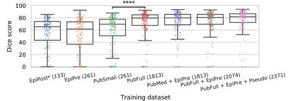
Figure 2: DSC values between manual annotations from Rater A and segmentations for models. Values in brackets indicate number of training subjects. Note that only the first model was trained with manual annotations. EpiPost: postoperative images in EPISURG with manual annotations (the asterisk * indicates fully supervised training with 10-fold cross-validation); EpiPre: preoperative images from subjects not contained in EpiPost); PubFull: public datasets; PubSmall, PubMed: subsets of PubFull; Pseudo: pseudo-labeled postoperative images in EPISURG.

3.1 Small Datasets

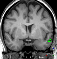
(a)

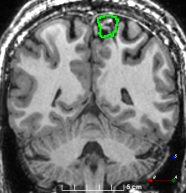
(b)

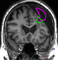
(c)

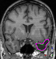
(d)

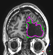
(e)

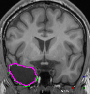
(f)

Figure 3: Manual labels from Rater A (green) and Rater D, the model trained with PubFull + EpiPre + Pseudo (magenta). Errors caused by a (a) small resection, (b) blood clot in cavity and (c) brain shift; segmentations corresponding to the (d) 50th, (e) 75th and (f) 100th percentiles giving a DSC of 81.7, 86.5 and 93.8, respectively.

We trained and tested on the 133 images annotated by Rater A, using 10-fold cross-validation, obtaining a DSC of 65.3 (30.6). We refer to this dataset as EpiPost. For all other models, we use data without manual annotations for training and EpiPost for testing.

EpiPre comprised 261 preoperative MR images from patients scanned at NHNN who underwent epilepsy surgery but are not in EpiPost. The model trained with EpiPre gave a DSC of 61.6 (36.6), which was not significantly different compared to training with EpiPost ($p=0.216$).

We trained a model using PubSmall, i.e. 261 images randomly chosen from the publicly available datasets. This model had a DSC of 69.5 (27.0).

Although there was a moderate increase in DSC, training with either EpiPre or PubSmall was not significantly superior compared to EpiPost after Bonferroni correction ($p=0.009$ and $p=0.035$, respectively).

3.2 Large Datasets

We trained a model using the full public dataset (PubFull, 1813 images), obtaining a DSC of 79.6 (17.3), which was significantly superior to PubSmall ($p\approx 10^{-8}$) and EpiPost ($p\approx 10^{-13}$). Adding EpiPre to PubFull for training did not significantly increase performance (${p=0.173}$), with a DSC of 80.5 (16.1).

For an additional training dataset, we created the PubMed dataset by replacing 261 images in PubFull with EpiPre. Training with PubMed + EpiPre was not significantly different compared to training with PubFull ($p=0.378$), with a DSC of 79.8 (17.1).

3.3 Semi-supervised Learning

We evaluated the ability of semi-supervised learning to improve model performance by generating pseudo-labels for all unlabeled postoperative images in EPISURG (297). Pseudo-labels were generated by inferring the resection cavity label using the model trained on PubFull and EpiPre. The pseudo-labels and corresponding postoperative images were combined to create the Pseudo dataset.

We trained a model using PubFull, EpiPre and Pseudo (2371 images), obtaining a DSC of 81.7 (14.2). Adding the pseudo-labels to PubFull and EpiPre did not significantly improve performance ($p=0.176$), indicating our semi-supervised learning approach provided no advantage. Predictions from this model are shown in Fig. 3.

3.4 Comparison to Inter-Rater Performance

We computed pairwise inter-rater agreement between the three human raters and the best performing model (trained with PubFull + EpiPre + Pseudo) as Rater D.

We computed consensus annotations between all pairs of raters using shape-based averaging [22]. DSCs between the segmentations from each rater and the consensuses generated by the other raters are reported in Fig. 4.

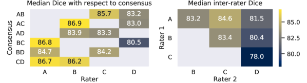
Figure 4: Left: median DSC between segmentations by a rater and consensuses from two other raters; right: median DSC between each rater segmentations. Rater D corresponds to the model trained with PubFull, EpiPre and Pseudo.

4 Discussion

We developed a method to simulate resection cavities on preoperative $T_{1}$-weighted MR images and performed extensive validation using datasets of different provenance and size. Our results demonstrate that, when the dataset is of a sufficient size, simulating resection from unlabeled data can provide more accurate segmentations compared to a smaller manually annotated dataset. We found that the most important factor for convolutional neural network (CNN) performance is using a training dataset of sufficient size (in this example, 1800+ samples). The inclusion of training samples from the same scanner or with pseudo-labels only marginally improved the model performance. However, we did not post-process the automatically-generated pseudo-labels, nor did we exclude predictions with higher uncertainty. Further improvements may be obtained by using more advanced semi-supervised learning techniques to appropriately select pseudo-labels to use for training.

Predictions errors are mostly due to 1) resection of size comparable to sulci (Fig. 6a), 2) unanticipated intensities, such as those caused by the presence of blood clots in the cavity (Fig. 6b), 3) brain shift (Fig. 6c) and 4) white matter hypointensities (Fig. 6e). Further work will involve using different internal and external cavity textures, carefully sampling the resection volume, simulating brain shift using biomechanical models, and quantifying epistemic and aleatoric segmentation uncertainty to better assess model performance [24].

The model has a lower inter-rater agreement score compared to between-human agreement values, however, this is well within the interquartile range of all the agreement values computed (Fig. 4). EPISURG will be made available, so that it may be used as a benchmark dataset for brain cavity segmentation.

Supplementary Material

Table 1: Datasets used for training. NHNN refers to National Hospital for Neurology and Neurosurgery. See Section 2.2 for more information about data provenance.

Name	Subjects	Source	Type	Annotations
EpiPost	133	NHNN	Postoperative	Yes
EpiPre	261	NHNN	Preoperative	No
Pseudo	297	NHNN	Postoperative	No
PubSmall	261	Public	Preoperative	No
PubMed	1552	Public	Preoperative	No
PubFull	1813	Public	Preoperative	No

Table 2: DSC values between manual annotations from Rater A and models segmentations, as shown in Fig. 2. Note that only the first model was trained with manual annotations. EpiPost: postoperative scans in EPISURG with manual annotations (* indicates fully-supervised training with 10-fold cross-validation); EpiPre: preoperative scans from subjects not contained in EpiPost); PubFull: public datasets; PubSmall, PubMed: subsets of PubFull; Pseudo: pseudo-labeled postoperative scans in EPISURG.

Training dataset	Subjects	Annotations	Dice score
EpiPost*	133	Yes	65.3 (30.6)
EpiPre	261	No	61.6 (36.6)
PubSmall	261	No	69.5 (27.0)
PubFull	1813	No	79.6 (17.3)
PubMed + EpiPre	1813	No	79.8 (17.1)
PubFull + EpiPre	2074	No	80.5 (16.1)
PubFull + EpiPre + Pseudo	2371	No	81.7 (14.2)

(a)

(b)

(c)

(d)

(e)

(f)

(g)

(h)

(i)

(j)

Figure 5: Resection simulations $\bm{X}_{R}$ generated using our method.

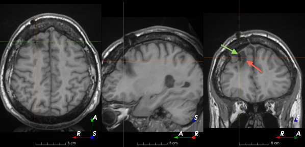
(a)

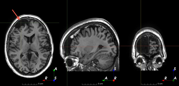
(b)

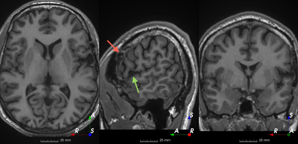
(c)

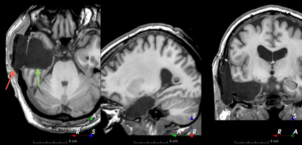
(d)

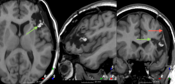
(e)

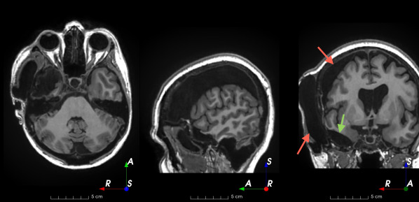
(f)

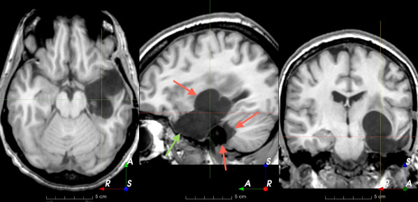
(g)

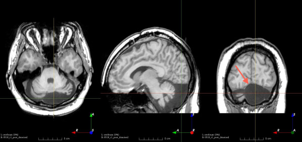
(h)

Figure 6: Examples of challenging images for cavity segmentation. (a) Small frontal lesionectomy surrounded by hypointense white matter (b) Brain shift after contralateral temporal lobectomy (not shown) (c) Small frontal lesionectomy near the Sylvian fissure (d) Lack of boundaries between oedema and resection cavity (e) Possible blood clot within the cavity (f) Brain shift, oedema and resection cavity (g) Arachnoid cyst and resection cavity (h) Cerebellar degeneration. Green annotations represent areas that correspond to resection cavities; red annotations represent areas that do not.

References

- [1] Brett, M., Leff, A.P., Rorden, C., Ashburner, J.: Spatial Normalization of Brain Images with Focal Lesions Using Cost Function Masking. NeuroImage 14(2), 486–500 (Aug 2001). https://doi.org/10.1006/nimg.2001.0845, http://www.sciencedirect.com/science/article/pii/S1053811901908456
- [2] Cardoso, M.J., Modat, M., Wolz, R., Melbourne, A., Cash, D., Rueckert, D., Ourselin, S.: Geodesic Information Flows: Spatially-Variant Graphs and Their Application to Segmentation and Fusion. IEEE Transactions on Medical Imaging 34(9), 1976–1988 (Sep 2015). https://doi.org/10.1109/TMI.2015.2418298
- [3] Chen, K., Derksen, A., Heldmann, S., Hallmann, M., Berkels, B.: Deformable Image Registration with Automatic Non-Correspondence Detection. In: Aujol, J.F., Nikolova, M., Papadakis, N. (eds.) Scale Space and Variational Methods in Computer Vision. pp. 360–371. Lecture Notes in Computer Science, Springer International Publishing, Cham (2015). https://doi.org/10.1007/978-3-319-18461-6_29
- [4] Chen, L.C., Papandreou, G., Kokkinos, I., Murphy, K., Yuille, A.L.: DeepLab: Semantic Image Segmentation with Deep Convolutional Nets, Atrous Convolution, and Fully Connected CRFs. arXiv:1606.00915 [cs] (May 2017), http://arxiv.org/abs/1606.00915, arXiv: 1606.00915
- [5] Chitphakdithai, N., Duncan, J.S.: Non-rigid Registration with Missing Correspondences in Preoperative and Postresection Brain Images. In: Jiang, T., Navab, N., Pluim, J.P.W., Viergever, M.A. (eds.) Medical Image Computing and Computer-Assisted Intervention – MICCAI 2010. pp. 367–374. Lecture Notes in Computer Science, Springer, Berlin, Heidelberg (2010). https://doi.org/10.1007/978-3-642-15705-9_45
- [6] Çiçek, Ö., Abdulkadir, A., Lienkamp, S.S., Brox, T., Ronneberger, O.: 3D U-Net: Learning Dense Volumetric Segmentation from Sparse Annotation. arXiv:1606.06650 [cs] (Jun 2016), http://arxiv.org/abs/1606.06650
- [7] Drobny, D., Carolus, H., Kabus, S., Modersitzki, J.: Handling Non-Corresponding Regions in Image Registration. In: Handels, H., Deserno, T.M., Meinzer, H.P., Tolxdorff, T. (eds.) Bildverarbeitung für die Medizin 2015. pp. 107–112. Informatik aktuell, Springer, Berlin, Heidelberg (2015). https://doi.org/10.1007/978-3-662-46224-9_20
- [8] van Engelen, J.E., Hoos, H.H.: A survey on semi-supervised learning. Machine Learning 109(2), 373–440 (Feb 2020). https://doi.org/10.1007/s10994-019-05855-6, https://doi.org/10.1007/s10994-019-05855-6
- [9] Gudbjartsson, H., Patz, S.: The Rician Distribution of Noisy MRI Data. Magnetic resonance in medicine 34(6), 910–914 (Dec 1995), https://www.ncbi.nlm.nih.gov/pmc/articles/PMC2254141/
- [10] Herrmann, E., Ermiş, E., Meier, R., Blatti-Moreno, M., Knecht, U.P., Aebersold, D.M., Manser, P., Mauricio, R.: Fully Automated Segmentation of the Brain Resection Cavity for Radiation Target Volume Definition in Glioblastoma Patients. International Journal of Radiation Oncology • Biology • Physics 102(3), S194 (Nov 2018). https://doi.org/10.1016/j.ijrobp.2018.07.087, https://www.redjournal.org/article/S0360-3016(18)31492-5/abstract
- [11] Jing, L., Tian, Y.: Self-supervised Visual Feature Learning with Deep Neural Networks: A Survey. arXiv:1902.06162 [cs] (Feb 2019), http://arxiv.org/abs/1902.06162, arXiv: 1902.06162
- [12] Jobst, B.C., Cascino, G.D.: Resective epilepsy surgery for drug-resistant focal epilepsy: a review. JAMA 313(3), 285–293 (Jan 2015). https://doi.org/10.1001/jama.2014.17426
- [13] Kamnitsas, K., Ledig, C., Newcombe, V.F.J., Simpson, J.P., Kane, A.D., Menon, D.K., Rueckert, D., Glocker, B.: Efficient Multi-Scale 3D CNN with Fully Connected CRF for Accurate Brain Lesion Segmentation. Medical Image Analysis 36, 61–78 (Feb 2017). https://doi.org/10.1016/j.media.2016.10.004, http://arxiv.org/abs/1603.05959, arXiv: 1603.05959
- [14] Kingma, D.P., Ba, J.: Adam: A Method for Stochastic Optimization. arXiv:1412.6980 [cs] (Dec 2014), http://arxiv.org/abs/1412.6980
- [15] Li, W., Wang, G., Fidon, L., Ourselin, S., Cardoso, M.J., Vercauteren, T.: On the Compactness, Efficiency, and Representation of 3D Convolutional Networks: Brain Parcellation as a Pretext Task. arXiv:1707.01992 10265, 348–360 (2017). https://doi.org/10.1007/978-3-319-59050-9_28, http://arxiv.org/abs/1707.01992
- [16] Meier, R., Porz, N., Knecht, U., Loosli, T., Schucht, P., Beck, J., Slotboom, J., Wiest, R., Reyes, M.: Automatic estimation of extent of resection and residual tumor volume of patients with glioblastoma. Journal of Neurosurgery 127(4), 798–806 (Oct 2017). https://doi.org/10.3171/2016.9.JNS16146
- [17] Modat, M., Cash, D.M., Daga, P., Winston, G.P., Duncan, J.S., Ourselin, S.: Global image registration using a symmetric block-matching approach. Journal of Medical Imaging 1(2) (Jul 2014). https://doi.org/10.1117/1.JMI.1.2.024003, https://www.ncbi.nlm.nih.gov/pmc/articles/PMC4478989/
- [18] Nyúl, L.G., Udupa, J.K., Zhang, X.: New variants of a method of MRI scale standardization. IEEE transactions on medical imaging 19(2), 143–150 (Feb 2000). https://doi.org/10.1109/42.836373
- [19] Pérez-García, F., Sparks, R., Ourselin, S.: TorchIO: a Python library for efficient loading, preprocessing, augmentation and patch-based sampling of medical images in deep learning. arXiv:2003.04696 [cs, eess, stat] (Mar 2020), http://arxiv.org/abs/2003.04696, arXiv: 2003.04696
- [20] Perlin, K.: Improving noise. ACM Transactions on Graphics (TOG) 21(3), 681–682 (Jul 2002). https://doi.org/10.1145/566654.566636
- [21] Pezeshk, A., Petrick, N., Chen, W., Sahiner, B.: Seamless lesion insertion for data augmentation in CAD training. IEEE transactions on medical imaging 36(4), 1005–1015 (Apr 2017). https://doi.org/10.1109/TMI.2016.2640180, https://www.ncbi.nlm.nih.gov/pmc/articles/PMC5509514/
- [22] Rohlfing, T., Maurer, C.R.: Shape-Based Averaging. IEEE Transactions on Image Processing 16(1), 153–161 (Jan 2007). https://doi.org/10.1109/TIP.2006.884936, conference Name: IEEE Transactions on Image Processing
- [23] Shaw, R., Sudre, C., Ourselin, S., Cardoso, M.J.: MRI k-Space Motion Artefact Augmentation: Model Robustness and Task-Specific Uncertainty. In: International Conference on Medical Imaging with Deep Learning. pp. 427–436 (May 2019), http://proceedings.mlr.press/v102/shaw19a.html
- [24] Shaw, R., Sudre, C.H., Ourselin, S., Cardoso, M.J.: A Heteroscedastic Uncertainty Model for Decoupling Sources of MRI Image Quality. arXiv:2001.11927 [cs, eess] (Jan 2020), http://arxiv.org/abs/2001.11927, arXiv: 2001.11927
- [25] Sudre, C.H., Cardoso, M.J., Ourselin, S.: Longitudinal segmentation of age-related white matter hyperintensities. Medical Image Analysis 38, 50–64 (May 2017). https://doi.org/10.1016/j.media.2017.02.007, http://www.sciencedirect.com/science/article/pii/S1361841517300257
- [26] Winterstein, M., Münter, M.W., Burkholder, I., Essig, M., Kauczor, H.U., Weber, M.A.: Partially resected gliomas: diagnostic performance of fluid-attenuated inversion recovery MR imaging for detection of progression. Radiology 254(3), 907–916 (Mar 2010). https://doi.org/10.1148/radiol09090893