Variational Autoencoding of PDE Inverse Problems

Abstract

Specifying a governing physical model in the presence of missing physics and recovering its parameters are two intertwined and fundamental problems in science. Modern machine learning allows one to circumvent these, via emulators and surrogates, but in doing so disregards prior knowledge and physical laws that are especially important for small data regimes, interpretability, and decision making. In this work we fold the mechanistic model into a flexible data-driven surrogate to arrive at a physically structured decoder network. This provides accelerated inference for the Bayesian inverse problem, and can act as a drop-in regulariser that encodes a-priori physical information. We employ the variational form of the PDE problem and introduce stochastic local approximations as a form of model based data augmentation. We demonstrate both the accuracy and increased computational efficiency of the framework on real world settings and structured spatial processes.

1 Introduction

Many important problems in science and engineering take the form of an inverse problem [42]. The typical task is to conduct inference over a parameter set indexing a mechanistic model, often presented as a partial differential equation (PDE), given observations. PDE based models allow one to specify and control complex interactions between inputs, ouputs and domain properties. Increasingly attention has switched to the potential of the forward map to act as a mechanistically inspired convolution, Fig. 1, with some of these features successfully exploited by [3, 40, 13, 44].

However, to leverage the full power of PDEs for inference, one must usually solve the forward problem, typically a nonlinear and expensive operation, making both exact and approximate posterior inference challenging. This has led to development of simulation based methods [10], gradient matching methods avoiding numerical integration [7, 19], and recently fast approximations to the likelihood [24] based on probabilistic numerics [30, 31]. Common to these approaches is an assumption that a parameterised mechanistic model is the correct model, however for many real world applications such certainty is difficult to countenance, necessitating methods which balance the structure of mechanistic models, with the flexibility to handle incomplete information.

Given these challenges it is natural to attempt to replace the forward map by some suitable family of approximating functions. Gaussian process (GP) surrogates offer a consistent probabilistic framework complete with uncertainty quantification [3, 33, 17], but are difficult to extend to nonlinear problems. Conversely, while deep generative methods easily handle nonlinear latent variables, it is harder to guarantee that the forward map is constrained by the underlying physics. Supervised deep learning methods have imposed this constraint by applying the PDE operator point-wise as an additional regularisation term [34, 39, 4, 32, 46] which, while allowing for efficient inference, can suffer when data is noisy [43, 8, 12]. Furthermore, extending these regularisation approaches to generative models is challenging, and while progress has been made on phyiscally constrained generative models [48], and structure preserving architectures [9, 45], demonstrating the flexible integration of more general networks with only partially known physics on real world problems remains challenging.

(a) Input source

(b) Transport vector field

(c) Output field

(e) Posterior

(d) Sensors

Figure 1: In the forward problem a noisy source (a), for example a pollutant, is convolved with some transporting vector field, (b), such as wind direction, to produce a smoothed output in a bounded domain (c). The Bayesian inverse problem uses information from a finite number of sensor locations (d) to recover the posterior distribution of the parameters of the forward map, in this instance the posterior direction vectors (e).

We address these open problems by utilising the weak-, or variational, form of the PDE problem as an inter-domain procedure [26] which augments learning with a fine-scale discretisation of the mechanistic model to perform regularisation on the dual problem. In Section 3 we show that a consistent description of our generative model begins from a dual-space relaxation of the mechanistic model which we embed inside a constrained optimisation problem. Unlike point-wise methods, we require global regularisation, necessitating the development in Sec. 4 of a local approximation, enabling substantial computational gains whilst maintaining accuracy on the inverse problem. We then empirically demonstrate the accuracy and efficiency of our method in Sec. 5 before concluding with a discussion and suggested future research

In summary, we demonstrate the embedding of partial physical knowledge into general decoders by relaxing a mechanistic model before using a constrained optimisation framework to produce a coherent generative structure supervised by a PDE inverse problem. To further enable regularisation by fine-scaled discretisations of the guiding PDE we also introduce a novel approximation over local meshes for efficient training. With these steps complete we show the resulting models’ ability to accelerate the classical BIP or to regularise general DL methods when prior physical knowledge is incomplete. We first assess the accuracy of our approach to the BIP using synthetic data; then demonstrate the applicability of our methods as physically informed plug-in enhancements for modelling real-world problems in heavy-metal contamination and water-resource management.

2 Bayesian inverse problems

The objective when solving a Bayesian inverse problem (BIP) [42] is to recover the posterior distribution of latent parameters, $\mathbf{z}$, which parameterise a forward map, $G[\mathbf{z}]$, from a spatial domain $\Omega\subset\mathbb{R}^{D}$ to observations. We denote the output from the forward map at location $\mathbf{x}$ by the field variable $u(\mathbf{x})=G[\mathbf{z}](\mathbf{x})$, here $G$ will arise as the solution to some mechanistic problem. The data for the inverse problem consists of a finite set of noisy observations $\mathbf{y}=\{y(\mathbf{x})_{n}\}_{n=1}^{N}$ observed at spatial locations $\mathbf{X}=\{\mathbf{x}_{n}\}_{n=1}^{N}$, where $\mathbf{x}_{n}\in\Omega\subset\mathbb{R}^{D}$, with the field variable acting as a deterministic link from the latent variables to observations in these locations through a likelihood $p(\mathbf{y}\mid\mathbf{u})$, and the target posterior is $p(\mathbf{z}\mid\mathbf{y})\propto p(\mathbf{y}\mid\mathbf{u}=G[\mathbf{z}](\mathbf{x}))p(\mathbf{z}).$ Inference up to an unknown normalising constant is standard, however the forward map is typically unavailable in closed form requiring expensive numerical methods. In this work we embed the BIP inside a constrained optimisation framework, following the optimisation view of Bayesian inference [47] that recovers the posterior as:

$$\qquad\operatorname*{arg\,min}_{q(\theta)\in\mathcal{P}(\Theta)}\quad\mathbb{E}_{q(\theta)}\left[-\log p(\mathbf{y}\mid\theta)\right]+\operatorname{KL}(q(\theta)\,\|\,p(\theta)),$$ (1)

where $\operatorname{KL}(q\,\|\,p)$ denotes the KL-divergence between distributions with densities $q$ and $p$, and $\mathcal{P}(\Theta)$ denotes the set of all distributions on the general parameter spaces $\theta\in\Theta$. Since the forward operator $G[\mathbf{z}]$ is deterministic we rewrite this formally as the equivalent constrained problem

$$\operatorname*{arg\,min}_{q(\mathbf{u},\mathbf{z})\in\mathcal{P}(V\times\mathcal{Z})}\quad \mathbb{E}_{q(\mathbf{u},\mathbf{z})}\left[-\log p(\mathbf{y}\mid\mathbf{u})\right]+\operatorname{KL}(q(\mathbf{u},\mathbf{z})\,\|\,p(\mathbf{u},\mathbf{z}))\quad\mbox{s. t. }p(\mathbf{u}\mid\mathbf{z})=\delta_{G[\mathbf{z}]}(\mathbf{u}),$$ (2)

where $\delta_{G(\mathbf{z})}(\mathbf{u})$ denotes the degenerate Dirac distribution centred on the deterministic solution and $V$ is a function space in which we assume the solution of the forward problem to exist, we refer to this as the space of trial functions [6]. In this work we initially relax the constrained problem (2), before showing that the structure can be recovered, allowing us to introduce variational methods respecting the generative structure of the model, but avoiding expensive evaluations of the forward map.

2.1 Partial differential equations and finite element discretisation

We focus on a particular instance of the BIP by examining forward maps which arise as the implicit solutions of PDEs. These models are a bedrock of modern science and engineering and they are presented in the form

$$\mathcal{L}[\mathbf{z}]u(\mathbf{x})=f(\mathbf{x})\mbox{ on }\Omega,\qquad u(\mathbf{x})=g(\mathbf{x})\mbox{ for }\mathbf{x}\in\partial\Omega,$$ (3)

where $\mathcal{L}[\mathbf{z}]$ is a differential operator parameterised by $\mathbf{z}$. The source, $f(\mathbf{x})$, represents domain wide inputs, while the boundary condition $\mathbf{g}(\mathbf{x})$ describes inputs acting only through the boundary, $\partial\Omega$. These models are complicated because (3) only defines the forward map implicitly, but can represent a diverse range of interesting dynamics. We can illustrate some of this richness by considering

$$\mathcal{L}[\mathbf{z}](\cdot)=-\nabla(a(\mathbf{x},\mathbf{z})\nabla(\cdot))+\boldsymbol{\tau}(\mathbf{x},\mathbf{z})\cdot\nabla(\cdot)$$ (4)

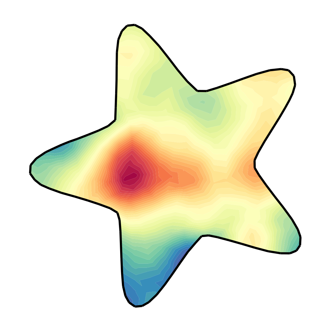
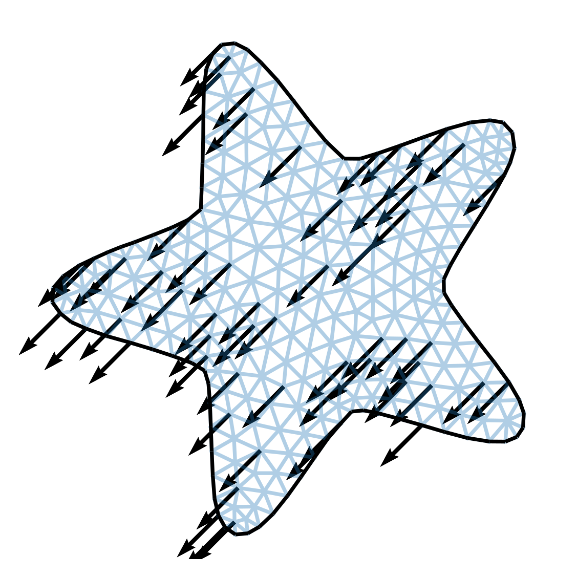
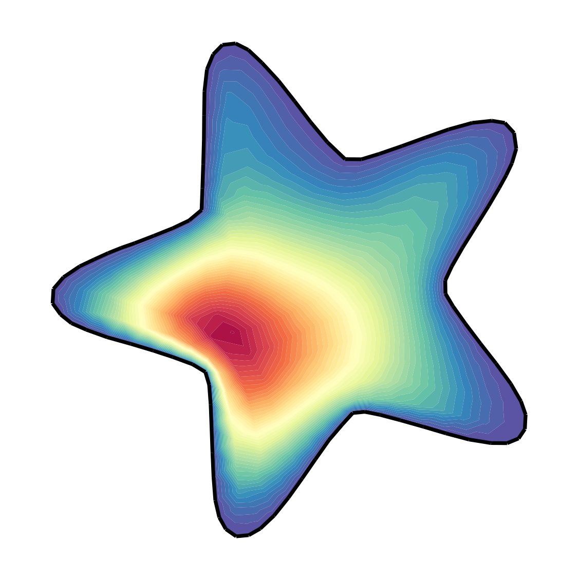
where $a(\mathbf{x})$ is the diffusion coefficient and $\boldsymbol{\tau}(\mathbf{x})$ is referred to as the transport vector field. We visualise the action of this operator in Fig. 1; in this instance we have an input source, for example pollutants represented in Fig. 1(a). The operator is parameterised by a transporting vector field $\boldsymbol{\tau}(\mathbf{x})$, such as the prevailing wind-direction, visualised in Fig. 1(b). The forward map can be viewed as a structured convolution, where pollutants are smoothed by the diffusion parameter $a(\mathbf{x})$, and transported by $\boldsymbol{\tau}(\mathbf{x})$ until they encounter the boundary. The solution $u(\mathbf{x})$ is represented in Fig. 1(c) in which we can clearly observe diffusion, transport and boundary effects.

Since the forward map is unavailable in closed form it becomes necessary to solve the PDE numerically, and the finite element method [5] (FEM) is a powerful method for doing so. To illustrate our review we shall discuss the Laplace operator, $\Delta=\nabla^{2}$, which leads to a special case of (4) as

$$-\Delta u(\mathbf{x})=f(\mathbf{x})\quad\mbox{ for }\mathbf{x}\in\Omega,\qquad u(\mathbf{x})=g(\mathbf{x})\quad\mbox{on }\partial\Omega.$$ (5)

To discretise one introduces a second function space, denoted $\hat{V}$, of test functions $v\in\hat{V}$, then multiplies the classical form (5) by $v$ and integrates to give the weak form of the classical problem

$$\int_{\Omega}\nabla u(\mathbf{x})\cdot\nabla v(\mathbf{x})d\mathbf{x}=\int_{\Omega}f(\mathbf{x})v(\mathbf{x})d\mathbf{x}-\int_{\partial\Omega}g(\mathbf{s})v(\mathbf{s})ds.$$ (6)

The variational problem is now: find solution $u\in V$ such that (6) holds for any test function $v\in\hat{V}$. To numerically implement this idea using the FEM method one decomposes $\Omega$ into a collection of disjoint elements, and specifies a finite dimensional set of basis functions $V=\mathrm{span}\{\phi_{i}\}$ and $\hat{V}=\mathrm{span}\{\hat{\phi}_{i}\}$ for the test and trial space respectively, which are completely determined by their values on the nodes $\{\bar{\mathbf{x}}_{j}\}_{j=1}^{N_{\text{nodes}}}$ of the mesh, see [35] for a full review of how this process is implemented. Having specified the basis, one searches for solutions with a representation $u_{n}(\mathbf{x})=\sum_{j=1}^{N}(\boldsymbol{\xi})^{u}_{j}\phi_{j}(\mathbf{x})$, where $\boldsymbol{\xi}^{u}\in\mathbb{R}^{N_{\text{nodes}}}$ are unknown coefficients. In matrix-vector notation we have $\mathbf{A}\boldsymbol{\xi}^{u}=\mathbf{f}$, where the stiffness matrix and load vector are given by

$$(\mathbf{A})_{ij}=\int_{\Omega}\nabla\phi_{j}(\mathbf{x})\cdot\nabla\hat{\phi}_{i}(\mathbf{x})dx\qquad(\mathbf{f})_{i}=\int_{\Omega}f(\mathbf{x})\hat{\phi}_{i}(\mathbf{x})dx-\int_{\partial\Omega}g(\mathbf{s})\hat{\phi_{i}}(\mathbf{s})d\mathbf{s}.$$ (7)

The use of nodal basis functions guarantees that $(\mathbf{A})_{ij}$ is zero whenever $\bar{\mathbf{x}}_{i}$ and $\bar{\mathbf{x}}_{j}$ are not in adjacent elements. Following the same procedure we can discretise (4) as

$$(\mathbf{L}[\mathbf{z}])_{ij}=\int_{\Omega}a(\mathbf{x},\mathbf{z})\nabla\phi_{j}(\mathbf{x})\cdot\nabla\hat{\phi}_{i}(\mathbf{x})dx+\int_{\Omega}\boldsymbol{\tau}(\mathbf{x},\mathbf{z})\cdot\nabla\phi_{j}(\mathbf{x})\hat{\phi}_{i}(\mathbf{x})dx.$$ (8)

We stress that while in principle these quadratures are defined over the entire domain, in practice owing to the sparsity of the nodal basis functions it is only necessary to perform this quadrature locally over adjacent elements. The solution of a PDE by the FEM therefore requires two steps

• [Assembly] The process of pushing forward the latent process $\mathbf{z}\mapsto\mathbf{L}[\mathbf{z}]$ through the quadrature (8). This is a $\mathcal{O}(N_{\text{elements}})$ embedding into a sparse matrix.

• [Solve] Inverting to solve $\boldsymbol{\xi}^{u}=\mathbf{L}[\mathbf{z}]^{-1}\mathbf{f}$. Direct application of this is $\mathcal{O}(N_{\text{nodes}}^{3})$.

To solve the BIP using the FEM it would be necessary to perform repeated calls to Assembly and Solve. In this work we shall only ever need to perform the cheap Assembly operation.

3 Structure-preserving Constrained VI

If we are going to circumvent the true forward map, but still encode the physical structure, then we must introduce an alternative means of ensuring the mechanism is embedded into the inferential process. In this section we show how we can do that through a VI framework which is augmented with the discretised weak-form that in turn encodes the mechanistic model. We first relax the inherent degeneracy of the objective problem (2), by introducing a one parameter family of approximating conditional densities, $p_{\epsilon}(\mathbf{u}\mid\mathbf{z})$. Our goal is to now specify such a $p_{\epsilon}$ so as to replace the original objective function by

$$F_{\epsilon}=\mathbb{E}_{q(\mathbf{u},\mathbf{z})}\left[-\log p(\mathbf{y}\mid\mathbf{u})\right]+\operatorname{KL}(q(\mathbf{z})\|p(\mathbf{z}))+\mathbb{E}_{q(\mathbf{z})}\left[\operatorname{KL}(q(\mathbf{u}\mid\mathbf{z})\|p_{\epsilon}(\mathbf{u}\mid\mathbf{z}))\right].$$ (9)

3.1 Relaxing the VI problem

One immediate way of achieving a relaxation that continues to respect the underlying PDE structure is to replace the original model (3) by

$$\mathcal{L}[\mathbf{z}]u(\mathbf{x})=f(\mathbf{x})+\epsilon w(\mathbf{x}),$$ (10)

where $w(\mathbf{x})$ is an independent Gaussian process perturbation, and $\epsilon>0$ is a scaling parameter. Using the FEM described in Section 2 to discretise we may write

$$p_{\epsilon}(\mathbf{u}\mid\mathbf{z})=\mathcal{N}(\mathbf{u}\mid\mathbf{L}[\mathbf{z}]^{-1}\mathbf{f},\epsilon^{2}(\mathbf{L}[\mathbf{z}]^{\top}\mathbf{D}\mathbf{L}[\mathbf{z}])^{-1})$$ (11)

where $\mathbf{D}$ is the precision matrix of the process $w(\mathbf{x})$ after projection onto the test space. However, it remains unclear how one should specify the covariance operator of $w(\mathbf{x})$. In fact we shall see below that in the limit this choice would not matter, but for practical implementations it does.

Our approach is motivated by [22] who note that if $u$ is an element of the Sobolev space $H_{0}^{1}$, then through the weak-form (6) a pair $(u,\mathbf{z})$ determines an element, which we denote by $\varphi_{u,\mathbf{z}}$, of the dual space $H^{-1}$. Ideally this should be small, so we place a Gaussian measure on $H^{-1}$ and then use the Riesz-Fréchet isomorphism and properties of the $H^{1}_{0}$ norm to construct a Gaussian measure

$$\exp\left\{\frac{-1}{2\epsilon^{2}}\|\varphi_{u,\mathbf{z}}\|^{2}_{H^{-1}}\right\}=\exp\left\{\frac{-1}{2\epsilon^{2}}\|(-\Delta^{-1})\varphi_{u,\mathbf{z}}\|^{2}_{H_{0}^{1}}\right\}=\exp\left\{\frac{-1}{2\epsilon^{2}}\langle\varphi_{u,\mathbf{z}},(-\Delta)^{-1}\varphi_{u,\mathbf{z}}\rangle_{L^{2}(\Omega)}\right\}$$

now replacing the dual space element $\varphi_{u,z}$ by the discretised weak-form $\mathbf{L}[\mathbf{z}]\mathbf{u}-\mathbf{f}$, and $(-\Delta)^{-1}$ by the inverse stiffness matrix, then we arrive at the density

$$p_{\epsilon}(\mathbf{u}\mid\mathbf{z})\propto\exp\left\{-\frac{1}{2\epsilon^{2}}\left(\mathbf{L}[\mathbf{z}]\mathbf{u}-\mathbf{f}\right)^{\top}\mathbf{A}^{-1}\left(\mathbf{L}[\mathbf{z}]\mathbf{u}-\mathbf{f}\right)\right\}$$

which after rearranging is precisely (11), with the precision matrix given by the stiffness matrix (7) from the FEM applied to the Poisson problem (5), that is $\mathbf{D}=\mathbf{A}^{-1}$. Intuitively, our relaxed model allows pairs $(u,\mathbf{z})$ which do not exactly satisfy the mechanistic model, and then penalises these deviations from exact solution pairs according to a Gaussian measure on the dual space, which we interpret as a space of “approximate mechanisms” While the idea of perturbing (10) to create a relaxed problem is not a new one, and is fundamental to emulator based methods [23], our dual-space relaxation leads to a somewhat counter-intuitive perturbing process. For instance, a natural choice of perturbation to (10) would be the stochastic PDEs considered in [27], characterised by dense covariances but sparse precisions allowing for efficient inference. Instead we are led to consider the reverse of this, and this will have important implications which we revisit in Sec. 4.

3.2 Re-constraining the VI problem

We now demonstrate how our approximation allow us to tackle the variational problem for the relaxation (9), and to examine the consequences of taking the limit $\epsilon\rightarrow 0$. Our variational family is distributions with conditionals of the form

$$q(\mathbf{u}\mid\mathbf{z})=\mathcal{N}(\mathbf{u}\mid\mu(\mathbf{x},\mathbf{z}),\epsilon^{2}(\mathbf{L}[\mathbf{z}]^{\top}\mathbf{A}^{-1}\mathbf{L}[\mathbf{z}])^{-1}),$$ (12)

where $\mu(\mathbf{x},\mathbf{z})$ is some free function of the spatial coordinates and latent parameters. We shall assume that the family of approximating functions has sufficient capacity to express the forward map, and therefore the exact conditional is contained within our family of approximating distributions. After integrating over $q(\mathbf{u}\mid\mathbf{z})$ then (9) becomes

$$F_{\epsilon}=\mathbb{E}_{\mathbf{u}\sim q(\mathbf{u},\mathbf{z})}\left[-\log p(\mathbf{y}\mid\mathbf{u})\right]+\operatorname{KL}(q(\mathbf{z})\|p(\mathbf{z}))+\frac{1}{2\epsilon^{2}}\mathbb{E}_{q(\mathbf{z})}\left[\left\|\mathbf{L}[\mathbf{z}]\mu(\mathbf{x},\mathbf{z})-\mathbf{f}\right\|_{\mathbf{A}}^{2}\right],$$ (13)

where $\|\mathbf{w}\|_{\mathbf{A}}$ denotes the quadratic form $\mathbf{w}^{\top}\mathbf{A}^{-1}\mathbf{w}$, note this has allowed us to avoid evaluating the covariance matrix in (12), which requires the prohibitive Solve. The first two terms of (13) are standard, and indeed are reminiscent of the decoding network of a variational autoencoder [25, 36] and we expand on that connection in the supplement. Less standard is the final term which provides strong mechanistic regularisation of the encoder network. To see this, let $\{\mathbf{z}_{i}\}_{i=1}^{M}$ be a collection of independent samples from $q(\mathbf{z})$, then we can obtain the MC approximation of (13) using

$$\mathbb{E}_{\mathbf{z}\sim q(\mathbf{z})}\left[\|\mathbf{L}[\mathbf{z}]\mu(\mathbf{x},\mathbf{z})-\mathbf{f}\|_{\mathbf{A}}^{2}\right]\approx\frac{1}{M}\sum_{i=1}^{M}\|\mathbf{L}[\mathbf{z}_{i}]\mu(\mathbf{x},\mathbf{z}_{i})-\mathbf{f}\|_{\mathbf{A}}^{2}.$$ (14)

Defining the scalar variable $r(\mathbf{z})\stackrel{{\scriptstyle\Delta}}{{=}}\|\mathbf{L}[\mathbf{z}]\mu(\mathbf{z})-\mathbf{f}\|_{\mathbf{A}}$, then we can approximate (13) as

$$F_{\epsilon}\approx\mathbb{E}_{\mathbf{u}\sim q(\mathbf{u},\mathbf{z})}\left[-\log p(\mathbf{y}\mid\mathbf{u})\right]+\operatorname{KL}(q(\mathbf{z})\|p(\mathbf{z}))+\frac{1}{2\epsilon^{2}M}\sum_{i=1}^{M}r(\mathbf{z}_{i})^{2}.$$ (15)

One can take the $\epsilon\rightarrow 0$ limit and recognise (15) as a quadratic penalty representation [29] of

$$\operatorname*{arg\,min}_{q(\mathbf{z})\in\mathcal{Q},\,\mu\in V}\mathbb{E}_{\mathbf{z}\sim q(\mathbf{z})}\left[-\log p(\mathbf{y}\mid\mu(\mathbf{z},\mathbf{x}))\right]+\operatorname{KL}(q(\mathbf{z})\|p(\mathbf{z}))$$ (16a)

$$\mbox{subject to }r(\mathbf{z}_{i})=0,\text{ for all finite samples $\{\mathbf{z}_{i}\}_{i=1}^{M}$ from $q(\mathbf{z})$}$$ (16b)

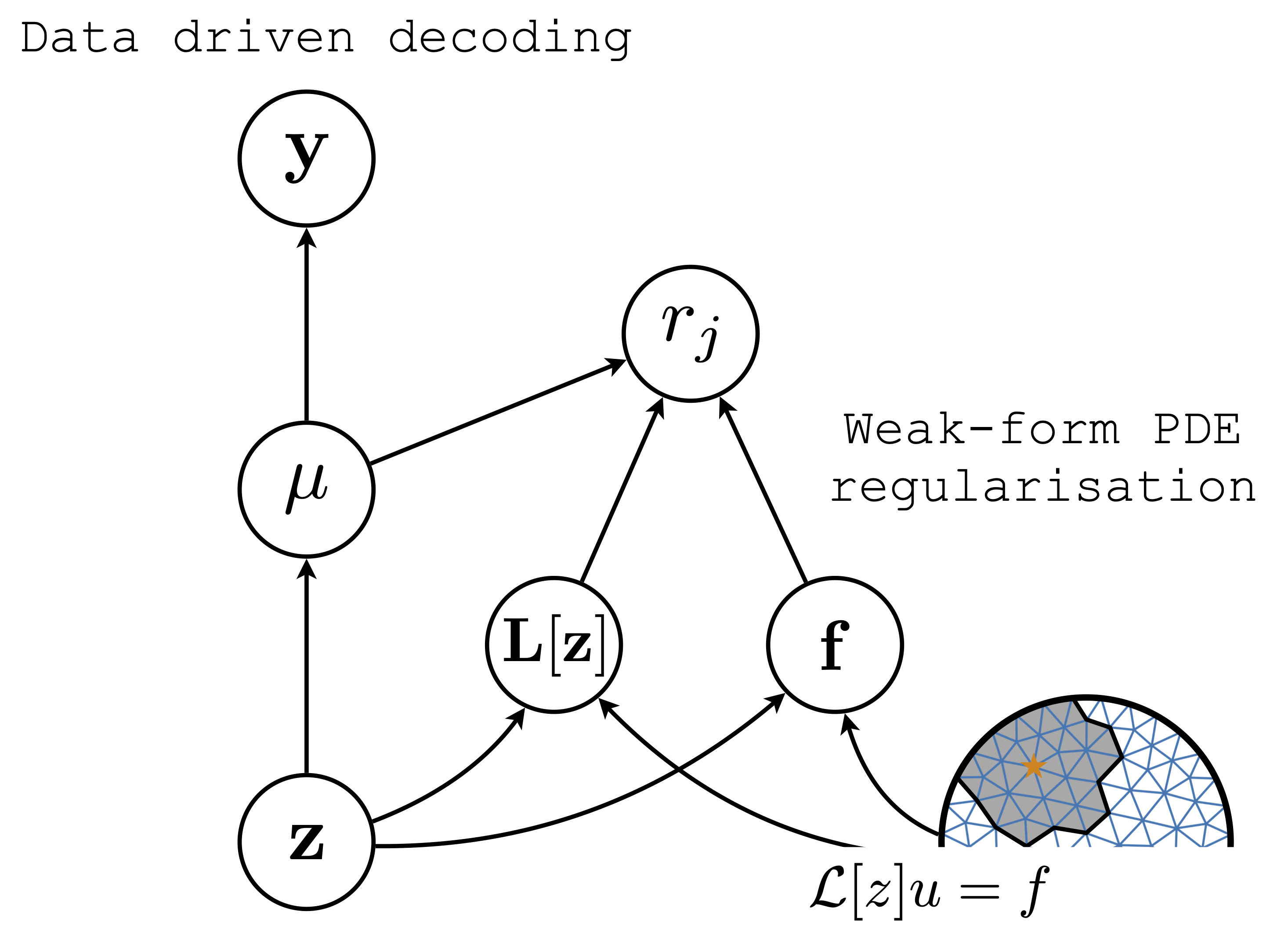
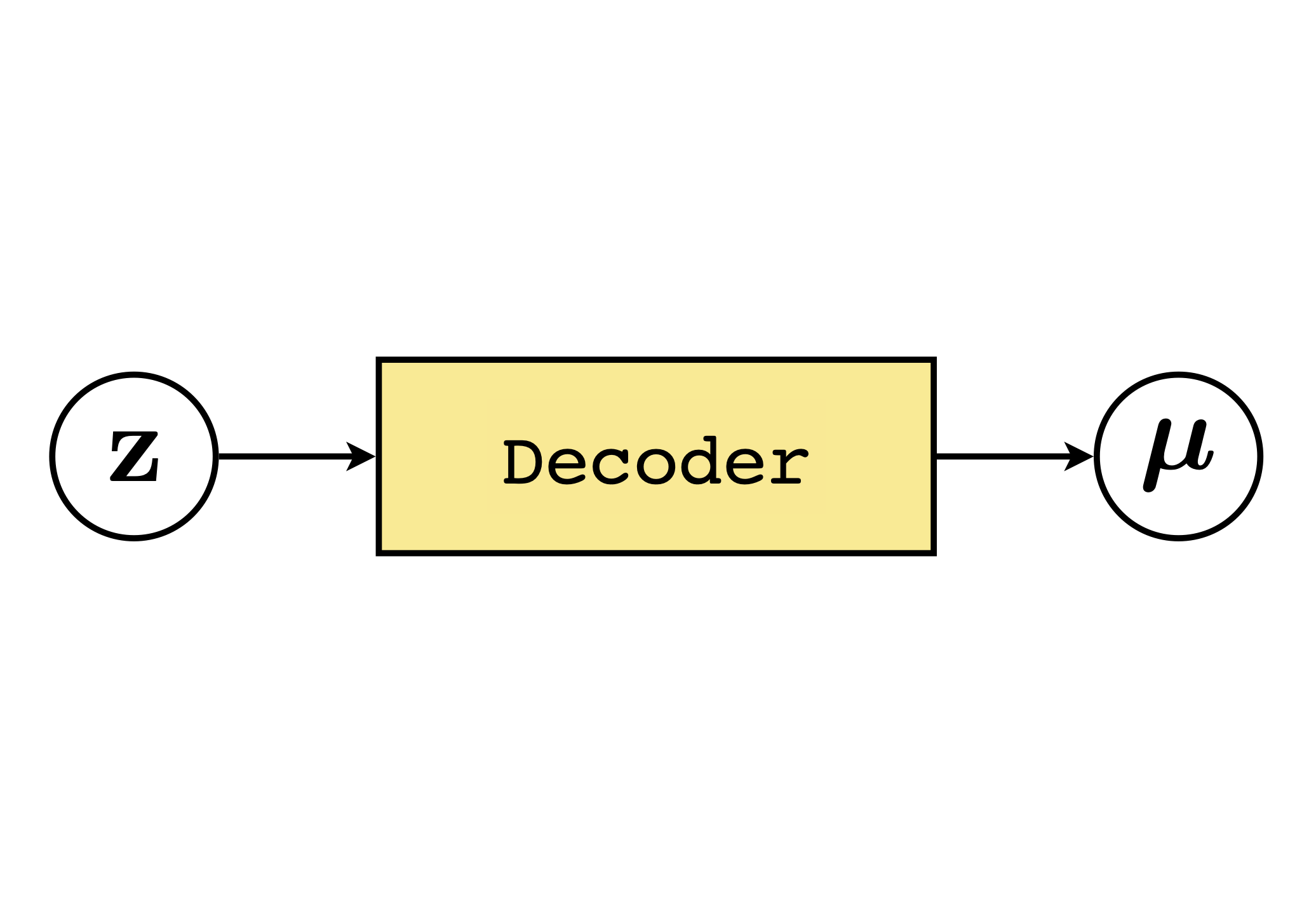
Since the sample was arbitrary we can also interpret (16b) as requiring that the random variable $r=r(\mathbf{z})$ is $\delta$-distributed. This strong constraint is the VI counterpart to the motivating problem (2). Returning to the analogy with the VAE, by removing the need to exactly solve the PDE we have allowed a high capacity free-form map to best express the data, however we reintroduce the mechanistic structure as a strong encoding term, not from the data to the latent space, but from the latent space to a point-mass determined by the mechanistic structure. This allows us to recast the augmentation of the model with a mechanistic structure, as a (pseudo)-data augmentation scheme with the new output-target pairs given by $\{(\mathbf{z}_{m},0)\}_{m=1}^{M}$, and auxillary data taking the form of a mechanistic model and its dense FEM discretisation; this resulting decoder is displayed in Fig. 2(a).

After passing to the limit in (16) the dependence on the additive perturbation, has disappeared. If one has complete confidence in the specified model this limiting problem may be desirable, however the imposition of hard constraints in ML architectures remains under-developed, [28]. Of more philosophical import; it is unlikely we would ever posses such absolute certainty. The relaxation we introduce quantifies uncertainty in the forward map, accounting for unknown physics and the over-simplifications that occur when deriving mathematical models of complex processes.

(a) PDE regularised decoder

(b) Local mini-patch approximation

Figure 2: (a) Regularisation of a standard decoder network with the weak form PDE structure. (b) Illustration of our tapering approach to construct local regularisers for computational efficiency.

4 Fast forward approximations

We have reduced the work done solving the BIP to optimising a variational distribution, $q(\mathbf{z})$, and a variational parameter, $\mu$, penalised by applying the FEM weak-form constraint (16b). It is instructive to consider approaches [39, 34] that have used the classical form (3) to construct regularisers

$$\frac{1}{N_{\text{int}}}\sum_{i=1}^{N_{\text{int}}}\left(\mathcal{L}[\mathbf{z}](\mu(\mathbf{x}_{i})-f(\mathbf{x}_{i})\right)^{2}+\frac{1}{N_{\text{bnd}}}\sum_{j=1}^{N_{\text{bnd}}}\left(\mu(\mathbf{s}_{j})-g(\mathbf{s}_{j})\right)^{2},$$ (17)

where $\{\mathbf{x}_{i}\}_{i=1}^{N_{\text{int}}}$ and $\{\mathbf{\mathbf{s}}_{j}\}_{j=1}^{N_{\text{bnd}}}$ are sampled uniformly from the interior, and boundary. This allows efficient batched gradient descent, however it is unclear how to extend this to produce a generative model. We could try and modify our approach in Sec. 3.1 by viewing (17) as MC approximation of

$$\exp\left\{-\frac{1}{2}\|\mathcal{L}[\mathbf{z}]u-f\|^{2}_{L^{2}(\Omega)}\right\},$$ (18)

however, the identity considered as a covariance operator is not Hilbert-Schmidt, since $\mathrm{Tr}(I)=\infty$. Therefore (18) is not a Gaussian measure preventing our Gaussian perturbation approach from being applied. By originating in the dual-space our work addresses this problem; however in doing so we augmented with the entire FEM structure, a significant increase in the computational burden compared to (17). To see this we consider an analogous MC approximation for our regulariser

$$\|\mathbf{L}[\mathbf{z}]\mu(\mathbf{x},\mathbf{z})-\mathbf{f}\|_{\mathbf{A}}^{2} =\sum_{i=1}^{N_{\text{nodes}}}(\mathbf{L}[\mathbf{z}]\mu(\mathbf{x},\mathbf{z})-\mathbf{f})_{i}\sum_{j\;:\;(\mathbf{A}^{-1})_{ij}\neq 0}(\mathbf{A}^{-1})_{ij}(\mathbf{L}[\mathbf{z}]\mu(\mathbf{x},\mathbf{z})-\mathbf{f})_{j}$$

$$\stackrel{{\scriptstyle\Delta}}{{=}}\sum_{i=1}^{N_{\text{nodes}}}r_{\mathbf{A}}^{(i)}(\mathbf{z})\approx\frac{1}{P}\sum_{p=1}^{P}r_{\mathbf{A}}^{(i_{p})}(\mathbf{z}),\qquad i_{1},\ldots,i_{P}\sim\mathrm{Uniform}(N_{\text{nodes}})$$ (19)

where we have replaced the full outer sum, with $P\ll N_{\text{nodes}}$ summands by uniformly sampling from the complete node set. Unfortunately, while $\mathbf{A}$ is sparse, the precision $(\mathbf{A})^{-1}$ will not be, so that each $r^{(i_{p})}_{\mathbf{A}}$ requires a complete Assembly, preventing the efficient batching possible in (17).

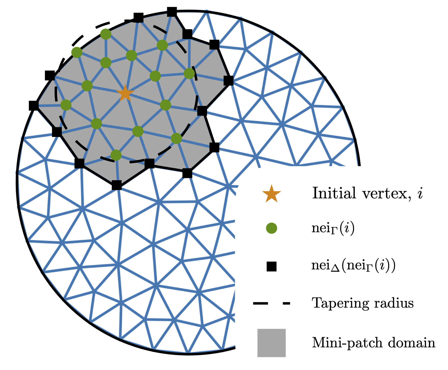
To handle this we propose replacing the precision with a suitably tapered version. This technique has been successfully applied in geostatistics [16, 15] and constructs a new matrix $\boldsymbol{\Gamma}=(\mathbf{A})^{-1}\circ\mathbf{K}_{\text{taper}}$, where $\mathbf{K}_{\text{taper}}$ is the Gram matrix of some tapering function chosen so that $(\mathbf{K}_{\text{taper}})_{ij}=0$ whenever $\|\bar{\mathbf{x}}_{i}-\bar{\mathbf{x}}_{j}\|>\rho$ for some $\rho>0$. We define the $\Gamma$-neighbourhood of a vertex $i$ to be $\text{nei}_{\Gamma}(i)=\{j\;:\;(\Gamma)_{ij}\neq 0\}$, then approximate $r^{(i)}_{\mathbf{A}}$ by $r^{(i)}_{\Gamma}$, so reintroducing sparsity into our regularisation. Evaluation of the terms $r^{(i)}_{\Gamma}$ will require the values of spatially varying processes over the set of index points $\{i\}\cup\mathrm{nei}_{\Gamma}(i)\cup\mathrm{nei}_{\Delta}(\mathrm{nei}_{\Gamma}(i))$, where $\mathrm{nei}_{\Delta}$ is the natural neighbourhood structure of a FEM mesh. This collection of nodes implicitly defines a reduced set of elements over which we need to evaluate the weak form, $\mathbb{T}^{\text{active}},$ which we refer to as a mini-patch, and display in Figure 2(b).

Assembly over this reduced mesh will be substantially cheaper than that over the full mesh, and in effect corresponds to replacing our model in Section 3.1 with a misspecified covariance function [41, 15]. Combined with sampling from the process $\mathbf{z}$ we arrive at an efficient MC approximation to the complete penalty by independently sampling $q(\mathbf{z})$, and an initial vertex $i$ around which to build the mini-patch, obtaining the hierarchical estimate

$$\mathbb{E}_{\mathbf{z}\sim q(\mathbf{z})}\left[\|\mathbf{L}[\mathbf{z}]\mu(\mathbf{x},\mathbf{z})-\mathbf{f}\|_{\mathbf{A}}^{2}\right]\approx\frac{1}{M}\sum_{n=1}^{M}\frac{1}{P}\sum_{p=1}^{P}r^{(i_{p})}_{\Gamma}(\mathbf{z}_{n}),\quad\mathbf{z}_{n}\sim q(\mathbf{z}),\quad i_{p}\stackrel{{\scriptstyle\text{i.i.d}}}{{\sim}}\mathrm{Unif}(N_{\text{nodes}})$$

By re-sampling the patch at each step of the optimisation we ensure this local constraint is applied everywhere so achieving global regularisation of the data-driven map. In the next section we empirically demonstrate the accuracy of this approximation, further study is provided in the supplement.

5 Experiments

(a) VAE

(b) VAE-DT

(c) VAE-NLD

Figure 3: PDE regularised decoder networks for the generative models in the Jura experiment. (a) presents the base VAE model, (b) and (c) augment the decoder network with a regularising PDE operator and an input source, for full details of the architechtures used see Sec. 4 of the supplement.

Our aim in this section is threefold; to demonstrate the accuracy of our method compared to ground-truth, to quantify computational efficiency and finally to demonstrate applicability to real world problems. All experiments were run on a 2.9 GHz i9 processor with 2400MHz RAM. See the supplement for discussion on the architectures and training setup used for each experiment.

Mini-patching accuracy and efficiency

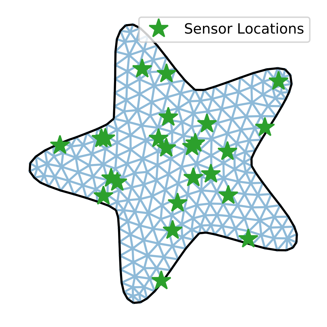
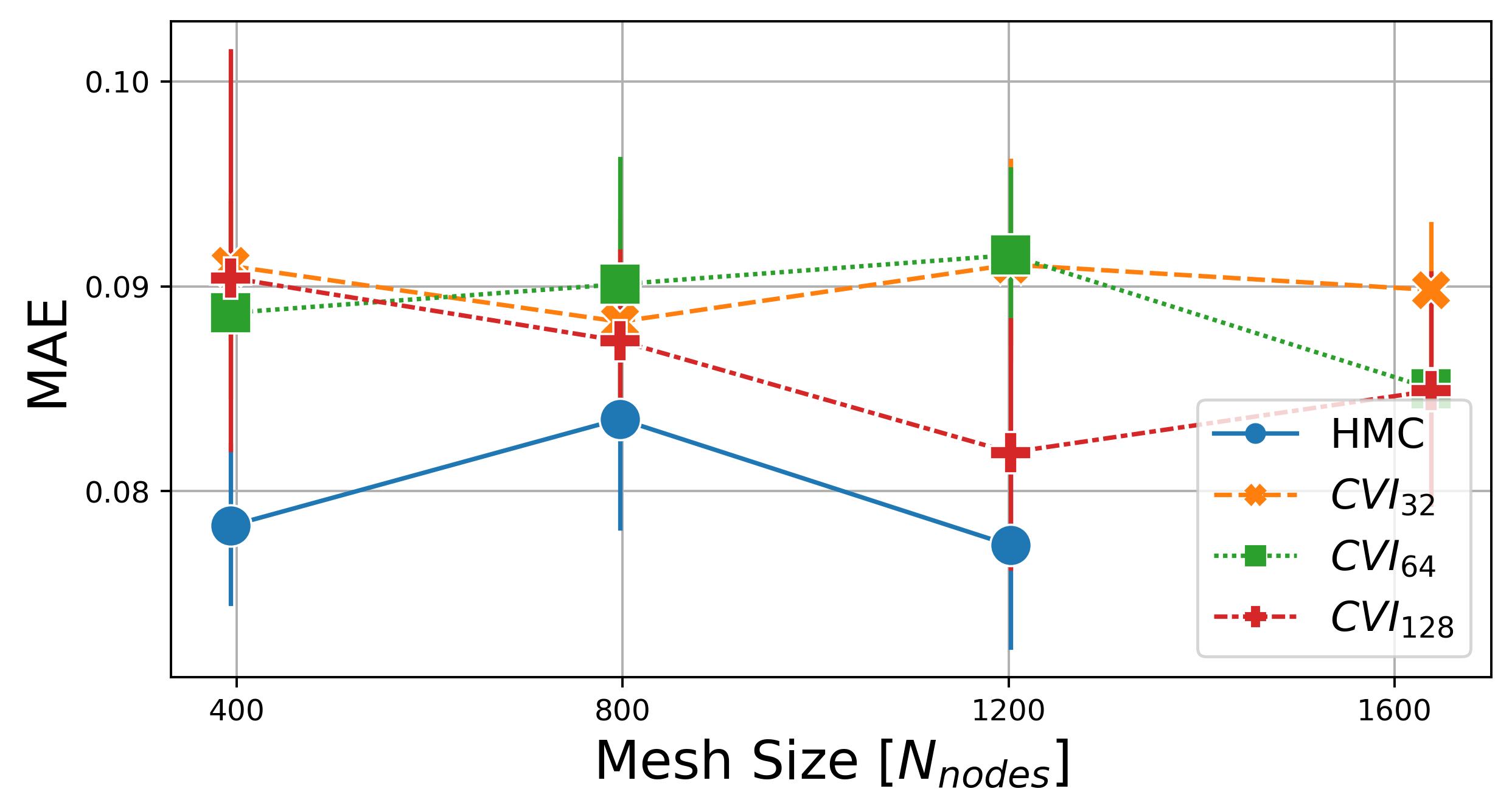
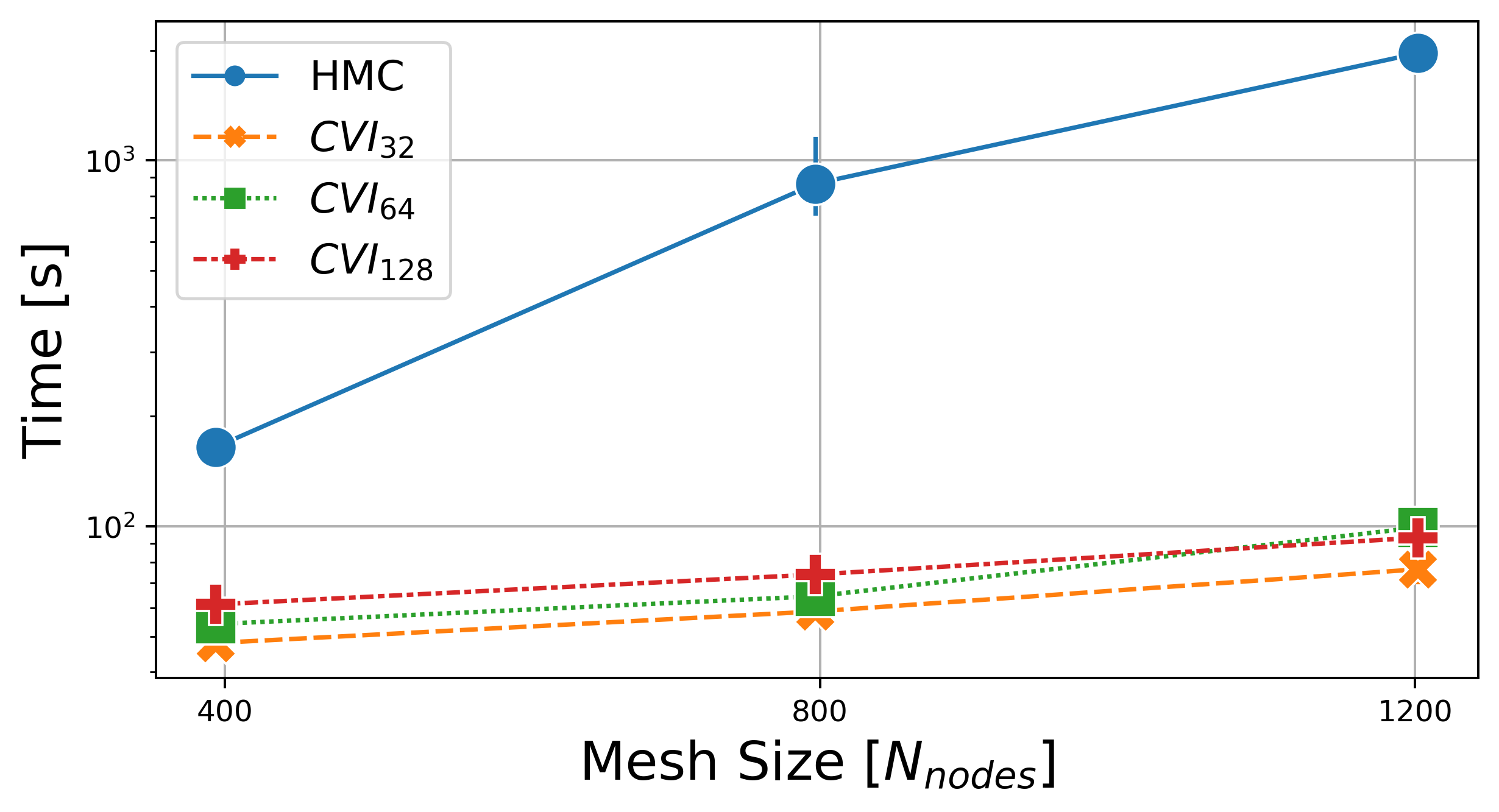
We perform the experiment depicted in Fig. 1, simulating from (4) with constant source on increasingly fine meshes. To assess our PDE constrained VI method we implement it with varying tapering chosen so that each sub-mesh had on average $Q_{\text{int}}\in\{32,64,128\}$ nodes, the specifications are labelled as $\text{CVI}_{Q_{\text{int}}}$. These are compared to the benchmark Hamiltonian Monte Carlo (HMC) [14]. We learn the posterior of the transport vector field, and compare the mean absolute error (MAE) on validation data using samples from the learned models.

Results are presented in Fig. 4(a) for all methods after a total of 10000 training iterations, as expected the HMC methods shows the best absolute performance. However, even at the smallest patch size we are able to match performance within error bounds, and at a substantially reduced cost. Fig. 4(b) reports total run-time on a log-scale where we observe the $\mathcal{O}(N_{\text{nodes}}^{3})$ scaling of the Solve in the HMC method, conversely our regulariser scales as $\mathcal{O}(N_{\text{mini-patch}}^{2})$ where $N_{\text{mini-patch}}$ is the maximum number of nodes in a mini-patch, allowing our method to be applied even on very dense meshes.

(a) Accuracy

(b) Total Run-time

Figure 4: Effect of increasing mesh resolution on accuracy and total run-time of our accelerated local approximation compared to ground truth HMC on 10 rpelicates of the transport problem. Results of HMC on the finest mesh are not shown because time taken exceeded computational budget.

Heavy metal contamination, Swiss Jura

Diffusion and transport through topsoil and waterways can lead to wide dispersal of contaminants. Since these physical influences are common to each contaminant we can use the presence of secondary metals to infer the concentration of a primary metal, here cadmium, copper, lead and cobolt, and this analysis is undertaken by [18] via kriging.

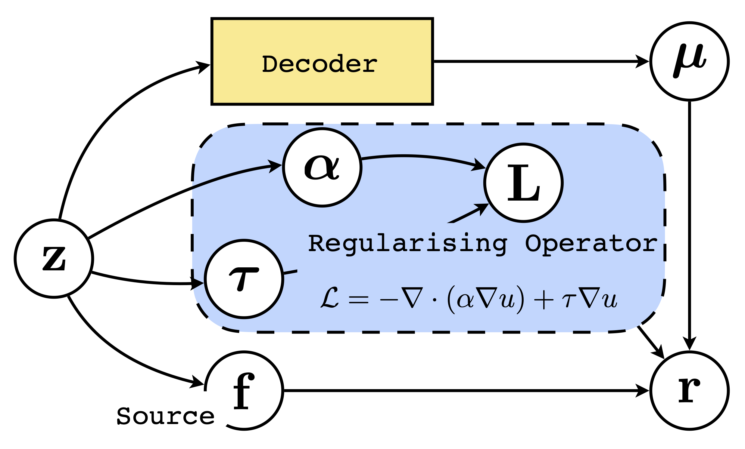
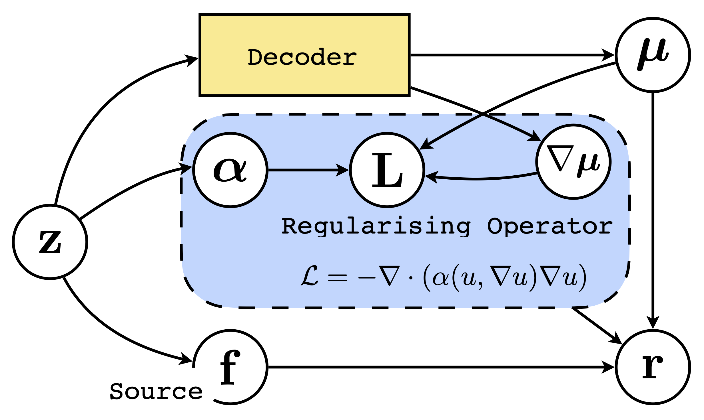
To demonstrate our method as a plug-in enhancement to a generic model we shall consider a VAE [25, 36], with generic decoder Fig. 3(a), and then add our mechanism-based regularisation. First VAE-DT, the PDE (4) with diffusion and transport which will have the generative structure in Fig. 3(b), and then VAE-NLD, a nonlinear model with diffusion operator $\mathcal{L}[\mathbf{z}]=-\nabla\cdot(a(\mathbf{z},u,\nabla u)\nabla u)$ shown in Fig. 3(c). Allowing the diffusion coefficient to be a function of the field variable and the gradient has been shown [37] to lead to stronger feature preservation. We further compare our model to the GP diffusion kernel model of [3], a linear PDE with constant diffusion and no transport. Results are displayed in Table 1; these demonstrate that the VAE was consistently outperformed, but that once our physically informed regularisation was included it was able to outperform or match accross all settings. We stress that the base architecture was constant for each VAE, indicating the ability of the method we introduce in this paper to act as a drop-in enhancement to existing architectures.

Table 1: MAE from ten repetitions of prediced heavy metal concentration on the Jura dataset. GPDK is the diffusion kernel [3]. VAE-DT and VAE-NLD extend VAE with our PDE regularisation. Results in bold indicate significance under a Wilcoxon test comparing each VAE model to the GPDK

	GPDK [3]	VAE [25, 36]	VAE-DT	VAE-NLD
Cd	$\boldsymbol{0.451\pm 0.013}$	$0.569\pm 0.115$	$0.478\pm 0.048$	$0.549\pm 0.173$
Cu	$\boldsymbol{7.168\pm 0.347}$	$7.752\pm 0.341$	$7.218\pm 0.315$	$7.625\pm 0.201$
Pb	$10.101\pm 0.284$	$15.69\pm 0.294$	$10.058\pm 0.297$	$\boldsymbol{9.722\pm 0.251}$
Co	$1.755\pm 0.090$	$1.820\pm 0.102$	$1.801\pm 0.173$	$\boldsymbol{1.692\pm 0.083}$

Eastern Snake River Plain Aquifer, Idaho

An aquifer is an underground layer of permeable rock, from which groundwater can be extracted. Geological properties govern how water permeates, and local hydrological features act as additional inputs to the system. To capture these physical processes we consider two different PDE specifications, each having a latent GP source function. The first, GP-D, possesses an inhomogenous log-GP diffusion coefficient capturing spatially varying diffusion, the second, GP-DT, is augmented with a spatially homogeneous transport field.

Figure 5: Mean predicted depth (in feet) to the groundwater level from our GP-DT

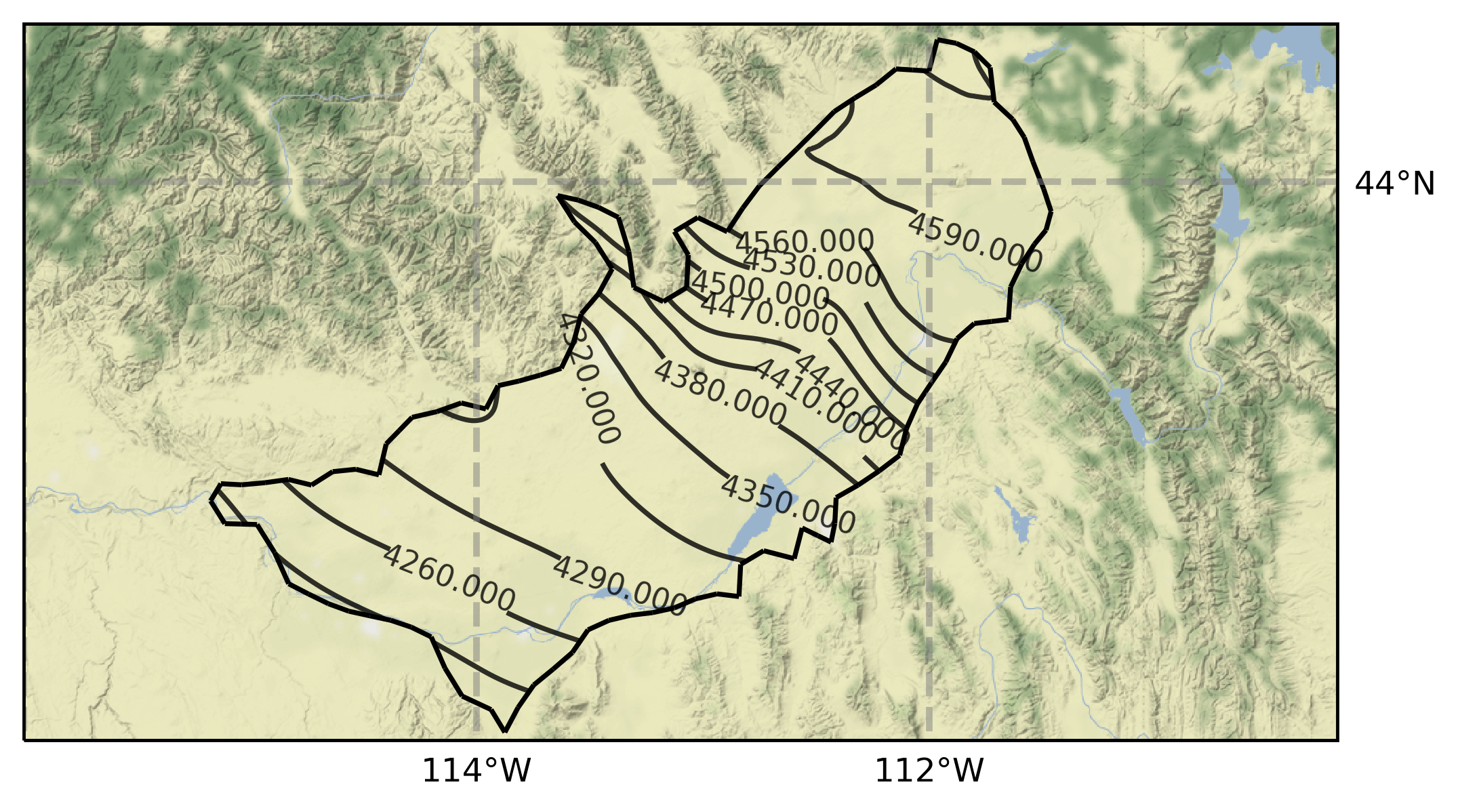
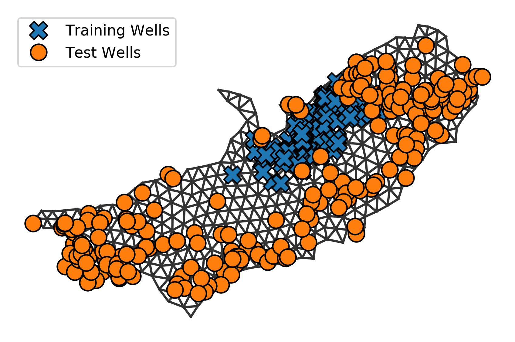
The resulting generative structure is similar to that of Fig. 3(b), see Sec. 4 of the supplement for the full presentation of the model. We train on levels from 202 wells over the period 1960–1980 reported in [2], and predict on a further set of 242 measurements from 1980–2000 .

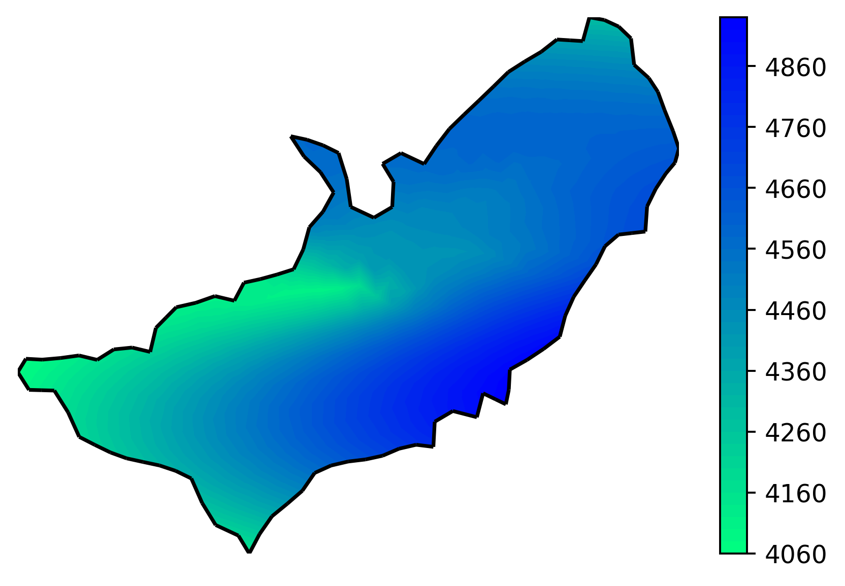
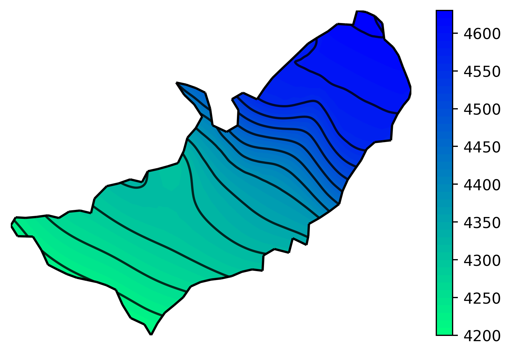
Our PDE influenced specifications are compared with baseline predictions from models encoding no physical structure; namely a GP with Matern kernel and, to allow more complex data-driven patterns, a 2-layer Deep GP (DGP) [11]. Results are displayed in Table 2 where we find that the PDE regulated models, embodying the richest physical structure outperform the mechanistically simpler alternatives. The predicted groundwater level is displayed in Fig. 5, agreeing with the output of numerical work presented in [2]. To view additional figures, including the estimated parameters, see the supplementary material.

Table 2: Validation error for the aquifer data on well measurements from 1980–2000. GP-D is our model with GP source and log-GP diffusion coefficient, GP-DT is further augmented with a transport vector field. We report mean absolute and mean squared error ($\pm 2$ standard deviations).

	GP	DGP [11]	GP-D	GP-DT
MAE	$0.224\pm 0.041$	$0.193\pm 0.052$	$0.160\pm 0.012$	$\boldsymbol{0.158\pm 0.001}$
MSE	$0.107\pm 0.050$	$0.081\pm 0.011$	$0.044\pm 0.001$	$\boldsymbol{0.039\pm 0.001}$

6 Discussion

We have considered the problem of accelerating the BIP by constructing VI approximations which respect the generative structure of the mechanistic model. By taking an optimisation-centric view beginning in the dual space we are able to soften the hard constraints of the original problem and implement a method which is able to achieve increased computational efficiency, without sacrificing accuracy. Our experiments demonstrated that our approach can be used both to accelerate the classical BIP and as a drop-in enhancement to more general methods. Beyond this we have introduced a framework which allows for the uncertainty in the governing dynamics, enabling what prior physical knowledge exists to be easily combined with flexible ML methods allowing one to leverage the full power of these methods, without ignoring the wealth of scientific knowledge already available.

Broader Impact

Our work both accelerates the classical inverse problem, and offers improved uncertainty quantification (UQ) in the presence or prior, but possibly incomplete, physical knowledge, arguably the most realistic knowledge state in real-world applications. By designing our method as a plug-in enhancement, and by virtue of the predominance of the FEM in industry [20], we ensure that our method will be more immediately familiar to engineers than model free methods. Thereby allowing for improved uptake of ML techniques in industries which have been slower to adopt statistical methods compared to newer technological sectors. Improved UQ in these industries is vital for reasons including the specification of warranties and providing failure prediction and prevention, furthermore our application to contaminants and water-level modelling is of immediate importance to public policy in drought afflicted regions, or ensuring safe drinking water in industrialised regions. Given the high potential human cost in all of the above mentioned use cases it is vital that the predictions on which warranty or policy decisions are based be transparent and accountable for. Transparency and interpretability can be particularly problematic for general DL methods, however by including a mechanistic component inside the decoder architecture we allow for a level of structure-based interpretation that would not be possible with a purely data-driven deep generative method.

Furthermore, our mini-patching idea invites future study into how local information can be better used to regularise global mechanistic models. As edge based computing continues to grow in importance integrating local information into global models will become increasingly fundamental. We have integrated well-level readings into a large scale hydrological model, but such an approach would apply equally to using phones and wearable technology as local pressure/temperature sensors as inputs into large-scale climate models. Rightly a great deal of importance is placed on the privacy of an individuals location data, and it will therefore be important that future work on this front proceeds in a way that both respects privacy, but also fully utilises the potential of local models to inform a global mechanism which our work has begun to develop.

Appendices

Appendix A Additional details of the FEM

This paper has aimed to combine several areas, most notably the solution of PDEs by the finite element method, and the use of deep probabilistic generative models in machine learning. We therefore provide some additional information regarding the FEM method, mostly concerning notational points, that was not included in the main body, however for a more comprehensive review see [35, 5].

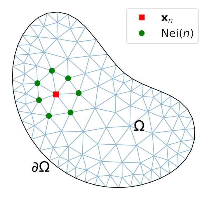
When necessary we shall denote a node in the mesh using bar notation, and the complete set of nodes by $\{\bar{\mathbf{x}}_{j}\}_{j=1}^{N_{\text{nodes}}}$. A FEM mesh naturally applies an adjacency structure to this node set with node $j\in\mathrm{nei}_{\Delta}(i)$ if there is an edge of the mesh between these two nodes, this is depicted in Fig. 6(a). We use the notation $\mathrm{nei}_{\Delta}$ to distinguish this adjacency structure arising from the mesh elements with the adjacency structure introduced in Sec. 4 from the tapering function.

The basis function used in the FEM is typically a nodal basis function, which is characterised by the fact that

$$\phi_{i}(\bar{\mathbf{x}}_{j})=\delta_{ij}$$

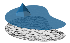
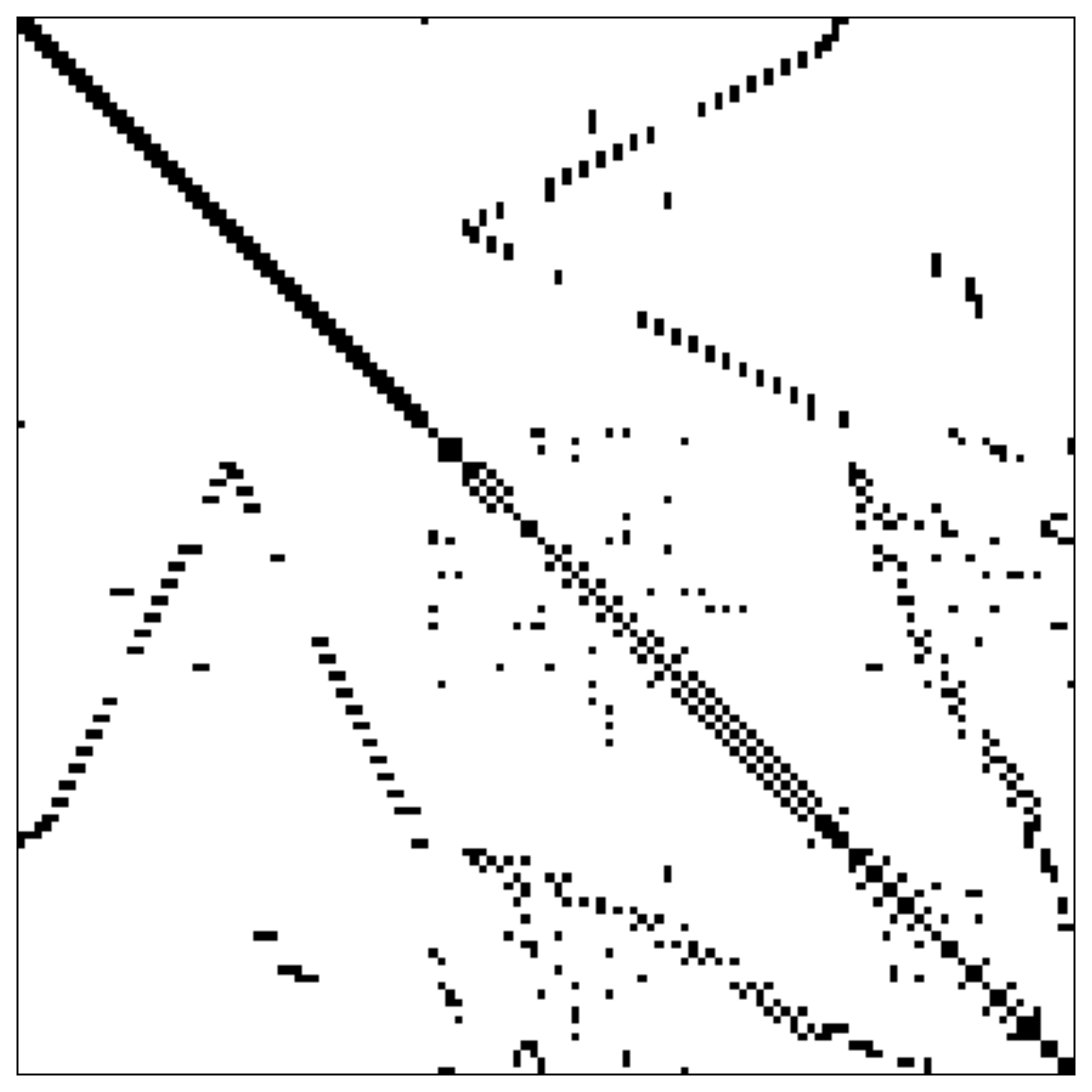
this leads to the incredible sparsity of the FEM construction. Indeed the functions $\phi_{i}$ now only have support on the set of elements with $\bar{\mathbf{x}}_{i}$ as a vertex, this is displayed in Fig. 6(b). This leads to a much smaller quadrature in the variational problem (6) and the assemblys of (7) or (8). This is seen in Fig. 6(c) where plot the sparsity patern of a typical stiffness matrix $\mathbf{A}$.

We noted in Sec. 2 that solving the PDE problem then involves solving for the coefficient $\boldsymbol{\xi}^{u}$ in equations such as

$$\mathbf{A}\boldsymbol{\xi}^{u}=\mathbf{f},$$

and this defines a function $u(\mathbf{x})=\sum_{m=1}^{M}(\boldsymbol{\xi}^{u})_{m}\phi_{m}(\mathbf{x})$ in $V$. For notational convenience we shall also refer to the vector $\boldsymbol{\xi}^{u}$ as a “function”, with the understanding that when we do so we are actually referring to the just described expansion. When doing so we shall use the more direct notation $\mathbf{u}$ for this finite dimensional representation of the function $u(\mathbf{x})$.

(a) FEM Mesh

(b) A nodal basis function

(c) Stiffness matrix sparsity

Figure 6: (a) Decomposition of a spatial domain $\Omega$ into a FEM mesh, $\Omega=\cup_{k\in\mathbb{T}}\Delta_{k}$. (b) An example nodal basis function. (c) Sparsity pattern of the stiffness matrix after assembly using nodal basis functions, upper-left block corresponds to boundary nodes which have lower connectivity.

Appendix B Additional details for Section 3

A Dual-space perturbation

In this section we provide additional details concerning our dual-space pertubation introduced in Sec. 3.1, doing so requires some familiarity with the concept of a Sobolev space, a particular instance of a reproducing kernel Hilbert space (RKHS) and its dual space, for an overview of this functional analytic material in a PDE setting we recommend [6].

While one often encounters the Laplace operator in the form presented in (5) as a differential operator in the strong sense taking a twice-differentiable function and outputting a new function, we can also consider an operator $-\Delta\;:\;H_{0}^{1}\rightarrow H^{-1}$ from the Sobolev space $H_{0}^{1}$ to its dual space $H^{-1}$. This operator, which we refer to as the (negative) Laplacian, takes a function $u\in H_{0}^{1}$ and maps it to the continous linear function $-\Delta[u]$ say, which acts on functions $v\in H_{0}^{1}$ by

$$-\Delta[u]v=\int_{\Omega}\nabla u(\mathbf{x})\cdot\nabla v(\mathbf{x})d\mathbf{x}.$$ (20)

This operator has an inverse, the inverse negative Laplacian, or more simply just the inverse Laplacian and denoted $(-\Delta)^{-1}$. The inverse Laplacian is then an operator $(-\Delta)^{-1}\;:\;H^{-1}\rightarrow H_{0}^{1},$ moreover this operator defines a Riesz-Fréchet isomorphism between the Sobolev space $H_{0}^{1}$ of functions with weak-derivative [6] and its dual-space [6, 22] and therefore

$$\|\varphi\|_{H^{-1}}=\|(-\Delta)^{-1}\varphi\|_{H^{1}_{0}},$$ (21)

where $\|\cdot\|_{H_{0}^{1}}$ is the Sobolev norm induced by the inner product

$$\langle u,v\rangle_{H^{1}_{0}}=\int_{\Omega}\nabla u(\mathbf{x})\cdot\nabla v(\mathbf{x})d\mathbf{x},$$ (22)

and applying the divergence theorem we also have the identity

$$\langle u,v\rangle_{H^{1}_{0}}=-\int_{\Omega}\Delta u(\mathbf{x})v(\mathbf{x})d\mathbf{x}\stackrel{{\scriptstyle\Delta}}{{=}}\langle-\Delta u,v\rangle_{L^{2}(\Omega)}$$ (23)

this change of sign after applying the divergence theorem now justifies the slight inconvenience of defining everything earlier in terms of the negative Laplacian operator.

Taken together the results above give us the chain of identities used in Section 3.1, in particular we first note that the weak form defines an element of the dual space, which will act on a function $v$ by

$$\varphi_{u,\mathbf{z}}\;:\;v\mapsto\int_{\Omega}\mathcal{L}u(\mathbf{x})v(\mathbf{x})d\mathbf{x}-\int_{\Omega}f(\mathbf{x})v(\mathbf{x})d\mathbf{x}$$ (24)

which we use the FEM to approximate as the element

$$\varphi_{u,\mathbf{z}}\approx\mathbf{L}[\mathbf{z}]\mathbf{u}-\mathbf{f}$$ (25)

where $\mathbf{u}$ is the finite vector of coefficients obtained after projecting the function $u(\mathbf{x})$ onto the finite dimensional subspace $V_{M}\subset H_{0}^{1}$. This is what we mean by the discretised version of the weak form (25), and the discrete form can be interpreted as giving us the image of the basis vectors $\hat{\phi}$, that is

$$\varphi_{u,\mathbf{z}}(\hat{\phi}_{j})\approx\left(\mathbf{L}[\mathbf{z}]\mathbf{u}-\mathbf{f}\right)_{j}.$$ (26)

Now to construct our approximate measure we shall start from the infinite-dimensional picture in the dual space, and then discretise at the end and so we briefly set aside the discrete version of the weak form operator just introduced. Then beginning from the Gaussian measure

$$\exp\left\{-\frac{1}{2\epsilon^{2}}\|\varphi_{u,\mathbf{z}}\|_{H^{-1}}\right\}$$ (27)

we apply the isomorphism (21) and then the definition (23) to get

$$\exp\left\{-\frac{1}{2\epsilon^{2}}\|\varphi_{u,\mathbf{z}}\|_{H^{-1}}\right\} =\exp\left\{-\frac{1}{2\epsilon^{2}}\|(-\Delta)^{-1}\varphi_{u,\mathbf{z}}\|_{H_{0}^{1}}\right\}$$

$$=\exp\left\{-\frac{1}{2\epsilon^{2}}\langle(-\Delta)(-\Delta)^{-1}\varphi_{u,\mathbf{z}},(-\Delta)^{-1}\varphi_{u,\mathbf{z}}\rangle_{L^{2}(\Omega)}\right\}$$

$$=\exp\left\{-\frac{1}{2\epsilon^{2}}\langle\varphi_{u,\mathbf{z}},(-\Delta)^{-1}\varphi_{u,\mathbf{z}}\rangle_{L^{2}(\Omega)}\right\}$$ (28)

Now we project all of the infinite-dimensional elements onto their finite dimensional representations so we replace $\varphi_{u,\mathbf{z}}$ with (25) and $(-\Delta)^{-1}$ by the inverse stiffness matrix $\mathbf{A}^{-1}$ to give the finite-dimensional Gaussian measure

$$\exp\left\{-\frac{1}{2\epsilon^{2}}(\mathbf{L}[\mathbf{z}]\mathbf{u}-\mathbf{f})^{\top}\mathbf{A}^{-1}(\mathbf{L}[\mathbf{z}]\mathbf{u}-\mathbf{f})\right\}$$ (29)

which is exactly our approximating measure for the relaxed weak form problem.

In Sec. 3 and Sec. 4 we repeatedly penalise our model by the expression

$$\|\mathbf{L}[\mathbf{z}]\mu(\mathbf{z})-\mathbf{f}\|_{\mathbf{A}},$$

the derivations above allow us to understand this intuitively as measuring the deviation of the dual-space element $\varphi_{\mu,\mathbf{z}}$ obtained using the forward-surrogate from zero, which would be the value of the element $\varphi_{G[\mathbf{z}],\mathbf{z}}$ where we recall from Sec. 2 that $G$ is the forward map, i.e. the implicit solution of the true PDE. We are then measuring the scale of these deviations under a Gaussian measure centered on zero with scale parameter $\epsilon$, and we view the measured elements $\varphi_{\mu,\mathbf{z}}$ which no longer satisfy the PDE constraint exactly as “approximate mechanisms” as remarked at the end of Sec. 3.

B The optimisation problem

In general the forward surrogate $\mu$ will depend on the spatial coordinate, however to improve presentation we suppress this dependence in the following and simply write $\mu(\mathbf{z})$ to denote the dependence of this variable on the latent processes.

Recall from Section 3 that we choose to parameterise the conditional variational factor of the forward model as the Gaussian

$$q(\mathbf{u}\mid\mathbf{z})=\mathcal{N}(\mathbf{u}\mid\mu(\mathbf{z}),\epsilon^{2}(\mathbf{L}[\mathbf{z}]\mathbf{A}^{-1}\mathbf{L}[\mathbf{z}])^{-1}),$$ (30)

also recall that our target objective function is given by

$$F_{\epsilon}=\mathbb{E}_{\mathbf{u}\sim q(\mathbf{u},\mathbf{z})}\left[-\log p(\mathbf{y}\mid\mathbf{u})\right]+\operatorname{KL}(q(\mathbf{u},\mathbf{z})\|p_{\epsilon}(\mathbf{u}\mid\mathbf{z})p(\mathbf{z})).$$ (31)

Then after applying the “chain rule for divergences” to expand $\operatorname{KL}(q(\mathbf{u},\mathbf{z})\|p_{\epsilon}(\mathbf{u}\mid\mathbf{z})p(\mathbf{z}))$ we seek to minimize the following variational lower bound

$$\mathbb{E}_{\mathbf{z}\sim q(\mathbf{z})}\left[\mathbb{E}_{\mathbf{u}\sim q(\mathbf{u}\mid\mathbf{z})}\left[-\log p(\mathbf{y}\mid\mathbf{u})\right]\right]$$

$$\qquad+\operatorname{KL}(q(\mathbf{z})\|p(\mathbf{z}))$$

$$\qquad+\mathbb{E}_{\mathbf{z}\sim q(\mathbf{z})}\left[\operatorname{KL}(q(\mathbf{u}\mid\mathbf{z})\|p_{\epsilon}(\mathbf{u}\mid\mathbf{z}))\right]$$ (32)

Focusing on the final term, and using the fact that the conditional covariance matrices in $q(\cdot\mid\mathbf{z})$ and $p_{\epsilon}(\cdot\mid\mathbf{z})$ match, we have

$$\mathbb{E}_{\mathbf{z}\sim q(\mathbf{z})}\left[\operatorname{KL}(q(\mathbf{u}\mid\mathbf{z})\|p_{\epsilon}(\mathbf{u}\mid\mathbf{z}))\right]$$

$$\qquad=\frac{1}{2\epsilon^{2}}\mathbb{E}_{\mathbf{z}\sim q(\mathbf{z})}\left[(\mu(\mathbf{z})-\mathbf{L}[\mathbf{z}]^{-1}\mathbf{f})^{\top}\mathbf{L}[\mathbf{z}]\mathbf{A}^{-1}\mathbf{L}[\mathbf{z}](\mu(\mathbf{z})-\mathbf{L}[\mathbf{z}]^{-1}\mathbf{f})^{\top}\right]$$

$$\qquad=\frac{1}{2\epsilon^{2}}\mathbb{E}_{z\sim q(\mathbf{z})}\left[\|\mathbf{L}[\mathbf{z}]\mu(\mathbf{z})-\mathbf{f}\|_{\mathbf{A}}^{2}\right].$$ (33)

From which we get the expression (13) in the main body of the text.

If we now let $\{\mathbf{z}\}_{i=1}^{M}$ be a collection of independent samples from $q(\mathbf{z})$, then

$$\frac{1}{2\epsilon^{2}}\mathbb{E}_{z\sim q(\mathbf{z})}\left[\|\mathbf{L}[\mathbf{z}]\mu(\mathbf{z})-\mathbf{f}\|_{\mathbf{A}}^{2}\right]\approx\frac{1}{M}\sum_{i=1}^{M}\|\mathbf{L}[\mathbf{z}_{i}]\mu(\mathbf{z}_{i})-\mathbf{f}\|_{\mathbf{A}}^{2}$$ (34)

The full approximate objective function after applying a Monte-Carlo approximation to the objective function is therefore given by

$$F_{\epsilon}\approx\mathbb{E}_{\mathbf{u}\sim q(\mathbf{u},\mathbf{z})}\left[-\log p(\mathbf{y}\mid\mathbf{u})\right]+\operatorname{KL}(q(\mathbf{z})\|p(\mathbf{z}))+\frac{1}{2\epsilon^{2}M}\sum_{i=1}^{M}\|\mathbf{L}[\mathbf{z}_{i}]\mu(\mathbf{z}_{i})-\mathbf{f}\|_{\mathbf{A}}^{2}.$$ (35)

Defining the variable $\mathbf{r}_{i}\stackrel{{\scriptstyle\Delta}}{{=}}\mathbf{L}[\mathbf{z}_{i}]\mu(\mathbf{z}_{i})-\mathbf{f}$, then we recognise (35) as the quadratic penalty form of the following objective function

$$\operatorname*{arg\,min}_{q(\mathbf{z})\in\mathcal{Q},\mu\in V}\mathbb{E}_{\mathbf{u}\sim q(\mathbf{u},\mathbf{z})}\left[-\log p(\mathbf{y}\mid\mathbf{u})\right]+\operatorname{KL}(q(\mathbf{z})\|p(\mathbf{z}))$$ (36a)

$$\mbox{subject to}\quad\|\mathbf{r}_{i}\|_{\mathbf{A}}=0,\qquad i=1,\ldots,M,$$ (36b)

with $M$ constraints. Alternatively, and because the sample was arbitrary, we conclude that

$$\operatorname*{arg\,min}_{q(\mathbf{z})\in\mathcal{Q},\mu\in V}\mathbb{E}_{\mathbf{u}\sim q(\mathbf{u},\mathbf{z})}\left[-\log p(\mathbf{y}\mid\mathbf{u})\right]+\operatorname{KL}(q(\mathbf{z})\|p(\mathbf{z}))$$ (37a)

$$\mbox{subject to}\quad q(\|\mathbf{r}\|)=\delta(\|\mathbf{r}\|),$$ (37b)

Or equivalently

$$\operatorname*{arg\,min}_{q(\mathbf{z})\in\mathcal{Q},\mu\in V}\mathbb{E}_{\mathbf{u}\sim q(\mathbf{u},\mathbf{z})}\left[-\log p(\mathbf{y}\mid\mathbf{u})\right]+\operatorname{KL}(q(\mathbf{z})\|p(\mathbf{z}))$$ (38a)

$$\mbox{subject to }r(\mathbf{z}_{i})=0,\text{ for all finite samples $\{\mathbf{z}\}_{i=1}^{M}$ from $q(\mathbf{z})$}$$ (38b)

with $r(\mathbf{z})$ the scalar function defined by $r(\mathbf{z})=\left\|\mathbf{L}[\mathbf{z}]\mu(\mathbf{z})-\mathbf{f}\right\|_{\mathbf{A}}$.

C Interpretation as a VAE

In this section we provide some further details on how our our model is to be interpreted as a variational auto-encoder [25, 36] with the deocder network modulated by a supervising PDE problem, in particular we provide details on two of the simpler aspects not explored in the main paper, namely the role of the encoder network, and also how the optimisation framework in Sec. 3 modifies the usual presentation of the VAE.

First we recall that the typical variational problem for a variational auto encoder has an objective function of the form

$$-\mathbb{E}_{\mathbf{z}\sim q(\mathbf{z})}\left[\log p(\mathbf{y}\mid\mathbf{z})\right]+\operatorname{KL}(q(\mathbf{z}\mid\mathbf{y})\|p(\mathbf{z}))$$

where $p(\mathbf{y}\mid\mathbf{z})$ is some high-capacity model for the conditional probability, typically this will be parameterised by a neural-network model. We also notice at this point that our work has had relatively little to say about the encoder network $q(\mathbf{z}\mid\mathbf{y})$, this is an instance of our desire to allow as much as possible our approach to be used as a plug-in enhancement to any existing encoder/decoder architecture, and indeed any of the approaches used in the many body can be extended to this more general framework by substituting instances of $q(\mathbf{z})$ for $q(\mathbf{z}\mid\mathbf{y})$. While we have not examined this particular aspect of the model, it may still be an interesting area for future study.

Returning to the specification of the encoder likelihood function we shall consider the following model for the likelihood of sensor observations $y_{n}$ at a spatial coordinate $\mathbf{x}_{n}$

$$p(y_{n}\mid u(\mathbf{x}_{n}),\mathbf{z})=\mathcal{N}(y_{n}\mid u(\mathbf{x}_{n}),\sigma^{2}(\mathbf{z}))$$

that is we centre the observation distribution on the solution of the PDE model, but allow for heteroscedastic variance parameterised by the latent variable $\mathbf{z}$.

Then we can write

$$\mathbb{E}_{\mathbf{u}\sim q_{\epsilon}(\mathbf{u}\mid\mathbf{z})}\left[\log\mathcal{N}(y_{n}\mid u(\mathbf{x}_{n}),\sigma^{2}(\mathbf{z}))\right]$$

$$\qquad=\mathbb{E}_{\mathbf{u}\sim q_{\epsilon}(\mathbf{u}\mid\mathbf{z})}\left[-\frac{1}{2\sigma^{2}(\mathbf{z})}(y_{n}-u(\mathbf{x}_{n}))^{2}-\frac{1}{2}\log 2\pi\sigma^{2}(\mathbf{z})\right]$$

$$\qquad=-\frac{1}{2\sigma^{2}(\mathbf{z})}(y_{n}-\mu(\mathbf{z}))^{2}-\frac{1}{2}\log 2\pi\sigma^{2}(\mathbf{z})-\frac{\mathrm{Var}_{q_{\epsilon}}(\mathbf{u})}{2\sigma^{2}(\mathbf{z})}$$

$$\qquad=\log\mathcal{N}(y_{n}\mid\mu(\mathbf{z}),\sigma^{2}(\mathbf{z}))+\mathcal{O}(\epsilon^{2}).$$ (39)

where we have used the fact that the variance term of $q_{\epsilon}$ in (12) is scaled by $\epsilon^{2}$.

We can now use this to rewrite (35) as

$$\mathbb{E}_{\mathbf{z}\sim q(\mathbf{z})}\left[-\log\mathcal{N}(\mathbf{y}\mid\mu(\mathbf{z}),\sigma^{2}(\mathbf{z}))\right]+\operatorname{KL}(q(\mathbf{z})\|p(\mathbf{z}))$$

$$\qquad+\frac{1}{2\epsilon^{2}M}\sum_{i=1}^{M}\|\mathbf{L}[\mathbf{z}_{i}]\mu(\mathbf{z}_{i})-\mathbf{f}\|_{\mathbf{A}}^{2}+\mathcal{O}(\epsilon^{2})$$ (40)

after taking the limit $\epsilon\rightarrow 0$ the final term will disappear. If we also parameterise $q(\mathbf{z})$ as $q(\mathbf{z}\mid\mathbf{y})$ then we arrive at the optimisation problem

$$\operatorname*{arg\,min}_{q(\mathbf{z}\mid\mathbf{y})\in\mathcal{Q},\mu\in V}\mathbb{E}_{\mathbf{z}\sim q(\mathbf{z}\mid\mathbf{y})}\left[-\log\mathcal{N}(\mathbf{y}\mid\mu(\mathbf{z}),\sigma^{2}(\mathbf{z}))\right]+\operatorname{KL}(q(\mathbf{z}\mid\mathbf{y})\|p(\mathbf{z}))$$ (41a)

$$\mbox{subject to }r(\mathbf{z}_{i})=0,\text{ for all finite samples $\{\mathbf{z}\}_{i=1}^{M}$ from $q(\mathbf{z}\mid\mathbf{y})$}$$ (41b)

So that (41a) now takes the form of a mechanistically constrained VAE problem, this is only slightly more complex than the form (16) used in the main body of the paper and justifies our omission of a fuller discussion of the likelihood model in the main body of the work. Importantly the variance term $\sigma^{2}(\mathbf{z})$ is detached from the mean function $\mu(\mathbf{z})$, and it is only the function $\mu(\mathbf{z})$ that enters the constraint term through the constraint term $r(\mathbf{z}_{i})$ which is a function of the elements $\{\mu(\mathbf{z}_{i}),\mathbf{L}[\mathbf{z}_{i}])\}$.

Appendix C Mini-patching

Figure 7: The mini-patch formed by including all elements with a vertex which is in $\mathrm{nei}_{\Delta}(i)$, for some initial vertex. This is the reduced mesh over which we evaluate the weak-form whenever calculating the component $(\mathbf{L}[\mathbf{z}]\mu(\mathbf{z}))_{i}$ of the discretised weak-form.

In this section we provide some additional details on how our mini-patching approximation may be used to accelerate the training of the mechanistically regulated decoder. First we recall from Section 4 that the regularisation term we are seeking to approximate is given by

$$\mathcal{R}(\mathbf{z})=\|\mathbf{L}[\mathbf{z}]\mu(\mathbf{z})-\mathbf{f}\|_{\mathbf{A}}^{2}$$ (42)

We also recall that the sparsity of the nodal basis functions translates into sparsity of the operator $\mathbf{L}[\mathbf{z}]$, that is we have

$$(\mathbf{L}[\mathbf{z}]\mu(\mathbf{z}))_{i} =\sum_{j=1}^{N_{\text{nodes}}}(\mathbf{L}[\mathbf{z}])_{ij}\mu_{j}(\mathbf{z})$$

$$=\sum_{j\in\mathrm{nei}_{\Delta}(i)}(\mathbf{L}[\mathbf{z}])_{ij}\mu_{j}(\mathbf{z}).$$ (43)

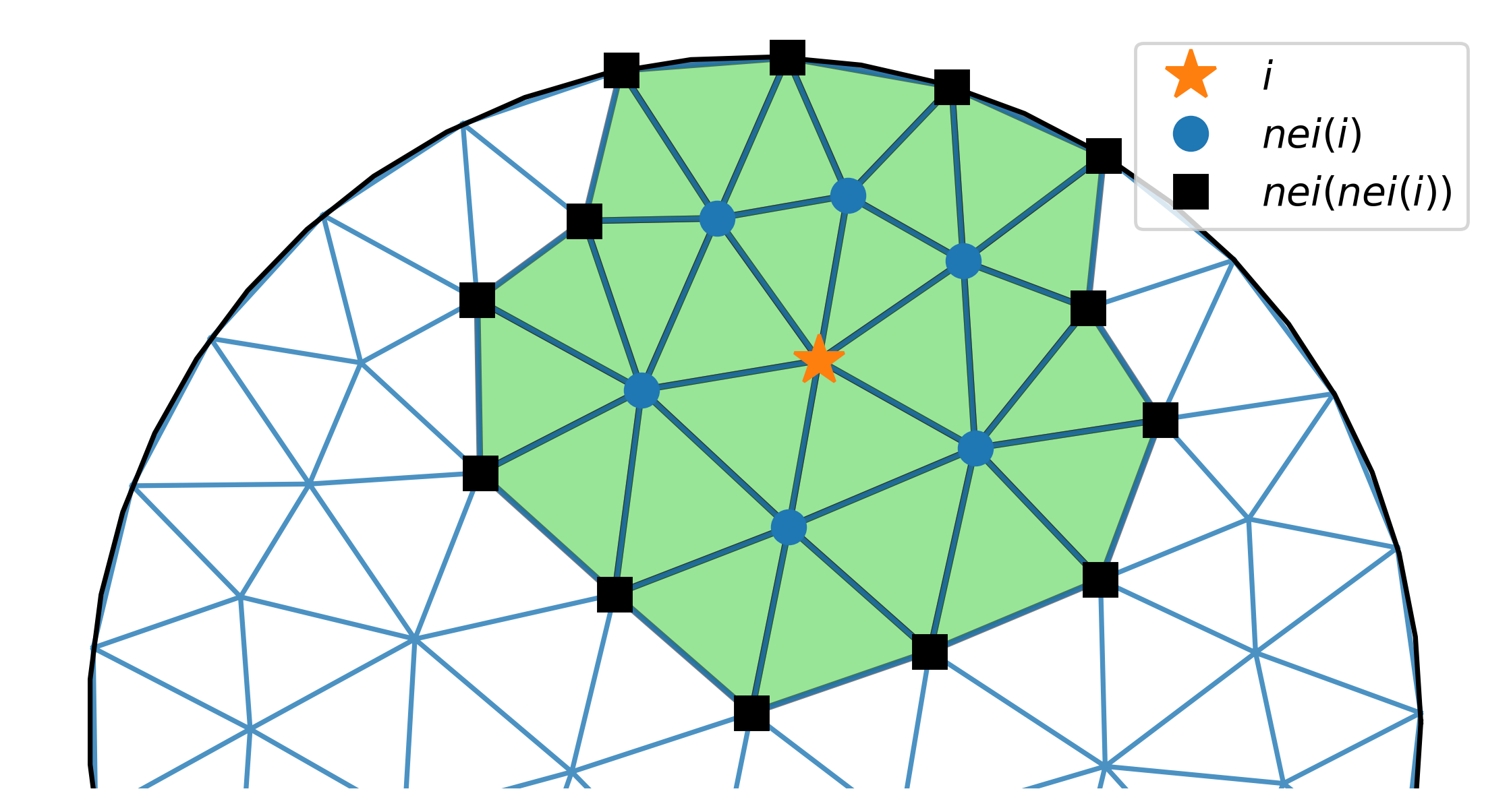
Noteably to evaluate this term we require only the values of $(\mathbf{L)}_{ij}$ on the direct neighbours of $i$, in turn this requires performing the quadrature over all mesh elements that have an element of $\mathrm{nei}_{\Delta}(i)$ as a vertex, this relationship is displayed in Fig. 7. Unfortunately, and as mentioned in the main paper, this does not translate into a useful sparsity pattern for the regulariser. Indeed we want to evaluate the value $\mathbf{r}_{\mathbf{A}}^{(i)}$ where

$$r^{(i)}_{\mathbf{A}}=(\mathbf{L}[\mathbf{z}]\mu(\mathbf{x},\mathbf{z})-\mathbf{f})_{i}\sum_{j:(\mathbf{A}^{-1})_{ij}\neq 0}(\mathbf{A}^{-1})_{ij}(\mathbf{L}[\mathbf{z}]\mu(\mathbf{x},\mathbf{z})-\mathbf{f})_{j}$$ (44)

but in general $(\mathbf{A}^{-1})$ is a dense matrix, that is

$$\{j\;:\;(\mathbf{A}^{-1})_{ij}\neq 0\}=\{j\;:\;j=1,\ldots,N_{\text{nodes}}\}$$ (45)

and is therefore of no computational benefit. However, we nevertheless should expect that the elements of the covariance matrix $\mathbf{A}^{-1}$ should decrease to zero as the distance between points increases. Based on this idea we propose to use the idea of covariance tapering to replace the covariance matrix with a localised version, $\Gamma_{\rho}$. Infact we chose to make this a hard threshold tapering and so define a tapering radius $\rho>0$ and define our new covariance term by

$$(\Gamma_{\rho})_{ij}=\begin{cases}(\mathbf{A}^{-1})_{ij}&\text{if }|\bar{\mathbf{x}}_{i}-\bar{\mathbf{x}}_{j}|<\rho\\ 0&\text{otherwise}.\end{cases}$$ (46)

The method now proceeds by choosing a vertex $i_{p}$ uniformly, assembling the matrix $\mathbf{L}[\mathbf{z}]$ only on those values in the implied mini-patch and then evaluating $r^{(i)}_{\Gamma_{\rho}}$. In principle $\Gamma$ is still an $N_{\text{nodes}}\times N_{\text{nodes}}$ matrix, however also note that because evaluating $r^{(i_{p})}$ only requires the non-zero elements in a row $(\Gamma)_{i_{p},:}$ and this is only those elements which are less that $\rho$ units from the sampled vertex $i_{p}$ we can drastically reduce the computational time by choosing $\rho$ small. This cost is also a fixed cost that can be done offline before training and then using a look-up table to index the vertex $i_{p}$ and its sparse rows. The reduction in time taken to implement our PDE regularisation method using this tapering has already been demonstrated and discussed in the transport experiment in Sec.5, it remains to demonstrate that this is still an accurate approximation to the original error, and we now consider this aspect.

A Tapering error estimates

In Section 5, and in particular in Fig. 4(a) we have already demonstrated that our mini-patching approximation leads to substantially reduced computation time on the BIP relative to the benchmark HMC method, and does so while maintaining accuracy. In this experiment we complement this by showing that the approximation introduced in Sec. 4, which allowed us to achieve the computational benefits, introduces negligible loss of accuracy compared to the true error $\mathcal{R}(\mathbf{z})$. To carry out the experiment we use the transport equation (4) with constant unit diffusion, spatially homogeneous transport vector $\boldsymbol{\tau}(\mathbf{x})=(1,1)^{\top}$ and source $f(\mathbf{x})=1$. We then perturb the model my simulating from the Gaussian perturbation we introduced in Section 3.1, with scale $\epsilon\in\{0.1,0.01\}$, that is we generate samples from the distribution

$$\mathbf{w}\sim\mathcal{N}(\mathbf{w}\mid\mathbf{0},\epsilon^{2}\mathbf{A}),$$

and form the process $w(\mathbf{x})=\sum_{i=1}^{N_{\text{nodes}}}(\mathbf{w})_{i}\phi_{i}(\mathbf{x})$. The perturbed solution is then given by solving

$$-\Delta u_{\epsilon}(\mathbf{x})+\int_{\Omega}(1,1)^{\top}\cdot\nabla u_{\epsilon}(\mathbf{x})=1+w(\mathbf{x}),$$ (47)

and we denote the coefficients parameterising the solution of this perturbation by $\mathbf{u}_{\epsilon}$. At the same time we shall assemble the discretised weak-form corresponding to the unperturbed problem, that is we assemble the matrix $\mathbf{L}$ and the vector $\mathbf{b}$ with elements

$$(\mathbf{L})_{ij}=\int_{\Omega}\nabla\phi_{j}(\mathbf{x})\nabla\phi_{i}(\mathbf{x})dx+\int_{\Omega}(1,1)^{\top}\cdot\nabla\phi_{j}(\mathbf{x})\phi_{i}(\mathbf{x})dx,\qquad(\mathbf{b}_{i})=\int_{\Omega}\varphi_{i}(x)dx,$$ (48)

and then evaluate the error terms

$$\mathbf{r}_{\epsilon,\mathbf{A}}=\|\mathbf{L}\mathbf{u}_{\epsilon}-\mathbf{b}\|_{\mathbf{A}},\qquad\mathbf{r}_{\epsilon,\Gamma_{\rho}}=\frac{1}{P}\sum_{p=1}^{P}\|\mathbf{L}\mathbf{u}_{\epsilon}-\mathbf{b}\|_{(\Gamma_{\rho})_{{i_{p}},:}},$$ (49)

where we use the notation $\|\mathbf{w}\|_{(\Gamma_{\rho})_{{i_{p}},:}}$ to denote the product of the two scalars

$$(\mathbf{w})_{i_{p}}\cdot\langle(\Gamma_{\rho})_{{i_{p}},:},\mathbf{w}\rangle_{\mathbb{R}^{N_{\text{nodes}}}}.$$

The first term in (49) is our target error, and the second of these is our tapered mini-patch approximation to this error. By perturbing we make sure this first term is not trivially equal to zero, and so investigate the behaviour of our approximation around the target value. In this experiment we report the absolute difference of these two estimates, that is we report the absolute error $|\mathbf{r}_{\epsilon,\mathbf{A}}-\mathbf{r}_{\epsilon,\Gamma_{\rho}}|$ obtained from a total of $10$ different samples of the perturbation process $w(\mathbf{x})$.

(a) Approximation error, $\epsilon=0.1$

(b) Approximation error, $\epsilon=0.01$

(c) Average mesh coverage

Figure 8: Absolute error of the tapered mini-patching approximation as a function of the tapering radius, and the number of meshes sampled, $P\in\{1,10,50\}$

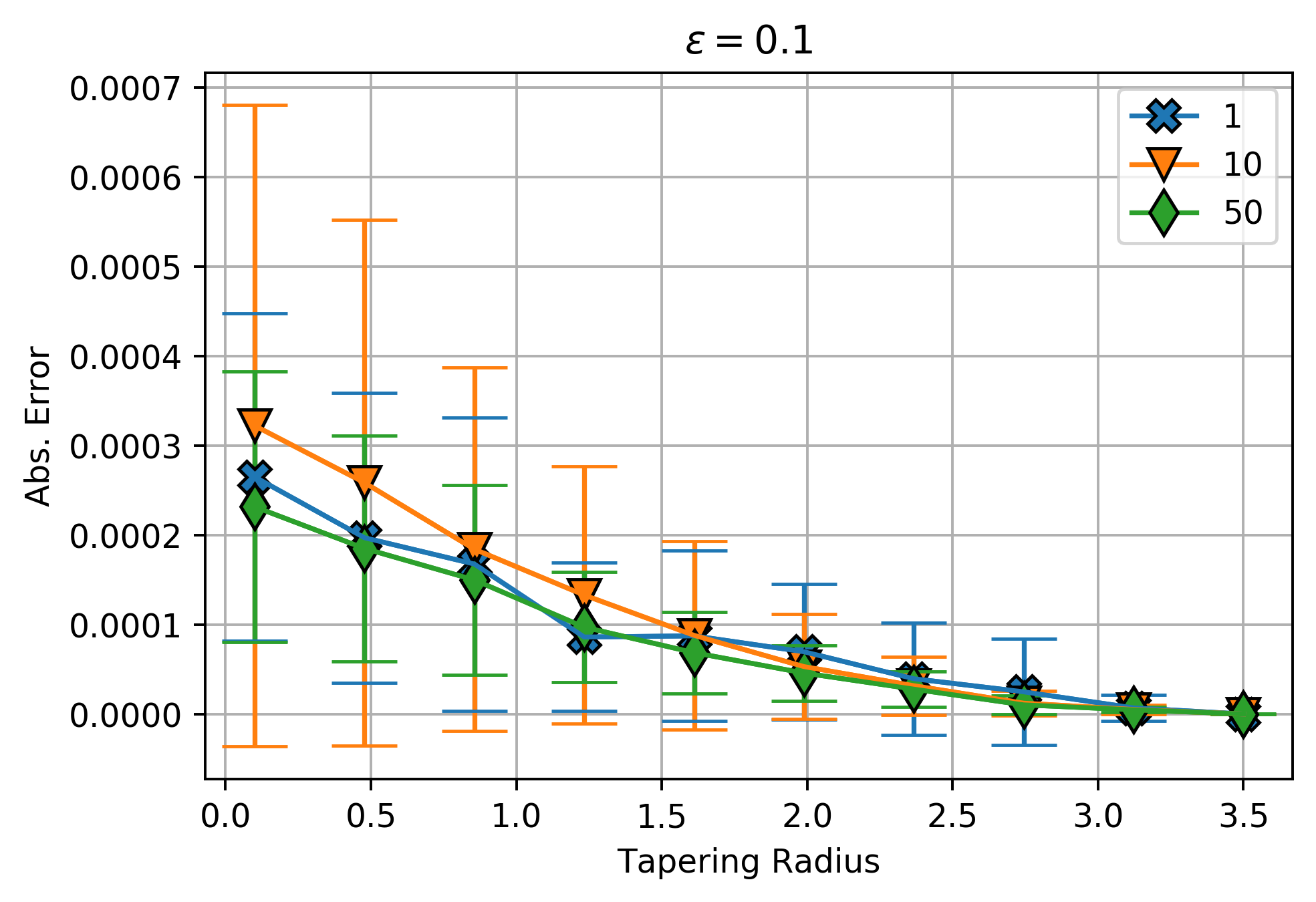
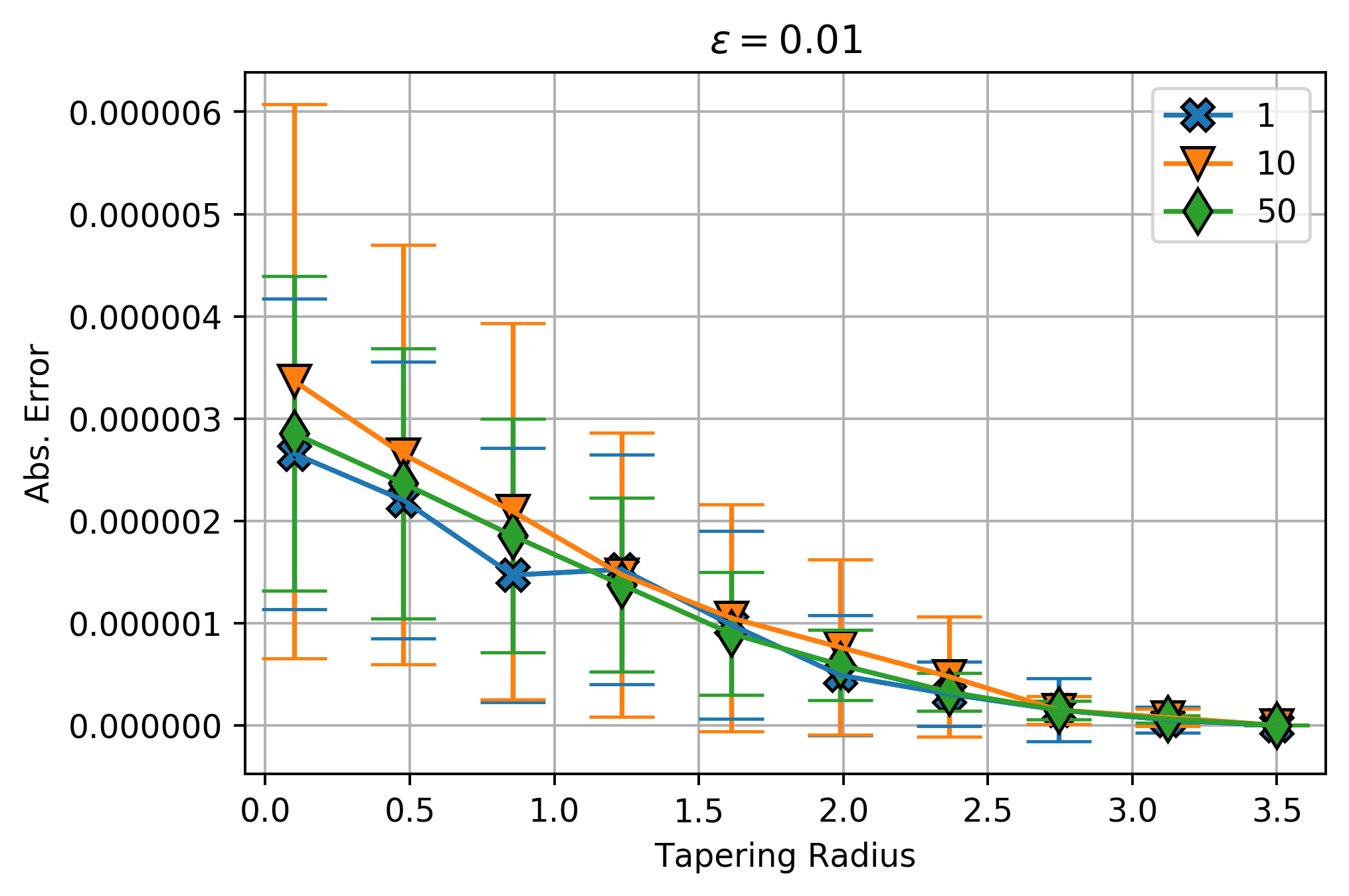
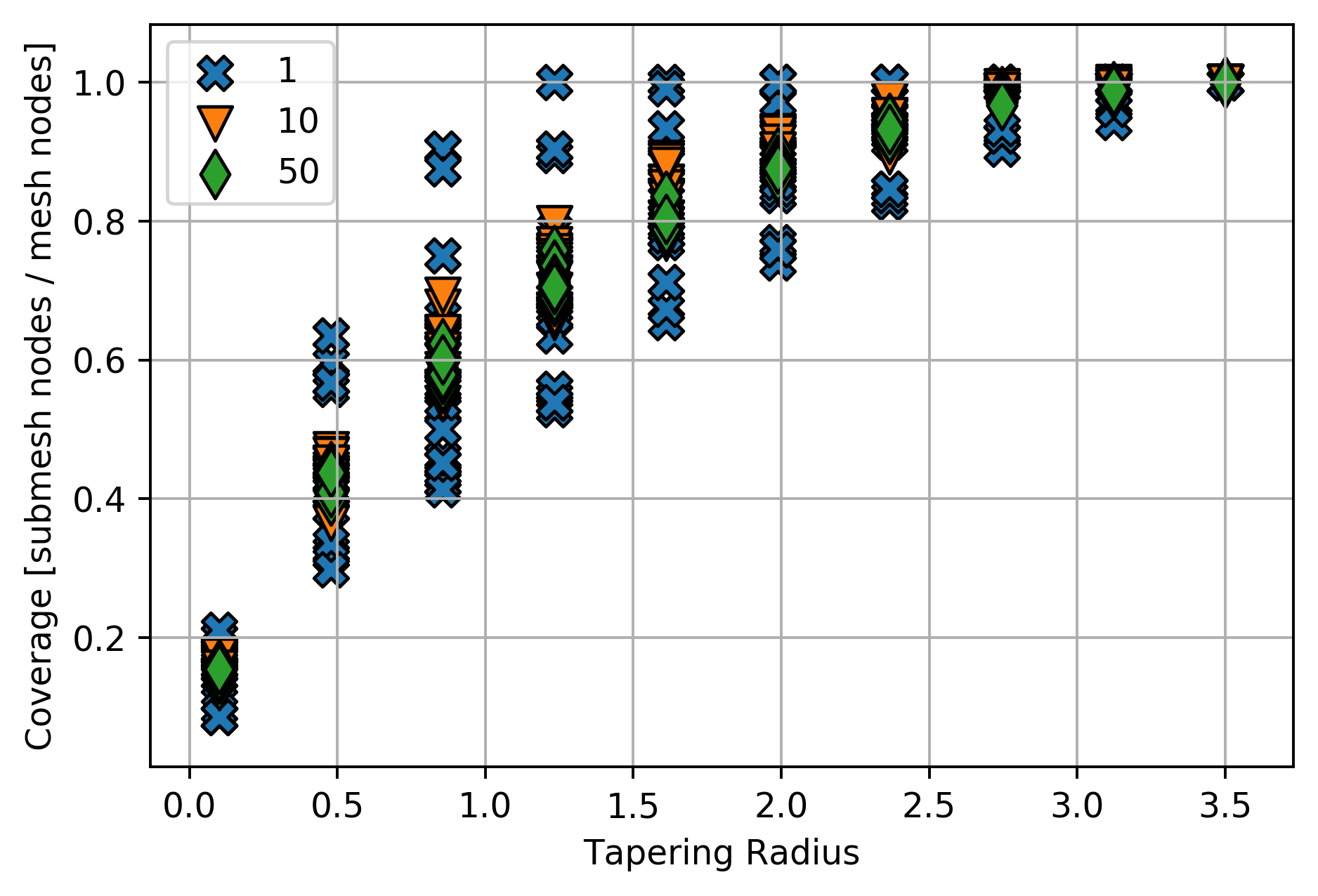
The results are displayed in Fig. 8, where we can observe that as one would expect the absolute error of the tapered approximation decreases to zero as the tapering radius increases since the tapered mesh converges to the full mesh. Importantly for the application of our method we note two important details; (i) the absolute error is small even for the smallest sub-meshes, and indeed is orders or magnitude lower than the perturbation error $\epsilon$, and (ii) that even the single sample estimate is within the error limit of the methods using more samples. Given this second remark we choose to use a single mesh sample in all of the remaining experiments reported in this paper. In Fig. 8(c) we also plot the tapering radius versus the average fraction of the whole mesh covered by a mini-patch, demonstrating that the chosen radius ranges plotted in Fig. 8 were sufficient to cover the full spectrum of relevant mesh portions.

Appendix D Further details of the experiments

In this section we provide some additional details for the experiments reported in Sec. 5 of the main paper, including the specific architecture used in each instance. All models were implemented in Tensorflow [1] including a Tensorflow implementation of the FEM, full code for which is available from the authors’ website. Optimisation was done using the Adam optimiser with default parameters.

A Jura experiment

Model specification

The form of the PDE mechanisms used to supervise the experiments was given in Fig. 3(a) but for convenience we restate them here

$$\mathcal{L}u=-\nabla\cdot(a(\mathbf{x})\nabla u)+\boldsymbol{\tau}^{\top}\cdot\nabla u$$ (50)

(a) Mechanistic form of VAE-DT

$$\mathcal{L}u=-\nabla\cdot(a(\mathbf{x},u,\nabla u)\nabla u)$$ (51)

(b) Mechanistic form of VAE-NLD

Figure 9: Mechanistic operators used to regularise the base VAE model in the Jura experiment.

Inference

As emphasised in the main paper our method is intended to augment a standard model, therefore all of the VAE variants used the same encoder/decoder network which take the forms given in Fig. 10 the models are then trained by adding our pde regularised loss to the standard variational loss as described in Sec. 3.1 of the paper.

Our objective is to use the presence of the secondary metals, to predict the concentration of a primary, that is we are attempting to learn a variational approximation to the conditional distribution $p(y^{(p)}(\mathbf{x})\mid\mathbf{x},\mathbf{s}^{(p)}(\mathbf{x}))$ where $p$ is a primary metal in $\{\text{CD},\text{CU},\text{PB},\text{CO}\}$, and $\mathbf{s}^{(p)}(\mathbf{x})$ is the value of a collection of secondary metals at that same spatial coordinate, a table of the primary and second metals from [3] is given in 3.

Table 3: Primary and secondary metals for the Jura experiment [18, 3]

Primary	Secondary
Cd	Pb, Ni, Zn
Cu	Ni, Zn
Pb	Cu, Ni, Zn
Co	Ni, Co

The conditional distribution $p(y^{(p)}(\mathbf{x})\mid\mathbf{x},\mathbf{s}^{(p)}(\mathbf{x}))$ is therefore the target of our decoder $q(\mathbf{y}\mid\mathbf{z},\mathbf{x},\mathbf{s})$, and we learn this factor for a base VAE model, and the PDE regularising operators in Fig. 3(a) using the objective function presented in Sec. 3, see also Sec. C.

Model: "VAE encoder"
_________________________________________________________________
Layer (type)                 Output Shape              Param #
=================================================================
input_10 (InputLayer)        [(None, 5)]               0
_________________________________________________________________
dense_1 (Dense)              (None, 128)               768
_________________________________________________________________
dense_2 (Dense)              (None, 128)               16512
_________________________________________________________________
dense_3 (Dense)              (None, 128)               16512
_________________________________________________________________
dense_4 (Dense)              (None, 65)                8385
_________________________________________________________________
qz (MultivariateNormalTriL)  ((None, 10), (None, 10))  0
=================================================================
Total params: 42,177
Trainable params: 42,177
Non-trainable params: 0

(a) Encoder network used in the VAE for the Jura experiment

Model: "VAE decoder"
_________________________________________________________________
Layer (type)                 Output Shape              Param #
=================================================================
input_18 (InputLayer)        [(None, 12)]              0
_________________________________________________________________
dense_1 (Dense)              (None, 8)                 104
_________________________________________________________________
dense_2 (Dense)              (None, 16)                144
_________________________________________________________________
dense_3 (Dense)              (None, 32)                544
_________________________________________________________________
dense_4 (Dense)              (None, 16)                528
_________________________________________________________________
dense_5 (Dense)              (None, 8)                 136
_________________________________________________________________
param_obs_dist (Dense)       (None, 2)                 18
_________________________________________________________________
obs_dist (DistributionLambda ((1, None), (1, None))    0
=================================================================
Total params: 1,474
Trainable params: 1,474
Non-trainable params: 0

(b) Decoder network for the VAE model

Figure 10: Encoder and decoder networks used for the VAE applied to the Jura dataset. All Dense networks use ReLU activations apart from the final ones in each sequential model which use linear activations. (a) The encoder network returns a MultivariateNormalTriL object corresponding to the variational factor $q(\mathbf{z}\mid\mathbf{y})$. (b) The decoder network returns a collection of independent normal observation models $p(y(\mathbf{x}_{n})\mid\mathbf{z},\mathbf{x}_{n})=\mathcal{N}(y(\mathbf{x}_{n})\mid\mu(\mathbf{x},\mathbf{z}),\sigma^{2}(\mathbf{x},\mathbf{z}))$ where $\mu(\mathbf{x},\mathbf{z})$ is our PDE regularised forward surrogate, and obtained by a slice [..., :1] into the output of the param_obs_dist dense network. In this instance there are 3 secondary metals plus the spatial coordinate so the input to the encoder is shape 5.

B Aquifer experiment

$$-\nabla\cdot(a(\mathbf{x})\nabla u) =f(\mathbf{x})$$ (52a)

$$\log a(\mathbf{x}) \sim\mathcal{GP}(0,k(\mathbf{x},\mathbf{x}^{\prime}))$$ (52b)

$$f(\mathbf{x}) \sim\mathcal{GP}(0,k_{f}(\mathbf{x},\mathbf{x}^{\prime}))$$ (52c)

(a) Mechanistic form of GP-D

$$-\nabla\cdot(a(\mathbf{x})\nabla u)$$

$$+\boldsymbol{\tau}^{\top}\cdot\nabla u =f(\mathbf{x})$$ (53a)

$$\log a(\mathbf{x}) \sim\mathcal{GP}(0,k(\mathbf{x},\mathbf{x}^{\prime}))$$ (53b)

$$f(\mathbf{x}) \sim\mathcal{GP}(0,k_{f}(\mathbf{x},\mathbf{x}^{\prime}))$$ (53c)

$$\boldsymbol{\tau} \sim\mathcal{N}(\mathbf{0},\mathbf{I})$$ (53d)

(b) Mechanistic form of GP-DT

Figure 11: Strict mechanistic versions of the models used in the aquifer experiment. Conditional on the diffusion coefficient $\mathbf{a}(\mathbf{x})$, both (52a) and (53a) are linear PDEs forced by Gaussian noise, and so these models are conditionally Gaussian processes. To improve computational efficiency, and to allow for the possibility of model misspecification we replace the implicit solution $u(\mathbf{x})$ with our forward surrogate. In the experiments $k$ and $k_{f}$ are both taken to be Matern 5/2 kernels

Model specification

We define two models GP-D and GP-DT to carry out mechanistically informed modelling of the aquifer. The mechanistic structure of each of these models is presented in Fig. 11. Conditionally both of these models are linear PDEs, so that we can quite naturally consider these models as being mechanistically structured hierarchical GP models, or that is to say deep Gaussian processes [11], for this reason we continue to refer to these model as GP-D and GP-DT respectively once we replace the true forward map with the GP surrogate. The exact model in both instances is replaced with a forward surrogate which has the form given in Fig. 12. During training we starting with setting $\epsilon=0.1$ and gradually decrease it to $\epsilon=0.01$ over a period of 1000 epochs, this is repeated until the overall optimisation is terminated. By restarting the constraint in this manner we prevent the method from concentrating on trivial solutions to the PDE problem.

Model: "fwd_surrogate"
_________________________________________________________________
Layer (type)                 Output Shape              Param #
=================================================================
well_loc (InputLayer)        [(None, 2)]               0
_________________________________________________________________
dense_1 (Dense)              (None, 32)                96
_________________________________________________________________
dense_2 (Dense)              (None, 64)                2112
_________________________________________________________________
dense_3 (Dense)              (None, 64)                4160
_________________________________________________________________
dense_4 (Dense)              (None, 1)                 65
=================================================================
Total params: 6,433
Trainable params: 6,433
Non-trainable params: 0

Figure 12: Forward surrogate model for the aquifer experiment, all Dense layers use a sigmoid activation apart from the final layer which has no activation. This model is a function of the spatial coordinate only and outputs the mean of the ground water level observation distribution.

Inference

Given the close analogy of the hierarchical mechanistic models displayed in Fig. 11 we train this model in a manner similar to that used for deep GPs using the doubly-stochastic approach [38]. That is we replace the GPs $\log a(\mathbf{x})$ and $f(\mathbf{x})$ with their sparse variational GP (SVGP) approximations [21], and then free-form optimise the parameterised distributions of the inducing variables inside of the variational framework we have introduced in Sec. 3, since $\tau$ is also a Gaussian process, albeit a trivial one, we also replace this model component with a free-form Gaussian factor with the same event shape. For the log-diffusion GP and the source GP we use $50$ inducing points. Let $g(\mathbf{x})=\log a(\mathbf{x})$, then we aim to estimate the following variational factor

$$q(\mathbf{f},\mathbf{g},\boldsymbol{\tau}) =q(\mathbf{f})q(\mathbf{g})q(\boldsymbol{\tau})$$

$$=\mathcal{N}(\mathbf{f}\mid\mathbf{m}_{f},\mathbf{S}_{f})\mathcal{N}(\mathbf{g}\mid\mathbf{m}_{g},\mathbf{S}_{g})\mathcal{N}(\boldsymbol{\tau}\mid\mathbf{m}_{\tau},\mathbf{S}_{\tau})$$ (54)

where the parameters $\{\mathbf{m}_{\theta},\mathbf{S}_{\theta}\}$, $\theta\in\{f,g,\tau\}$ are the mean and covariance of the Gaussian variational factors we optimise for, corresponding to the source, log-diffusion coefficient, and in the case of GP-DT the transport vector field, respectively. In common with the approach taken for DGP models we do not further allow these learned factors to depend on the inputs, that is we unlike the previous experiment we do not include an encoder network and this model is purely a decoder from the variational learned factor. Finally the conditional probability of the observations takes the form $p(y(\mathbf{x})\mid\mu)=\mathcal{N}(y(\mathbf{x})\mid\mu(\mathbf{x}),\sigma^{2})$, that is the ground water level $y(\mathbf{x})$ at location $\mathbf{x}$ is Gaussian distributed with mean function given by the forward surrogate and spatially homogeneous variance.

Additional Figures

Additional figures for the Aquifer experiment are dispalyed in Fig. Fig. 13. We would draw particular attention to the fact that the training wells from [2] cover only a small region of the local aquifer around the Idaho national laboratory. This makes the extrapolation problem to the test set much more challenging unless the model embodies some physical structure. A similar insight is contained in the work of [40], but note that we don’t require knowledge of exactly what the process values should be on the boundary, and so do not need to embed this information as a hard constraint.

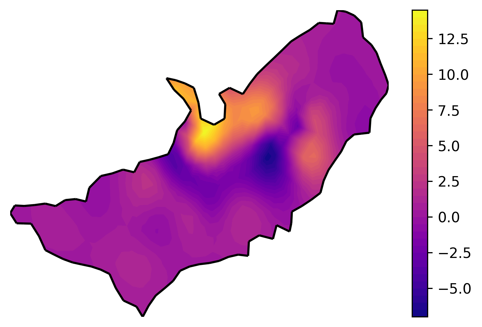
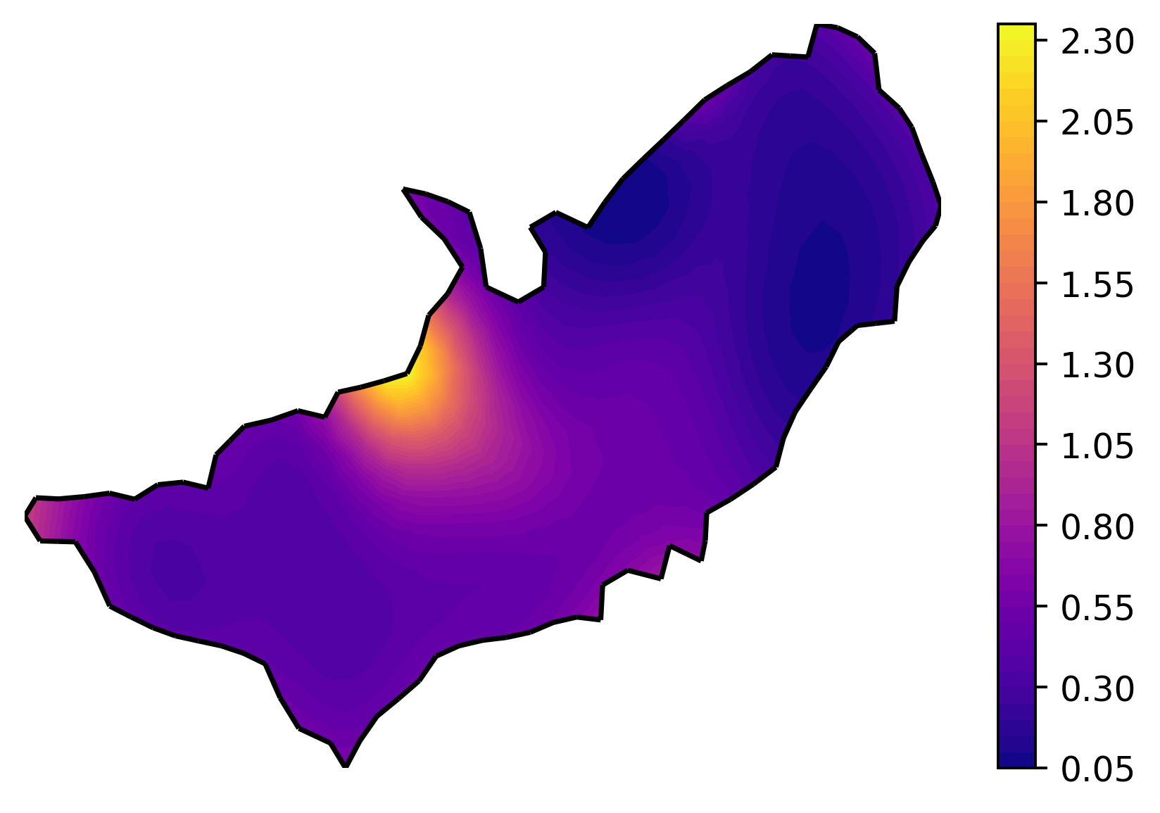
Our physically informed model is able to therefore learn a mechanism and so carry out sensible extrapolation, but this does not come at the expense of unrealistic prior restrictions, noteably when looking at the learned source function Fig. 13(b) we see that away from the data the source estimate is zero, and a similar observation can be made from the learned diffusion coefficient Fig. 13(c). By fitting a mechanistic model we learn parameters that fit the training data, avoid unrealistic prior assumptions, but crucially lead to region-wide generalisation. This is contrasted with the ground water level predictions from the mechanism free GP model in Fig. 14, which over-trains on the well locations and possesses no mechanism by which to regularise this behaviour.

(a) Well locations and regional mesh

(b) Mean source, $\mathbb{E}_{q(\mathbf{f})}[f(\mathbf{x})]$

(c) Mean diffusion coefficient, $\mathbb{E}_{q(\mathbf{g})}[e^{g(\mathbf{x})}]$

Figure 13: Additional figures for the aquifer experiment. (a) displays the locations of the training and test well sites. (b) presents the mean of the source from our GP-DT, and (c) presents the mean diffusion coefficient

(a) GP predicted ground water level

(b) GP-DT predicted ground water level

Figure 14: Additional ground water prediction figures for the aquifer experiment

References

- Abadi et al. [2015] Martín Abadi, Ashish Agarwal, Paul Barham, Eugene Brevdo, Zhifeng Chen, Craig Citro, Greg S. Corrado, Andy Davis, Jeffrey Dean, Matthieu Devin, Sanjay Ghemawat, Ian Goodfellow, Andrew Harp, Geoffrey Irving, Michael Isard, Yangqing Jia, Rafal Jozefowicz, Lukasz Kaiser, Manjunath Kudlur, Josh Levenberg, Dandelion Mané, Rajat Monga, Sherry Moore, Derek Murray, Chris Olah, Mike Schuster, Jonathon Shlens, Benoit Steiner, Ilya Sutskever, Kunal Talwar, Paul Tucker, Vincent Vanhoucke, Vijay Vasudevan, Fernanda Viégas, Oriol Vinyals, Pete Warden, Martin Wattenberg, Martin Wicke, Yuan Yu, and Xiaoqiang Zheng. TensorFlow: Large-scale machine learning on heterogeneous systems, 2015. URL https://www.tensorflow.org/. Software available from tensorflow.org.
- Ackerman et al. [2010] Daniel J. Ackerman, U. S. Geological Survey, Joseph P. Rousseau, Gordon W. Rattray, and Jason C. Fisher. Steady-state and transient models of groundwater flow and advective transport, eastern snake river plain aquifer, idaho national laboratory and vicinity, idaho. Technical report, USGS, 2010. URL http://pubs.er.usgs.gov/publication/sir20105123.
- Álvarez et al. [2009] Mauricio Álvarez, David Luengo, and Neil D. Lawrence. Latent force models. In David van Dyk and Max Welling, editors, Proceedings of the Twelth International Conference on Artificial Intelligence and Statistics, volume 5 of Proceedings of Machine Learning Research, pages 9–16, Hilton Clearwater Beach Resort, Clearwater Beach, Florida USA, 16–18 Apr 2009. PMLR. URL http://proceedings.mlr.press/v5/alvarez09a.html.
- Berg and Nyström [2017] Jens Berg and Kaj Nyström. A unified deep artificial neural network approach to partial differential equations in complex geometries, 2017.
- Brenner and Scott [2008] Sussanne Brenner and Ridgway Scott. The Mathematical theory of Finite Element Methods. Springer, New York, 2008.
- Brezis [2010] Haim Brezis. Functional Analysis, Sobolev Spaces and Partial Differential Equations. Springer, New York, 2010.
- Calderhead et al. [2009] Ben Calderhead, Mark Girolami, and Neil D. Lawrence. Accelerating bayesian inference over nonlinear differential equations with gaussian processes. In D. Koller, D. Schuurmans, Y. Bengio, and L. Bottou, editors, Advances in Neural Information Processing Systems 21, pages 217–224. Curran Associates, Inc., 2009. URL http://papers.nips.cc/paper/3497-accelerating-bayesian-inference-over-nonlinear-differential-equations-with-gaussian-processes.pdf.
- Chou and Voit [2009] I.-C. Chou and E. O. Voit. Recent developments in parameter estimation and structure identification of biochemical and genomic systems. Mathematical biosciences, 219(2):57 – 83, 2009.
- Cohen et al. [2019] Taco Cohen, Maurice Weiler, Berkay Kicanaoglu, and Max Welling. Gauge equivariant convolutional networks and the icosahedral CNN. In Kamalika Chaudhuri and Ruslan Salakhutdinov, editors, Proceedings of the 36th International Conference on Machine Learning, volume 97 of Proceedings of Machine Learning Research, pages 1321–1330, Long Beach, California, USA, 09–15 Jun 2019. PMLR. URL http://proceedings.mlr.press/v97/cohen19d.html.
- Cranmer et al. [2019] Kyle Cranmer, Johann Brehmer, and Gilles Louppe. The frontier of simulation-based inference, 2019.
- Damianou and Lawrence [2013] Andreas Damianou and Neil Lawrence. Deep gaussian processes. In Carlos M. Carvalho and Pradeep Ravikumar, editors, Proceedings of the Sixteenth International Conference on Artificial Intelligence and Statistics, volume 31 of Proceedings of Machine Learning Research, pages 207–215, Scottsdale, Arizona, USA, 29 Apr–01 May 2013. PMLR. URL http://proceedings.mlr.press/v31/damianou13a.html.
- Dattner and Klaassen [2015] Itai Dattner and Chris A. J. Klaassen. Optimal rate of direct estimators in systems of ordinary differential equations linear in functions of the parameters. Electron. J. Statist., 9(2):1939–1973, 2015. doi: 10.1214/15-EJS1053. URL https://doi.org/10.1214/15-EJS1053.
- de Bezenac et al. [2018] Emmanuel de Bezenac, Arthur Pajot, and Patrick Gallinari. Deep learning for physical processes: Incorporating prior scientific knowledge. In International Conference on Learning Representations, 2018. URL https://openreview.net/forum?id=By4HsfWAZ.
- Duane et al. [1987] Simon Duane, A.D. Kennedy, Brian J. Pendleton, and Duncan Roweth. Hybrid monte carlo. Physics Letters B, 195(2):216 – 222, 1987. ISSN 0370-2693. doi: https://doi.org/10.1016/0370-2693(87)91197-X. URL http://www.sciencedirect.com/science/article/pii/037026938791197X.
- Furrer et al. [2006] Reinhard Furrer, Marc G Genton, and Douglas Nychka. Covariance tapering for interpolation of large spatial datasets. Journal of Computational and Graphical Statistics, 15(3):502–523, 2006. doi: 10.1198/106186006X132178. URL https://doi.org/10.1198/106186006X132178.
- Gaspari and Cohn [1999] Gregory Gaspari and Stephen E. Cohn. Construction of correlation functions in two and three dimensions. Quarterly Journal of the Royal Meteorological Society, 125(554):723–757, 1999. doi: 10.1002/qj.49712555417. URL https://rmets.onlinelibrary.wiley.com/doi/abs/10.1002/qj.49712555417.
- Girolami et al. [2019] Mark Girolami, Alastair Gregory, Ge Yin, and Fehmi Cirak. The statistical finite element method, 2019.
- Goovaerts [1997] Pierre Goovaerts. Geostatistics for Natural Resources Evaluation. Oxford University Press, Oxford, 1997.
- Gorbach et al. [2017] Nico S Gorbach, Stefan Bauer, and Joachim M Buhmann. Scalable variational inference for dynamical systems. In I. Guyon, U. V. Luxburg, S. Bengio, H. Wallach, R. Fergus, S. Vishwanathan, and R. Garnett, editors, Advances in Neural Information Processing Systems 30, pages 4806–4815. Curran Associates, Inc., 2017. URL http://papers.nips.cc/paper/7066-scalable-variational-inference-for-dynamical-systems.pdf.
- Gupta and Meek [1996] K. K. Gupta and J. L. Meek. A brief history of the beginning of the finite element method. International Journal for Numerical Methods in Engineering, 39(22):3761–3774, 1996. doi: 10.1002/(SICI)1097-0207(19961130)39:22<3761::AID-NME22>3.0.CO;2-5. URL https://onlinelibrary.wiley.com/doi/abs/10.1002/%28SICI%291097-0207%2819961130%2939%3A22%3C3761%3A%3AAID-NME22%3E3.0.CO%3B2-5.
- Hensman et al. [2015] James Hensman, Alexander Matthews, and Zoubin Ghahramani. Scalable Variational Gaussian Process Classification. In Guy Lebanon and S. V. N. Vishwanathan, editors, Proceedings of the Eighteenth International Conference on Artificial Intelligence and Statistics, volume 38 of Proceedings of Machine Learning Research, pages 351–360, San Diego, California, USA, 09–12 May 2015. PMLR. URL http://proceedings.mlr.press/v38/hensman15.html.
- Ito and Kunisch [1990] K. Ito and K. Kunisch. The augmented Lagrangian method for parameter estimation in elliptic systems. SIAM Journal on Control and Optimisation, 28(1):113–136, 1990.
- Kennedy and O’Hagan [2001] Marc C. Kennedy and Anthony O’Hagan. Bayesian calibration of computer models. Journal of the Royal Statistical Society: Series B (Statistical Methodology), 63(3):425–464, 2001. doi: 10.1111/1467-9868.00294. URL https://rss.onlinelibrary.wiley.com/doi/abs/10.1111/1467-9868.00294.
- Kersting et al. [2020] Hans Kersting, Nicholas Krämer, Martin Schiegg, Christian Daniel, Michael Tiemann, and Philipp Hennig. Differentiable likelihoods for fast inversion of ’likelihood-free’ dynamical systems, 2020.
- Kingma and Welling [2014] Diederik P. Kingma and Max Welling. Auto-encoding variational Bayes. ICLR, 2014.
- Lázaro-Gredilla and Figueiras-Vidal [2009] Miguel Lázaro-Gredilla and Aníbal Figueiras-Vidal. Inter-domain gaussian processes for sparse inference using inducing features. In Y. Bengio, D. Schuurmans, J. D. Lafferty, C. K. I. Williams, and A. Culotta, editors, Advances in Neural Information Processing Systems 22, pages 1087–1095. Curran Associates, Inc., 2009. URL http://papers.nips.cc/paper/3876-inter-domain-gaussian-processes-for-sparse-inference-using-inducing-features.pdf.
- Lindgren et al. [2011] Finn Lindgren, Håvard Rue, and Johan Lindström. An explicit link between gaussian fields and gaussian markov random fields: the stochastic partial differential equation approach. Journal of the Royal Statistical Society: Series B (Statistical Methodology), 73(4):423–498, 2011. doi: 10.1111/j.1467-9868.2011.00777.x. URL https://rss.onlinelibrary.wiley.com/doi/abs/10.1111/j.1467-9868.2011.00777.x.
- Márquez-Neila et al. [2017] Pablo Márquez-Neila, Mathieu Salzmann, and Pascal Fua. Imposing hard constraints on deep networks: Promises and limitations, 2017.
- Nocedal and Wright [2006] Jorge Nocedal and S. Wright. Numerical Optimization. Springer-Verlag, New York, 2006.
- Oates and Sullivan [2019] Chris J. Oates and T. J. Sullivan. A modern retrospective on probabilistic numerics. Statistical Computing, 29:1335–1351, 2019.
- Philipp Hennig and Girolami [2015] Michael A. Osborne Philipp Hennig and Mark Girolami. Probabilistic numerics and uncertainty in computations. Proceedings of the Royal Society A, 2015.
- Raissi et al. [2019] M. Raissi, P. Perdikaris, and G.E. Karniadakis. Physics-informed neural networks: A deep learning framework for solving forward and inverse problems involving nonlinear partial differential equations. Journal of Computational Physics, 378:686 – 707, 2019. ISSN 0021-9991. doi: https://doi.org/10.1016/j.jcp.2018.10.045. URL http://www.sciencedirect.com/science/article/pii/S0021999118307125.
- Raissi and Karniadakis [2017] Maziar Raissi and George Karniadakis. Machine learning of linear differential equations using gaussian processes. Journal of Computational Physics, 348, 01 2017. doi: 10.1016/j.jcp.2017.07.050.
- Raissi et al. [2017] Maziar Raissi, Paris Perdikaris, and George Em Karniadakis. Physics informed deep learning (part i): Data-driven solutions of nonlinear partial differential equations, 2017.
- Reddy [2005] J Reddy. An Introduction to the Finite Element Method. McGraw-Hill Education, New York, 2005.
- Rezende et al. [2014] Danilo Jimenez Rezende, Shakir Mohamed, and Daan Wierstra. Stochastic backpropagation and approximate inference in deep generative models. In Eric P. Xing and Tony Jebara, editors, Proceedings of the 31st International Conference on Machine Learning, volume 32 of Proceedings of Machine Learning Research, pages 1278–1286, Bejing, China, 22–24 Jun 2014. PMLR. URL http://proceedings.mlr.press/v32/rezende14.html.
- Rudin et al. [1992] Leonid I. Rudin, Stanley Osher, and Emad Fatemi. Nonlinear total variation based noise removal algorithms. Physica D: Nonlinear Phenomena, 60(1):259 – 268, 1992. ISSN 0167-2789. doi: https://doi.org/10.1016/0167-2789(92)90242-F. URL http://www.sciencedirect.com/science/article/pii/016727899290242F.
- Salimbeni and Deisenroth [2017] Hugh Salimbeni and Marc Deisenroth. Doubly stochastic variational inference for deep gaussian processes. In I. Guyon, U. V. Luxburg, S. Bengio, H. Wallach, R. Fergus, S. Vishwanathan, and R. Garnett, editors, Advances in Neural Information Processing Systems 30, pages 4588–4599. Curran Associates, Inc., 2017. URL http://papers.nips.cc/paper/7045-doubly-stochastic-variational-inference-for-deep-gaussian-processes.pdf.
- Sirignano and Spiliopoulos [2018] Justin Sirignano and Konstantinos Spiliopoulos. Dgm: A deep learning algorithm for solving partial differential equations. Journal of Computational Physics, 375:1339 – 1364, 2018. ISSN 0021-9991. doi: https://doi.org/10.1016/j.jcp.2018.08.029. URL http://www.sciencedirect.com/science/article/pii/S0021999118305527.
- Solin and Kok [2019] Arno Solin and Manon Kok. Know your boundaries: Constraining gaussian processes by variational harmonic features. In Kamalika Chaudhuri and Masashi Sugiyama, editors, Proceedings of Machine Learning Research, volume 89 of Proceedings of Machine Learning Research, pages 2193–2202. PMLR, 16–18 Apr 2019. URL http://proceedings.mlr.press/v89/solin19a.html.
- Stein [1999] Michael L. Stein. Predicting random fields with increasing dense observations. Ann. Appl. Probab., 9(1):242–273, 02 1999. doi: 10.1214/aoap/1029962604. URL https://doi.org/10.1214/aoap/1029962604.
- Stuart [2010] Andrew M. Stuart. Inverse problems: A Bayesian perspective. Acta Numerica, 19:451–559, 2010.
- Voit [2000] E. O. Voit. Computational analysis of biochemical systems: A practical guide. Cambridge University Press, 2000.
- Wang et al. [2019] Rui Wang, Karthik Kashinath, Mustafa Mustafa, Adrian Albert, and Rose Yu. Towards physics-informed deep learning for turbulent flow prediction, 2019.
- Weiler and Cesa [2019] Maurice Weiler and Gabriele Cesa. General e(2)-equivariant steerable cnns. In H. Wallach, H. Larochelle, A. Beygelzimer, F. d’ Alché-Buc, E. Fox, and R. Garnett, editors, Advances in Neural Information Processing Systems 32, pages 14334–14345. Curran Associates, Inc., 2019. URL http://papers.nips.cc/paper/9580-general-e2-equivariant-steerable-cnns.pdf.
- Yazdani et al. [2019] Alireza Yazdani, Maziar Raissi, and George Em Karniadakis. Systems biology informed deep learning for inferring parameters and hidden dynamics. bioRxiv, 2019. doi: 10.1101/865063. URL https://www.biorxiv.org/content/early/2019/12/04/865063.
- Zellner [1988] Arnold Zellner. Optimal information processing and Bayes’s theorem. The American Statistician, 42(4):278–280, 1988. ISSN 00031305. URL http://www.jstor.org/stable/2685143.
- Zhu et al. [2019] Yinhao Zhu, Nicholas Zabaras, P. Koutsourelakis, and Paris Perdikaris. Physics-constrained deep learning for high-dimensional surrogate modeling and uncertainty quantification without labeled data. Journal of Computational Physics, 394, 05 2019. doi: 10.1016/j.jcp.2019.05.024.