Deep Bayesian Quadrature Policy Optimization

Abstract

We study the problem of obtaining accurate policy gradient estimates using a finite number of samples. Monte-Carlo methods have been the default choice for policy gradient estimation, despite suffering from high variance in the gradient estimates. On the other hand, more sample efficient alternatives like Bayesian quadrature methods have received little attention due to their high computational complexity. In this work, we propose deep Bayesian quadrature policy gradient (DBQPG), a computationally efficient high-dimensional generalization of Bayesian quadrature, for policy gradient estimation. We show that DBQPG can substitute Monte-Carlo estimation in policy gradient methods, and demonstrate its effectiveness on a set of continuous control benchmarks. In comparison to Monte-Carlo estimation, DBQPG provides (i) more accurate gradient estimates with a significantly lower variance, (ii) a consistent improvement in the sample complexity and average return for several deep policy gradient algorithms, and, (iii) the uncertainty in gradient estimation that can be incorporated to further improve the performance.

1 Introduction

Policy gradient (PG) is a reinforcement learning (RL) approach that directly optimizes the agent’s policies by operating on the gradient of their expected return (Sutton et al. 2000; Baxter and Bartlett 2000). The use of deep neural networks for the policy class has recently demonstrated a series of success for PG methods (Lillicrap et al. 2015; Schulman et al. 2015) on high-dimensional continuous control benchmarks, such as MuJoCo (Todorov, Erez, and Tassa 2012). However, the derivation and analysis of the aforementioned methods mainly rely on access to the expected return and its true gradient. In general, RL agents do not have access to the true gradient of the expected return, i.e., the gradient of integration over returns; instead, they have access to its empirical estimate from sampled trajectories. Monte-Carlo (MC) sampling (Metropolis and Ulam 1949) is a widely used point estimation method for approximating this integration (Williams 1992). However, MC estimation returns high variance gradient estimates that are undesirably inaccurate, imposing a high sample complexity requirement for PG methods (Rubinstein 1969; Ilyas et al. 2018).

An alternate approach to approximate integrals in probabilistic numerics is Bayesian Quadrature (BQ) (O’Hagan 1991). Under mild regularity assumptions, BQ offers impressive empirical advances and strictly faster convergence rates (Kanagawa, Sriperumbudur, and Fukumizu 2016). Typically, the integrand in BQ is modeled using a Gaussian process (GP), such that the linearity of the integral operator provides a Gaussian posterior over the integral. In addition to a point estimate of the integral, BQ also quantifies the uncertainty in its estimation, a missing piece in MC methods.

In RL, the BQ machinery can be used to obtain a Gaussian approximation of the PG integral, by placing a GP prior over the action-value function. However, estimating the moments of this Gaussian approximation, i.e., the PG mean and covariance, requires the integration of GP’s kernel function, which, in general, does not have an analytical solution. Interestingly, Ghavamzadeh and Engel (2007) showed that the PG integral can be solved analytically when the GP kernel is an additive combination of an arbitrary state kernel and a fixed Fisher kernel. While the authors demonstrate a superior performance of BQ over MC using a small policy network on simple environments, their approach does not scale to large non-linear policies ($>1000$ trainable parameters) and high-dimensional domains.

Contribution 1: We propose deep Bayesian quadrature policy gradient (DBQPG), a BQ-based PG framework that extends Ghavamzadeh and Engel (2007) to high-dimensional settings, thus placing it in the context of contemporary deep PG algorithms. The proposed framework uses a GP to implicitly model the action-value function, and without explicitly constructing the action-value function, returns a Gaussian approximation of the policy gradient, represented by a mean vector (gradient estimate) and covariance (gradient uncertainty). Consequently, this framework can be used with an explicit critic network (different from implicit GP critic) to leverage the orthogonal benefits of actor-critic frameworks (Schulman et al. 2016).

The statistical efficiency of BQ, relative to MC estimation, depends on the compatibility between the GP kernel and the MDP’s action-value function. To make DBQPG robust to a diverse range of target MDPs, we choose a base kernel capable of universal approximation (e.g. RBF kernel), and augment its expressive power using deep kernel learning (Wilson et al. 2016). Empirically, DBQPG estimates gradients that are both much closer to the true gradient, and with much lower variance, when compared to MC estimation. Moreover, DBQPG is a linear-time program that leverages the recent advances in structured kernel interpolation (Wilson and Nickisch 2015) for computational efficiency and GPU acceleration for fast kernel learning (Gardner et al. 2018). Therefore, DBQPG can favorably substitute MC estimation subroutine in a variety of PG algorithms. Specifically, we show that replacing the MC estimation subroutine with DBQPG provides a significant improvement in the sample complexity and average return for vanilla PG (Sutton et al. 2000), natural policy gradient (NPG) (Kakade 2001) and trust region policy optimization (TRPO) (Schulman et al. 2015) algorithms on $7$ diverse MuJoCo domains.

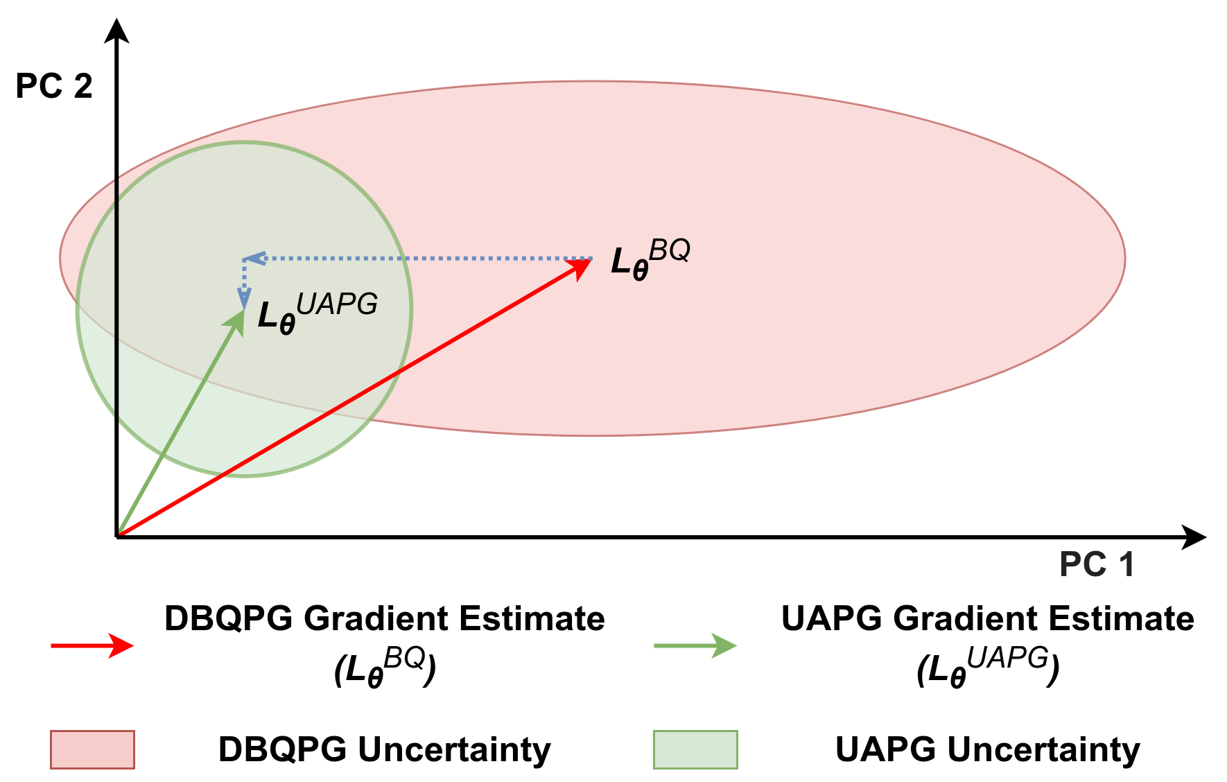
Contribution 2: We propose uncertainty aware PG (UAPG), a novel policy gradient method that utilizes the uncertainty in the gradient estimation for computing reliable policy updates. A majority of PG algorithms (Kakade 2001; Schulman et al. 2015) are derived assuming access to true gradients and therefore do not account the stochasticity in gradient estimation due to finite sample size. However, one can obtain more reliable policy updates by lowering the stepsize along the directions of high gradient uncertainty. UAPG captures this intuition by utilizing DBQPG’s uncertainty to bring different components of a stochastic gradient estimate to the same scale. UAPG does this by normalizing the step-size of the gradient components by their respective uncertainties, returning a new gradient estimate with uniform uncertainty, i.e., with new gradient covariance as the identity matrix. UAPG further provides a superior sample complexity and average return in comparison to DBQPG. Our implementation of DBQPG and UAPG methods is available online: https://github.com/Akella17/Deep-Bayesian-Quadrature-Policy-Optimization.

2 Preliminaries

Consider a Markov decision process (MDP) $\langle\mathcal{S},\mathcal{A},P,r,\rho_{0},\gamma\rangle$, where $\mathcal{S}$ is the state-space, $\mathcal{A}$ is the action-space, $P:\mathcal{S}\times\mathcal{A}\rightarrow\Delta_{\mathcal{S}}$ is the transition kernel that maps each state-action pair to a distribution over the states $\Delta_{\mathcal{S}}$, $r:\mathcal{S}\times\mathcal{A}\rightarrow\mathbb{R}$ is the reward kernel, $\rho_{0}:\Delta_{\mathcal{S}}$ is the initial state distribution, and $\gamma\in[0,1)$ is the discount factor. We denote by $\pi_{{\bm{\theta}}}:\mathcal{S}\rightarrow\Delta_{\mathcal{A}}$ a stochastic parameterized policy with parameters $\theta\in\Theta$. The MDP controlled by the policy $\pi_{{\bm{\theta}}}$ induces a Markov chain over state-action pairs $z=(s,a)\in\mathcal{Z}=\mathcal{S}\times\mathcal{A}$, with an initial density $\rho^{\pi_{{\bm{\theta}}}}_{0}(z_{0})=\pi_{{\bm{\theta}}}(a_{0}|s_{0})\rho_{0}(s_{0})$ and a transition probability distribution $P^{\pi_{{\bm{\theta}}}}(z_{t}|z_{t-1})=\pi_{{\bm{\theta}}}(a_{t}|s_{t})P(s_{t}|z_{t-1})$. We use the standard definitions for action-value function $Q_{\pi_{{\bm{\theta}}}}$ and expected return $J({\bm{\theta}})$ under $\pi_{{\bm{\theta}}}$:

$$Q_{\pi_{{\bm{\theta}}}}(z_{t})=\mathbb{E}\Bigg{[} \sum_{\tau=0}^{\infty}\gamma^{\tau}r(z_{t+\tau})~{}\Big{|}~{}z_{t+\tau+1}\sim P^{\pi_{{\bm{\theta}}}}(.|z_{t+\tau})\Bigg{]},$$

$$J({\bm{\theta}})=\mathbb{E}_{z_{0}\sim\rho^{\pi_{{\bm{\theta}}}}_{0}}\left[Q_{\pi_{{\bm{\theta}}}}(z_{0})\right].$$ (1)

However, the gradient of $J({\bm{\theta}})$ with respect to policy parameters ${\bm{\theta}}$ cannot be directly computed from this formulation. The policy gradient theorem (Sutton et al. 2000; Konda and Tsitsiklis 2000) provides an analytical expression for the gradient of the expected return $J({\bm{\theta}})$, as:

$$\displaystyle\nabla_{{\bm{\theta}}}J({\bm{\theta}}) =\int_{\mathcal{Z}}dz\rho^{\pi_{\bm{\theta}}}(z){\bm{u}}(z)Q_{\pi_{\bm{\theta}}}(z)$$

$$=\mathbb{E}_{z\sim\rho^{\pi_{\bm{\theta}}}}\big{[}{\bm{u}}(z)Q_{\pi_{\bm{\theta}}}(z)\big{]},$$ (2)

where ${\bm{u}}(z)=\nabla_{{\bm{\theta}}}\log\pi_{{\bm{\theta}}}(a|s)$ is the score function and $\rho^{\pi_{{\bm{\theta}}}}$ is the discounted state-action visitation frequency defined as:

$$\rho^{\pi_{{\bm{\theta}}}}(z) =\sum_{t=0}^{\infty}\gamma^{t}P^{\pi_{{\bm{\theta}}}}_{t}(z),\text{where}$$ (3)

$$P^{\pi_{{\bm{\theta}}}}_{t}(z_{t})=\int_{\mathcal{Z}^{t}}dz_{0}... dz_{t-1}P^{\pi_{{\bm{\theta}}}}_{0}(z_{0})\prod_{\tau=1}^{t}P^{\pi_{{\bm{\theta}}}}(z_{\tau}|z_{\tau-1}).$$

3 Policy Gradient Evaluation

The exact evaluation of the PG integral in Eq. 2 is often intractable for MDPs with a large (or continuous) state or action space. We discuss two prominent approaches to approximate this integral using a finite set of samples $\{z_{i}\}_{i=1}^{n}\sim\rho^{\pi_{\bm{\theta}}}$: (i) Monte-Carlo method and (ii) Bayesian Quadrature.

Monte-Carlo (MC) method approximates the integral in Eq. 2 by the finite sum:

$${\bm{L}}_{{\bm{\theta}}}^{MC}=\frac{1}{n}\sum_{i=1}^{n}Q_{\pi_{\bm{\theta}}}(z_{i}){\bm{u}}(z_{i})=\frac{1}{n}{\bm{U}}{\bm{Q}},$$ (4)

where ${\bm{u}}(z)$ is a $|\Theta|$ dimensional vector ($|\Theta|$ is the number of policy parameters). For conciseness, the function evaluations at sample locations $\{z_{i}\}_{i=1}^{n}\sim\rho^{\pi_{\bm{\theta}}}$ are grouped into ${\bm{U}}=[{\bm{u}}(z_{1}),...,{\bm{u}}(z_{n})]$, a $|\Theta|\times n$ dimensional matrix, and ${\bm{Q}}=[Q_{\pi_{\bm{\theta}}}(z_{1}),...,Q_{\pi_{\bm{\theta}}}(z_{n})]$, an $n$ dimensional vector. MC method returns the gradient mean evaluated at sample locations, which, according to the central limit theorem (CLT), is an unbiased estimate of the true gradient. However, CLT also suggests that the MC estimates suffer from a slow convergence rate ($n^{-1/2}$) and high variance, necessitating a large sample size $n$ for reliable PG estimation (Ilyas et al. 2018). Yet, MC methods are more computationally efficient than their sample-efficient alternatives (e.g. BQ), making them ubiquitous in PG algorithms.

Bayesian quadrature (BQ) (O’Hagan 1991) is an approach from probabilistic numerics (Hennig, Osborne, and Girolami 2015) that converts numerical integration into a Bayesian inference problem. The first step in BQ is to formulate a prior stochastic model over the integrand. This is done by placing a Gaussian process (GP) prior on the $Q_{\pi_{\bm{\theta}}}$ function, i.e., a mean zero GP $\mathbb{E}\left[Q_{\pi_{\bm{\theta}}}(z)\right]=0$, with a covariance function $k(z_{p},z_{q})=\mathrm{Cov}[Q_{\pi_{\bm{\theta}}}(z_{p}),Q_{\pi_{\bm{\theta}}}(z_{q})]$, and observation noise $\sigma$. Next, the GP prior on $Q_{\pi_{\bm{\theta}}}$ is conditioned (Bayes rule) on the sampled data $\mathcal{D}=\{z_{i}\}_{i=1}^{n}$ to obtain the posterior moments $\mathbb{E}\left[Q_{\pi_{\bm{\theta}}}(z)|\mathcal{D}\right]$ and $\mathcal{C}_{Q}(z_{1},z_{2})=\mathrm{Cov}\left[Q_{\pi_{\bm{\theta}}}(z_{1}),Q_{\pi_{\bm{\theta}}}(z_{2})|\mathcal{D}\right]$. Since the transformation from $Q_{\pi_{\bm{\theta}}}(z)$ to $\nabla_{{\bm{\theta}}}J({\bm{\theta}})$ happens through a linear integral operator (in Eq. 2), $\nabla_{{\bm{\theta}}}J({\bm{\theta}})$ also follows a Gaussian distribution:

$$\displaystyle{\bm{L}}_{{\bm{\theta}}}^{BQ} =\mathbb{E}\left[\nabla_{{\bm{\theta}}}J({\bm{\theta}})|\mathcal{D}\right]=\displaystyle\int_{\mathcal{Z}}dz\rho^{\pi_{\bm{\theta}}}(z){\bm{u}}(z)\mathbb{E}\left[Q_{\pi_{\bm{\theta}}}(z)|\mathcal{D}\right]$$

$$\displaystyle{\bm{C}}_{{\bm{\theta}}}^{BQ} =\mathrm{Cov}[\nabla_{{\bm{\theta}}}J({\bm{\theta}})|\mathcal{D}]$$ (5)

$$= \displaystyle\int_{\mathcal{Z}^{2}}dz_{1}dz_{2}\rho^{\pi_{\bm{\theta}}}(z_{1})\rho^{\pi_{\bm{\theta}}}(z_{2}){\bm{u}}(z_{1})\mathcal{C}_{Q}(z_{1},z_{2}){\bm{u}}(z_{2})^{\top},$$

where the mean vector ${\bm{L}}_{{\bm{\theta}}}^{BQ}$ is the PG estimate and the covariance ${\bm{C}}_{{\bm{\theta}}}^{BQ}$ is its uncertainty estimation. While the integrals in Eq. 3 are still intractable for an arbitrary GP kernel $k$, they have closed-form solutions when $k$ is the additive composition of a state kernel $k_{s}$ (arbitrary) and the Fisher kernel $k_{f}$ (indispensable) (Ghavamzadeh and Engel 2007):

$$k(z_{1},z_{2}) =c_{1}k_{s}(s_{1},s_{2})+c_{2}k_{f}(z_{1},z_{2}),$$

$$~{}~{}\textit{with}~{}k_{f} (z_{1},z_{2})={\bm{u}}(z_{1})^{\top}{\bm{G}}^{-1}{\bm{u}}(z_{2}),$$ (6)

where $c_{1},c_{2}$ are hyperparameters and ${\bm{G}}$ is the Fisher information matrix of $\pi_{\bm{\theta}}$. Using the matrices,

$${\bm{K}}_{f}={\bm{U}}^{\top}{\bm{G}}^{-1}{\bm{U}},\quad {\bm{K}}=c_{1}{\bm{K}}_{s}+c_{2}{\bm{K}}_{f},$$

$${\bm{G}}=\mathbb{E}_{z\sim\rho^{\pi_{\bm{\theta}}}}[{\bm{u}}(z) {\bm{u}}(z)^{\top}]\approx\frac{1}{n}{\bm{U}}{\bm{U}}^{\top},$$ (7)

the PG mean ${\bm{L}}_{{\bm{\theta}}}^{BQ}$ and covariance ${\bm{C}}_{{\bm{\theta}}}^{BQ}$ can be computed analytically (proof is deferred to the supplement Sec. B),

$$\displaystyle{\bm{L}}_{{\bm{\theta}}}^{BQ} =\displaystyle c_{2}{\bm{U}}({\bm{K}}+\sigma^{2}{\bm{I}})^{-1}{\bm{Q}},$$

$$\displaystyle{\bm{C}}_{{\bm{\theta}}}^{BQ} =c_{2}{\bm{G}}-c_{2}^{2}{\bm{U}}\left({\bm{K}}+\sigma^{2}{\bm{I}}\right)^{-1}{\bm{U}}^{\top}.$$ (8)

Here, ${\bm{Q}}$ is same as in the MC method. Note that removing the Fisher kernel $k_{f}$ (setting $c_{2}=0$ in Eq. 3) causes ${\bm{L}}_{{\bm{\theta}}}^{BQ}=0$ and ${\bm{C}}_{{\bm{\theta}}}^{BQ}=0$. Further, Ghavamzadeh and Engel (2007) showed that BQ-PG ${\bm{L}}_{{\bm{\theta}}}^{BQ}$ reduces to MC-PG ${\bm{L}}_{{\bm{\theta}}}^{MC}$ when the state kernel $k_{s}$ is removed ($c_{1}=0$).
To summarize, (i) the presence of Fisher kernel ($c_{2}\neq 0$) is essential for obtaining an analytical solution for BQ-PG, and (ii) with the Fisher kernel fixed, the choice of state kernel alone determines the convergence rate of BQ-PG relative to the MC baseline (equivalently BQ-PG with $c_{1}=0$).

4 Deep Bayesian Quadrature Policy Gradient

Here, we introduce the steps needed for obtaining a practical BQ-PG method, that (i) is more sample-efficient than MC baseline, and (ii) easily scales to high-dimensional settings.

Kernel Selection: In the previous section, it was highlighted that the flexibility of kernel selection is limited to the choice of the state kernel $k_{s}$. To understand the role of $k_{s}$, we first highlight the implication of the kernel composition proposed in Ghavamzadeh and Engel (2007). Specifically, the additive composition of the state kernel $k_{s}$ and the Fisher kernel $k_{f}$ implicitly divides the $Q_{\pi_{\bm{\theta}}}$ function into state-value function and advantage function, separately modeled by $k_{s}$ and $k_{f}$ respectively (supplement, Sec. C.1). Thus, removing the Fisher kernel $k_{f}$ ($c_{2}=0$) results in a non-existent advantage function, which explains ${\bm{L}}_{{\bm{\theta}}}^{BQ}=0$ and ${\bm{C}}_{{\bm{\theta}}}^{BQ}=0$. More interestingly, removing the state kernel $k_{s}$ ($c_{1}=0$) results in a non-existent state-value function, which also reduces ${\bm{L}}_{{\bm{\theta}}}^{BQ}$ to ${\bm{L}}_{{\bm{\theta}}}^{MC}$. In other words, MC-PG is a limiting case of BQ-PG where the state-value function is suppressed to $0$ (more details in the supplement Sec. C.2).

Thus, BQ-PG can offer more accurate gradient estimates than MC-PG, along with well-calibrated uncertainty estimates, when the state kernel $k_{s}$ is a better prior than the trivial $k_{s}=0$, for the MDP’s state-value function. To make the choice of $k_{s}$ robust to a diverse range of target MDPs, we suggest (i) a base kernel capable of universal approximation (e.g. RBF kernel), followed by (ii) increasing the base kernel’s expressive power by using a deep neural network (DNN) to transform its inputs (Wilson et al. 2016). Deep kernels combine the non-parametric flexibility of GPs with the structural properties of NNs to obtain more expressive kernel functions when compared to their base kernels. The kernel parameters $\bm{\phi}$ (DNN parameters + base kernel hyperparameters) are tuned using the gradient of GP’s log marginal likelihood $J_{GP}$ (Rasmussen and Williams 2005),

$$J_{GP}(\bm{\phi}|\mathcal{D})\propto\log|{\bm{K}}|-{\bm{Q}}^{\top}{\bm{K}}^{-1}{\bm{Q}},$$ (9)

$$\nabla_{\bm{\phi}}J_{GP} ={\bm{Q}}^{\top}{\bm{K}}^{-1}(\nabla_{\bm{\phi}}{\bm{K}}){\bm{K}}^{-1}{\bm{Q}}+Tr({\bm{K}}^{-1}\nabla_{\bm{\phi}}{\bm{K}}).$$

Figure 1: (Left) Overview of the DBQPG method, (Right) Illustration of DBQPG and UAPG updates along the first two principal components (PCs) of the gradient covariance matrix.

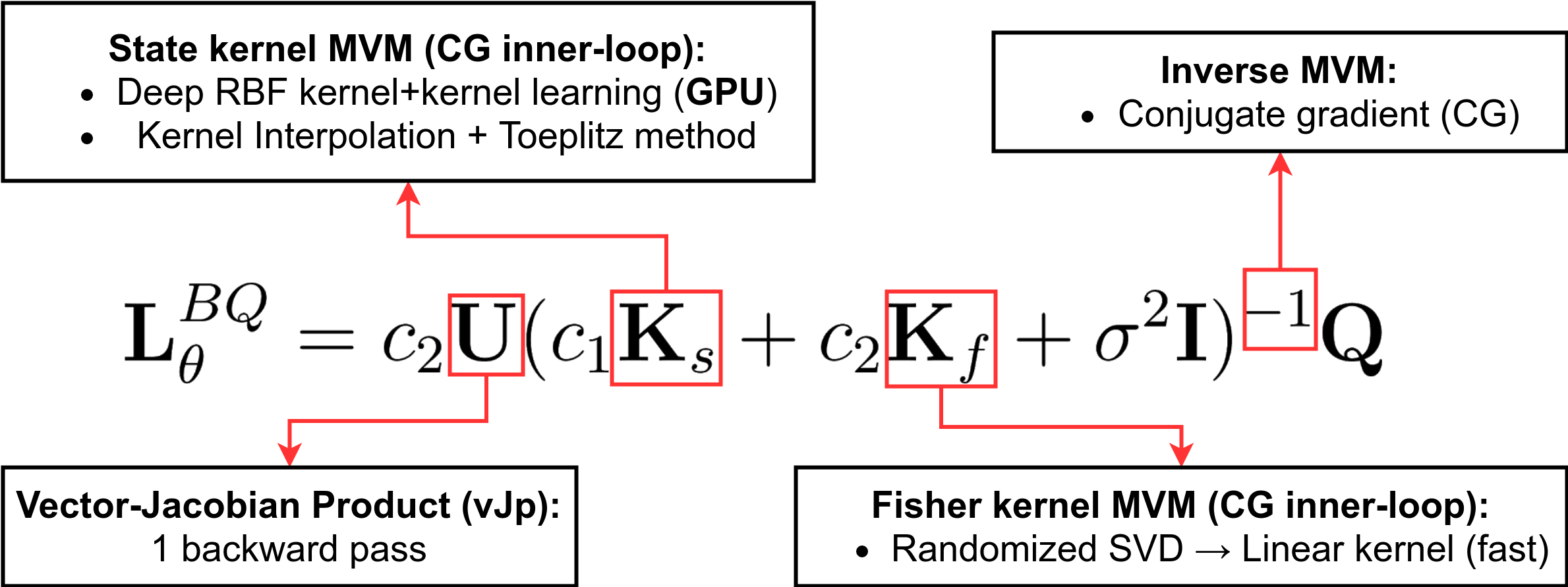
Scaling BQ to large sample sizes $n$: The complexity of estimating ${\bm{L}}_{{\bm{\theta}}}^{BQ}$ (Eq. 3) is largely influenced by the matrix-inversion operation $({\bm{K}}+\sigma^{2}{\bm{I}})^{-1}$, whose exact computation scales with an $\mathcal{O}(n^{3})$ time and $\mathcal{O}(n^{2})$ space complexity. Our first step is to shift the focus from an expensive matrix-inversion operation to an approximate inverse matrix-vector multiplication (i-MVM). In particular, we use the conjugate gradient (CG) method to compute the i-MVM $({\bm{K}}+\sigma^{2}{\bm{I}})^{-1}{\bm{v}}$ within machine precision using $p\ll n$ iterations of MVM operations ${\bm{K}}{\bm{v}}^{\prime}=c_{1}{\bm{K}}_{s}{\bm{v}}^{\prime}+c_{2}{\bm{K}}_{f}{\bm{v}}^{\prime}$.

While the CG method nearly reduces the time complexity by an order of $n$, the MVM operation with a dense matrix still incurs a prohibitive $\mathcal{O}(n^{2})$ computational cost. Fortunately, the matrix factorization of ${\bm{K}}_{f}$ (Eq. 3) allows for computing the Fisher kernel MVM ${\bm{K}}_{f}{\bm{v}}$ in linear-time through automatic differentiation, without the explicit creation or storage of the ${\bm{K}}_{f}$ matrix (more details in Sec. D.1 of the supplement). On the other hand, since the choice of $k_{s}$ is arbitrary, we deploy structured kernel interpolation (SKI) (Wilson and Nickisch 2015), a general kernel sparsification strategy to efficiently compute the state kernel MVM ${\bm{K}}_{s}{\bm{v}}$. SKI uses a set of $m\leq n$ “inducing points” $\{\hat{s}_{i}\}_{i=1}^{m}$ to approximate ${\bm{K}}_{s}$ with a rank $m$ matrix $\hat{{\bm{K}}}_{s}={\bm{W}}{\bm{K}}_{s}^{m}{\bm{W}}^{\top}$, where ${\bm{K}}_{s}^{m}$ is an $m\times m$ Gram matrix with entries ${{\bm{K}}_{s}^{m}}_{(p,q)}=k_{s}(\hat{s}_{p},\hat{s}_{q})$, and ${\bm{W}}$ is an $n\times m$ interpolation matrix whose entries depend on the relative placement of sample points $\{s_{i}\}_{i=1}^{n}$ and inducing points $\{\hat{s}_{i}\}_{i=1}^{m}$. In practice, a sparse ${\bm{W}}$ matrix that follows local cubic interpolation (only $4$ non-zero entries per row) provides a good approximation $\hat{{\bm{K}}}_{s}$, and more importantly, offers $\hat{{\bm{K}}}_{s}{\bm{v}}$ MVM in $\mathcal{O}(n+m^{2})$ time and storage complexity.

Further, the SKI framework also provides the flexibility to select the inducing point locations for exploiting the structure of specialized GP kernels. For instance, one-dimensional stationary kernels, i.e., $k_{s}(x,y)=k_{s}(x-y)$, can additionally leverage the Toeplitz method (Turner 2010) by picking evenly-spaced inducing points. Since these matrices are constant along the diagonal, i.e. ${{\bm{K}}_{s}}_{(x,y)}={{\bm{K}}_{s}}_{(x+1,y+1)}$, the Toeplitz method utilizes fast Fourier transform to attain an $\mathcal{O}(n+m\log m)$ time and $\mathcal{O}(n+m)$ storage for the MVM operation. Further, Toeplitz methods can be extended to multiple dimensions by assuming that the kernel decomposes as a sum of one-dimensional stationary kernels along each of the input dimensions. Compared to conventional inducing point methods that operate with $m\ll n$ inducing points, choosing a base kernel that conforms with the Toeplitz method enables the realization of larger $m$ values, thereby providing a more accurate approximation of ${\bm{K}}_{s}$.

Practical DBQPG Algorithm: The DBQPG algorithm is designed to compute the gradient from a batch of samples (parallelly) leveraging the automatic differentiation framework and fast kernel computation methods, thus placing BQ-PG in the context of contemporary PG algorithms (see Fig. 1(left)). In contrast, the original BQ-PG method (Ghavamzadeh and Engel 2007) was designed to process the samples sequentially (slow). Other major improvements in DBQPG include (i) replacing a traditional inducing points method ($\mathcal{O}(m^{2}n+m^{3})$ time and $\mathcal{O}(mn+m^{2})$ storage) with SKI, a more efficient alternative ($\mathcal{O}(n+m^{2})$ time and storage), and (ii) replacing a fixed base kernel for $k_{s}$ with the more expressive deep kernel, followed by learning the kernel parameters (Eq. 9). The performance gains from deep kernel learning and SKI are documented in supplement Sec. G.

For DBQPG, our default choice for the prior state covariance function $k_{s}$ is a deep RBF kernel which comprises of an RBF base kernel on top of a DNN feature extractor. Our choice of RBF as the base kernel is based on: (i) its compelling theoretical properties such as infinite basis expansion and universal function approximation (Micchelli, Xu, and Zhang 2006) and (ii) its compatibility with the Toeplitz method. Thus, the overall computational complexity of estimating ${\bm{L}}_{{\bm{\theta}}}^{BQ}$ (Eq. 3) is $\mathcal{O}(p(n+Ym\log m))$ time and $\mathcal{O}(n+Ym)$ storage ($Y$: state dimensionality; $p$: CG iterations; $m$: number of inducing points in SKI+Toeplitz approximation for a deep RBF kernel; automatic differentiation for Fisher kernel).

Note that we intentionally left out kernel learning from the complexity analysis since a naive implementation of the gradient-based optimization step (Eq. 9) incurs a cubic time complexity in sample size. Our implementation relies on the black-box matrix-matrix multiplication (BBMM) feature (a batched version of CG algorithm that effectively uses GPU hardware) offered by the GPyTorch library (Gardner et al. 2018), coupled with a SKI approximation over ${\bm{K}}_{s}$. This combination offers a linear-time routine for kernel learning. In other words, DBQPG with kernel learning is a linear-time program that leverages GPU acceleration to efficiently estimate the gradient of a large policy network, with a few thousands of parameters, on high-dimensional domains.

5 Uncertainty Aware Policy Gradient

We propose UAPG, a novel uncertainty aware PG method that utilizes the gradient uncertainty ${\bm{C}}_{{\bm{\theta}}}^{BQ}$ from DBQPG to provide more reliable policy updates. Most classical PG methods consider stochastic gradient estimates as the true gradient, without accounting the uncertainty in their gradient components, thus, occasionally taking large steps along the directions of high uncertainty. UAPG provides more reliable policy updates by lowering the stepsize along the directions with high uncertainty. In particular, UAPG uses ${\bm{C}}_{{\bm{\theta}}}^{BQ}$ to normalize the components of ${\bm{L}}_{{\bm{\theta}}}^{BQ}$ with their respective uncertainties, bringing them all to the same scale. Thus, UAPG offers PG estimates with a uniform uncertainty, i.e. their gradient covariance is the identity matrix. See Fig. 1 (right). In theory, the UAPG update can be formulated as $\big{(}{\bm{C}}_{{\bm{\theta}}}^{BQ}\big{)}^{-\frac{1}{2}}{\bm{L}}_{{\bm{\theta}}}^{BQ}$.

Practical UAPG Algorithm: Empirical ${\bm{C}}_{{\bm{\theta}}}^{BQ}$ estimates are often ill-conditioned matrices (spectrum decays quickly) with a numerically unstable inversion. Since ${\bm{C}}_{{\bm{\theta}}}^{BQ}$ only provides a faithful estimate of the top few principal directions of uncertainty, the UAPG update is computed from a rank-$\delta$ singular value decomposition (SVD) approximation of ${\bm{C}}_{{\bm{\theta}}}^{BQ}\approx\nu_{\delta}{\bm{I}}+\sum_{i=1}^{\delta}{\bm{h}}_{i}(\nu_{i}-\nu_{\delta}){\bm{h}}_{i}^{\top}$ as follows:

$${\bm{L}}_{{\bm{\theta}}}^{UAPG}=\nu_{\delta}^{-\frac{1}{2}}\big{(}{\bm{I}}+\sum_{i=1}^{\delta}{\bm{h}}_{i}\big{(}\sqrt{{\nu_{\delta}}/{\nu_{i}}}-1\big{)}{\bm{h}}_{i}^{\top}\big{)}{\bm{L}}_{{\bm{\theta}}}^{BQ}.$$ (10)

The principal components (PCs) $\{{\bm{h}}_{i}\}_{i=1}^{\delta}$ denote the top $\delta$ directions of uncertainty and the singular values $\{\nu_{i}\}_{i=1}^{\delta}$ denote their corresponding magnitudes of uncertainty. The rank-$\delta$ decomposition of ${\bm{C}}_{{\bm{\theta}}}^{BQ}$ can be computed in linear-time using the randomized SVD algorithm (Halko, Martinsson, and Tropp 2011). The UAPG update in Eq. 10 dampens the stepsize of the top $\delta$ directions of uncertainty, relative to the stepsize of remaining gradient components. Thus, in comparison to DBQPG, UAPG lowers the risk of taking large steps along the directions of high uncertainty, providing reliable policy updates.

For natural gradient ${\bm{L}}_{{\bm{\theta}}}^{NBQ}={\bm{G}}^{-1}{\bm{L}}_{{\bm{\theta}}}^{BQ}$, the gradient uncertainty can be computed as follows:

$${\bm{C}}_{{\bm{\theta}}}^{NBQ}={\bm{G}}^{-1}{\bm{C}}_{{\bm{\theta}}}^{BQ}{\bm{G}}^{-1}$$

$$=c_{2}{\bm{G}}^{-1}-c_{2}^{2}{\bm{G}}^{-1}{\bm{U}}\left(c_{1}{\bm{K}}_{s}+c_{2}{\bm{K}}_{f}+\sigma^{2}{\bm{I}}\right)^{-1}{\bm{U}}^{\top}{\bm{G}}^{-1}$$

$$=c_{2}({\bm{G}}+c_{2}{\bm{U}}\left(c_{1}{\bm{K}}_{s}+\sigma^{2}{\bm{I}}\right)^{-1}{\bm{U}}^{\top})^{-1}.$$ (11)

Since ${\bm{C}}_{{\bm{\theta}}}^{NBQ}$ is the inverse of an ill-conditioned matrix, we instead apply a low-rank approximation on ${{\bm{C}}_{{\bm{\theta}}}^{NBQ}}^{-1}\approx\nu_{\delta}{\bm{I}}+\sum_{i=1}^{\delta}{\bm{h}}_{i}(\nu_{i}-\nu_{\delta}){\bm{h}}_{i}^{\top}$ for the UAPG update of NPG:

$${\bm{L}}_{{\bm{\theta}}}^{NUAPG}=\nu_{\delta}^{\frac{1}{2}}\Big{(}{\bm{I}}+\sum_{i=1}^{\delta}{\bm{h}}_{i}\big{(}\min\big{(}\sqrt{\frac{\nu_{i}}{\nu_{\delta}}},{\epsilon}\big{)}-1\big{)}{\bm{h}}_{i}^{\top}\Big{)}{\bm{G}}^{-1}{\bm{L}}_{{\bm{\theta}}}^{BQ},$$ (12)

where, $\{{\bm{h}}_{i},\nu_{i}\}_{i=1}^{\delta}$ correspond to the top $\delta$ PCs of ${{\bm{C}}_{{\bm{\theta}}}^{NBQ}}^{-1}$ (equivalently the bottom $\delta$ PCs of ${\bm{C}}_{{\bm{\theta}}}^{NBQ}$), and ${\epsilon}>1$ is a hyperparameter. We replace $\sqrt{{\nu_{i}}/{\nu_{\delta}}}$ with $\min(\sqrt{{\nu_{i}}/{\nu_{\delta}}},{\epsilon})$ to avoid taking large steps along these directions, solely on the basis of their uncertainty estimates. For $c_{2}\ll 1$, it is interesting to note that (i) ${\bm{C}}_{{\bm{\theta}}}^{BQ}\approx c_{2}{\bm{G}}$ and ${\bm{C}}_{{\bm{\theta}}}^{NBQ}\approx c_{2}{\bm{G}}^{-1}$, which implies that the most uncertain gradient directions for vanilla PG approximately correspond to the most confident directions for NPG, and (ii) the ideal UAPG update for both vanilla PG and NPG converges along the ${\bm{G}}^{-\frac{1}{2}}{\bm{L}}_{{\bm{\theta}}}^{BQ}$ direction. A more rigorous discussion on the relations between Vanilla PG, NPG and their UAPG updates can be found in the supplement Sec. E.1.

Algorithm 1 BQ-PG Estimator Subroutine

1:BQ-PG(${\bm{\theta}},n$)

2:• ${\bm{\theta}}$: policy parameters

3:• $n$: sample size for PG estimation

4:Collect $n$ state-action pairs (samples) from running the policy $\pi_{{\bm{\theta}}}$ in the environment.

5:Compute action-values ${\bm{Q}}$ for these $n$ samples using MC rollouts (TD(1) estimate) or an explicit critic network.

6:Update kernel parameters and explicit critic’s parameters using GP MLL (Eq. 9) and TD error respectively.

7:Policy gradient estimation (DBQPG):

8:${\bm{L}}_{{\bm{\theta}}}=\begin{cases}{\bm{L}}_{{\bm{\theta}}}^{BQ}&\text{(Vanilla {PG})}\\ {\bm{G}}^{-1}{\bm{L}}_{{\bm{\theta}}}^{BQ}&\text{(Natural {PG})}\end{cases}$

9:(Optional) Compute $\{{\bm{h}}_{i},\nu_{i}\}_{i=1}^{\delta}$ using fast SVD over ${{\bm{C}}_{{\bm{\theta}}}^{BQ}}$ (Eq. 3, vanilla PG) or ${{\bm{C}}_{{\bm{\theta}}}^{NBQ}}^{-1}$ (Eq. 5, NPG).

10:(Optional) Uncertainty-based adjustment (UAPG):

11:${\bm{L}}_{{\bm{\theta}}}=\begin{cases}\nu_{\delta}^{-\frac{1}{2}}\left({\bm{I}}+\sum\limits_{i=1}^{\delta}{\bm{h}}_{i}\left(\sqrt{\frac{\nu_{\delta}}{\nu_{i}}}-1\right){\bm{h}}_{i}^{\top}\right){\bm{L}}_{{\bm{\theta}}}\\ \text{(Vanilla {PG})}\\ \nu_{\delta}^{\frac{1}{2}}\left({\bm{I}}+\sum\limits_{i=1}^{\delta}{\bm{h}}_{i}\left(\min\left(\sqrt{\frac{\nu_{i}}{\nu_{\delta}}},{\epsilon}\right)-1\right){\bm{h}}_{i}^{\top}\right){\bm{G}}^{-1}{\bm{L}}_{{\bm{\theta}}}\\ \text{(Natural {PG})}\end{cases}$

12:return ${\bm{L}}_{{\bm{\theta}}}$

6 Experiments

We study the behaviour of BQ-PG methods (Algorithm 1) on MuJoCo environments, using the mujoco-py library of OpenAI Gym (Brockman et al. 2016). In our experiments, we replace ${\bm{Q}}$ with generalized advantage estimates (Schulman et al. 2016) computed using an explicit state-value critic network, i.e., $V_{\pi_{{\bm{\theta}}}}(s)$ is approximated using a linear layer on top of the state feature extractor in Fig. 1(left).

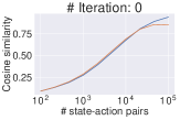
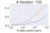
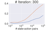
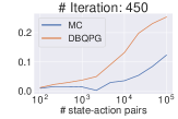
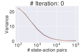
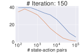
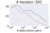
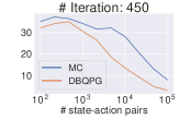
Quality of Gradient Estimation: Inspired from the experimental setup of Ilyas et al. (2018), we evaluate the quality of PG estimates obtained via DBQPG and MC estimation using two metrics: (i) gradient accuracy or the average cosine similarity of the obtained gradient estimates with respect to the true gradient estimates (estimated from $10^{6}$ state-action pairs) and (ii) variance in the gradient estimates (normalized by the norm of the mean gradient for scale invariance). See Fig. 2. We observe that DBQPG provides more accurate gradient estimates with a considerably lower variance. Interestingly, DBQPG and MC estimates offer nearly the same quality gradients at the start of training. However, as the training progresses, and DBQPG learns kernel bases, we observe that DBQPG returns superior quality gradient estimates. Moreover, as training progress from $0$ to $150$ iterations, the gradient norms of both DBQPG and MC estimates drop by a factor of $3$, while the “unnormalized” gradient variances increase by $5$ folds. The drop in the signal-to-noise ratio for gradient estimation explains the fall in accuracy over training time. Further, the wall-clock time of DBQPG and UAPG updates is comparable to MC-PG (Fig. 6 in supplement). These results motivate substituting MC with BQ-based PG estimates in deep PG algorithms.

Figure 2: An empirical analysis of the quality of policy gradient estimates as a function of the state-action sample size. The experiments are conducted for $0^{th}$, $150^{th}$, $300^{th}$, and $450^{th}$ iteration along the training phase of DBQPG (vanilla PG) algorithm in MuJoCo Swimmer-v2 environment. All the results have been averaged over $25$ repeated gradient measurements across $100$ random runs. (a) The accuracy plot results are obtained w.r.t the “true gradient”, which is computed using MC estimates of $10^{6}$ state-action pairs. (b) The normalized variance is computed using the ratio of trace of empirical gradient covariance matrix (like Zhao et al. (2011)) and squared norm of gradient mean.

Vanilla PG

NPG

TRPO

Figure 3: The average performance ($10$ runs) of BQ-based methods and MC estimation in vanilla PG, NPG, and TRPO frameworks across $4$ MuJoCo environments (refer Fig. 9 in the supplement for comparison across all $7$ MuJoCo environments).

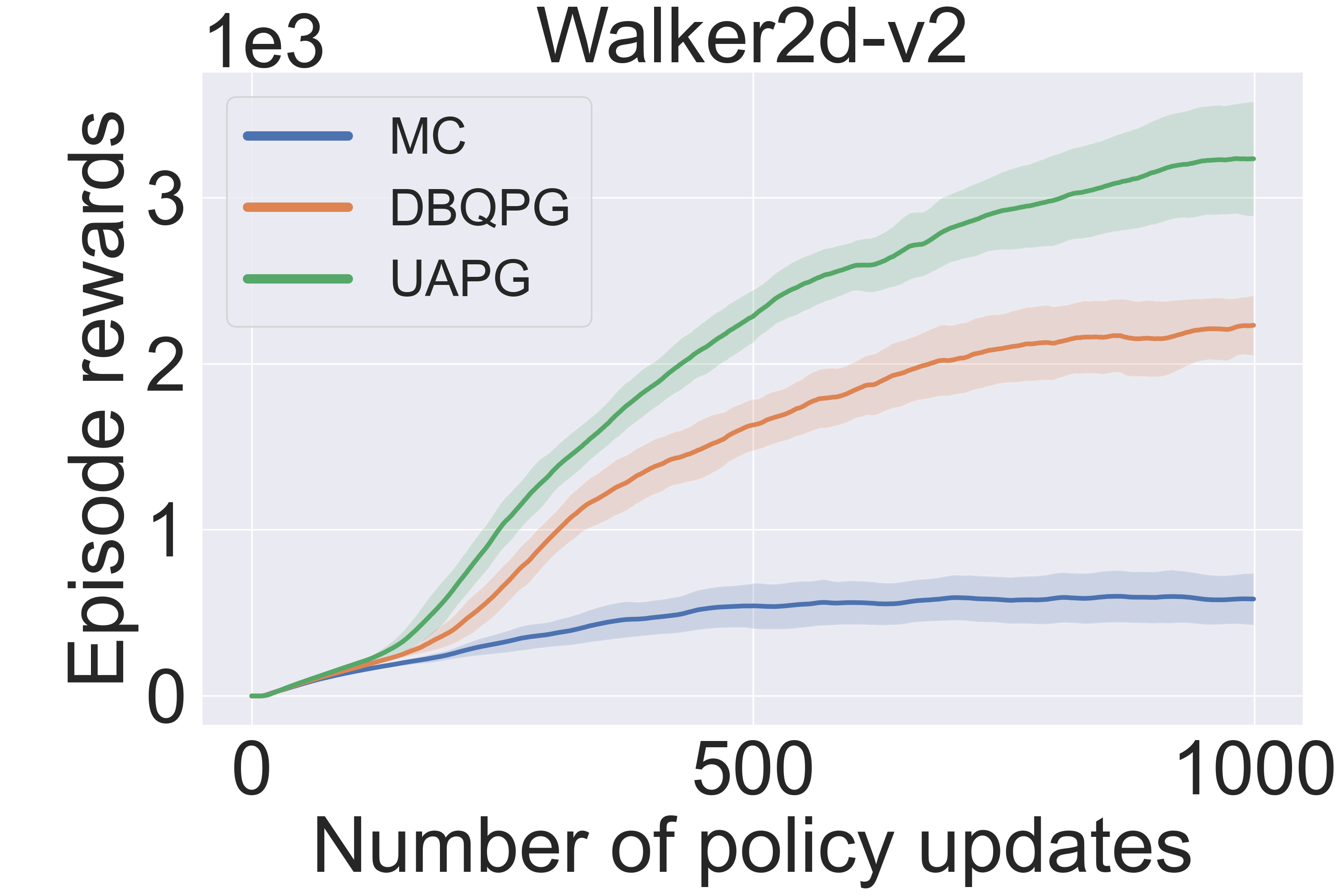
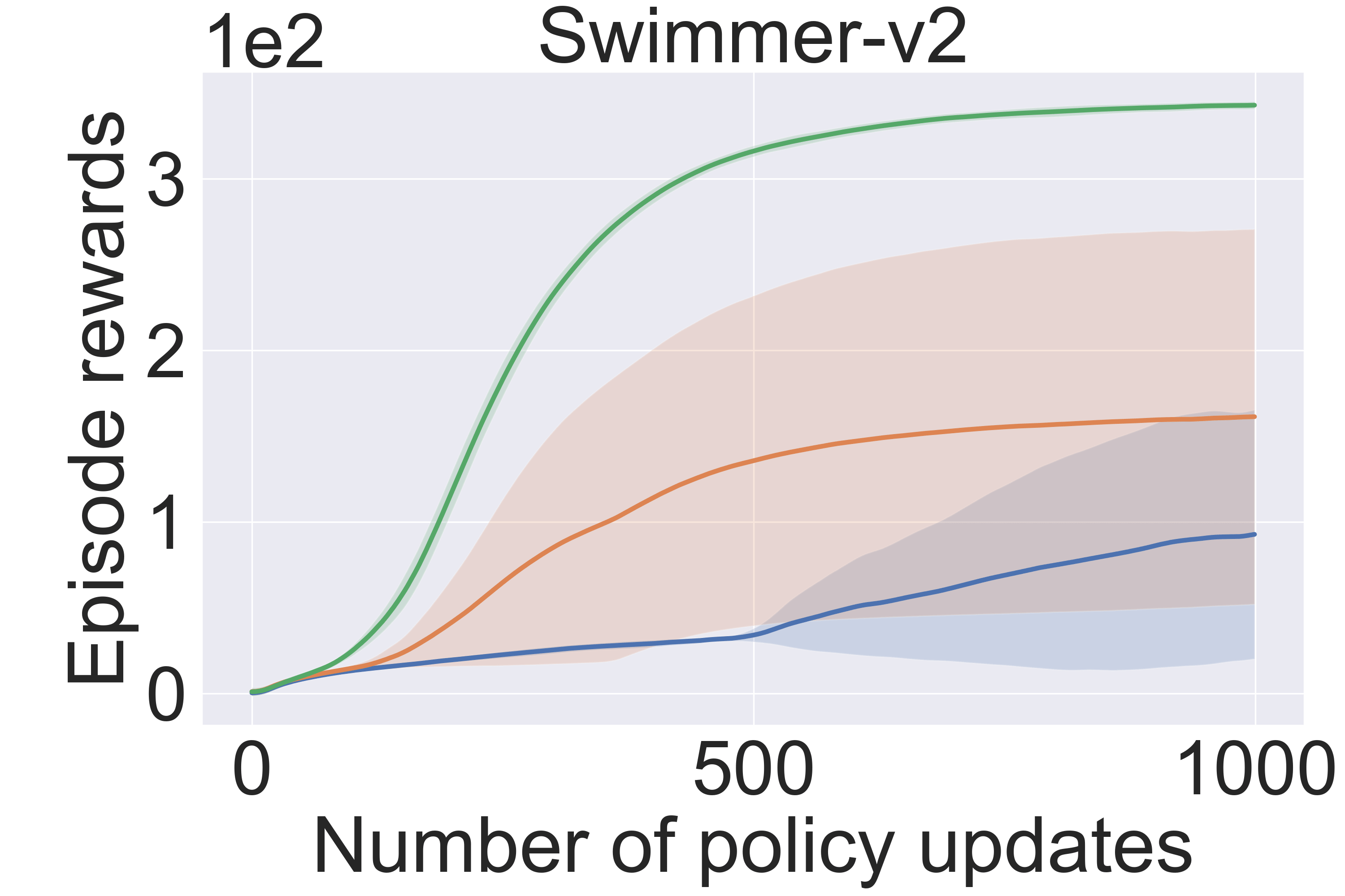
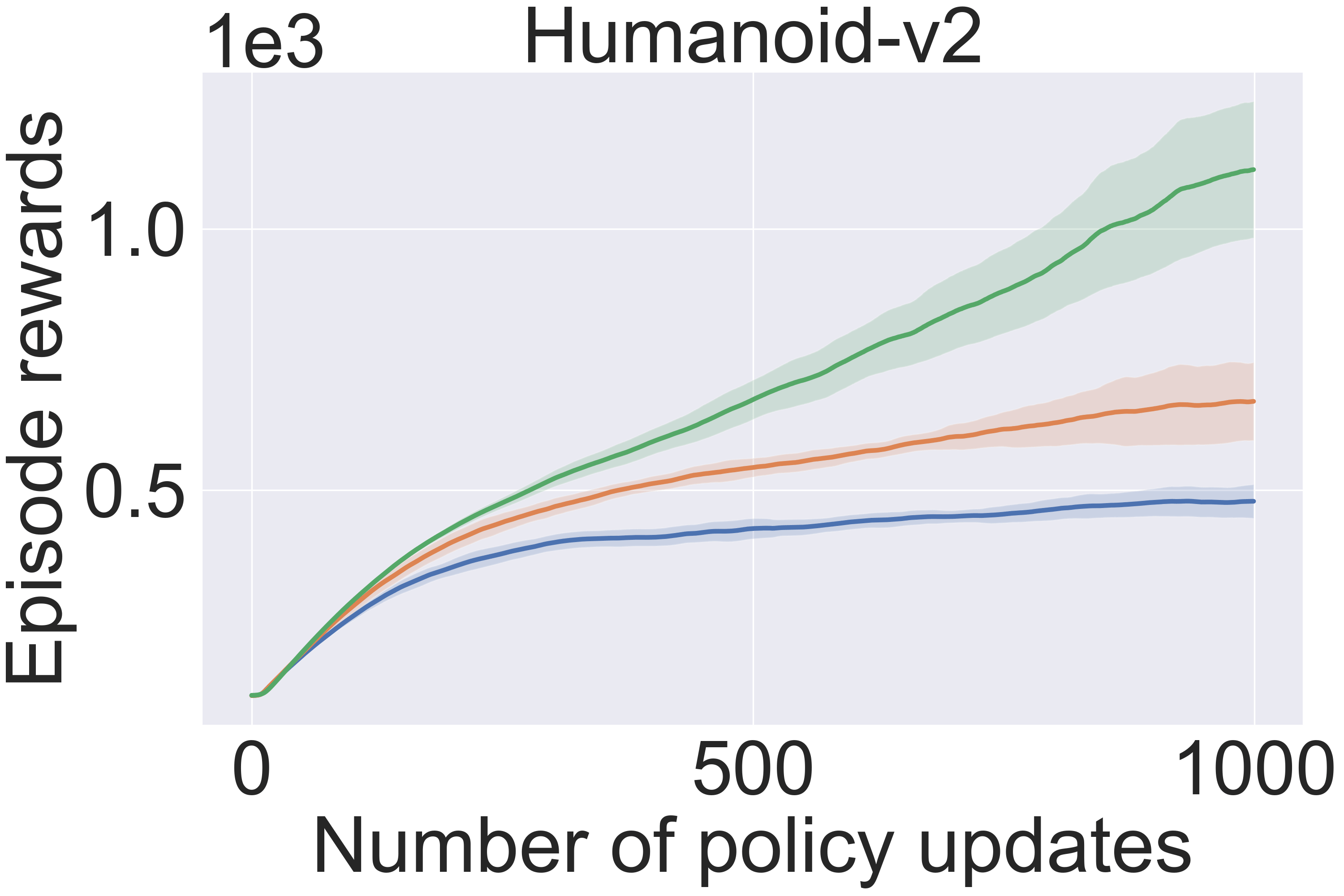
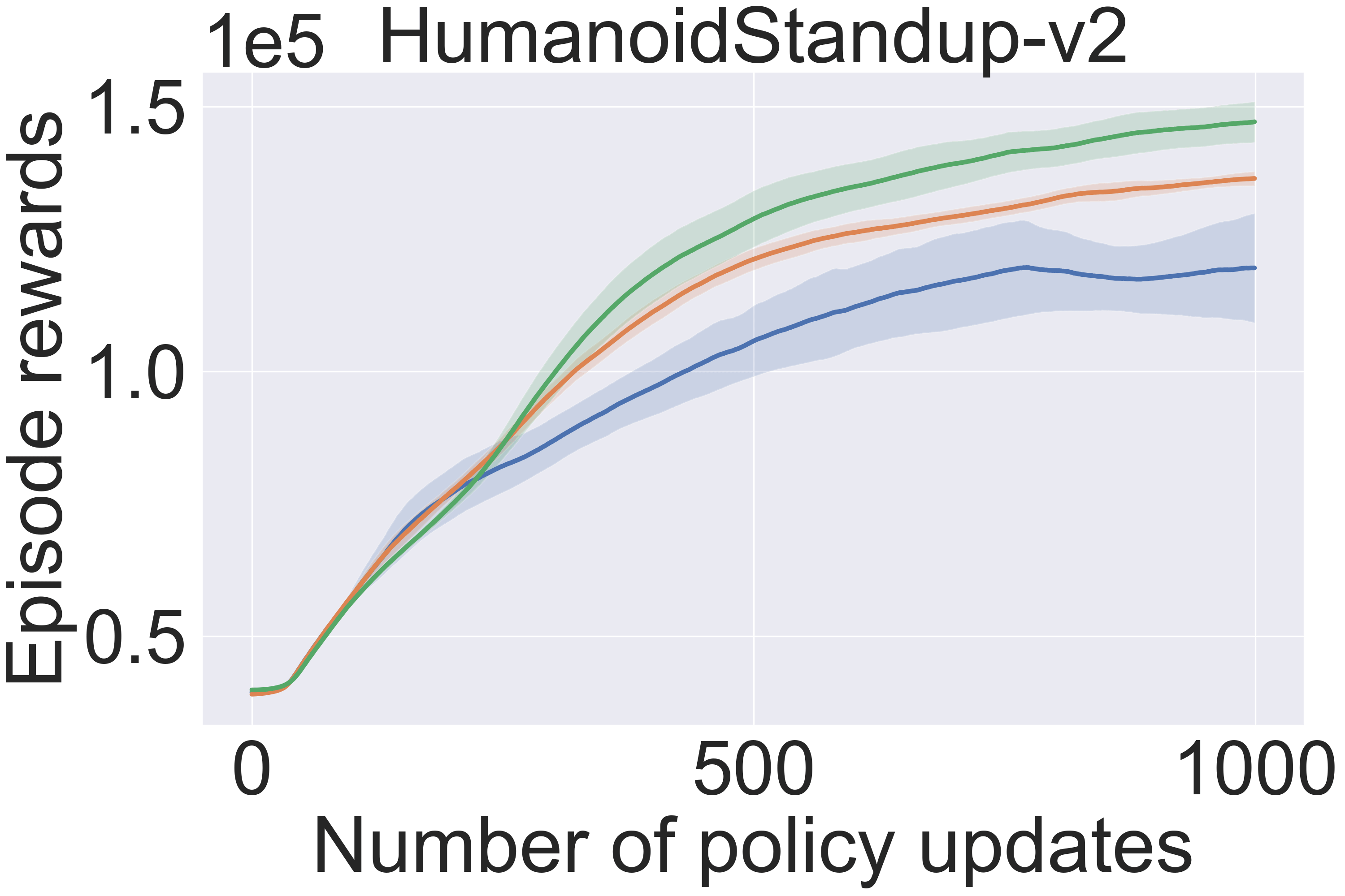
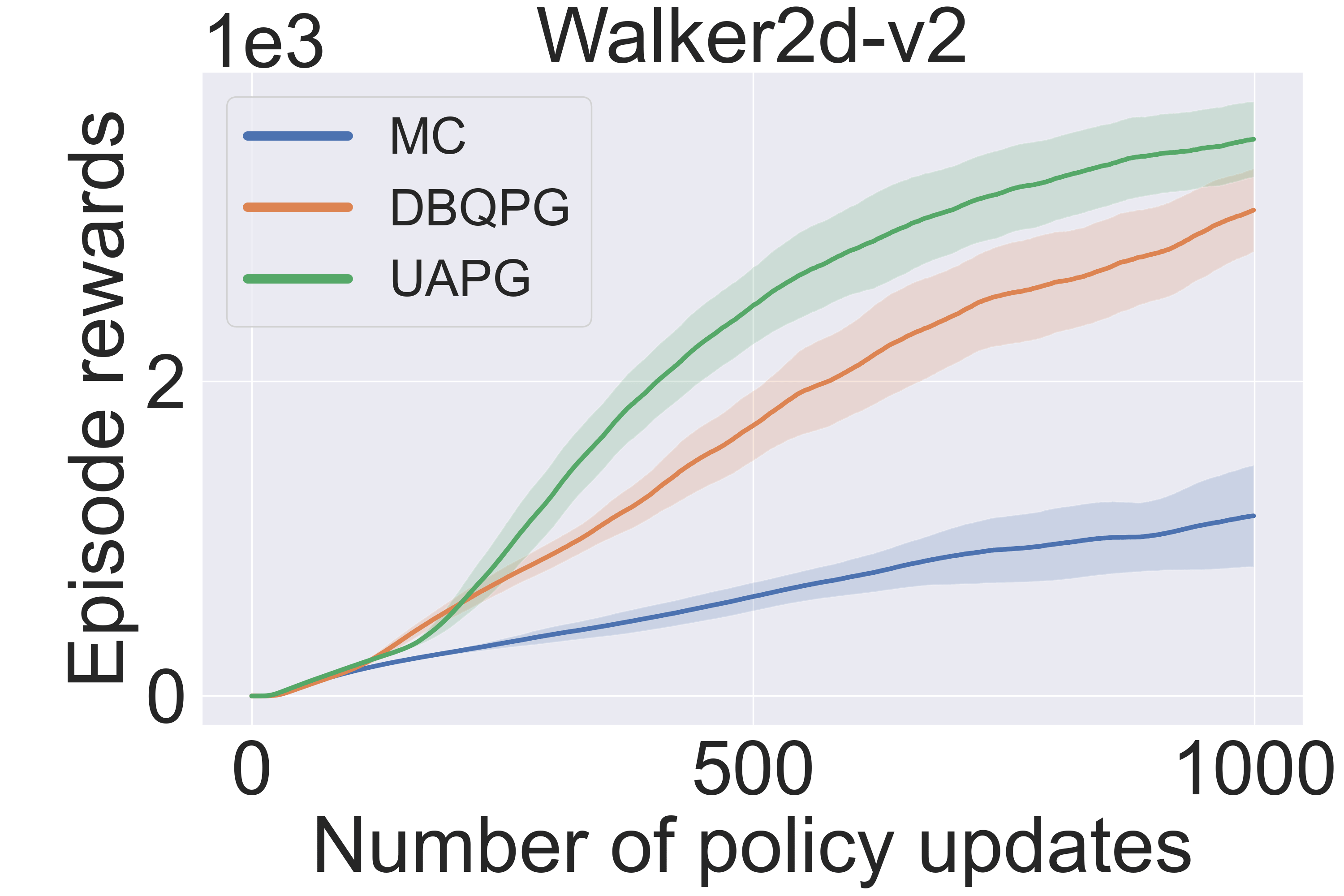
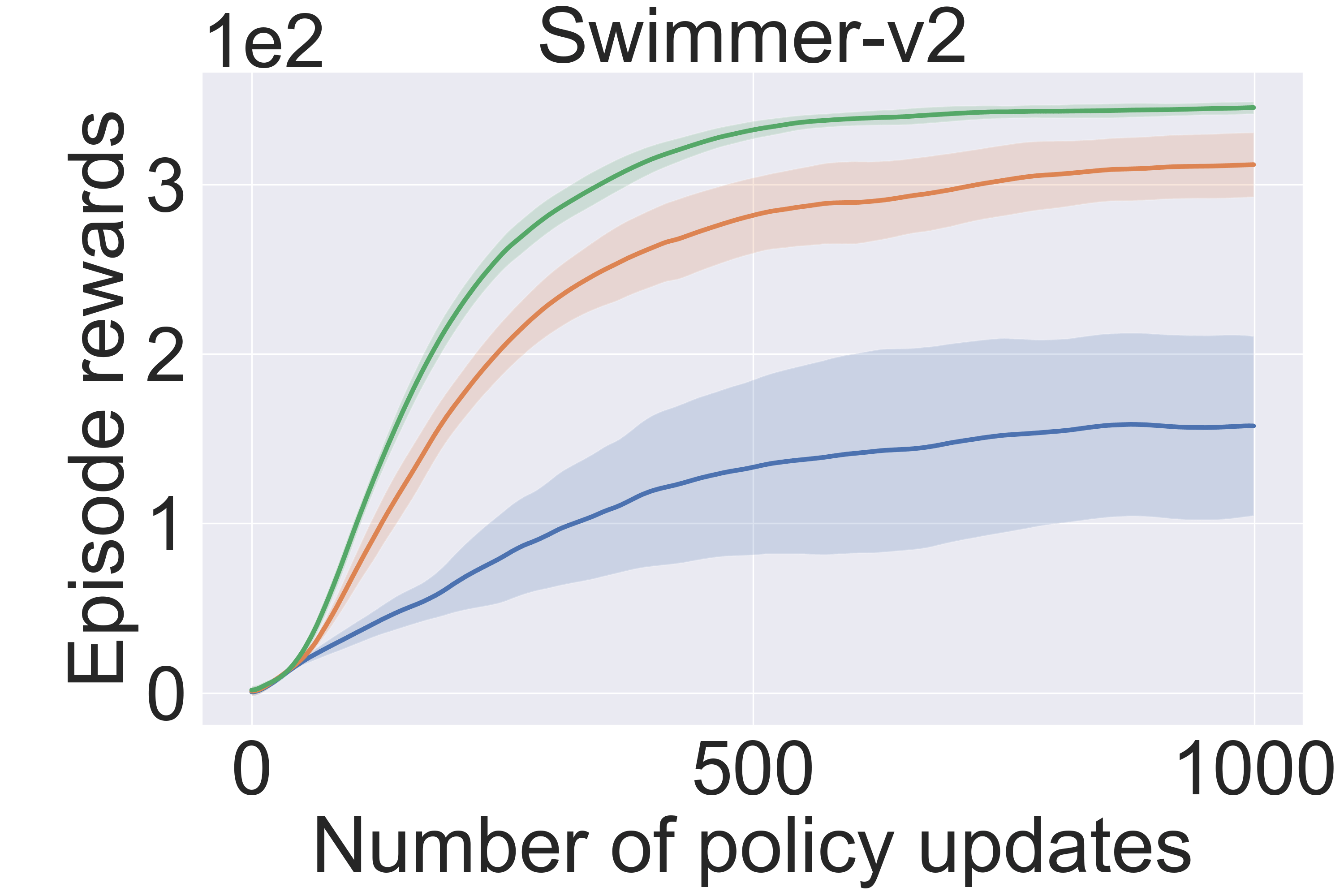
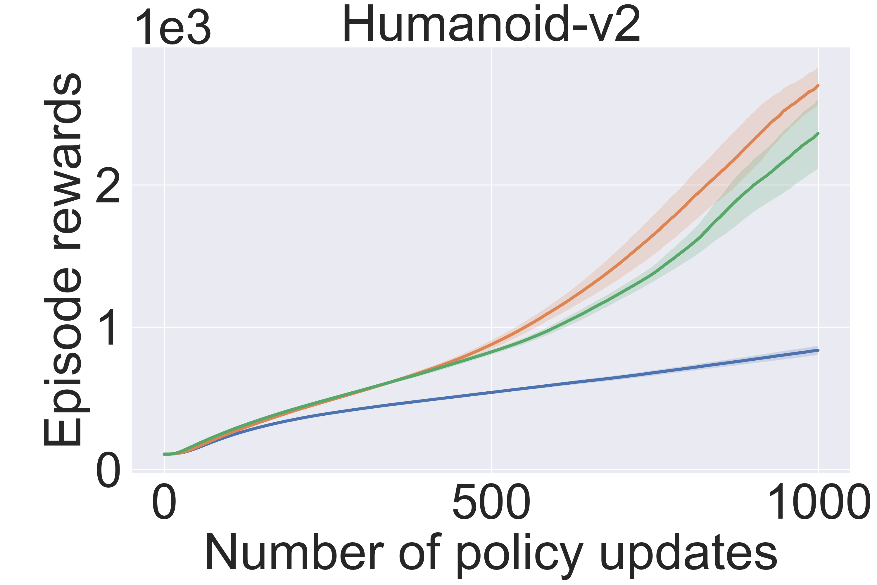
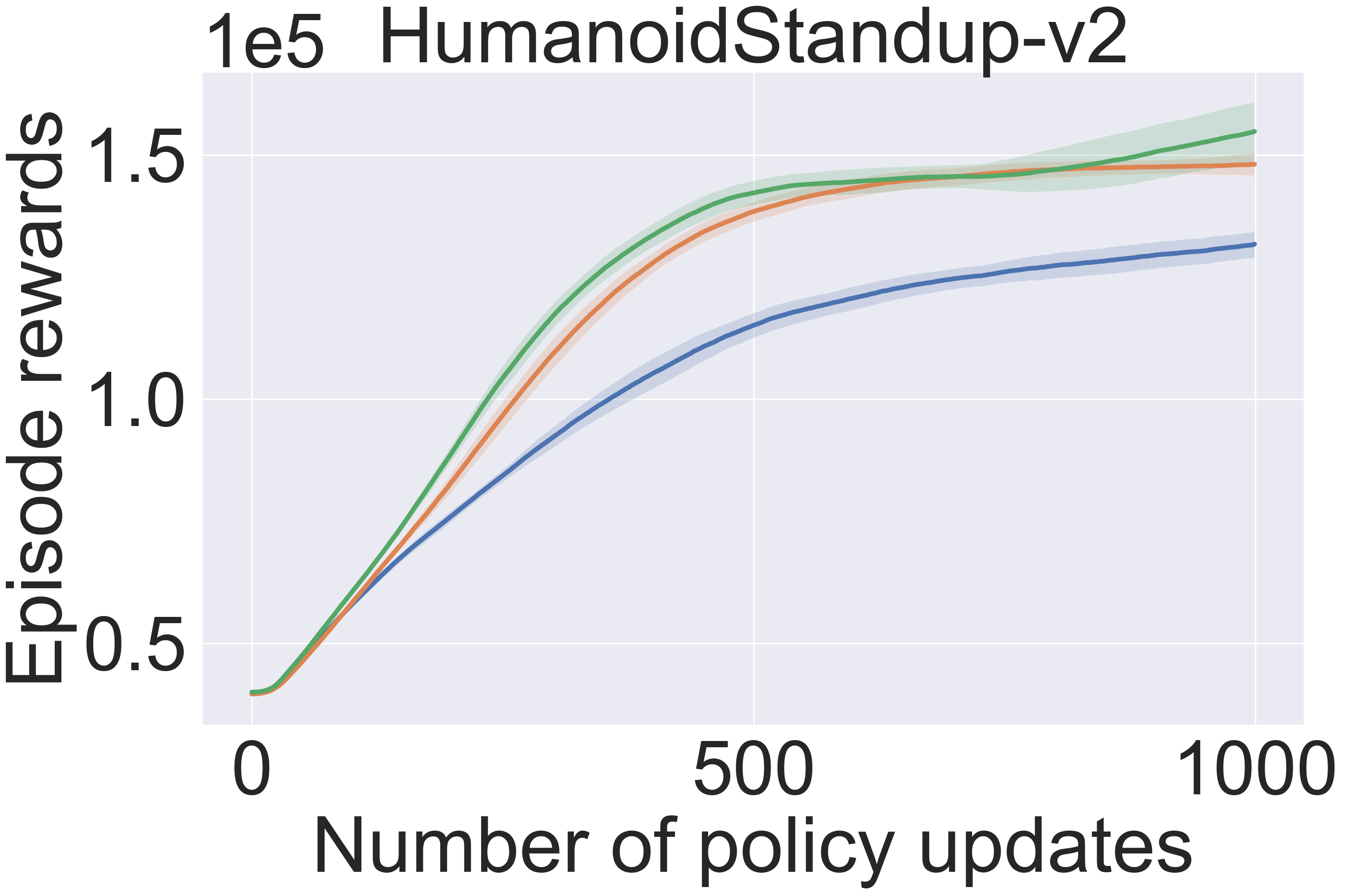
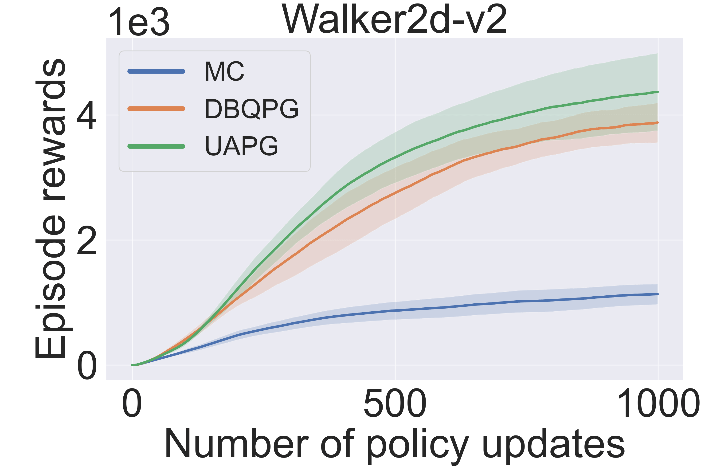
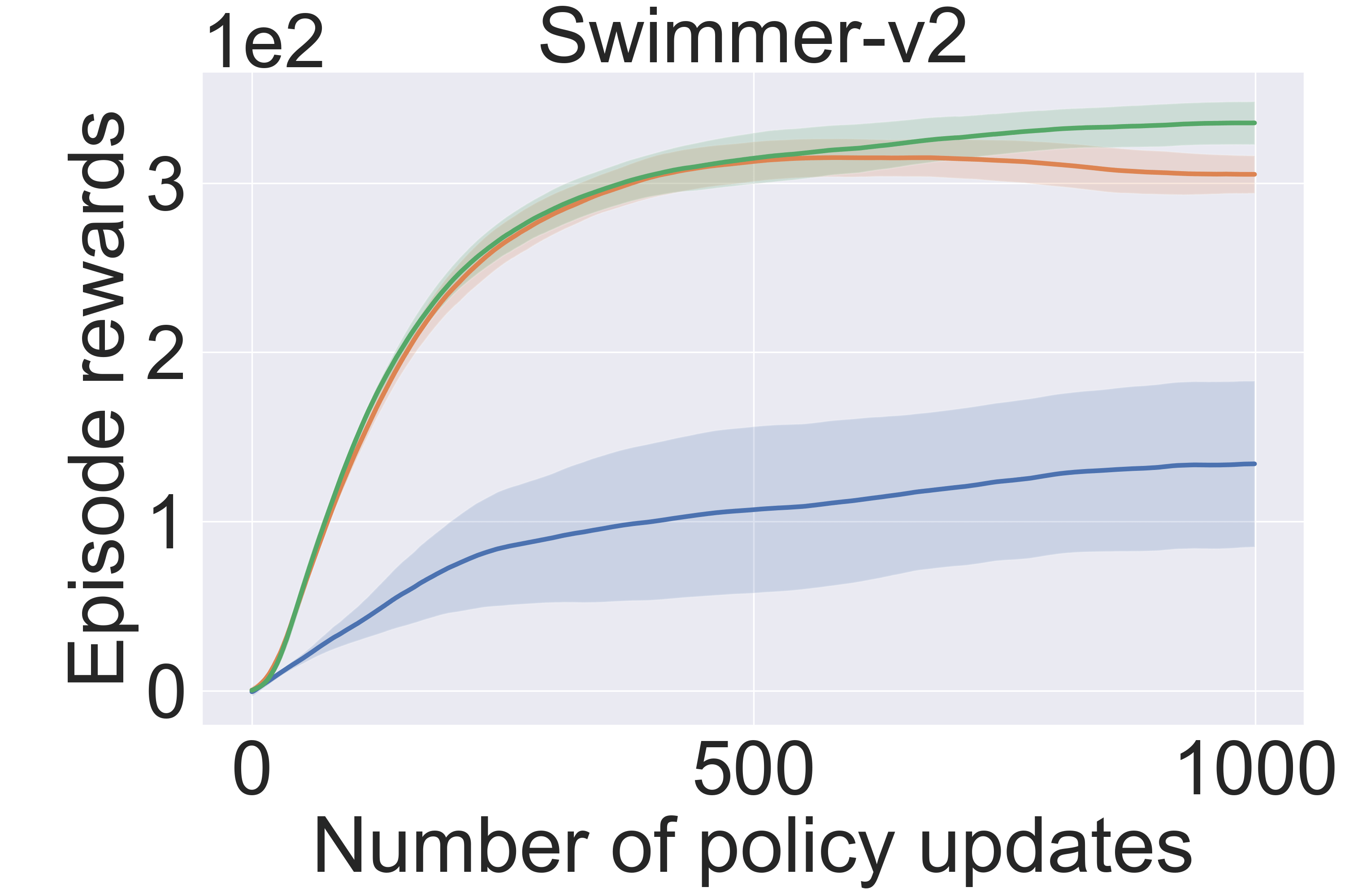
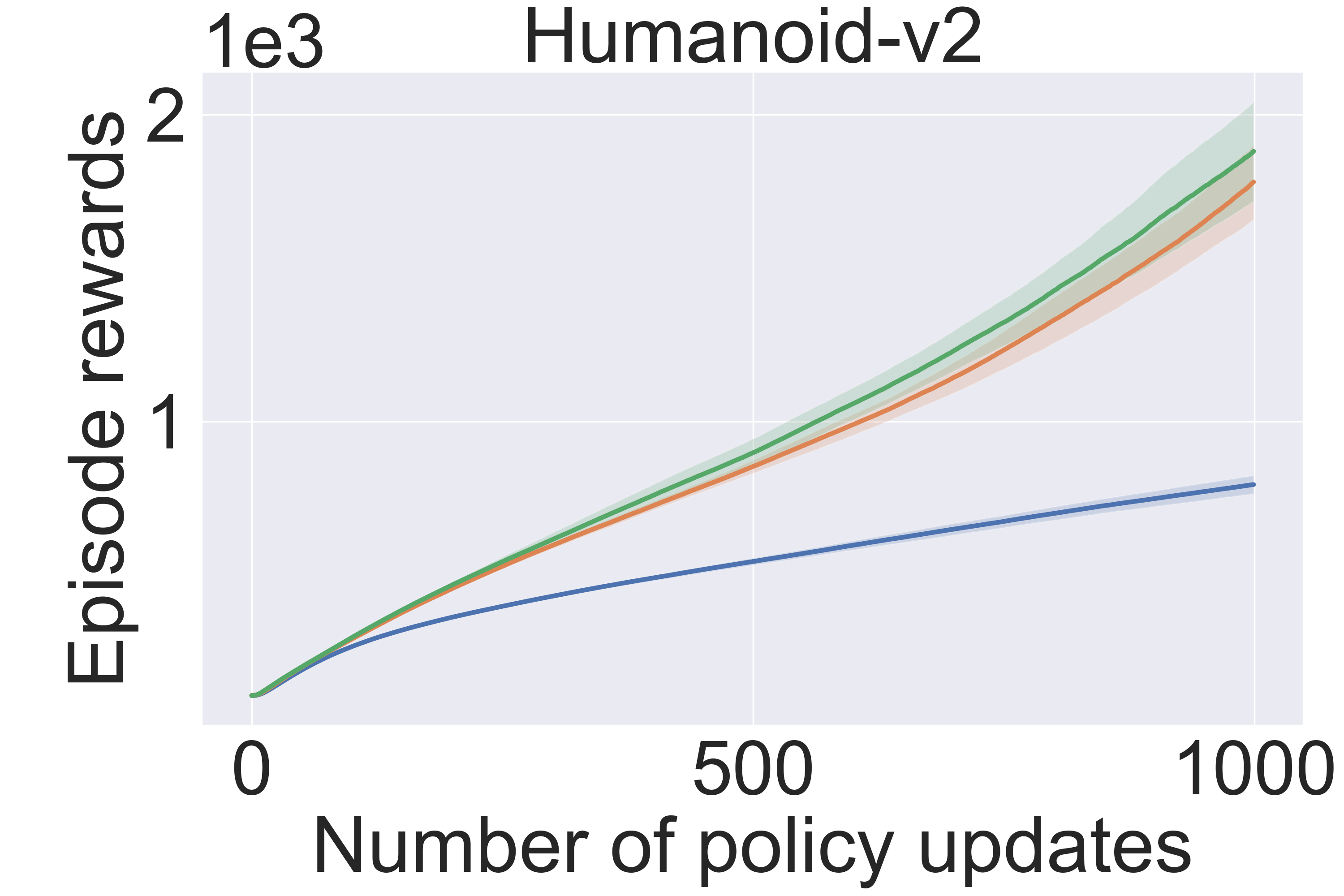
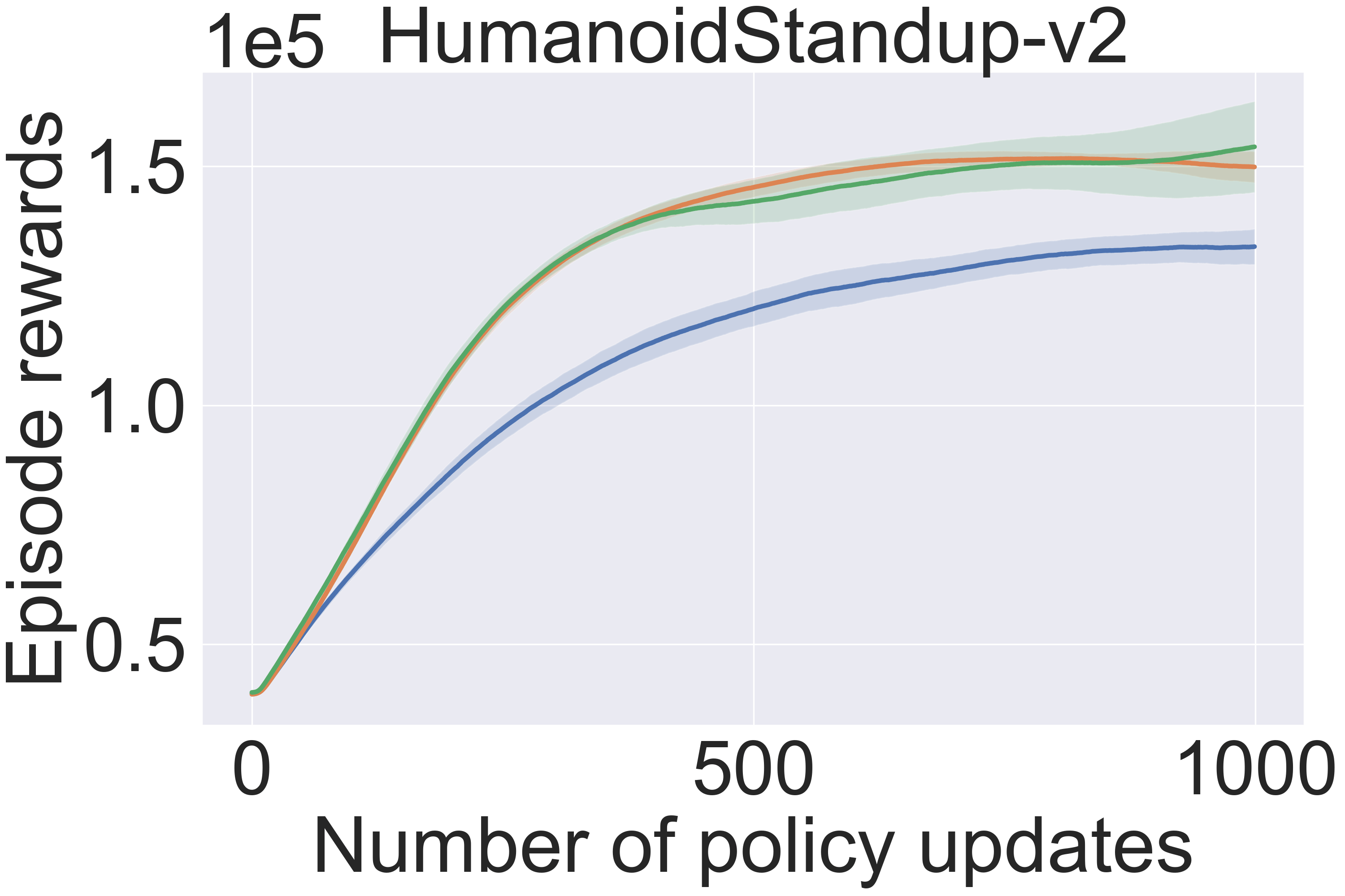
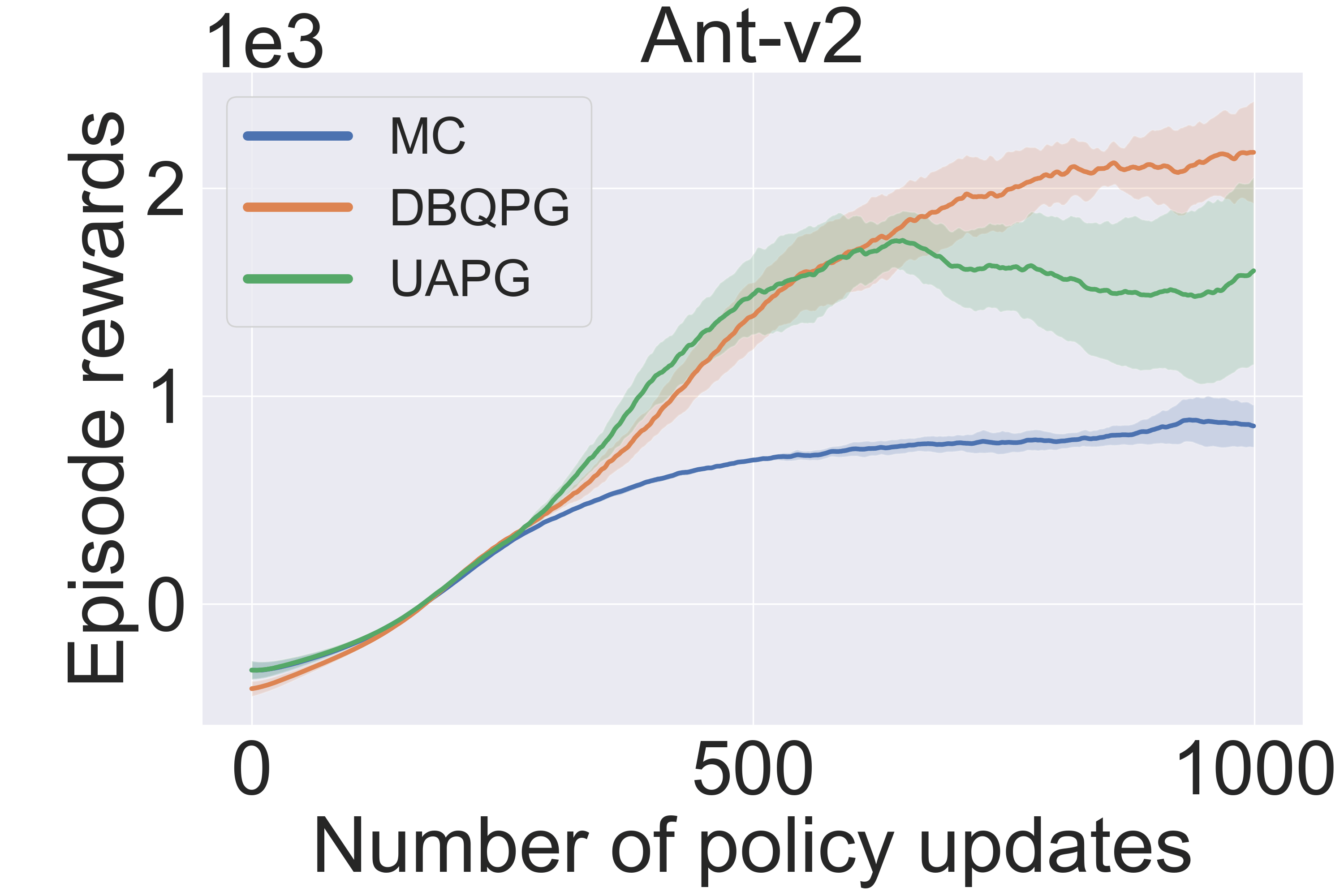
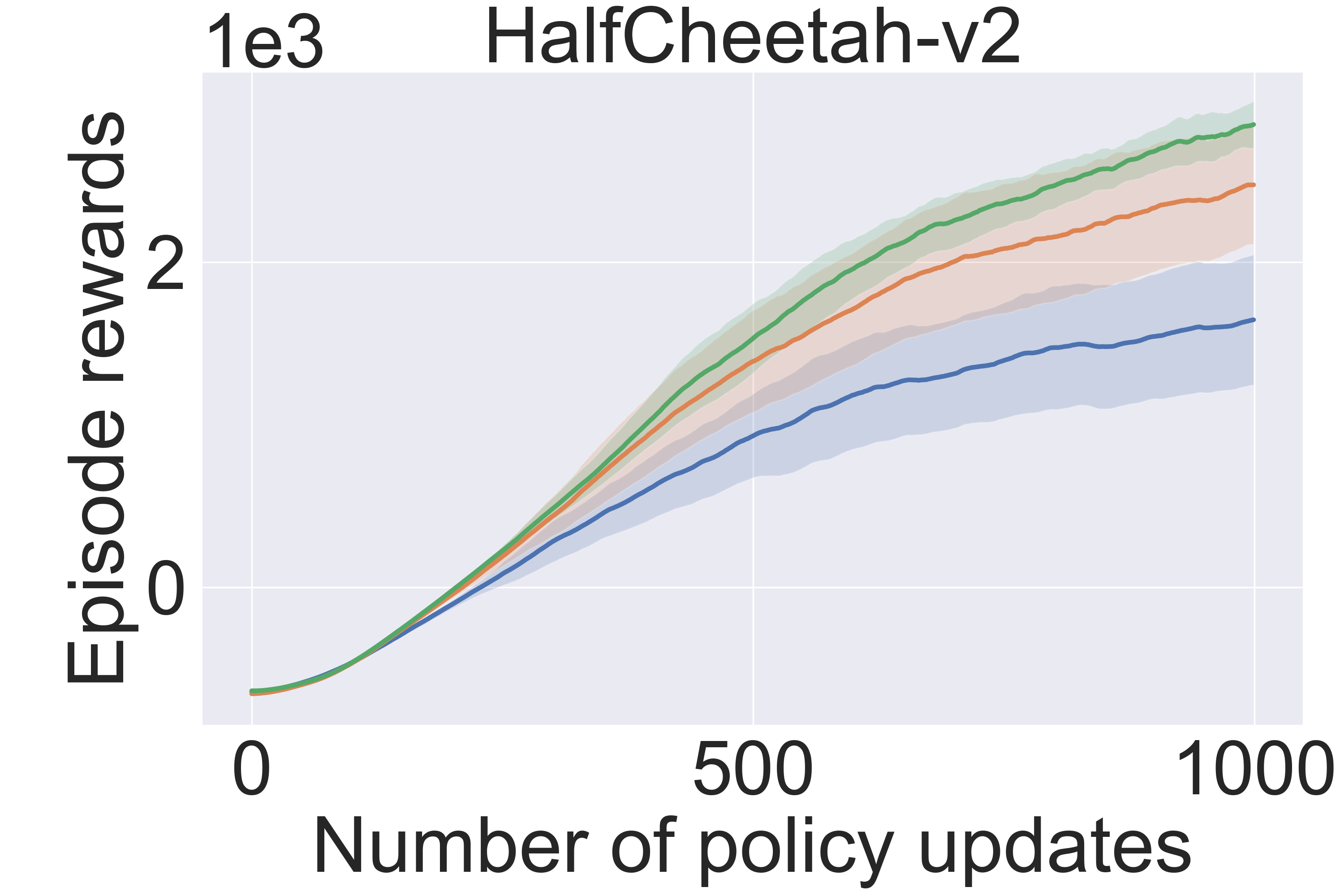
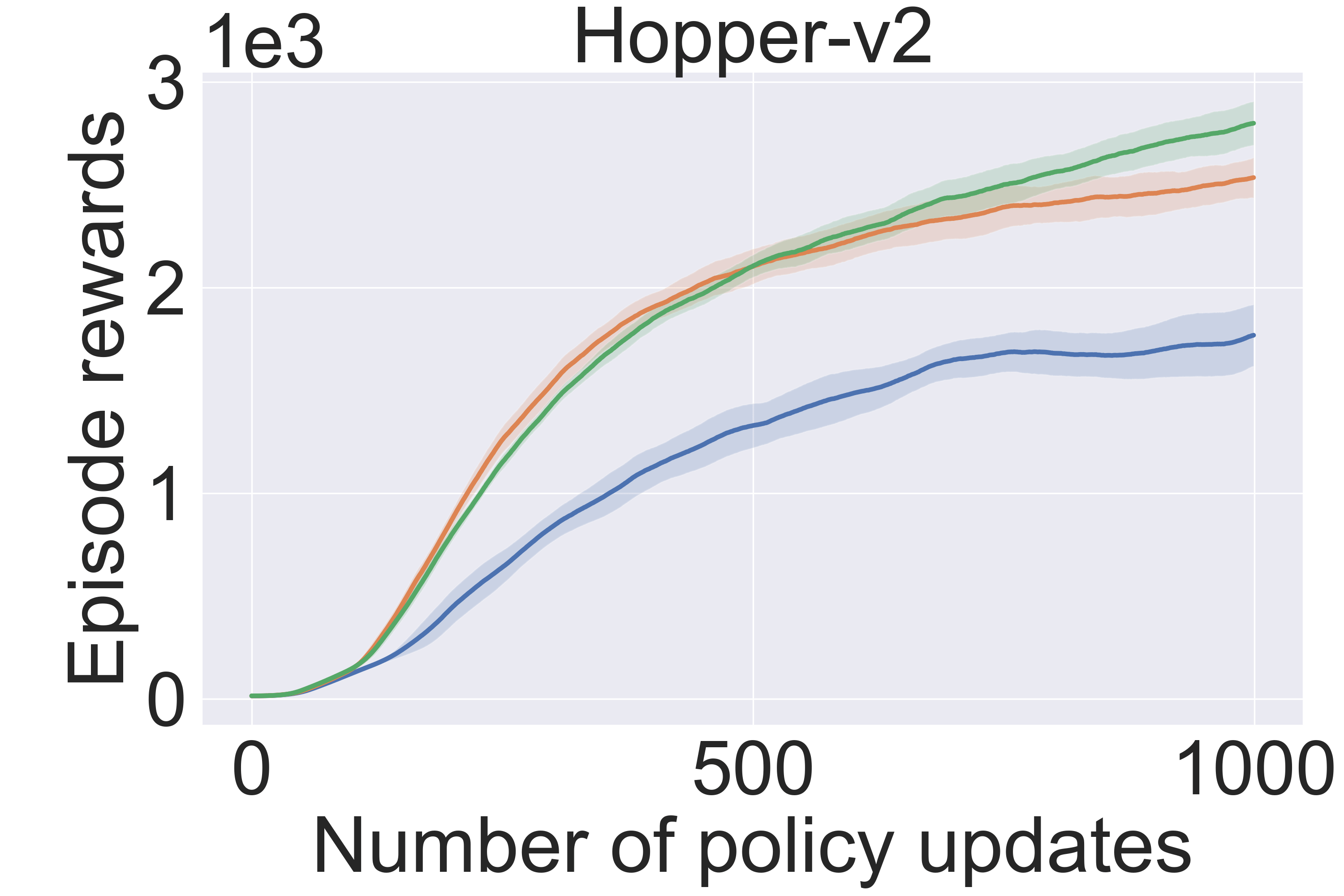
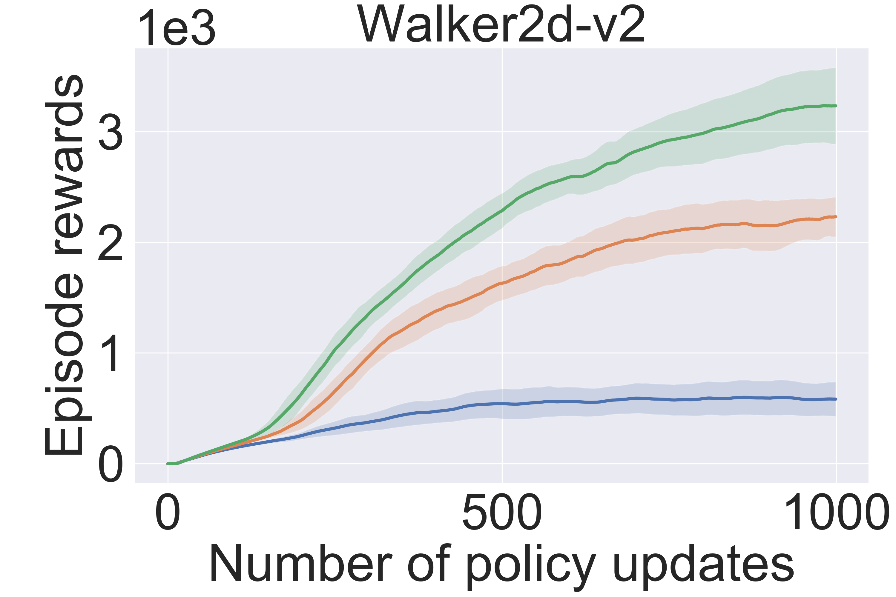
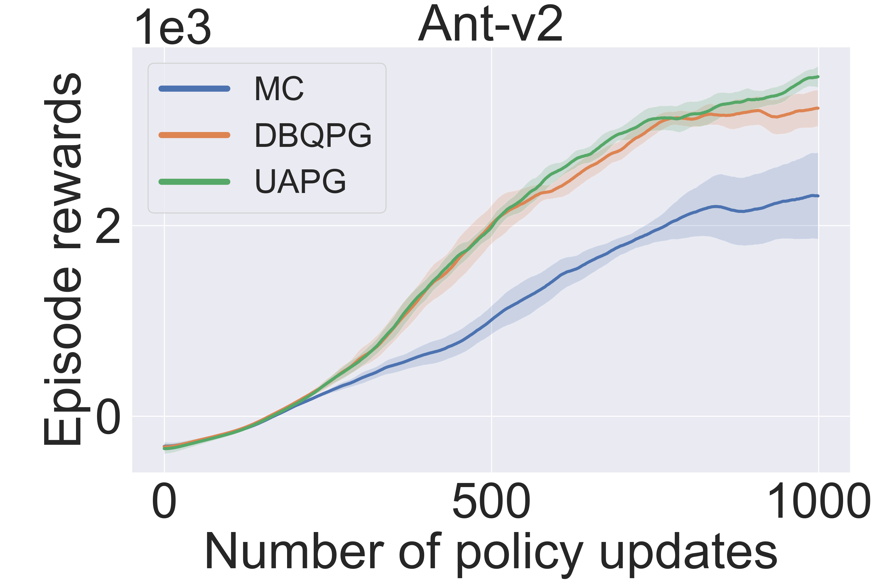
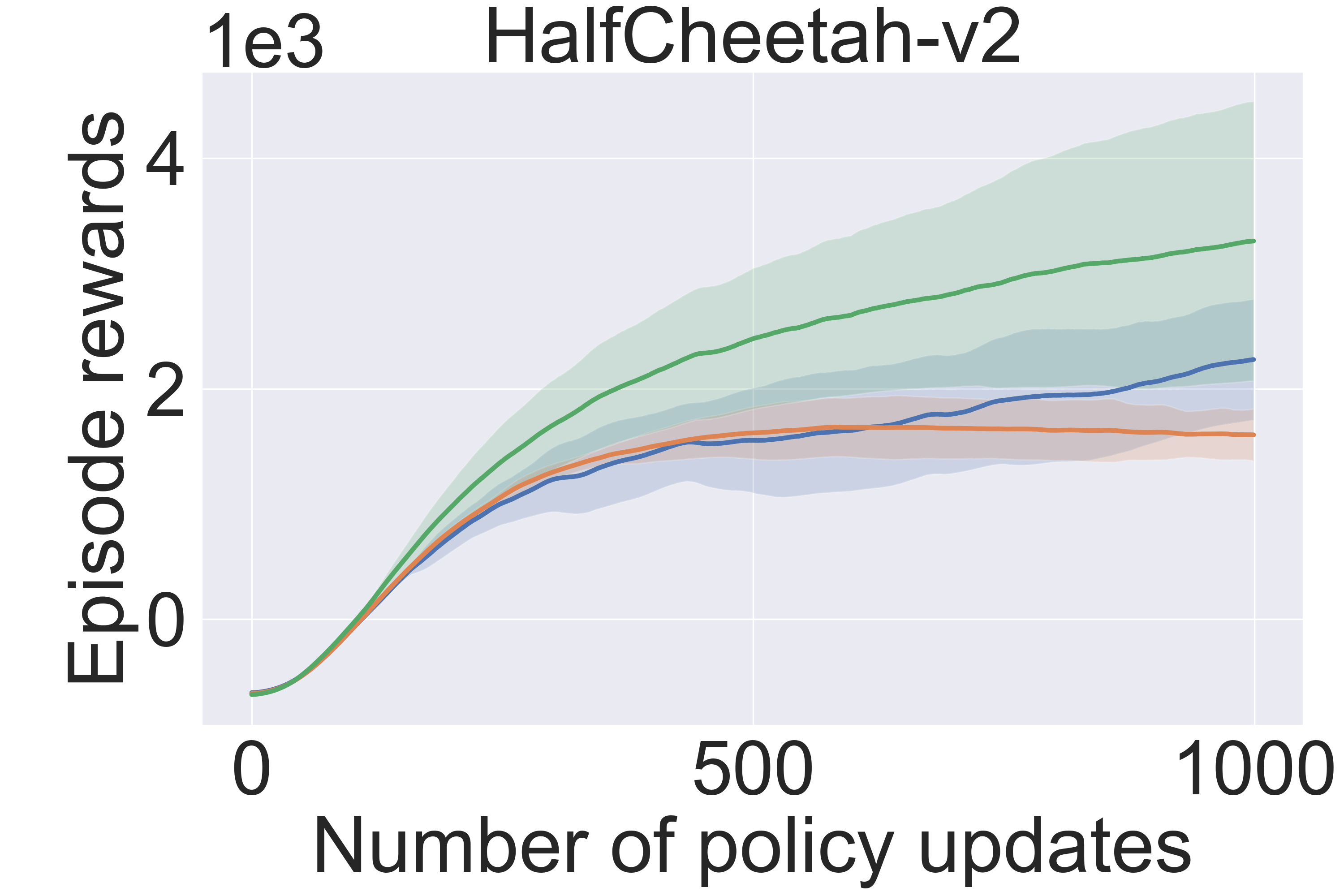
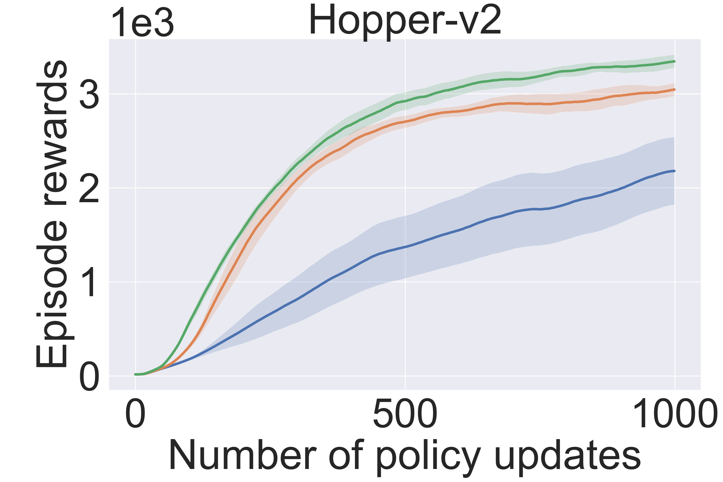
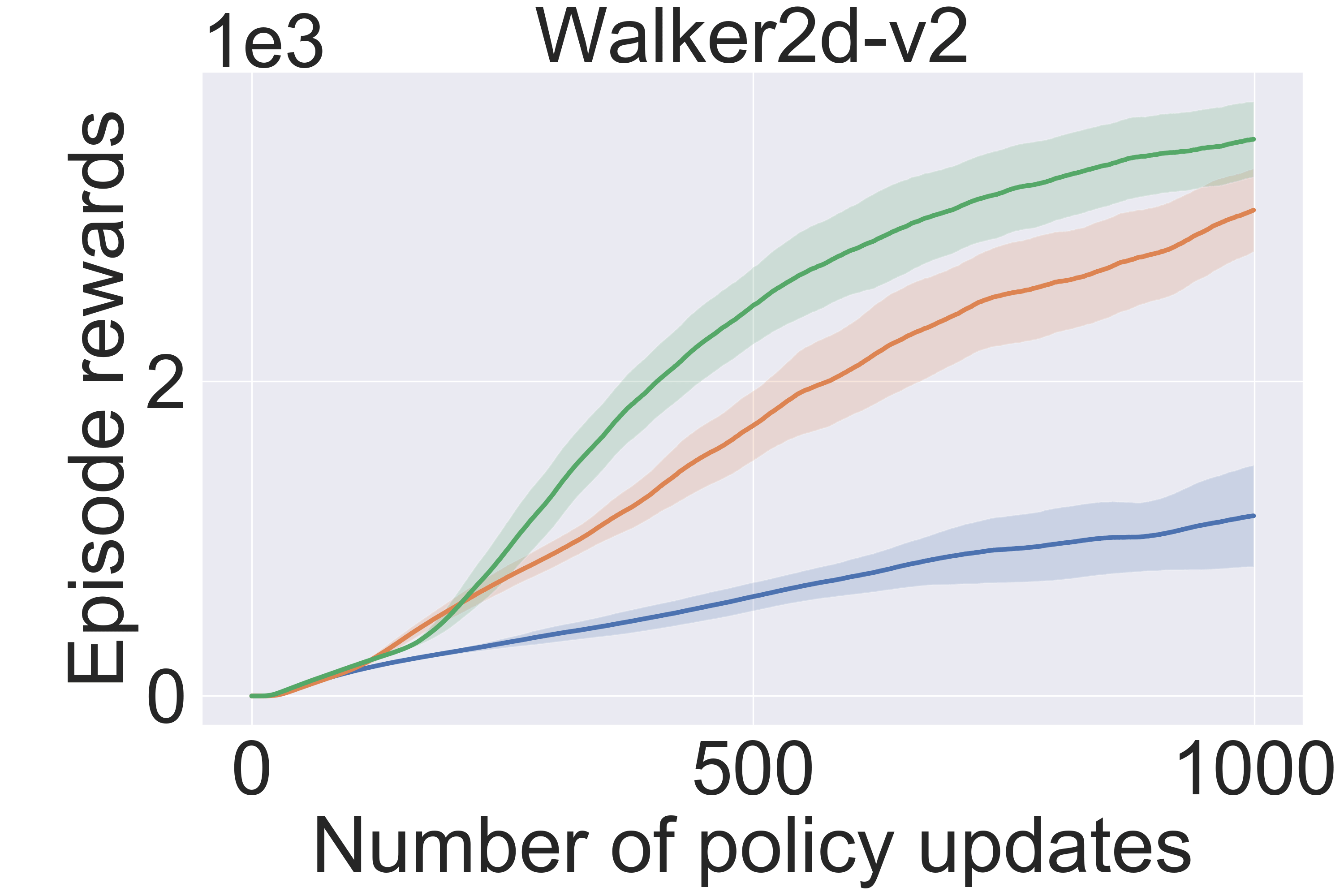
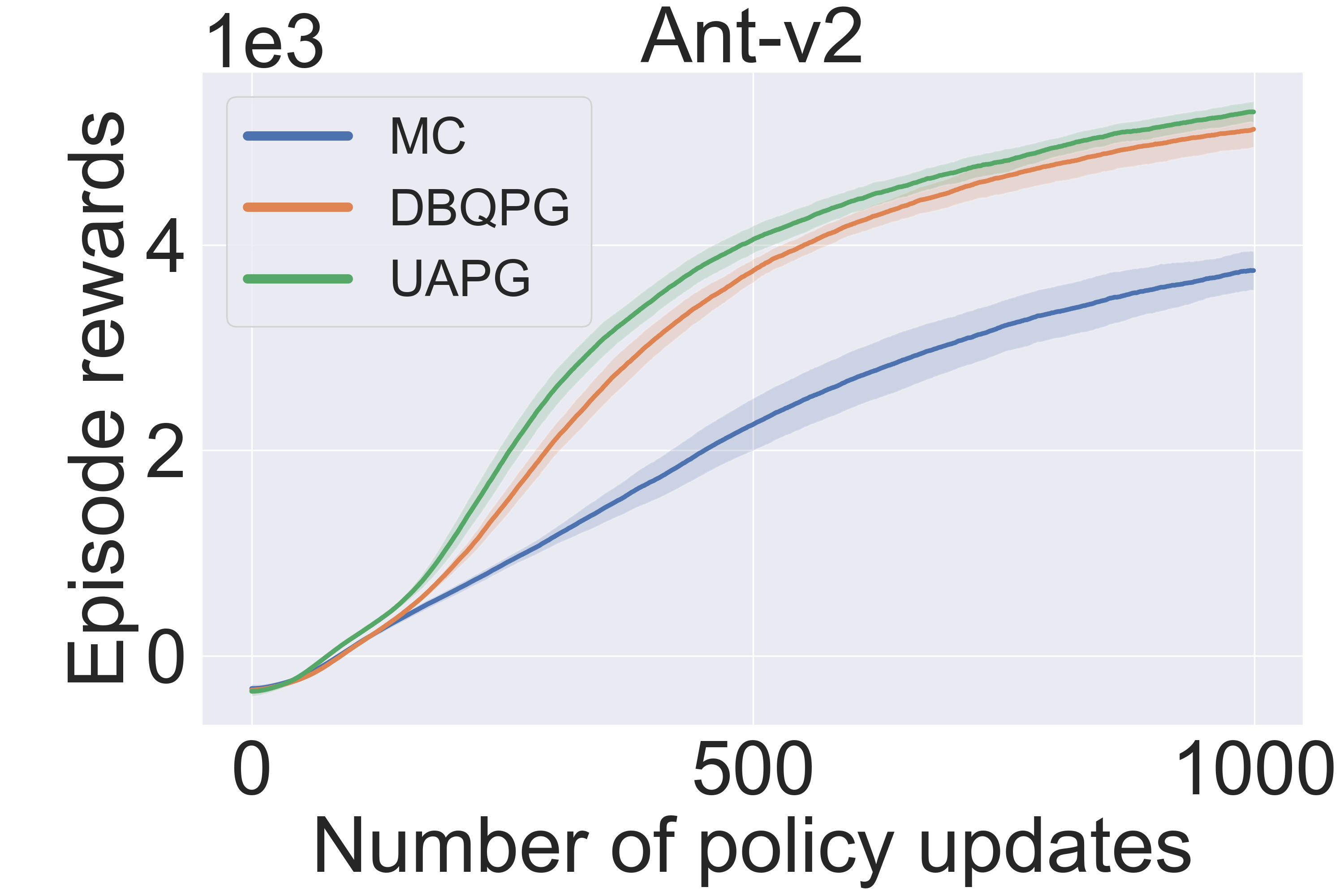
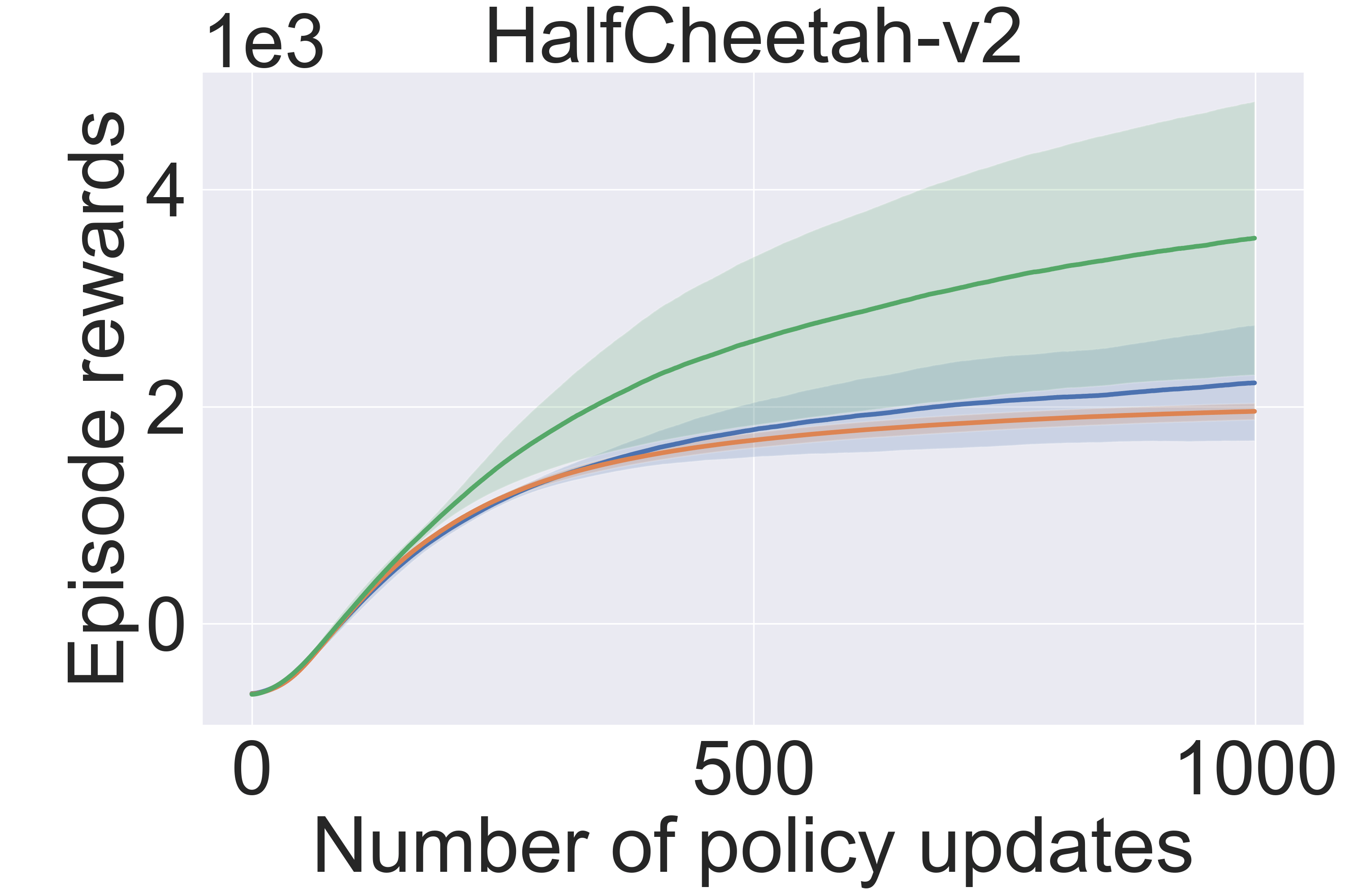
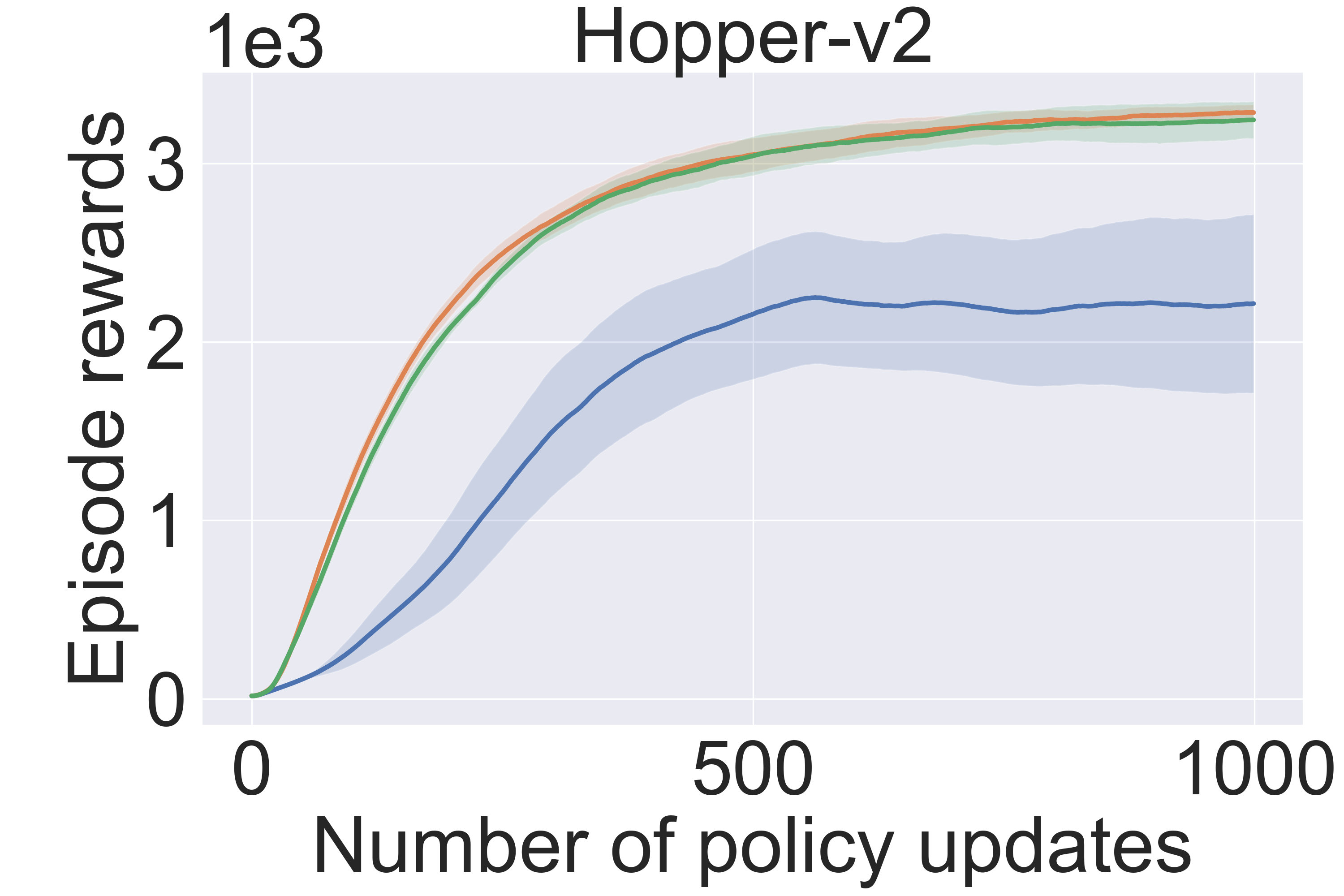
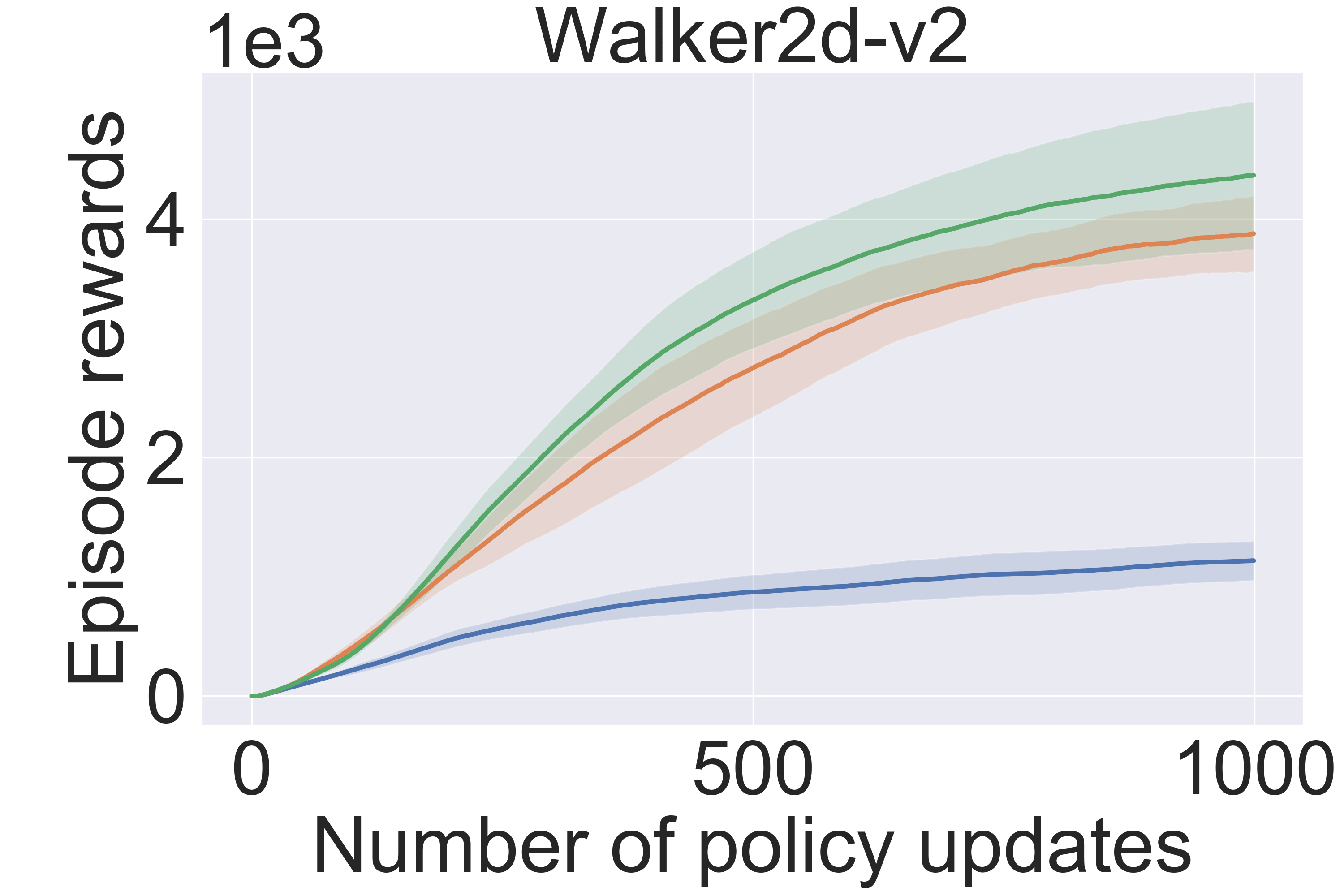
Compatibility with Deep PG Algorithms: We examine the compatibility of BQ-based methods with the following on-policy deep policy gradient algorithms: (i) Vanilla policy gradient, (ii) natural policy gradient (NPG), and (iii) trust region policy optimization (TRPO), as shown in Fig. 3. In these experiments, only the MC estimation subroutine is replaced with BQ-based methods, keeping the rest of the algorithm unchanged. Note that for TRPO, we use the UAPG update of NPG to compute the step direction. We observe that DBQPG consistently outperforms MC estimation, both in final performance and sample complexity across all the deep PG algorithms. This observation resonates with our previous finding of the superior gradient quality of DBQPG estimates, and strongly advocates the use of DBQPG over MC for PG estimation.

For UAPG, we observe a similar trend as DBQPG. The advantage of UAPG estimates is more pronounced in the vanilla PG, and NPG experiments since the performance on these algorithms is highly sensitive to the choice of learning rates. UAPG adjusts the stepsize of each gradient component based on its uncertainty, resulting in a robust update in the face of uncertainty, a better sample complexity, and average return. We observe that UAPG performs at least as good as, if not considerably better than, DBQPG on most experiments. Since TRPO updates are less sensitive to the learning rate, UAPG adjustment does not provide a significant improvement over DBQPG.

7 Related Work

The high sample complexity of MC methods has been a long-standing problem in the PG literature (Rubinstein 1969). Previous approaches that address this issue broadly focus on two aspects: (i) improving the quality of PG estimation using a value function approximation (Konda and Tsitsiklis 2003), or (ii) attaining faster convergence by robustly taking larger steps in the right direction. The former class of approaches trade a tolerable level of bias for designing a lower variance PG estimator (Schulman et al. 2016; Reisinger, Stone, and Miikkulainen 2008). Following the latter research direction, Kakade (2001) and Kakade and Langford (2002) suggest replacing the vanilla PG with natural policy gradient (NPG), the steepest descent direction in the policy distribution space. While NPG improves over vanilla PG methods in terms of sample complexity (Peters and Schaal 2008; Agarwal et al. 2019), it is just as vulnerable to catastrophic policy updates. Trust region policy optimization (TRPO) (Schulman et al. 2015) extends the NPG algorithm with a robust stepsize selection mechanism that guarantees monotonic improvements for expected (true) policy updates. However, the practical TRPO algorithm loses its improvement guarantees for stochastic PG estimates, thereby necessitating a large sample size for computing reliable policy updates. The advantages of these approaches, in terms of sample efficiency, are orthogonal to the benefits of DBQPG and UAPG methods.

Another line of research focuses on using Gaussian processes (GP) to directly approximate the PG integral (Ghavamzadeh and Engel 2006). This work was followed by the Bayesian Actor-Critic (BAC) algorithm (Ghavamzadeh and Engel 2007), which exploits the MDP framework for improving the statistical efficiency of PG estimation. Like DBQPG, BAC is a BQ-based PG method that uses a GP to approximate the action-value function. However, BAC is an online algorithm that uses Gaussian process temporal difference (GPTD) (Engel, Mannor, and Meir 2005), a sequential kernel sparsification method, for learning the value function. BAC’s sequential nature and a prohibitive $\mathcal{O}(m^{2}n+m^{3})$ time and $\mathcal{O}(mn+m^{2})$ storage complexity ($m$ is the dictionary size, i.e., the number of inducing points) prevents if from scaling to large non-linear policies and high-dimensional continuous domains. Further, a recent extension of BAC (Ghavamzadeh, Engel, and Valko 2016) uses the uncertainty to adjust the learning rate of policy parameters, $({\bm{I}}-\frac{1}{\nu}{\bm{C}}_{{\bm{\theta}}}^{BQ}){\bm{L}}_{{\bm{\theta}}}^{BQ}$ ($\nu$ is an upper bound for ${\bm{C}}_{{\bm{\theta}}}^{BQ}$), much like the UAPG method. While this update reduces the step-size of more uncertain directions, it does not provide gradient estimates with uniform uncertainty, making it less robust to bad policy updates relative to UAPG. Moreover, this method would not work for NPG and TRPO algorithms as their covariance is the inverse of an ill-conditioned matrix. Refer supplement Sec. G for a more detailed comparison of DBQPG and UAPG with prior BQ-PG works.

8 Discussion

We study the problem of estimating accurate policy gradient (PG) estimates from a finite number of samples. This problem becomes relevant in numerous RL applications where an agent needs to estimate the PG using samples gathered through interaction with the environment. Monte-Carlo (MC) methods are widely used for PG estimation despite offering high-variance gradient estimates and a slow convergence rate. We propose DBQPG, a high-dimensional generalization of Bayesian quadrature that, like MC method, estimates PG in linear-time. We empirically study DBQPG and demonstrate its effectiveness over MC methods. We show that DBQPG provides more accurate gradient estimates, along with a significantly smaller variance in the gradient estimation. Next, we show that replacing the MC method with DBQPG in the gradient estimation subroutine of three deep PG algorithms, viz., Vanilla PG, NPG, and TRPO, offers consistent gains in sample complexity and average return. These results strongly recommend the substitution of MC estimator with DBQPG in deep PG algorithms.

To obtain reliable policy updates from stochastic gradient estimates, one needs to estimate the uncertainty in gradient estimation, in addition to the gradient estimation itself. The proposed DBQPG method additionally provides this uncertainty along with the PG estimate. We propose UAPG, a PG method that uses DBQPG’s uncertainty to normalize the gradient components by their uncertainties, returning a uniformly uncertain gradient estimate. Such a normalization will lower the step size of gradient components with high uncertainties, resulting in reliable updates with robust step sizes. We show that UAPG further improves the sample complexity over DBQPG on Vanilla PG, NPG, and TRPO algorithms. Overall, our study shows that it is possible to scale Bayesian quadrature to high-dimensional settings, while its better gradient estimation and well-calibrated gradient uncertainty can significantly boost the performance of deep PG algorithms.

Ethics Statement

When deploying deep policy gradient (PG) algorithms for learning control policies in physical systems, sample efficiency becomes an important design criteria. In the past, numerous works have focused on improving the sample efficiency of PG estimation through variance reduction, robust stepsize selection, etc. In this paper, we propose deep Bayesian quadrature policy gradient (DBQPG), a statistically efficient policy gradient estimator that offers orthogonal benefits for improving the sample efficiency. In comparison to Monte-Carlo estimation, the default choice for PG estimation, DBQPG returns more accurate gradient estimates with much lower empirical variance. Since DBQPG is a general gradient estimation subroutine, it can directly replace Monte-Carlo estimation in most policy gradient algorithms, as already demonstrated in our paper. Therefore, we think that the DBQPG method directly benefits most policy gradient algorithms and is indirectly beneficial for several downstream reinforcement learning applications.

We also propose uncertainty aware policy gradient (UAPG), a principled approach for incorporating the uncertainty in gradient estimation (also quantified by the DBQPG method) to obtain reliable PG estimates. UAPG lowers the risk of catastrophic performance degradation with stochastic policy updates, and empirically performs at least as good as, if not better than, the DBQPG method. Hence, we believe that the UAPG method is more relevant to reinforcement learning applications with safety considerations, such as robotics.

Appendix A Useful Identities

Expectation of the score vector ${\bm{u}}(z)=\nabla_{{\bm{\theta}}}\log\pi_{{\bm{\theta}}}(a|s)$ under the policy distribution $\pi_{{\bm{\theta}}}(a|s)$ is $\mathbf{0}$:

$$\begin{split}\mathbb{E}_{a\sim\pi_{\bm{\theta}}(.|s)}\left[{\bm{u}}(z)\right]&=\mathbb{E}_{a\sim\pi_{{\bm{\theta}}}(.|s)}\left[\nabla_{{\bm{\theta}}}\log\pi_{{\bm{\theta}}}(a|s)\right]=\int\pi_{{\bm{\theta}}}(a|s)\nabla_{{\bm{\theta}}}\log\pi_{{\bm{\theta}}}(a|s)da\\ &=\int\pi_{{\bm{\theta}}}(a|s)\frac{\nabla_{{\bm{\theta}}}\pi_{{\bm{\theta}}}(a|s)}{\pi_{{\bm{\theta}}}(a|s)}da=\int\nabla_{{\bm{\theta}}}\pi_{{\bm{\theta}}}(a|s)da\\ &=\nabla_{{\bm{\theta}}}\left(\int\pi_{{\bm{\theta}}}(a|s)da\right)=\nabla_{{\bm{\theta}}}(1)=\mathbf{0}\end{split}$$ (13)

From Eq. 13, the expectation of the Fisher kernel $k_{f}$ under the policy distribution $\pi_{{\bm{\theta}}}(a|s)$ is also $0$:

$$\begin{split}\mathbb{E}_{a\sim\pi_{\bm{\theta}}(.|s)}\left[k_{f}(z,z^{\prime})\right]&=\mathbb{E}_{a\sim\pi_{\bm{\theta}}(.|s)}\left[{\bm{u}}(z)^{\top}{\bm{G}}^{-1}{\bm{u}}(z^{\prime})\right]=\mathbb{E}_{a\sim\pi_{\bm{\theta}}(.|s)}\left[{\bm{u}}(z)^{\top}\right]{\bm{G}}^{-1}{\bm{u}}(z^{\prime})=0\end{split}$$ (14)

Appendix B Bayesian Quadrature for Estimating Policy Gradient Integral

Bayesian quadrature (BQ) (O’Hagan 1991) provides the required machinery for estimating the numerical integration in PG (Eq. 2), by using a Gaussian process (GP) function approximation for the action-value function $Q_{\pi_{\bm{\theta}}}$. More specifically, we choose a zero mean GP, i.e., $\mathbb{E}\left[Q_{\pi_{\bm{\theta}}}(z)\right]=0$, with a prior covariance function $k(z_{p},z_{q})=\mathrm{Cov}[Q_{\pi_{\bm{\theta}}}(z_{p}),Q_{\pi_{\bm{\theta}}}(z_{q})]$ and an additive Gaussian noise with variance $\sigma^{2}$. One benefit of this prior is that the joint distribution over any finite number of action-values (indexed by the state-action inputs, $z\in\mathcal{Z}$) is also Gaussian:

$$\begin{split}{\bm{Q}}_{\pi_{\bm{\theta}}}&=[Q_{\pi_{\bm{\theta}}}(z_{1}),...,Q_{\pi_{\bm{\theta}}}(z_{n})]\sim\mathcal{N}(0,{\bm{K}}),\end{split}$$ (15)

where ${\bm{K}}$ is the Gram matrix with entries ${\bm{K}}_{p,q}=k(z_{p},z_{q})$. This GP prior is conditioned on the observed samples $\mathcal{D}=\{z_{i}\}_{i=1}^{n}$ drawn from $\rho^{\pi_{\theta}}$ to obtain the posterior moments of $Q_{\pi_{\bm{\theta}}}$:

$$\begin{split}\mathbb{E}\left[Q_{\pi_{\bm{\theta}}}(z)|\mathcal{D}\right]&={\bm{k}}(z)^{\top}({\bm{K}}+\sigma^{2}{\bm{I}})^{-1}{\bm{Q}},\\ \mathrm{Cov}\left[Q_{\pi_{\bm{\theta}}}(z_{1}),Q_{\pi_{\bm{\theta}}}(z_{2})|\mathcal{D}\right]&=k(z_{1},z_{2})-{\bm{k}}(z_{1})^{\top}({\bm{K}}+\sigma^{2}{\bm{I}})^{-1}{\bm{k}}(z_{2}),\\ \text{where }{\bm{k}}(z)=[k(z_{1},z&),...,k(z_{n},z)],\;{\bm{K}}=[{\bm{k}}(z_{1}),...,{\bm{k}}(z_{n})].\end{split}$$ (16)

Since the transformation from $Q_{\pi_{\bm{\theta}}}(z)$ to $\nabla_{{\bm{\theta}}}J({\bm{\theta}})$ happens through a linear integral operator (Eq. 2), the posterior moments of $Q_{\pi_{\bm{\theta}}}$ can be used to compute a Gaussian approximation of $\nabla_{{\bm{\theta}}}J({\bm{\theta}})$:

$$\quad\qquad\displaystyle{\bm{L}}_{{\bm{\theta}}}^{BQ}=\mathbb{E}\left[\nabla_{{\bm{\theta}}}J({\bm{\theta}})|\mathcal{D}\right]=\displaystyle\int\rho^{\pi_{\bm{\theta}}}(z){\bm{u}}(z)\mathbb{E}\left[Q_{\pi_{\bm{\theta}}}(z)|\mathcal{D}\right]dz$$

$$\quad\qquad\qquad=\displaystyle\left(\int\rho^{\pi_{\bm{\theta}}}(z){\bm{u}}(z){\bm{k}}(z)^{\top}dz\right)({\bm{K}}+\sigma^{2}{\bm{I}})^{-1}{\bm{Q}}$$ (17)

$$\displaystyle{\bm{C}}_{{\bm{\theta}}}^{BQ} =\mathrm{Cov}[\nabla_{{\bm{\theta}}}J({\bm{\theta}})|\mathcal{D}]=\displaystyle\int\rho^{\pi_{\bm{\theta}}}(z_{1})\rho^{\pi_{\bm{\theta}}}(z_{2}){\bm{u}}(z_{1})\mathrm{Cov}[Q_{\pi_{\bm{\theta}}}(z_{1}),Q_{\pi_{\bm{\theta}}}(z_{2})|\mathcal{D}]{\bm{u}}(z_{2})^{\top}dz_{1}dz_{2},$$

$$=\displaystyle\int\rho^{\pi_{\bm{\theta}}}(z_{1})\rho^{\pi_{\bm{\theta}}}(z_{2}){\bm{u}}(z_{1})\Big{(}k(z_{1},z_{2})-{\bm{k}}(z_{1})^{\top}({\bm{K}}+\sigma^{2}{\bm{I}})^{-1}{\bm{k}}(z_{2})\Big{)}{\bm{u}}(z_{2})^{\top}dz_{1}dz_{2},$$

where the posterior mean ${\bm{L}}_{{\bm{\theta}}}^{BQ}$ can be interpreted as the PG estimate and the posterior covariance ${\bm{C}}_{{\bm{\theta}}}^{BQ}$ quantifies the uncertainty in the PG estimate. However, the integrals in Eq. B cannot be solved analytically for an arbitrary GP prior covariance function $k(z_{1},z_{2})$. Ghavamzadeh and Engel (2007) showed that these integrals have analytical solutions when the GP kernel $k$ is the additive composition of an arbitrary state kernel $k_{s}$ and the (indispensable) Fisher kernel $k_{f}$:

$$k(z_{1},z_{2})=c_{1}k_{s}(s_{1},s_{2})+c_{2}k_{f}(z_{1},z_{2}),\quad k_{f}(z_{1},z_{2}) ={\bm{u}}(z_{1})^{\top}{\bm{G}}^{-1}{\bm{u}}(z_{2}),$$ (18)

where $c_{1},c_{2}$ are hyperparameters and ${\bm{G}}$ is the Fisher information matrix of the policy $\pi_{\bm{\theta}}$. Using the following definitions,

$${\bm{k}}_{f}(z)={\bm{U}}^{\top}{\bm{G}}^{-1}{\bm{u}}(z),\ \ {\bm{K}}_{f}={\bm{U}}^{\top}{\bm{G}}^{-1}{\bm{U}},\ \ {\bm{K}}=c_{1}{\bm{K}}_{s}+c_{2}{\bm{K}}_{f},\ \ {\bm{G}}=\mathbb{E}_{z\sim\rho^{\pi_{\bm{\theta}}}}[{\bm{u}}(z){\bm{u}}(z)^{\top}]\approx\frac{1}{n}{\bm{U}}{\bm{U}}^{\top},$$ (19)

the closed-form expressions for PG estimate ${\bm{L}}_{{\bm{\theta}}}^{BQ}$ and its uncertainty ${\bm{C}}_{{\bm{\theta}}}^{BQ}$ are obtained as follows,

$$\begin{split}\displaystyle{\bm{L}}_{{\bm{\theta}}}^{BQ}&=\mathbb{E}\left[\nabla_{{\bm{\theta}}}J({\bm{\theta}})|\mathcal{D}\right]=\displaystyle\int\rho^{\pi_{\bm{\theta}}}(z){\bm{u}}(z)\mathbb{E}\left[Q_{\pi_{\bm{\theta}}}(z)|\mathcal{D}\right]dz\\ &=\mathbb{E}_{z\sim\rho^{\pi_{\bm{\theta}}}}\left[{\bm{u}}(z)\mathbb{E}[Q_{\pi_{\bm{\theta}}}(z)|\mathcal{D}]\right]=\mathbb{E}_{z\sim\rho^{\pi_{\bm{\theta}}}}\left[{\bm{u}}(z){\bm{k}}(z)^{\top}\right]({\bm{K}}+\sigma^{2}{\bm{I}})^{-1}{\bm{Q}}\\ &=\left(c_{1}\mathbb{E}_{z\sim\rho^{\pi_{\bm{\theta}}}}\left[{\bm{u}}(z){\bm{k}}_{s}(s)^{\top}\right]+c_{2}\mathbb{E}_{z\sim\rho^{\pi_{\bm{\theta}}}}\left[{\bm{u}}(z){\bm{k}}_{f}(z)^{\top}\right]\right)({\bm{K}}+\sigma^{2}{\bm{I}})^{-1}{\bm{Q}}\\ &\;\;\;\;\;\text{$\mathrel{\text{\char 210\relax}}$ ${\bm{k}}_{s}$ term disappears since the integral of ${\bm{u}}(z)$ over action-dims is 0 from Eq.~{}\ref{eqn:appendix_logprob_expectiation}}\\ &=c_{2}\mathbb{E}_{z\sim\rho^{\pi_{\bm{\theta}}}}\left[{\bm{u}}(z){\bm{k}}_{f}(z)^{\top}\right]({\bm{K}}+\sigma^{2}{\bm{I}})^{-1}{\bm{Q}}\\ &=c_{2}\mathbb{E}_{z\sim\rho^{\pi_{\bm{\theta}}}}\left[{\bm{u}}(z){\bm{u}}(z)^{\top}\right]{\bm{G}}^{-1}{\bm{U}}({\bm{K}}+\sigma^{2}{\bm{I}})^{-1}{\bm{Q}}\quad\text{$\mathrel{\text{\char 210\relax}}$ from ${\bm{k}}_{f}$ definition in Eq.~{}\ref{eqn:appendix_kernel_equations}}\\ &=c_{2}{\bm{G}}\>{\bm{G}}^{-1}{\bm{U}}(c_{1}{\bm{K}}_{s}+c_{2}{\bm{K}}_{f}+\sigma^{2}{\bm{I}})^{-1}{\bm{Q}}\qquad\qquad\text{$\mathrel{\text{\char 210\relax}}$ from ${\bm{G}}$ \;definition in Eq.~{}\ref{eqn:appendix_kernel_equations}}\\ &=c_{2}{\bm{U}}(c_{1}{\bm{K}}_{s}+c_{2}{\bm{K}}_{f}+\sigma^{2}{\bm{I}})^{-1}{\bm{Q}}\end{split}$$ (20)

$$\begin{split}\displaystyle{\bm{C}}_{{\bm{\theta}}}^{BQ}&=\mathrm{Cov}\left[\nabla_{{\bm{\theta}}}J({\bm{\theta}})|\mathcal{D}\right]=\displaystyle\int dz_{1}dz_{2}\rho^{\pi_{\bm{\theta}}}(z_{1})\rho^{\pi_{\bm{\theta}}}(z_{2}){\bm{u}}(z_{1})\mathrm{Cov}\left[Q_{\pi_{\bm{\theta}}}(z_{1}),Q_{\pi_{\bm{\theta}}}(z_{2})|\mathcal{D}\right]{\bm{u}}(z_{2})^{\top}\\ &=\mathbb{E}_{z_{1},z_{2}\sim\rho^{\pi_{\bm{\theta}}}}\left[{\bm{u}}(z_{1})\mathrm{Cov}\left[Q_{\pi_{\bm{\theta}}}(z_{1}),Q_{\pi_{\bm{\theta}}}(z_{2})|\mathcal{D}\right]{\bm{u}}(z_{2})^{\top}\right]\\ &=\mathbb{E}_{z_{1},z_{2}\sim\rho^{\pi_{\bm{\theta}}}}\left[{\bm{u}}(z_{1})\Big{(}k(z_{1},z_{2})-{\bm{k}}(z_{1})^{\top}({\bm{K}}+\sigma^{2}{\bm{I}})^{-1}{\bm{k}}(z_{2})\Big{)}{\bm{u}}(z_{2})^{\top}\right]\\ &\qquad\qquad\;\;\;\;\text{$\mathrel{\text{\char 210\relax}}$ $k_{s}$ terms disappear since the integral of ${\bm{u}}(z)$ over action-dims is 0 (Eq.~{}\ref{eqn:appendix_logprob_expectiation})}\\ &=\mathbb{E}_{z_{1},z_{2}\sim\rho^{\pi_{\bm{\theta}}}}\left[{\bm{u}}(z_{1})\Big{(}c_{2}k_{f}(z_{1},z_{2})-c_{2}^{2}{\bm{k}}_{f}(z_{1})^{\top}({\bm{K}}+\sigma^{2}{\bm{I}})^{-1}{\bm{k}}_{f}(z_{2})\Big{)}{\bm{u}}(z_{2})^{\top}\right]\\ &\qquad\qquad\qquad\qquad\qquad\;\text{$\mathrel{\text{\char 210\relax}}$ from the definitions of $k_{f}(z_{1},z_{2})$ (Eq.~{}\ref{eqn:appendix_kernel_definitions}) and ${\bm{k}}_{f}(z)$ (Eq.~{}\ref{eqn:appendix_kernel_equations})}\\ &=\mathbb{E}_{z_{1},z_{2}\sim\rho^{\pi_{\bm{\theta}}}}\left[{\bm{u}}(z_{1}){\bm{u}}(z_{1})^{\top}\Big{(}c_{2}{\bm{G}}^{-1}-c_{2}^{2}{\bm{G}}^{-1}{\bm{U}}({\bm{K}}+\sigma^{2}{\bm{I}})^{-1}{\bm{U}}^{\top}{\bm{G}}^{-1}\Big{)}{\bm{u}}(z_{2}){\bm{u}}(z_{2})^{\top}\right]\\ &=\mathbb{E}_{z_{1}\sim\rho^{\pi_{\bm{\theta}}}}[{\bm{u}}(z_{1}){\bm{u}}(z_{1})^{\top}]\Big{(}c_{2}{\bm{G}}^{-1}-c_{2}^{2}{\bm{G}}^{-1}{\bm{U}}({\bm{K}}+\sigma^{2}{\bm{I}})^{-1}{\bm{U}}^{\top}{\bm{G}}^{-1}\Big{)}\mathbb{E}_{z_{2}\sim\rho^{\pi_{\bm{\theta}}}}[{\bm{u}}(z_{2}){\bm{u}}(z_{2})^{\top}]\\ &={\bm{G}}\Big{(}c_{2}{\bm{G}}^{-1}-c_{2}^{2}{\bm{G}}^{-1}{\bm{U}}({\bm{K}}+\sigma^{2}{\bm{I}})^{-1}{\bm{U}}^{\top}{\bm{G}}^{-1}\Big{)}{\bm{G}}\\ &=c_{2}{\bm{G}}-c_{2}^{2}{\bm{U}}(c_{1}{\bm{K}}_{s}+c_{2}{\bm{K}}_{f}+\sigma^{2}{\bm{I}})^{-1}{\bm{U}}^{\top}\end{split}$$ (21)

Further, the inverse of ${\bm{C}}_{{\bm{\theta}}}^{BQ}$ can also be found analytically using the Woodbury (1950) identity:

$$\begin{split}\displaystyle\left({\bm{C}}_{{\bm{\theta}}}^{BQ}\right)^{-1}&=\left(c_{2}{\bm{G}}-c_{2}^{2}{\bm{U}}(c_{1}{\bm{K}}_{s}+c_{2}{\bm{K}}_{f}+\sigma^{2}{\bm{I}})^{-1}{\bm{U}}^{\top}\right)^{-1}\\ &=\frac{1}{c_{2}}{\bm{G}}^{-1}+{\bm{G}}^{-1}{\bm{U}}\left(c_{1}{\bm{K}}_{s}+c_{2}{\bm{K}}_{f}+\sigma^{2}{\bm{I}}-c_{2}{\bm{U}}^{\top}{\bm{G}}^{-1}{\bm{U}}\right)^{-1}{\bm{U}}^{\top}{\bm{G}}^{-1}\\ &=\frac{1}{c_{2}}{\bm{G}}^{-1}+{\bm{G}}^{-1}{\bm{U}}\left(c_{1}{\bm{K}}_{s}+\sigma^{2}{\bm{I}}\right)^{-1}{\bm{U}}^{\top}{\bm{G}}^{-1}\end{split}$$ (22)

Thus, by choosing the overall kernel as a additive composition of the Fisher kernel $k_{f}$ and an arbitrary state kernel $k_{s}$, the BQ approach has a closed-form expression for the gradient mean ${\bm{L}}_{{\bm{\theta}}}^{BQ}$ and its uncertainty ${\bm{C}}_{{\bm{\theta}}}^{BQ}$ (gradient covariance).

Appendix C More Intuition Behind the GP Kernel Choice

In this section, we analyze the implications of the specified GP kernel choice that provides an analytical solution to the PG integral (shown in the previous section). Particularly, we study the affect of the additive composition of a state kernel $k_{s}$ and the Fisher kernel $k_{f}$ on (i) modeling the $Q_{\pi_{{\bm{\theta}}}}$ function, and consequently (ii) the policy gradient.

C.1 Posterior Moments of the Value Functions

Here, we split $Q_{\pi_{{\bm{\theta}}}}$ function as the sum of a state-value function $V_{\pi_{{\bm{\theta}}}}$ and advantage function $A_{\pi_{{\bm{\theta}}}}$:

$$Q_{\pi_{{\bm{\theta}}}}(z_{t})=V_{\pi_{{\bm{\theta}}}}(s_{t})+A_{\pi_{{\bm{\theta}}}}(z_{t}),\quad V_{\pi_{{\bm{\theta}}}}(s_{t})=\mathbb{E}_{a_{t}\sim\pi_{{\bm{\theta}}}(\cdot|s_{t})}\big{[}Q_{\pi_{{\bm{\theta}}}}(z_{t})\big{]},$$ (23)

where $V_{\pi_{{\bm{\theta}}}}(s)$ is the expected return under $\pi_{{\bm{\theta}}}$ from the initial state $s$, and $A_{\pi_{{\bm{\theta}}}}(z)$ denotes the advantage (or disadvantage) of picking a particular initial action $a$ relative to the policy’s prediction $a\sim\pi_{{\bm{\theta}}}$. The specified GP kernel choice for modeling the $Q_{\pi_{\bm{\theta}}}$ function approximates $V_{\pi_{\bm{\theta}}}$ and $A_{\pi_{\bm{\theta}}}$ as follows:

$$\begin{split}\mathbb{E}\left[V_{\pi_{\bm{\theta}}}(s)|\mathcal{D}\right]&=\mathbb{E}_{a\sim\pi_{\bm{\theta}}(.|s)}\left[\mathbb{E}\left[Q_{\pi_{\bm{\theta}}}(z)|\mathcal{D}\right]\right]=\mathbb{E}_{a\sim\pi_{\bm{\theta}}(.|s)}\left[{\bm{k}}(z)^{\top}\right]({\bm{K}}+\sigma^{2}{\bm{I}})^{-1}{\bm{Q}}\\ &=\mathbb{E}_{a\sim\pi_{\bm{\theta}}(.|s)}\left[\left(c_{1}{\bm{k}}_{s}(s)+c_{2}{\bm{k}}_{f}(z)\right)^{\top}\right]({\bm{K}}+\sigma^{2}{\bm{I}})^{-1}{\bm{Q}}\\ &=\left(c_{1}{\bm{k}}_{s}(s)+c_{2}\mathbb{E}_{a\sim\pi_{\bm{\theta}}(.|s)}\left[{\bm{k}}_{f}(z)\right]\right)^{\top}({\bm{K}}+\sigma^{2}{\bm{I}})^{-1}{\bm{Q}}\\ &=c_{1}{\bm{k}}_{s}(s)^{\top}(c_{1}{\bm{K}}_{s}+c_{2}{\bm{K}}_{f}+\sigma^{2}{\bm{I}})^{-1}{\bm{Q}}\end{split}$$ (24)

$$\begin{split}\mathbb{E}\left[A_{\pi_{\bm{\theta}}}(z)|\mathcal{D}\right]&=\mathbb{E}\left[\left(Q_{\pi_{\bm{\theta}}}(z)-V_{\pi_{\bm{\theta}}}(s)\right)|\mathcal{D}\right]=\mathbb{E}\left[Q_{\pi_{\bm{\theta}}}(z)|\mathcal{D}\right]-\mathbb{E}\left[V_{\pi_{\bm{\theta}}}(s)|\mathcal{D}\right]\\ &=\left({\bm{k}}(z)-c_{1}{\bm{k}}_{s}(s)\right)^{\top}(c_{1}{\bm{K}}_{s}+c_{2}{\bm{K}}_{f}+\sigma^{2}{\bm{I}})^{-1}{\bm{Q}}\\ &=c_{2}{\bm{k}}_{f}(z)^{\top}(c_{1}{\bm{K}}_{s}+c_{2}{\bm{K}}_{f}+\sigma^{2}{\bm{I}})^{-1}{\bm{Q}}\end{split}$$ (25)

$$\begin{split}\mathrm{Cov}\left[V_{\pi_{\bm{\theta}}}(s_{1}),Q_{\pi_{\bm{\theta}}}(z_{2})|\mathcal{D}\right]&=\mathbb{E}_{a_{1}\sim\pi_{\bm{\theta}}(.|s_{1})}\left[\mathrm{Cov}\left[Q_{\pi_{\bm{\theta}}}(z_{1}),Q_{\pi_{\bm{\theta}}}(z_{2})|\mathcal{D}\right]\right],\\ &=\mathbb{E}_{a_{1}\sim\pi_{\bm{\theta}}(.|s_{1})}\left[k(z_{1},z_{2})-{\bm{k}}(z_{1})^{\top}({\bm{K}}+\sigma^{2}{\bm{I}})^{-1}{\bm{k}}(z_{2})\right]\\ &=c_{1}k_{s}(s_{1},s_{2})-c_{1}{\bm{k}}_{s}(s_{1})^{\top}(c_{1}{\bm{K}}_{s}+c_{2}{\bm{K}}_{f}+\sigma^{2}{\bm{I}})^{-1}{\bm{k}}(z_{2})\end{split}$$ (26)

$$\begin{split}\mathrm{Cov}\left[V_{\pi_{\bm{\theta}}}(s_{1}),V_{\pi_{\bm{\theta}}}(s_{2})|\mathcal{D}\right]&=\mathbb{E}_{a_{2}\sim\pi_{\bm{\theta}}(.|s_{2})}\left[\mathrm{Cov}\left[V_{\pi_{\bm{\theta}}}(s_{1}),Q_{\pi_{\bm{\theta}}}(z_{2})|\mathcal{D}\right]\right]\\ &=c_{1}k_{s}(s_{1},s_{2})-c_{1}{\bm{k}}_{s}(s_{1})^{\top}({\bm{K}}+\sigma^{2}{\bm{I}})^{-1}\mathbb{E}_{a_{2}\sim\pi_{\bm{\theta}}(.|s_{2})}\left[{\bm{k}}(z_{2})\right]\\ &=c_{1}k_{s}(s_{1},s_{2})-c_{1}^{2}{\bm{k}}_{s}(s_{1})^{\top}(c_{1}{\bm{K}}_{s}+c_{2}{\bm{K}}_{f}+\sigma^{2}{\bm{I}})^{-1}{\bm{k}}_{s}(s_{2})\end{split}$$ (27)

$$\begin{split}\mathrm{Cov}\left[A_{\pi_{\bm{\theta}}}(z_{1}),Q_{\pi_{\bm{\theta}}}(z_{2})|\mathcal{D}\right]&=\mathrm{Cov}\left[Q_{\pi_{\bm{\theta}}}(z_{1})-V_{\pi_{\bm{\theta}}}(s_{1}),Q_{\pi_{\bm{\theta}}}(z_{2})|\mathcal{D}\right]\\ &=c_{2}k_{f}(z_{1},z_{2})-c_{2}{\bm{k}}_{f}(z_{1})^{\top}(c_{1}{\bm{K}}_{s}+c_{2}{\bm{K}}_{f}+\sigma^{2}{\bm{I}})^{-1}{\bm{k}}(z_{2})\end{split}$$ (28)

$$\begin{split}\mathrm{Cov}\left[A_{\pi_{\bm{\theta}}}(z_{1}),A_{\pi_{\bm{\theta}}}(z_{2})|\mathcal{D}\right]&=\mathrm{Cov}\left[A_{\pi_{\bm{\theta}}}(z_{1}),Q_{\pi_{\bm{\theta}}}(z_{2})|\mathcal{D}\right]-\mathbb{E}_{a_{2}\sim\pi_{\bm{\theta}}(.|s_{2})}\left[\mathrm{Cov}\left[A_{\pi_{\bm{\theta}}}(z_{1}),Q_{\pi_{\bm{\theta}}}(z_{2})|\mathcal{D}\right]\right]\\ &=c_{2}k_{f}(z_{1},z_{2})-c_{2}^{2}{\bm{k}}_{f}(z_{1})^{\top}(c_{1}{\bm{K}}_{s}+c_{2}{\bm{K}}_{f}+\sigma^{2}{\bm{I}})^{-1}{\bm{k}}_{f}(z_{2}).\end{split}$$ (29)

Note that the posterior moments of both $V_{\pi_{\bm{\theta}}}$ and $A_{\pi_{\bm{\theta}}}$ are dependent on the state $k_{s}$ and Fisher $k_{f}$ kernels. However, only the posterior moments of $V_{\pi_{\bm{\theta}}}$ vanish upon removing the state kernel $k_{s}$ (set $c_{1}=0$ in Eq. 24, 27), while removing the Fisher kernel $k_{f}$ causes the posterior moments of $A_{\pi_{\bm{\theta}}}$ to vanish (set $c_{2}=0$ in Eq. 25, 29). Thus, choosing the overall kernel as the additive composition of a state kernel $k_{s}$ and the Fisher kernel $k_{f}$ implicitly divides the $Q_{\pi_{\bm{\theta}}}$ function into state-value function $V_{\pi_{\bm{\theta}}}$ and advantage function $A_{\pi_{\bm{\theta}}}$, separately modeled by $k_{s}$ and $k_{f}$ respectively.

C.2 MC Estimation as a Degenerate Case of BQ

The closed-form BQ-PG expression ${\bm{L}}_{{\bm{\theta}}}^{BQ}$ and the MC-PG expression ${\bm{L}}_{{\bm{\theta}}}^{MC}$ (Eq. 4 in the main paper) are surprisingly similar, except for subtle differences that arise from the GP kernel $k$ choice. This observation calls for a comparative analysis of BQ-PG with respect to the MC-PG baseline.

Removing Fisher kernel ($c_{2}=0$ in Eq. 20) suppresses the advantage function, making PG moments ${\bm{L}}_{{\bm{\theta}}}^{BQ}=0$ and ${\bm{C}}_{{\bm{\theta}}}^{BQ}=0$. Further, removing the state kernel ($c_{1}=0$ in Eq. 20), reduces the BQ-PG ${\bm{L}}_{{\bm{\theta}}}^{BQ}$ to MC-PG ${\bm{L}}_{{\bm{\theta}}}^{MC}$:

$$\begin{split}\displaystyle{\bm{L}}_{{\bm{\theta}}}^{BQ}\bigl{|}_{c_{1}=0}&=\displaystyle c_{2}{\bm{U}}(c_{2}{\bm{K}}_{f}+\sigma^{2}{\bm{I}})^{-1}{\bm{Q}}\\ &=\displaystyle c_{2}{\bm{U}}(c_{2}{\bm{U}}^{\top}{\bm{G}}^{-1}{\bm{U}}+\sigma^{2}{\bm{I}})^{-1}{\bm{Q}}\qquad\qquad\;\;\text{$\mathrel{\text{\char 210\relax}}$ using the ${\bm{K}}_{f}$ definition from Eq.~{}\ref{eqn:appendix_kernel_equations}}\\ &=c_{2}\left(\frac{1}{\sigma^{2}}{\bm{U}}-\frac{c_{2}}{\sigma^{4}}{\bm{U}}{\bm{U}}^{\top}\left({\bm{G}}+\frac{c_{2}}{\sigma^{2}}{\bm{U}}{\bm{U}}^{\top}\right)^{-1}{\bm{U}}\right){\bm{Q}}\\ &\qquad\qquad\qquad\qquad\qquad\text{$\mathrel{\text{\char 210\relax}}$ applying the \cite[citet]{\@@bibref{Authors Phrase1YearPhrase2}{woodbury}{\@@citephrase{(}}{\@@citephrase{)}}} matrix (inversion) identity}\\ &=\frac{c_{2}}{\sigma^{2}}\left({\bm{U}}-\frac{c_{2}n}{\sigma^{2}}{\bm{G}}\left({\bm{G}}+\frac{c_{2}n}{\sigma^{2}}{\bm{G}}\right)^{-1}{\bm{U}}\right){\bm{Q}}\;\;\text{$\mathrel{\text{\char 210\relax}}$ using the ${\bm{G}}$ definition from Eq.~{}\ref{eqn:appendix_kernel_equations}}\\ &=\frac{c_{2}}{\sigma^{2}}\left({\bm{U}}-\frac{c_{2}n}{(\sigma^{2}+c_{2}n)}{\bm{U}}\right){\bm{Q}}\\ &=\frac{c_{2}}{\sigma^{2}+c_{2}n}{\bm{U}}{\bm{Q}}\end{split}$$ (30)

Thus, MC estimation is a limiting case of BQ when the state kernel $k_{s}$ vanishes, i.e., the posterior distributions over the state-value function $V_{\pi_{\bm{\theta}}}$ becomes non-existent (for $c_{1}=0$ in Eq. 24, 27).Looking at this observation backwards, BQ-PG with a prior state kernel $k_{s}=0$ (or equivalently MC-PG) is incapable of modeling the state-value function, which vastly limits the GP’s expressive power for approximating the $Q_{\pi_{{\bm{\theta}}}}$ function, and consequently the PG estimation. Alternatively, BQ-PG can offer more accurate gradient estimates than MC-PG when the state kernel $k_{s}$ captures a meaningful prior with respect to the MDP’s state-value function. This observation is consistent with previous works (Briol et al. 2015; Kanagawa, Sriperumbudur, and Fukumizu 2016, 2020) that prove a strictly faster convergence rate of BQ over MC, under mild regularity assumptions. Further, the posterior covariance ${\bm{C}}_{{\bm{\theta}}}^{BQ}$ becomes a scalar multiple of the prior covariance $c_{2}{\bm{G}}$ (or the F.I.M ${\bm{G}}$):

$$\begin{split}\displaystyle{\bm{C}}_{{\bm{\theta}}}^{BQ}\bigl{|}_{c_{1}=0}&=c_{2}{\bm{G}}-c_{2}^{2}{\bm{U}}\left(c_{2}{\bm{K}}_{f}+\sigma^{2}{\bm{I}}\right)^{-1}{\bm{U}}^{\top}\\ &=c_{2}{\bm{G}}-c_{2}^{2}{\bm{U}}\left(c_{2}{\bm{U}}^{\top}{\bm{G}}^{-1}{\bm{U}}+\sigma^{2}{\bm{I}}\right)^{-1}{\bm{U}}^{\top}\\ &=c_{2}{\bm{G}}-\frac{c_{2}^{2}}{\sigma^{2}}\left({\bm{U}}-\frac{c_{2}n}{(\sigma^{2}+c_{2}n)}{\bm{U}}\right){\bm{U}}^{\top}\\ &\qquad\text{$\mathrel{\text{\char 210\relax}}$ applying the \cite[citet]{\@@bibref{Authors Phrase1YearPhrase2}{woodbury}{\@@citephrase{(}}{\@@citephrase{)}}} identity, similar to ${\bm{L}}_{{\bm{\theta}}}^{BQ}$ proof}\\ &=c_{2}{\bm{G}}-\frac{c_{2}^{2}n}{(\sigma^{2}+c_{2}n)}{\bm{G}}\qquad\;\;\text{$\mathrel{\text{\char 210\relax}}$ using the ${\bm{G}}$ definition from Eq.~{}\ref{eqn:appendix_kernel_equations}}\\ &=\frac{\sigma^{2}c_{2}}{\sigma^{2}+c_{2}n}{\bm{G}}\end{split}$$ (31)

Appendix D Scaling BQ to High-Dimensional Settings

In comparison to MC methods, BQ approaches have several appealing properties, such as a strictly faster convergence rate (Briol et al. 2015; Kanagawa, Sriperumbudur, and Fukumizu 2016, 2020) and a logical propagation of numerical uncertainty from the action-value $Q_{\pi_{\bm{\theta}}}$ function space to the policy gradient estimation. However, the complexity of estimating BQ’s posterior moments, ${\bm{L}}_{{\bm{\theta}}}^{BQ}$ and ${\bm{C}}_{{\bm{\theta}}}^{BQ}$, is largely influenced by the expensive matrix-inversion operation $({\bm{K}}+\sigma^{2}{\bm{I}})^{-1}$, that scales with an $\mathcal{O}(n^{3})$ time and $\mathcal{O}(n^{2})$ storage complexity ($n$ is the sample size). In the following, we provide a detailed description of the DBQPG method (Sec. 4 in the main paper) that allows us to scale BQ to high-dimensional settings, while retaining the superior statistical efficiency over MC methods.

While it is expensive to compute the exact matrix inversion, all we need is to compute $({\bm{K}}+\sigma^{2}{\bm{I}})^{-1}{\bm{Q}}$, an inverse matrix-vector multiplication (i-MVM) operation, that can be efficiently implemented using the conjugate gradient (CG) algorithm. Using the CG algorithm, the i-MVM operation can be computed implicitly, i.e., without the explicit storage or inversion of a full-sized matrix, by simply following iterative routines of efficient MVMs. The computational complexity of solving $({\bm{K}}+\sigma^{2}{\bm{I}})^{-1}{\bm{Q}}$ with $p$ iterations of CG is $\mathcal{O}(p\mathcal{M})$, where $\mathcal{M}$ is the computational complexity associated with the MVM computation ${\bm{K}}{\bm{Q}}$. One of the appealing properties of the CG algorithm is that it often converges within machine precision after $p\ll n$ iterations. However, naively computing ${\bm{K}}{\bm{Q}}=c_{1}{\bm{K}}_{s}{\bm{Q}}+c_{2}{\bm{K}}_{f}{\bm{Q}}$ still has a prohibitive $\mathcal{O}(n^{2})$ time and storage complexity. We propose separate strategies for efficiently computing ${\bm{K}}_{s}{\bm{Q}}$ and ${\bm{K}}_{f}{\bm{Q}}$ MVMs.

D.1 Efficient MVM Computation with Fisher Covariance Matrix

The Fisher covariance matrix ${\bm{K}}_{f}$ of a policy $\pi_{\bm{\theta}}$ can be factorized as the product of three matrices, ${\bm{U}}^{\top}{\bm{G}}^{-1}{\bm{U}}$, which leads to two distinct ways of efficiently implementing ${\bm{K}}_{f}{\bm{Q}}$.

Approach 1: Observe that the ${\bm{U}}$ matrix is the Jacobian (transposed) of the log-probabilities and ${\bm{G}}$ matrix is the hessian of the KL divergence, with respect to policy parameters ${\bm{\theta}}$. As a result, ${\bm{K}}_{f}{\bm{Q}}$ can be directly computed sequentially using three MVM routines: (i) a vector-Jacobian product ($vJp$) involving the ${\bm{U}}$ matrix, followed by (ii) an inverse-Hessian-vector product (i-$Hvp$) involving the ${\bm{G}}$ matrix, and finally (iii) a Jacobian-vector product ($Jvp$) involving the ${\bm{U}}$ matrix.

$$\begin{split}{\bm{K}}_{f}{\bm{Q}}=\Big{(}{\bm{U}}^{\top}\big{(}{\bm{G}}^{-1}&({\bm{U}}{\bm{Q}})\big{)}\Big{)}=\left(\frac{\partial\mathcal{L}}{\partial{\bm{\theta}}}\left({\bm{G}}^{-1}\left(\left(\frac{\partial\mathcal{L}}{\partial{\bm{\theta}}}\right)^{\top}{\bm{Q}}\right)\right)\right),\\ \text{where }\mathcal{L}=[\log\pi_{{\bm{\theta}}}(a_{1}|&s_{1}),...,\log\pi_{{\bm{\theta}}}(a_{n}|s_{n})],\text{ }(s_{i},a_{i})\sim\rho^{\pi_{\bm{\theta}}}\text{ }\forall i\in[1,n].\end{split}$$ (32)

Most standard automatic differentiation (AD) and neural network packages support $vJp$ and $Hvp$. CG algorithm can be used to compute the i-$Hvp$ from $Hvp$ (Schulman et al. 2015). A $Jvp$ can be computed using a single forward-mode AD operation or two reverse-mode AD operations (Townsend 2017). While ${\bm{K}}_{f}{\bm{Q}}$ has a linear complexity in sample size $n$, the numerous AD calls makes this procedure slightly slower.

Approach 2 (faster): Observe that the $n\times n$ dimensional matrix ${\bm{K}}_{f}={\bm{U}}^{\top}{\bm{G}}^{-1}{\bm{U}}$ has a rank $|\Theta|<n$ (since ${\bm{U}}$ has the dimensions $|\Theta|\times n$). To efficiently compute ${\bm{K}}_{f}{\bm{Q}}$, it helps to first visualize the ${\bm{U}}$ matrix in terms of its singular value decomposition (SVD), ${\bm{U}}={\bm{P}}{\bm{\Lambda}}{\bm{R}}^{\top}$, where ${\bm{P}}$ and ${\bm{R}}$ are orthogonal matrices with dimensions $|\Theta|\times|\Theta|$ and $n\times|\Theta|$ respectively, and ${\bm{\Lambda}}$ is an $|\Theta|\times|\Theta|$ diagonal matrix of singular values. Accordingly, ${\bm{G}}$ and ${\bm{K}}_{f}$ expressions can be simplified as:

$$\begin{split}{\bm{G}}&=\frac{1}{n}{\bm{U}}{\bm{U}}^{\top}=\frac{1}{n}{\bm{P}}{\bm{\Lambda}}^{2}{\bm{P}}^{\top},\;\;\;{\bm{K}}_{f}={\bm{U}}^{\top}{\bm{G}}^{-1}{\bm{U}}=n{\bm{R}}{\bm{\Lambda}}{\bm{P}}^{\top}\left({\bm{P}}{\bm{\Lambda}}^{-2}{\bm{P}}^{\top}\right){\bm{P}}{\bm{\Lambda}}{\bm{R}}^{\top}=n{\bm{R}}{\bm{R}}^{\top}.\end{split}$$ (33)

In practice, we avoid the computational overhead of a full-rank SVD by using randomized truncated SVD (Halko, Martinsson, and Tropp 2011) to compute the rank $\delta\ll|\Theta|$ approximations for ${\bm{P}}$, ${\bm{\Lambda}}$ and ${\bm{R}}$, i.e. $|\Theta|\times\delta$, $\delta\times\delta$ and $n\times\delta$ dimensional matrices respectively. Further, the fast SVD of the ${\bm{U}}$ matrix can be computed using an iterative routine of implicit MVM computations, thus, avoiding the explicit formation and storage of the ${\bm{U}}$ matrix at any point of time. The implicit low-rank nature of the linear kernel provides an efficient MVM for ${\bm{K}}_{f}$ in $\mathcal{O}(n\delta)$ time and space complexity.

D.2 Efficient MVM Computation with State Covariance Matrix

Unlike the fixed Fisher kernel, the choice of the state kernel $k_{s}$ is arbitrary, and thus, requires a general method for fast ${\bm{K}}_{s}{\bm{Q}}$ computation. We rely on structured kernel interpolation (SKI) (Wilson and Nickisch 2015), a general inducing point framework for linear-time MVM computation with arbitrary kernels. Using $m$ inducing points $\{\hat{s}_{i}\}_{i=1}^{m}$, SKI replaces the ${\bm{K}}_{s}$ matrix with a rank $m$ approximation $\hat{{\bm{K}}}_{s}={\bm{W}}{\bm{K}}_{s}^{m}{\bm{W}}^{\top}$, where ${\bm{K}}_{s}^{m}$ is an $m\times m$ Gram matrix with entries ${{\bm{K}}_{s}^{m}}_{(p,q)}=k_{s}(\hat{s}_{p},\hat{s}_{q})$, and ${\bm{W}}$ is an $n\times m$ interpolation matrix whose entries depend on the relative placement of sample points $\{s_{i}\}_{i=1}^{n}$ and inducing points $\{\hat{s}_{i}\}_{i=1}^{m}$. Thus, $\hat{{\bm{K}}}_{s}{\bm{Q}}$ can be computed using three successive MVMs: (i) an MVM with ${\bm{W}}^{\top}$, followed by (ii) an MVM with ${\bm{K}}_{s}^{m}$, and finally (iii) an MVM with ${\bm{W}}$. To compute the MVM with ${\bm{W}}$ matrix in linear time, Wilson and Nickisch (2015) suggests a sparse ${\bm{W}}$ matrix derived from local cubic interpolation (only $4$ non-zero entries per row). Thus, even a naive $\mathcal{O}(m^{2})$ implementation of an MVM with ${\bm{K}}_{s}^{m}$ substantially reduces the complexity of $\hat{{\bm{K}}}_{s}{\bm{Q}}$ to $\mathcal{O}(n+m^{2})$ time and storage. Additionally, the SKI framework offers flexibility with the choice of inducing point locations to further exploit the structure in GP’s kernel functions, e.g., (i) using the Kronecker method (Saatci 2012) with a product kernel offers an $\mathcal{O}(n+Ym^{1+1/Y})$ time and $\mathcal{O}(n+Ym^{2/Y})$ storage complexity, or (ii) the Topelitz method (Turner 2010) with a stationary kernel offers an $\mathcal{O}(n+Ym\log m)$ time and $\mathcal{O}(n+Ym)$ storage complexity ($Y$ is input dimensionality).

D.3 Practical DBQPG Algorithm

DBQPG brings together the above-mentioned fast kernel methods under one practical algorithm, summarized in Fig. 4. The first step is to compute the action-value estimates ${\bm{Q}}$, an $n$ dimensional vector, either from MC rollouts/TD(1) estimates or using an explicit critic network. The ${\bm{Q}}$ vector, along with the efficient MVM strategies for ${\bm{K}}_{s}$ (Supplement Sec. D.2) and ${\bm{K}}_{f}$ (Supplement Sec. D.1) are provided to the CG algorithm, which computes $\alpha=(c_{1}{\bm{K}}_{s}+c_{2}{\bm{K}}_{f}+\sigma^{2}{\bm{I}})^{-1}{\bm{Q}}$ in linear-time. Finally, ${\bm{L}}_{{\bm{\theta}}}^{BQ}={\bm{U}}\alpha$ can be computed using a $vJp$ involving the ${\bm{U}}$ matrix. For natural gradient algorithms (e.g. NPG and TRPO), we precondition the PG estimate with the ${\bm{G}}^{-1}$ matrix, which is an i-$Hvp$ operation over KL divergence (similar to TRPO (Schulman et al. 2015)).

Figure 4: A summary of fast kernel computation methods used in the practical DBQPG algorithm.

D.4 Monte-Carlo Estimation of the Fisher Information Matrix

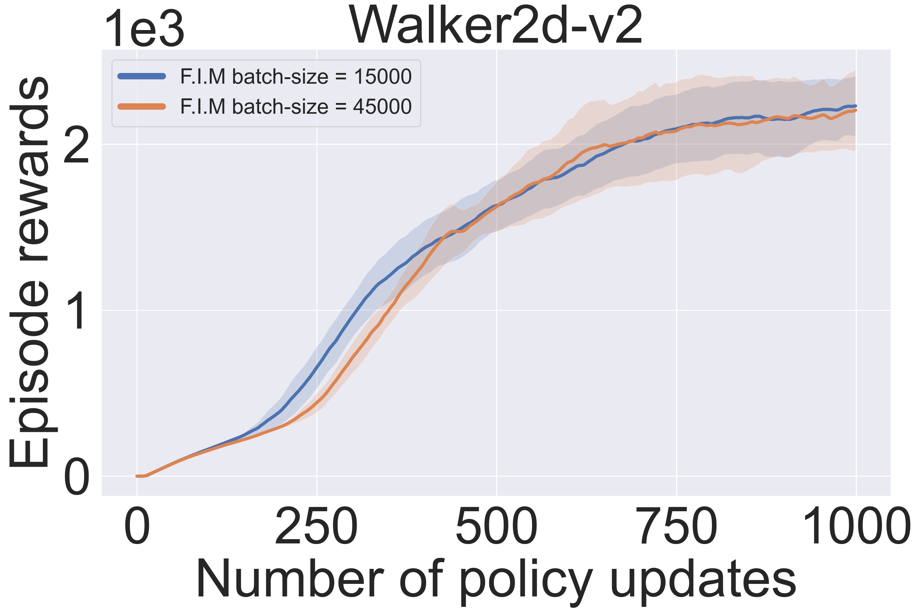
The analytical solution for ${\bm{L}}_{{\bm{\theta}}}^{BQ}$ is obtained by assuming that the Fisher information matrix ${\bm{G}}$ is estimated exactly. However, the practical DBQPG method estimates ${\bm{G}}$ (in the Fisher kernel $k_{f}$) from samples using the Monte-Carlo method (Eq. 19). Here, we investigate the affect of MC approximation of ${\bm{G}}$ on the BQ-PG performance, by estimating ${\bm{G}}$ using $3\times$ more samples than BQ-PG sample size. It can be seen from Fig. 5 that increasing the sample-size of MC approximation of ${\bm{G}}$ does not appreciably improve the performance. As a result, while it is possible to replace the MC approximation of ${\bm{G}}$ matrix with a more efficient numerical integration method (like BQ), we do not expect to see significant improvements over the MC estimation baseline for the ${\bm{G}}$ matrix.

Figure 5: Vanilla PG experiment with DBQPG estimator and 15000 sample size, while estimating the F.I.M ${\bm{G}}$ using (i) 15000 and (ii) 45000 samples.

Appendix E UAPG: From Theory to Practice

PG estimation from samples offers stochastic gradient estimates with a non-uniform gradient uncertainty, i.e., the PG estimator is more uncertain about the gradient’s step size along some directions over others. Due to this inherent disparity in the uncertainty of different gradient components, using a constant learning rate occasionally results in large policy updates along directions of high uncertainty, and consequently a catastrophic performance degradation. Thus, PG algorithms that use MC-PG or DBQPG estimation treat stochastic gradient estimates as the true gradient, making them vulnerable to bad policy updates. UAPG uses DBQPG’s gradient uncertainty ${\bm{C}}_{{\bm{\theta}}}^{BQ}$ to normalize the different components of a DBQPG estimate based on their respective uncertainties, bring all the gradient components to the same scale. In other words, UAPG offers gradient estimates with uniform uncertainty, i.e. gradient covariance is the identity matrix. In theory, the UAPG update is defined as follows:

$${\bm{L}}_{{\bm{\theta}}}^{UAPG} =\big{(}{\bm{C}}_{{\bm{\theta}}}^{BQ}\big{)}^{-\frac{1}{2}}{\bm{L}}_{{\bm{\theta}}}^{BQ},\quad\text{such that}$$ (34)

$${\bm{C}}_{{\bm{\theta}}}^{UAPG} =\big{(}{\bm{C}}_{{\bm{\theta}}}^{BQ}\big{)}^{-\frac{1}{2}}{\bm{C}}_{{\bm{\theta}}}^{BQ}\big{(}{\bm{C}}_{{\bm{\theta}}}^{BQ}\big{)}^{-\frac{1}{2}}={\bm{I}}.$$

However, the empirical ${\bm{C}}_{{\bm{\theta}}}^{BQ}$ estimates are often ill-conditioned matrices (spectrum decays quickly) with a numerically unstable inversion. Since ${\bm{C}}_{{\bm{\theta}}}^{BQ}$ only provides a good estimate of the top few directions of uncertainty, the UAPG update is computed from a rank-$\delta$ singular value decomposition (SVD) approximation of ${\bm{C}}_{{\bm{\theta}}}^{BQ}\approx\nu_{\delta}{\bm{I}}+\sum_{i=1}^{\delta}{\bm{h}}_{i}(\nu_{i}-\nu_{\delta}){\bm{h}}_{i}^{\top}$ as,

$${\bm{L}}_{{\bm{\theta}}}^{UAPG}=\nu_{\delta}^{-\frac{1}{2}}\big{(}{\bm{I}}+\sum\nolimits_{i=1}^{\delta}{\bm{h}}_{i}\big{(}\sqrt{{\nu_{\delta}}/{\nu_{i}}}-1\big{)}{\bm{h}}_{i}^{\top}\big{)}{\bm{L}}_{{\bm{\theta}}}^{BQ}.$$ (35)

The computational complexity of the randomized SVD operation is $\mathcal{O}(2\delta\mathcal{M}+\delta^{2}|\Theta|+\delta^{2}n)$, where $\mathcal{M}$ is the computational complexity of the MVM operation. Using the fast kernel computation methods mentioned earlier, the complexity of MVM operation $\mathcal{M}$ and, subsequently, the randomized SVD algorithm reduces to linear in the number of policy parameters $|\Theta|$ and the sample-size $n$ (see Fig. 6 for empirical evidence).

On the other hand, for the natural policy gradient update ${\bm{L}}^{NBQ}_{{\bm{\theta}}}={\bm{G}}^{-1}{\bm{L}}^{BQ}_{{\bm{\theta}}}$, the gradient uncertainty ${\bm{C}}^{NBQ}_{{\bm{\theta}}}$ is,

$${\bm{C}}_{{\bm{\theta}}}^{NBQ} ={\bm{G}}^{-1}{\bm{C}}_{{\bm{\theta}}}^{BQ}{\bm{G}}^{-1}$$

$$=c_{2}({\bm{G}}^{-1}-c_{2}{\bm{G}}^{-1}{\bm{U}}\Big{(}c_{1}{\bm{K}}_{s}+c_{2}{\bm{K}}_{f}+\sigma^{2}{\bm{I}}\Big{)}^{-1}{\bm{U}}^{\top}{\bm{G}}^{-1})$$

$$=c_{2}({\bm{G}}+c_{2}{\bm{U}}\left(c_{1}{\bm{K}}_{s}+\sigma^{2}{\bm{I}}\right)^{-1}{\bm{U}}^{\top})^{-1},$$ (36)

and the ideal UAPG update is ${\bm{L}}^{NUAPG}_{{\bm{\theta}}}=\left({\bm{C}}^{NBQ}_{{\bm{\theta}}}\right)^{-\frac{1}{2}}{\bm{G}}^{-1}{\bm{L}}^{BQ}_{{\bm{\theta}}}$. However, since ${\bm{C}}_{{\bm{\theta}}}^{NBQ}$ is the inverse of an ill-conditioned matrix, the singular values corresponding to the high-uncertainty directions of ${\bm{C}}_{{\bm{\theta}}}^{NBQ}$ show very little variation in uncertainty. Thus, we instead apply a low-rank approximation on ${{\bm{C}}_{{\bm{\theta}}}^{NBQ}}^{-1}\approx\nu_{\delta}{\bm{I}}+\sum_{i=1}^{\delta}{\bm{h}}_{i}(\nu_{i}-\nu_{\delta}){\bm{h}}_{i}^{\top}$ for the UAPG update of NPG:

$${\bm{L}}_{{\bm{\theta}}}^{NUAPG}=\nu_{\delta}^{\frac{1}{2}}\Big{(}{\bm{I}}+\sum\nolimits_{i=1}^{\delta}{\bm{h}}_{i}\big{(}\min\big{(}\sqrt{{\nu_{i}}/{\nu_{\delta}}},{\epsilon}\big{)}-1\big{)}{\bm{h}}_{i}^{\top}\Big{)}{\bm{G}}^{-1}{\bm{L}}_{{\bm{\theta}}}^{BQ},\qquad{\epsilon}>1$$ (37)

Note that ${{\bm{C}}^{NBQ}_{{\bm{\theta}}}}^{-1}$ is an ill-conditioned matrix whose top $\delta$ PCs denote the least uncertain/most confident directions of natural gradient estimation (equivalent to the bottom $\delta$ PCs of ${\bm{C}}^{NBQ}_{{\bm{\theta}}}$). Further, we replace $\sqrt{{\nu_{i}}/{\nu_{\delta}}}$ with $\min(\sqrt{{\nu_{i}}/{\nu_{\delta}}},{\epsilon})$ in Eq. 37 to avoid taking large steps along these directions, solely on the basis of their uncertainty. Thus, for NPG estimates, UAPG offers a more reliable policy update direction by relatively increasing the step size along the most confident directions (i.e., the top $\delta$ PCs of ${{\bm{C}}_{{\bm{\theta}}}^{NBQ}}^{-1}$), as opposed to lowering the stepsize for the most uncertain directions like in the case of UAPG over Vanilla PG estimates.

E.1 Relation between the Gradient Uncertainties of Vanilla PG and NPG

Empirically, we found that the optimal value of $c_{2}\ll 1$, at which point, the gradient uncertainty of Vanilla PG and Natural PG algorithms approximate to:

$${\bm{C}}_{{\bm{\theta}}}^{BQ} =c_{2}{\bm{G}}-c_{2}^{2}{\bm{U}}(c_{1}{\bm{K}}_{s}+c_{2}{\bm{K}}_{f}+\sigma^{2}{\bm{I}})^{-1}{\bm{U}}^{\top}\approx c_{2}{\bm{G}},$$ (38)

$${\bm{C}}_{{\bm{\theta}}}^{NBQ} =c_{2}({\bm{G}}+c_{2}{\bm{U}}\left(c_{1}{\bm{K}}_{s}+\sigma^{2}{\bm{I}}\right)^{-1}{\bm{U}}^{\top})^{-1}\approx c_{2}{{\bm{G}}}^{-1}.$$ (39)

This observation is particularly interesting because for $c_{2}\ll 1$, most uncertain gradient directions for vanilla PG approximately correspond to the most confident (least uncertain) directions for NPG. Crudely speaking, the natural gradient takes the step size along each direction and divides it by the estimated variance (from the gradient covariance matrix), which results in an inversion of the uncertainty. In contrast, UAPG divides the stepsize along each direction by the estimated standard deviation, which results in uniform uncertainty along all the directions. Moreover, for $c_{2}\ll 1$, the ideal UAPG update for both vanilla PG and NPG converges along the ${\bm{G}}^{-\frac{1}{2}}{\bm{L}}_{{\bm{\theta}}}^{BQ}$ direction.

Appendix F Wall-Clock Performance of DBQPG and UAPG

Figure 6: Wall-Clock time for PG estimation using MC, DBQPG and UAPG methods on HumanoidStandup-v2 environment.

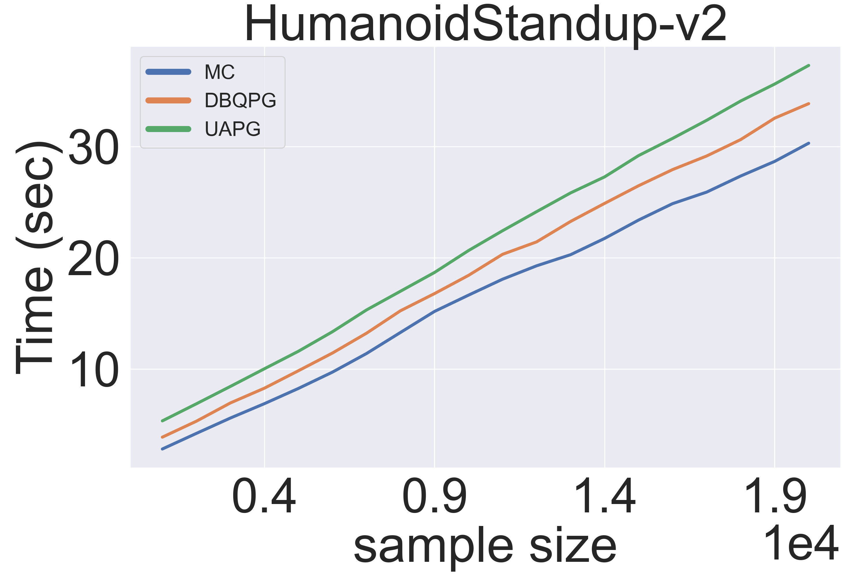
The wall-clock time for PG estimation using MC, DBQPG and UAPG, on “HumanoidStandup-v2” environment (376-d state and 17-d action space) is reported in Fig. 6. Clearly, DBQPG and UAPG methods have a negligible computational overhead over MC-PG, while being significantly more sample efficient (Fig. 9). Further, it is also clear from the plot that the wall-clock time of MC, DBQPG and UAPG methods increases linearly in sample size $n$, which agrees with our complexity analysis in Sec. 4 (main paper).

Appendix G Comparison with Prior BQ-PG works

Engel, Mannor, and Meir (2003) is one of the first RL approaches to use GPs for approximating the action-value function $Q_{\pi_{{\bm{\theta}}}}$. The Bayesian deep Q-networks (BDQN) (Azizzadenesheli and Anandkumar 2018) extends this idea to high-dimensional domains with a discrete action space. More specifically, BDQN uses Bayesian linear regression, i.e., a parametric GP with a linear kernel, instead of linear regression to learn the last layer in a standard DQN architecture. BDQN then uses the uncertainty modeled by the GP to perform Thompson sampling on the learned posterior distribution for efficiently balancing exploration and exploitation. Like in BDQN, the implicit GP critic in DBQPG can also be seen as a standard deep critic network with its final linear layer substituted by a non-parametric GP layer.

Figure 7: (left) Ablation study to investigate the role of different components of DBQPG, and (right) Comparison between common state kernel $k_{s}$ choices.

The DBQPG algorithm is an extension of the (sequential) Bayesian Actor-Critic (BAC) algorithm (Ghavamzadeh and Engel 2007) that leverages the automatic differentiation framework and fast kernel computation methods for PG estimation from a batch of samples (parallel), thus placing the BQ-PG framework in the context of contemporary PG algorithms. Aside from this, DBQPG also replaces the traditional inducing points framework (Silverman 1985) ($\mathcal{O}(m^{2}n+m^{3})$ time and $\mathcal{O}(mn+m^{2})$ storage complexity) used in BAC, with a more computationally-efficient alternative, SKI ($\mathcal{O}(n+m^{2})$ time and storage). Moreover, DBQPG boosts the expressive power of base (state) kernel with a deep neural network, followed by kernel learning its parameters (Eq. 9, main paper).

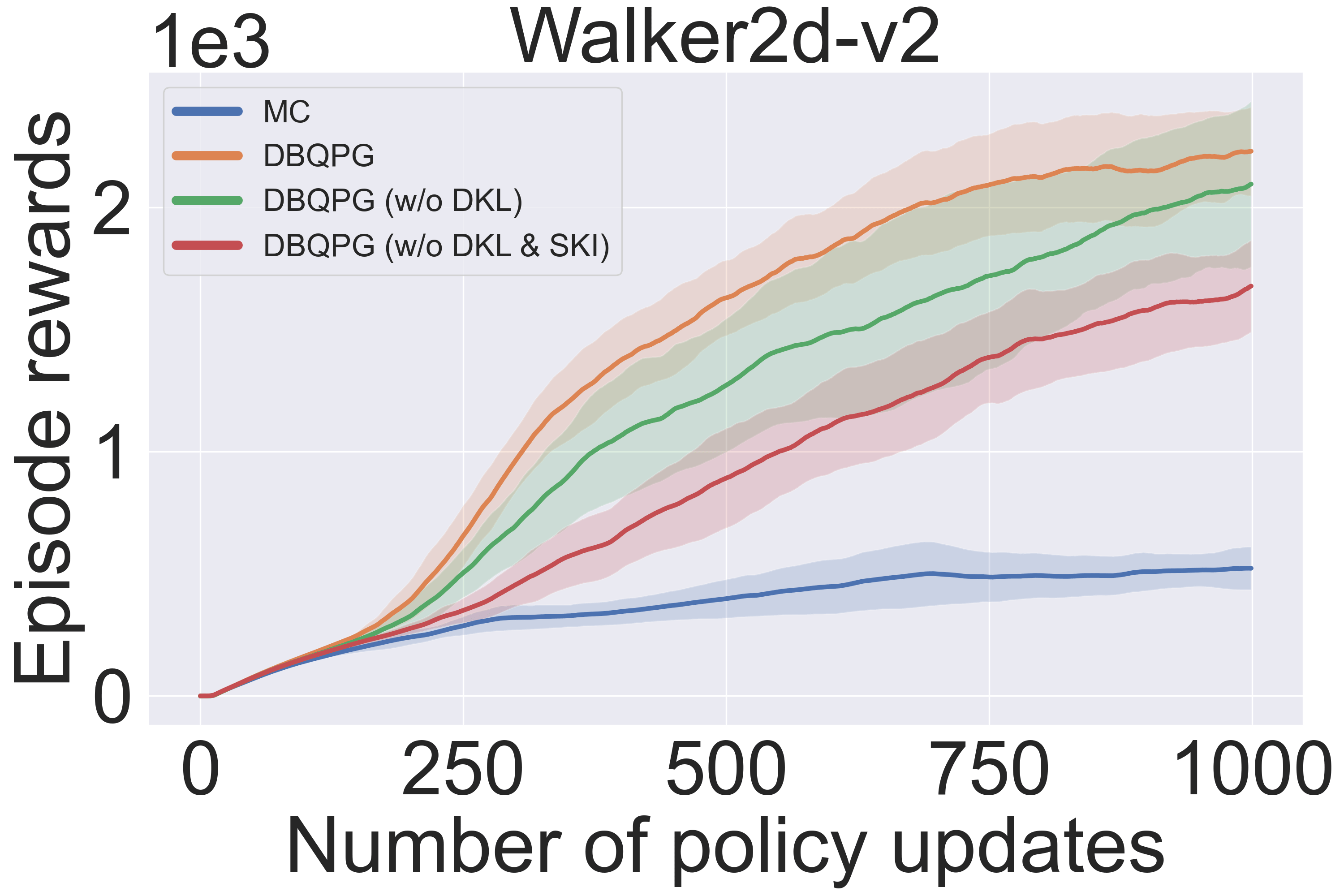
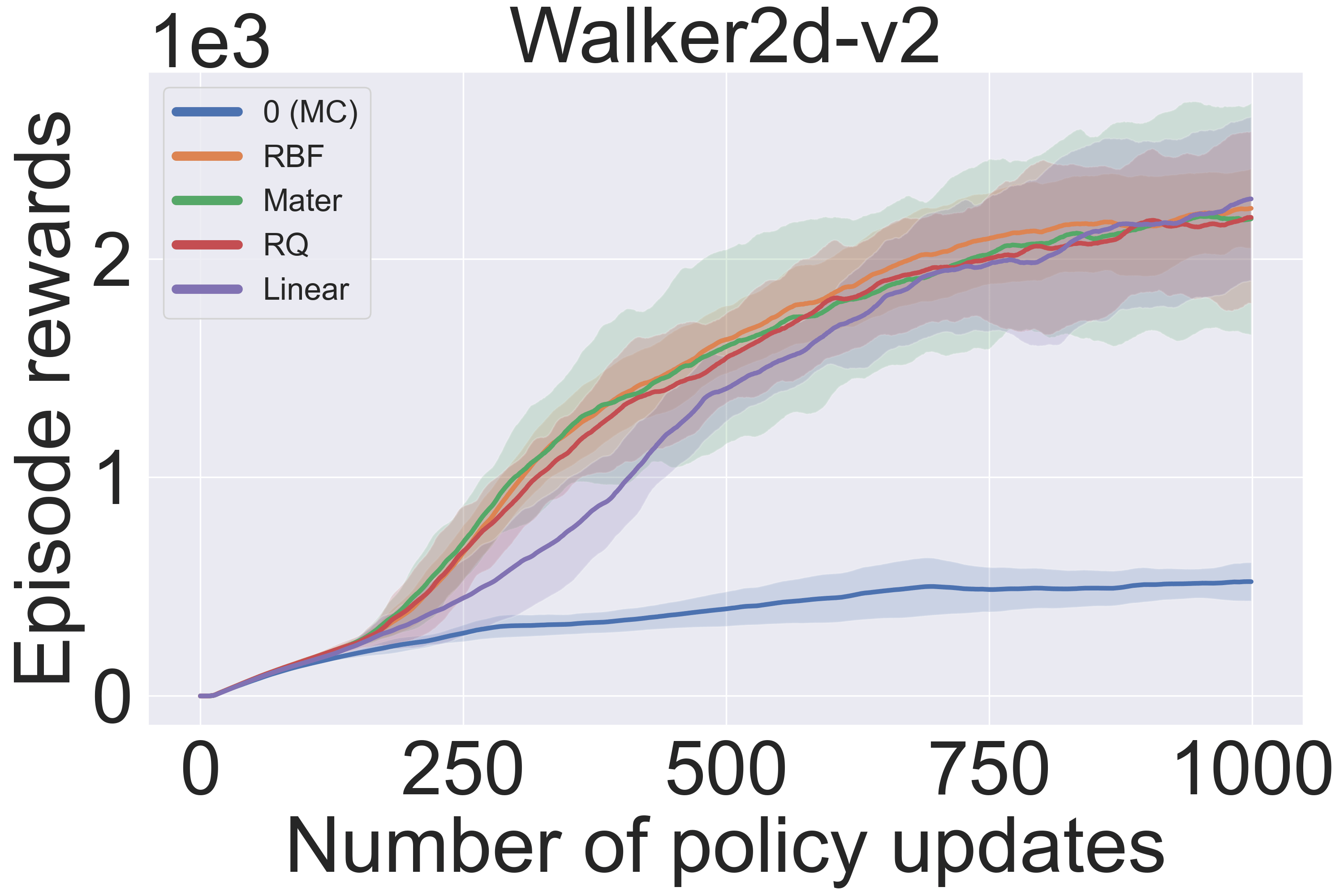
Switching from deep kernel back to a base kernel (DBQPG (w/o DKL)) corresponds to a noticeable drop in performance as shown in Fig. 7 (left). Moreover, replacing the SKI approximation with a traditional inducing points method (DBQPG (w/o DKL & SKI)) further lowers the performance. Here, “DBQPG (w/o DKL & SKI)” can be thought of as the reimplementation of BAC in batch settings (parallel computation). Interestingly, BAC (ours), i.e. DBQPG (w/o DKL & SKI), still manages to outperform the MC-PG baseline. Further, Fig. 7 (middle) suggests that most popular base kernels, when coupled with a DNN feature extractor, provide nearly similar performance, while easily outperforming the MC-PG baseline. This observation suggests that a deep (state) kernel with any of the popular base kernel choices is often a better prior that the trivial state kernel $k_{s}=0$, which corresponds to MC-PG.

Figure 8: UAPG versus the uncertainty-based policy update proposed in Ghavamzadeh, Engel, and Valko (2016).

Further, Ghavamzadeh, Engel, and Valko (2016) introduces an extension of BAC that uses the gradient covariance ${\bm{C}}_{{\bm{\theta}}}^{BQ}$ for adjusting the learning rate of policy parameters:

$${\bm{L}}_{{\bm{\theta}}}^{UBAC}=\left({\bm{I}}-\frac{1}{\nu_{0}}{\bm{C}}_{{\bm{\theta}}}^{BQ}\right){\bm{L}}_{{\bm{\theta}}}^{BQ},$$ (40)

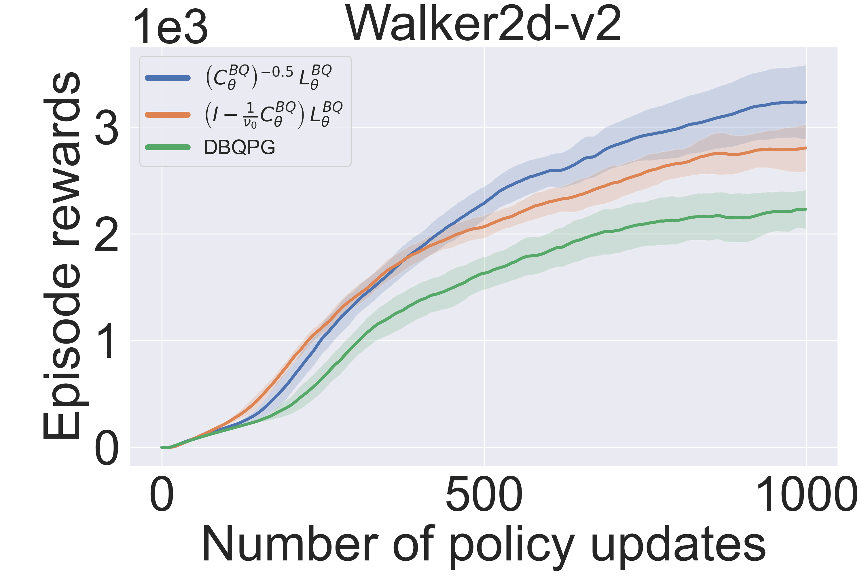
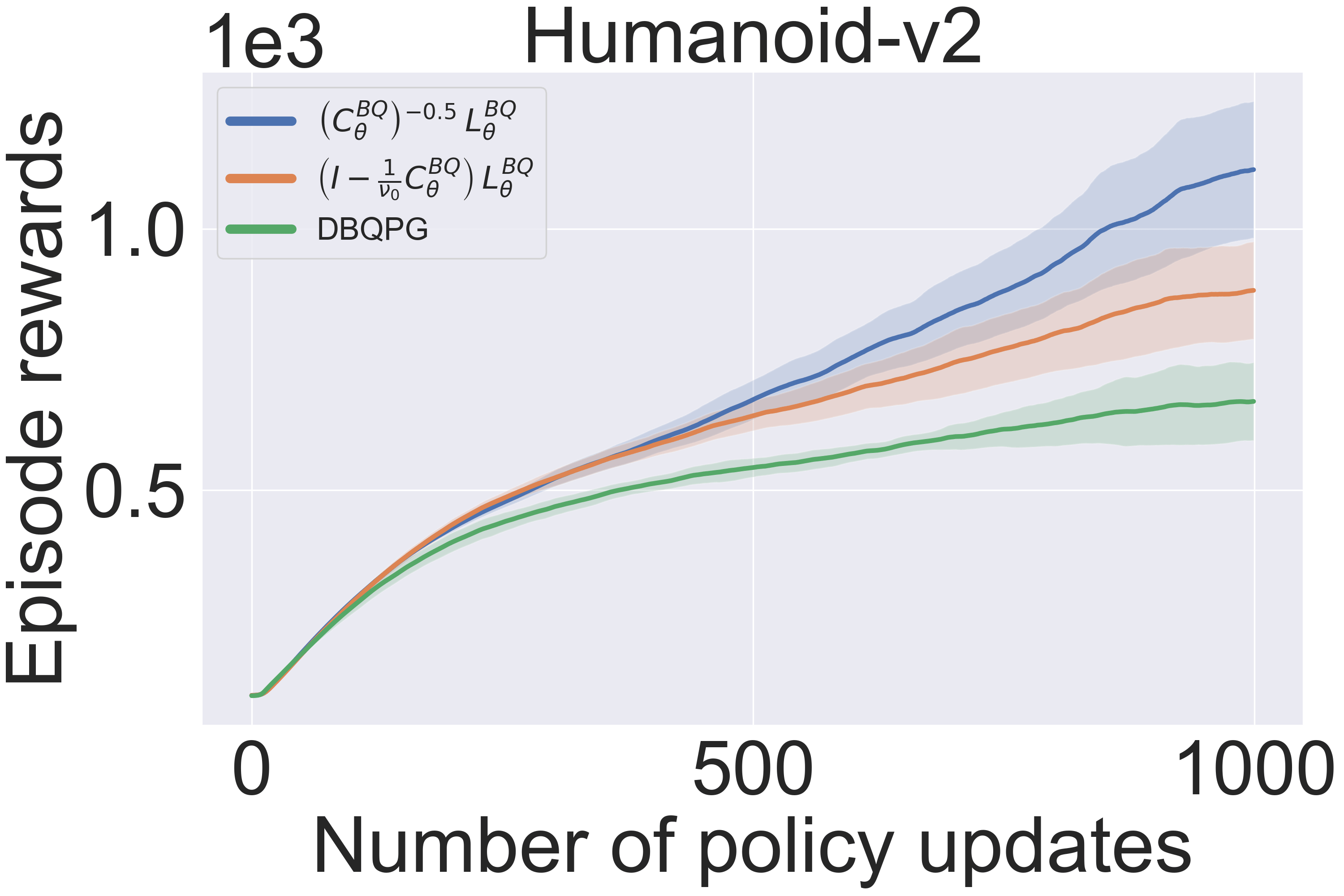
where $\nu_{0}$ is the largest singular value of ${\bm{C}}_{{\bm{\theta}}}^{BQ}$. This gradient preconditioning is one of the many possible solutions to lower the step-size of gradient components with high uncertainties, with another solution being UAPG. However, UAPG update satisfies a more stricter condition of providing policy updates with uniform uncertainty. Since, ${\bm{L}}_{{\bm{\theta}}}^{UBAC}$ does not provide PG estimates with uniform uncertainty, it is more vulnerable to bad policy updates than UAPG. This is also demonstrated in practice, where ${\bm{L}}_{{\bm{\theta}}}^{UAPG}$ outperforms ${\bm{L}}_{{\bm{\theta}}}^{UBAC}$, while both the uncertainty-based methods outperform DBQPG (see Fig. 8). Moreover, ${\bm{L}}_{{\bm{\theta}}}^{UBAC}$ update would not work for NPG and TRPO algorithms as their covariance is the inverse of an ill-conditioned matrix.

Appendix H Implementation Details

We follow the architecture from Fig. 1 (left; main paper), where the policy $\pi_{\bm{\theta}}$ comprises of a deep neural network that takes the observed state as input and estimates a normal distribution in the output action-space, characterized by the mean and standard deviation. We use the standard policy network architecture (Schulman et al. 2015; Duan et al. 2016) that comprises of a $2$-layered fully-connected MLP with $64$ hidden units and a tanh non-linearity in each layer. Our state feature extractor $\phi(s)$ is another MLP with hidden dimensions $64$, $48$, and $10$, and tanh non-linearity. The explicit critic network is simply a linear layer with $1$ output unit, on top of the $10$-d output of $\phi(s)$. The explicit critic models the state-value function $V_{\pi_{\bm{\theta}}}$ and its parameters are optimized for TD error. The $n$ dimensional vector ${\bm{Q}}$ is formed from generalized advantage estimates (Schulman et al. 2016), which are computed using MC estimates of return and the state-value predictions offered by the explicit critic network.

The implicit GP critic implicitly models the generalized advantage function using the samples ${\bm{Q}}$, a fisher kernel (no additional hyperparameters; derived directly from the policy parameters) and a deep RBF state kernel (lengthscale + $\phi(s)$ parameters). For structured kernel interpolation (Wilson and Nickisch 2015), we use a grid size of $128$ and impose an additive structure (i.e. the overall kernel is the sum of individual RBF kernels along each input dimension) on the deep RBF kernel. Additive structure allows us to take advantage of the Toeplitz method (Turner 2010) for fast and scalable MVM computation. The GP’s noise variance $\sigma^{2}$ is set to $10^{-4}$. In all the experiments of BQ-based methods, we fixed the hyperparameters $c_{1}=1$ and $c_{2}=5\times 10^{-5}$ (tuned values). The parameters of deep RBF kernel are optimized for GP-MLL objective (Eq. 9). Since $\phi(s)$ is shared between the implicit critic (deep RBF kernel) and explicit critic, its parameters are updated for both GP-MLL and TD error objectives. Our implementation is based on GPyTorch (Gardner et al. 2018), a software package for scalable GP inference with GPU acceleration support.

For Vanilla PG and NPG experiments, we used the ADAM optimizer (Kingma and Ba 2015) to update the policy network. In the UAPG experiments, increasing the SVD rank $\delta$ pushes the practical UAPG estimate closer to the ideal UAPG estimate, while, also increases the GPU memory requirement. We balance this trade-off for each environment by choosing a $\delta$ that closely approximates the initial spectrum of gradient uncertainty ${\bm{C}}^{BQ}_{{\bm{\theta}}}$ and also has a favorable GPU memory consumption. Lastly, we set ${\epsilon}=3$ for UAPG’s natural gradient update. Our implementation of DBQPG and UAPG methods is made publicly available at https://github.com/Akella17/Deep-Bayesian-Quadrature-Policy-Optimization.

Parameter Value Batch size $15000$ Discount factor $\gamma$ $0.995$ GAE coefficient $\tau$ $0.97$ Trust region constraint / step size $0.01$ Conjugate Gradient Max. CG iterations $50$ Residue (i.e., CG Threshold) $10^{-10}$ Damping (stability) factor $0.1$

Table 1: Common hyperparameter setting across all the experiments.

Vanilla PG

NPG

TRPO

Figure 9: Full comparison of BQ-based methods and MC estimation in vanilla PG, NPG, and TRPO frameworks across $7$ MuJoCo environments. The agent’s performance is averaged over $10$ runs.

References

- Agarwal et al. (2019) Agarwal, A.; Kakade, S. M.; Lee, J. D.; and Mahajan, G. 2019. Optimality and approximation with policy gradient methods in markov decision processes. arXiv preprint arXiv:1908.00261 .
- Azizzadenesheli and Anandkumar (2018) Azizzadenesheli, K.; and Anandkumar, A. 2018. Efficient Exploration through Bayesian Deep Q-Networks. arXiv preprint arXiv:1802.04412 .
- Baxter and Bartlett (2000) Baxter, J.; and Bartlett, P. L. 2000. Direct gradient-based reinforcement learning. In 2000 IEEE International Symposium on Circuits and Systems. Emerging Technologies for the 21st Century. Proceedings (IEEE Cat No. 00CH36353), volume 3, 271–274. IEEE.
- Briol et al. (2015) Briol, F.-X.; Oates, C.; Girolami, M.; and Osborne, M. A. 2015. Frank-Wolfe Bayesian quadrature: Probabilistic integration with theoretical guarantees. In Advances in Neural Information Processing Systems, 1162–1170.
- Brockman et al. (2016) Brockman, G.; Cheung, V.; Pettersson, L.; Schneider, J.; Schulman, J.; Tang, J.; and Zaremba, W. 2016. OpenAI Gym.
- Duan et al. (2016) Duan, Y.; Chen, X.; Houthooft, R.; Schulman, J.; and Abbeel, P. 2016. Benchmarking Deep Reinforcement Learning for Continuous Control. In Proceedings of the 33rd International Conference on International Conference on Machine Learning - Volume 48, ICML’16, 1329–1338. JMLR.org. URL http://dl.acm.org/citation.cfm?id=3045390.3045531.
- Engel, Mannor, and Meir (2003) Engel, Y.; Mannor, S.; and Meir, R. 2003. Bayes Meets Bellman: The Gaussian Process Approach to Temporal Difference Learning. In Proceedings of the Twentieth International Conference on International Conference on Machine Learning, ICML’03, 154–161. AAAI Press. ISBN 1-57735-189-4. URL http://dl.acm.org/citation.cfm?id=3041838.3041858.
- Engel, Mannor, and Meir (2005) Engel, Y.; Mannor, S.; and Meir, R. 2005. Reinforcement Learning with Gaussian Processes. In Proceedings of the 22Nd International Conference on Machine Learning, ICML ’05, 201–208. New York, NY, USA: ACM. ISBN 1-59593-180-5. doi:10.1145/1102351.1102377. URL http://doi.acm.org/10.1145/1102351.1102377.
- Gardner et al. (2018) Gardner, J. R.; Pleiss, G.; Bindel, D.; Weinberger, K. Q.; and Wilson, A. G. 2018. GPyTorch: Blackbox Matrix-matrix Gaussian Process Inference with GPU Acceleration. In Proceedings of the 32Nd International Conference on Neural Information Processing Systems, NIPS’18, 7587–7597. USA: Curran Associates Inc. URL http://dl.acm.org/citation.cfm?id=3327757.3327857.
- Ghavamzadeh and Engel (2006) Ghavamzadeh, M.; and Engel, Y. 2006. Bayesian Policy Gradient Algorithms. In Proceedings of the 19th International Conference on Neural Information Processing Systems, NIPS’06, 457–464. Cambridge, MA, USA: MIT Press.
- Ghavamzadeh and Engel (2007) Ghavamzadeh, M.; and Engel, Y. 2007. Bayesian Actor-critic Algorithms. In Proceedings of the 24th International Conference on Machine Learning, ICML ’07, 297–304. New York, NY, USA: ACM. ISBN 978-1-59593-793-3. doi:10.1145/1273496.1273534. URL http://doi.acm.org/10.1145/1273496.1273534.
- Ghavamzadeh, Engel, and Valko (2016) Ghavamzadeh, M.; Engel, Y.; and Valko, M. 2016. Bayesian Policy Gradient and Actor-Critic Algorithms. Journal of Machine Learning Research 17(66): 1–53. URL http://jmlr.org/papers/v17/10-245.html.
- Halko, Martinsson, and Tropp (2011) Halko, N.; Martinsson, P.-G.; and Tropp, J. A. 2011. Finding structure with randomness: Probabilistic algorithms for constructing approximate matrix decompositions. SIAM review 53(2): 217–288.
- Hennig, Osborne, and Girolami (2015) Hennig, P.; Osborne, M. A.; and Girolami, M. 2015. Probabilistic numerics and uncertainty in computations. Proceedings of the Royal Society of London A: Mathematical, Physical and Engineering Sciences 471(2179).
- Ilyas et al. (2018) Ilyas, A.; Engstrom, L.; Santurkar, S.; Tsipras, D.; Janoos, F.; Rudolph, L.; and Madry, A. 2018. Are Deep Policy Gradient Algorithms Truly Policy Gradient Algorithms? ArXiv abs/1811.02553.
- Kakade (2001) Kakade, S. 2001. A Natural Policy Gradient. In Proceedings of the 14th International Conference on Neural Information Processing Systems: Natural and Synthetic, NIPS’01, 1531–1538. Cambridge, MA, USA: MIT Press. URL http://dl.acm.org/citation.cfm?id=2980539.2980738.
- Kakade and Langford (2002) Kakade, S.; and Langford, J. 2002. Approximately optimal approximate reinforcement learning. In ICML, volume 2, 267–274.
- Kanagawa, Sriperumbudur, and Fukumizu (2016) Kanagawa, M.; Sriperumbudur, B. K.; and Fukumizu, K. 2016. Convergence guarantees for kernel-based quadrature rules in misspecified settings. In Advances in Neural Information Processing Systems, 3288–3296.
- Kanagawa, Sriperumbudur, and Fukumizu (2020) Kanagawa, M.; Sriperumbudur, B. K.; and Fukumizu, K. 2020. Convergence analysis of deterministic kernel-based quadrature rules in misspecified settings. Foundations of Computational Mathematics 20(1): 155–194.
- Kingma and Ba (2015) Kingma, D. P.; and Ba, J. L. 2015. Adam: A Method for Stochastic Optimization. international conference on learning representations (2015) .
- Konda and Tsitsiklis (2000) Konda, V. R.; and Tsitsiklis, J. N. 2000. Actor-Critic Algorithms. In Solla, S. A.; Leen, T. K.; and Müller, K., eds., Advances in Neural Information Processing Systems 12, 1008–1014. MIT Press. URL http://papers.nips.cc/paper/1786-actor-critic-algorithms.pdf.
- Konda and Tsitsiklis (2003) Konda, V. R.; and Tsitsiklis, J. N. 2003. On Actor-Critic Algorithms. SIAM J. Control Optim. 42(4): 1143–1166. ISSN 0363-0129. doi:10.1137/S0363012901385691. URL https://doi.org/10.1137/S0363012901385691.
- Lillicrap et al. (2015) Lillicrap, T. P.; Hunt, J. J.; Pritzel, A.; Heess, N.; Erez, T.; Tassa, Y.; Silver, D.; and Wierstra, D. 2015. Continuous control with deep reinforcement learning. arXiv preprint arXiv:1509.02971 .
- Metropolis and Ulam (1949) Metropolis, N.; and Ulam, S. 1949. The monte carlo method. Journal of the American statistical association 44(247): 335–341.
- Micchelli, Xu, and Zhang (2006) Micchelli, C. A.; Xu, Y.; and Zhang, H. 2006. Universal Kernels. J. Mach. Learn. Res. 7: 2651–2667. ISSN 1532-4435.
- O’Hagan (1991) O’Hagan, A. 1991. Bayes-Hermite quadrature. Journal of Statistical Planning and Inference 29(3): 245–260. URL http://www.sciencedirect.com/science/article/B6V0M-45F5GDM-53/1/6e05220bfd4a6174e890f60bb391107c.
- Peters and Schaal (2008) Peters, J.; and Schaal, S. 2008. Reinforcement Learning of Motor Skills with Policy Gradients. Neural Networks 21(4): 682–697.
- Rasmussen and Williams (2005) Rasmussen, C. E.; and Williams, C. K. I. 2005. Gaussian Processes for Machine Learning (Adaptive Computation and Machine Learning). The MIT Press. ISBN 026218253X.
- Reisinger, Stone, and Miikkulainen (2008) Reisinger, J.; Stone, P.; and Miikkulainen, R. 2008. Online Kernel Selection for Bayesian Reinforcement Learning. In Proceedings of the 25th International Conference on Machine Learning, ICML ’08, 816–823. New York, NY, USA: Association for Computing Machinery. ISBN 9781605582054. doi:10.1145/1390156.1390259. URL https://doi.org/10.1145/1390156.1390259.
- Rubinstein (1969) Rubinstein, R. Y. 1969. Some Problems in Monte Carlo Optimization. Ph.D. thesis .
- Saatci (2012) Saatci, Y. 2012. Scalable Inference for Structured Gaussian Process Models. University of Cambridge. URL https://books.google.co.in/books?id=9pC3oQEACAAJ.
- Schulman et al. (2015) Schulman, J.; Levine, S.; Moritz, P.; Jordan, M. I.; and Abbeel, P. 2015. Trust Region Policy Optimization. In Proceedings of the 32nd International Conference on Machine Learning (ICML).
- Schulman et al. (2016) Schulman, J.; Moritz, P.; Levine, S.; Jordan, M.; and Abbeel, P. 2016. High-Dimensional Continuous Control Using Generalized Advantage Estimation. In Proceedings of the International Conference on Learning Representations (ICLR).
- Silverman (1985) Silverman, B. W. 1985. Some Aspects of the Spline Smoothing Approach to Non-Parametric Regression Curve Fitting. Journal of the Royal Statistical Society. Series B (Methodological) 47(1): 1–52. ISSN 00359246. URL http://www.jstor.org/stable/2345542.
- Sutton et al. (2000) Sutton, R. S.; McAllester, D.; Singh, S.; and Mansour, Y. 2000. Policy Gradient Methods for Reinforcement Learning with Function Approximation. In Proceedings of the 12th International Conference on Neural Information Processing Systems, NIPS’99, 1057–1063. Cambridge, MA, USA: MIT Press. URL http://dl.acm.org/citation.cfm?id=3009657.3009806.
- Todorov, Erez, and Tassa (2012) Todorov, E.; Erez, T.; and Tassa, Y. 2012. Mujoco: A physics engine for model-based control. In 2012 IEEE/RSJ International Conference on Intelligent Robots and Systems, 5026–5033. IEEE.
- Townsend (2017) Townsend, J. 2017. A new trick for calculating Jacobian vector products. URL https://j-towns.github.io/2017/06/12/A-new-trick.html.
- Turner (2010) Turner, R. E. 2010. Statistical Models for Natural Sounds. Ph.D. thesis, Gatsby Computational Neuroscience Unit, UCL.
- Williams (1992) Williams, R. J. 1992. Simple Statistical Gradient-Following Algorithms for Connectionist Reinforcement Learning. Mach. Learn. 8(3-4): 229–256. ISSN 0885-6125. doi:10.1007/BF00992696. URL https://doi.org/10.1007/BF00992696.
- Wilson et al. (2016) Wilson, A. G.; Hu, Z.; Salakhutdinov, R.; and Xing, E. P. 2016. Deep Kernel Learning. In Gretton, A.; and Robert, C. C., eds., Proceedings of the 19th International Conference on Artificial Intelligence and Statistics, volume 51 of Proceedings of Machine Learning Research, 370–378. Cadiz, Spain: PMLR. URL http://proceedings.mlr.press/v51/wilson16.html.
- Wilson and Nickisch (2015) Wilson, A. G.; and Nickisch, H. 2015. Kernel Interpolation for Scalable Structured Gaussian Processes (KISS-GP). In Proceedings of the 32Nd International Conference on International Conference on Machine Learning - Volume 37, ICML’15, 1775–1784. JMLR.org. URL http://dl.acm.org/citation.cfm?id=3045118.3045307.
- Woodbury (1950) Woodbury, M. A. 1950. Inverting modified matrices. Memorandum report 42(106): 336.
- Zhao et al. (2011) Zhao, T.; Hachiya, H.; Niu, G.; and Sugiyama, M. 2011. Analysis and Improvement of Policy Gradient Estimation. In Shawe-Taylor, J.; Zemel, R. S.; Bartlett, P. L.; Pereira, F.; and Weinberger, K. Q., eds., Advances in Neural Information Processing Systems 24, 262–270. Curran Associates, Inc.