Massive particle pair production and oscillation in Friedman Universe: reheating energy and entropy, and cold dark matter
Abstract
Suppose that the early Universe starts with a cosmological -term originating from quantum spacetime at the Planck scale. Dark energy drives inflation and reheating by reducing its value for massive particle-antiparticle pairs production and oscillation, resulting in a holographic and massive pair plasma state. The back-and-forth reaction of dark energy and massive pairs slows inflation to its end and starts reheating by rapidly producing stable and unstable pairs. We introduce the Boltzmann-type rate equation describing the back-and-forth reaction. It forms a close set with Friedman equations and reheating equations for unstable pairs decay to relativistic particles. The numerical solutions show preheating, massive pairs dominated and genuine reheating episodes. We obtain the reheating temperature and entropy in terms of the tensor-to-scalar ratio consistently with observations. Stable massive pairs represent cold dark matter particles and weakly interact with dark energy. The resultant cold dark matter abundance is about a constant in time.
1 Introduction
In the standard model of modern cosmology (CDM), the cosmological constant , dark matter, inflation, reheating and coincidence problem have been long-standing basic issues for decades. The inflation [1, 2, 3, 4, 5, 6, 7] reheating [8, 9, 10, 11, 12, 13, 14, 15, 16, 17] are fundamental processes. The latter transition the Universe from the cold and massive state left by inflation to the hot Big Bang, and then the standard cosmology follows. The evolution follows the Friedman equations of cosmological , matter and radiation energy densities. The cosmological and massive particle origin are still mysteries. One calls them “dark energy” and “cold dark matter”. Moreover, their properties and interactions in the Universe’s evolution are also in question. Why their present values are coincidentally in the same order of magnitude?
To get an insight into these issues, people have been intensively studying the gravitational particle production in Friedman Universe for decades [19, 20, 21, 22, 23, 24, 25, 26, 27, 28, 29, 30, 31, 32]. Based on the adiabatic and non-back-reaction approximation for a slowly time-varying Hubble function , one adopted the semi-classical approaches to calculating the particle production rate. It is exponentially suppressed for massive particles since the classical Universe evolution time scale is much larger than the quantum time scale of particle production. However, the non-adiabatic back-reactions of massive particle productions on the Hubble function can be large. One has to take them into account. People have made many efforts [23, 33, 34, 35, 36, 37, 38, 39, 40, 41] to study non-adiabatic back-reaction and understand massive particle productions without exponential suppression. To properly include the back-reaction of particle production on Universe evolution, one should separate fast components from slow components in the Friedman equation. Here, the fast components represent fluctuating gravitational and particle fields at the time scale . The slow components represent slowly varying background fields and particle densities at the time scale .
In Ref. [41], we assume the inflation epoch starts when the dark-energy density is the order of the Planck scale, dominates the Hubble function and the matter density is negligibly small. We study the Universe undergoes a -driven inflation that slowly slows down to its end by producing heavy particles of mass . Inflation is a semi-classical dynamics of the time scale , while massive particle production is a quantum-field dynamics of the time scale . We investigate how the massive particle production density back reacts by separating the fast and slow components in the Friedman equation. Analysis shows and slowly decrease, as slowly increases in time, namely, slowly converts to . It gives the quasi-de Sitter phase (slow-rolling dynamics) for inflation. The final results are consistent with observations. Here we turn to discuss the reheating epoch and possibly explain reheating energy and entropy, as well as cold dark matter, in comparison with current observations.
We review the previous results of the fast and slow components’ separation in Sec. 2, quantum massive pair production and oscillation in Sec. 3, and a massive pair plasma state in Sec. 4. We present in Secs. 5 and 6 the new studies of a complete set of differential equations and initial conditions for the reheating epoch. We numerically solve these equations and compare the results with observations in Secs. 7 and 8. We present preliminary discussions on stable massive as cold dark matter candidate in Sec. 9. is the Newton constant, is the Planck scale and reduced Planck scale GeV.
2 Slow adiabatic and fast non-adiabatic components
We discuss such fast and slow separation in the CDM scenario, where a time-varying cosmological term in the Friedman equation represents such interacting dark energy. The Friedman equations for a flat Universe are [18]
| (2.1) |
where energy density and pressure . The second Equation of (2.1) is the generalised conservation law (Bianchi identity) for including time-varying cosmological term . It reduces to the usual Equation for time-constant . The second Equation of (2.1) shows that and decreases in time, due to the matter’s gravitational attractive nature.
Separating fast components from slow ones [37], we describe the slow and fast components’ decomposition: scale factor , Hubble function , cosmological and matter densities and pressures . The fast components vary faster in time, but their amplitudes are much smaller than the slow ones. According to the order of small ratio of fast and slow components, the Friedman equations (2.1) decompose into two sets. The slow components obey the same equations as usual Friedman equations (“macroscopic” equations)
| (2.2) | |||||
| (2.3) |
where , time derivatives and relate to the macroscopic “slow” time variation scale . The Equation of the state is for normal radiation and matter (including dark matter) components. They enter the usual dynamics of Universe evolution, i.e., inflation, reheating and standard cosmology. The faster components obey “microscopic” equations 111They differ from the equations obtained by scalar field and potential model in Ref [37],
| (2.4) | |||||
| (2.5) |
where the fast components of matter density and pressure are due to the non-adiabatic production of massive particle and antiparticle pairs in fast time variation and its time derivative . They relate to the microscopic “fast” time variation scale . Whereas all slow components approximate as constants “background” in “fast” time variation. The dark-energy equation of state splits into and , and is at the leading order . Approximation sign “” in Eqs. (2.3,2.5) indicates we use 222Here, is due to time-varying dark energy interacting with matter [42]. In contrast, in non-interacting constant case..
The fast and slow components’ separation and coupled Equations (2.2-2.5) are formal and generic. It applies to all Universe’s evolution epochs: inflation, reheating and standard cosmology. However, the fast components (2.4,2.5) depend on the slow components (2.2,2.3) in different evolution epoch. In due course, we will discuss what the fast components and in Eqs. (2.4) and (2.5) are, and how they interact and contribute to the slow components in Friedman equations (2.2) and (2.3).
3 Quantum massive pair production and oscillation
3.1 Quantum massive pair production
In this section, we briefly discuss the Parker and Fulling results [23] for the gravitational production of a large number of massive particles () via non-adiabatic processes. We will re-derive the results in the CDM (2.1) and use them for the fast components of matter density and pressure in Eq. (2.4,2.5).
In Ref. [23], authors discussed the results for boson fields. It is also valid for fermion fields. A quantised massive scalar matter field inside the Hubble sphere volume of Friedman Universe reads
| (3.1) |
Here we consider a massive field and its modes well localise inside the horizon. The field exponentially vanishes outside the horizon , i.e., the particle horizon of comoving Hubble radius. The symbol “” labels quantum states of physical wave vectors , and for the ground state 333In Ref. [23], the principal quantum number is the angular momentum number “” and are the four-dimensional spherical harmonics for the closed Robertson-Walker metric and . The ground state is . Here we discuss the case of a flat Robertson-Walker metric and , for which a massive scalar matter field has no discrete spectra. However, this is not important here since we adopt the Parker-Fulling result (3.6) for the ground state and , which well localizes inside the horizon. . The and are time-independent annihilation and creation operators satisfying the commutation relation . The time-separate equation for is
| (3.2) |
and Wronskian-type condition in the conformal coupling case. Expressing
| (3.3) |
in terms of and , Equation (3.2) becomes
| (3.4) |
and , where . In an adiabatic process for slowly time-varying , the particle state and evolves to and . Positive and negative frequency modes get mixed, leading to particle productions of probability .
We will study particle production in non-adiabatic processes of rapidly time-varying , and . We focus only on the ground state of the lowest-lying massive mode . First, we recall that Parker and Fulling introduced transformation [23],
| (3.5) |
, and two mixing constants obey . For a given and its Fock space, the state is defined by the conditions and
| (3.6) |
The and are time-independent creation and annihilation operators of the pair of mixed positive frequency particles and negative frequency antiparticle. The state contains pairs, and it is the ground state of non-adiabatic interacting system of fast varying and massive pair production and annihilation. It is a coherent superposition of states of a large occupation number of particle and anti-particle pairs. In Ref. [23], the authors compared it with the BCS condensate state in superconductivity theory and contrasted it with the normal single-particle state. In this coherent condensate state and , neglecting higher mode contributions, they obtained the negative quantum pressure and positive quantum density of coherent pair field, see Eqs. (59) and (60) of Ref. [23],
| (3.7) | |||||
| (3.8) | |||||
where , and . They satisfy the continuity equation of energy-momentum conservation. In addition to non-vanishing , the large occupation number in the coherent state (3.6) is crucial for the significant gravitational production of massive pairs. It differs from adiabatic particle production in the vacuum state of zero particles. For a closed Universe case, they adopted the pressure (3.7) and density (3.8) for studying the avoidance of cosmic singularity at the beginning of the Universe. In their sequent article [43], the authors confirm Eqs. (3.7) and (3.8) by studying the regularisation of higher mode contributions to the energy-momentum tensor of a massive quantized field of closed, flat, and hyperbolic spatial spaces. In the case of heavy particles produced near the Planck scale, the renormalization of high-energy contributions should not be the same as the case of produced light particles in low energies [39]. The natures of the massive coherent pair state (3.6) of the pressure (3.7) and density (3.8) are rather generic for non-adiabatic production of massive particles in curved spacetime. The coherent state (3.6) and (3.7,3.8) should be valid also for , provided the pair occupation number . Note that (3.7) and (3.8) represent the quantum pressure and density of massive coherent pair state (3.6) in short quantum time sales . They do not follow the usual equation of the state of classical matter.
To end this section, we emphasize two points. (i) The quantum pressure (3.7) oscillates, and its value can be positive or negative in oscillations of frequency , depending on modes’ equation (3.4), superposition coefficients (3.5) and mass values. The negative value of microscopic time-averaged quantum pressure is crucial for forming the coherent condensate state (3.6) of a large occupation number of massive particle and anti-particle pairs produced. (ii) Such coherent condensate state occurs only at the ground state and , i.e., the state of spherical -wave. For high angular momentum states , the time-averaged pressure becomes non-negative classical values [23]. Therefore, the coherent condensate state cannot form for high-energy states . It gives us a lesson that the high-energy modes’ renormalization or subtraction prescription for massive particles () production is not the same as light particles () production.
3.2 Quantum massive pair oscillation
Following their approach for the ground state , we arrive at the same quantum pressure (3.7) and density (3.8) in the CDM. In our case, we consider the state (3.6) as a coherent condensate state of very massive and large number pairs. Therefore, in Eqs. (3.7,3.8) can be larger than the Planck mass, and higher mode contributions can be neglected. Their regularisation and corrections will be studied in future. In this article, we adopt (3.7) and and (3.8) as the fast components in Eqs. (2.4,2.5) to find their non-adiabatic back-reactions on fast components and .
We will study the reheating epoch when the Hubble scale and pair mass are very much smaller than the Planck scale, i.e., and . Therefore, in the unit of the mass and the critical density , we express the dimensionless quantum pressure (3.7) and density (3.8) as 444In the previous article [41], we use the reduce Planck mass and energy density as the unit for studying inflation.
| (3.9) | |||||
| (3.10) |
where . The fast component equations (2.4,2.5) become,
| (3.11) |
where and . Here we only consider the fast components of massive particle productions and oscillations inside the Horizon and neglect the fast components of light particles.
Using negative (3.9) and positive definite (3.10), we search for a solution of fast component equation (3.11) and quantum fluctuating mode equations (3.4) in the period of the microscopic time . The period is around the macroscopic time , when the slow components , , and are determined by the Friedman equations (2.2,2.3). The integrals are over the microscopic time characterised by the time scale . Its lower limit is by setting as a reference time, when ,
| (3.12) |
The real value condition in Eqs. (3.9),3.10) leads to the time symmetry: , and [23]. When , positive and negative frequency modes interchange. Here we use , and co-moving radius of Hubble volume .
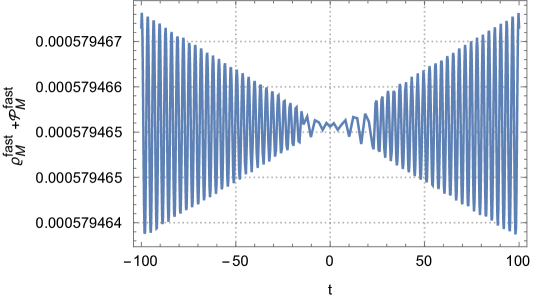
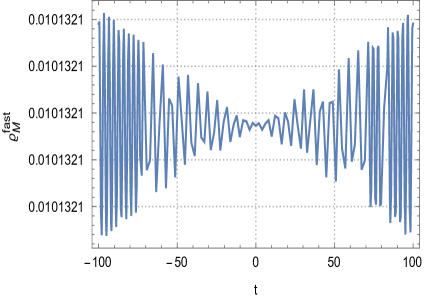
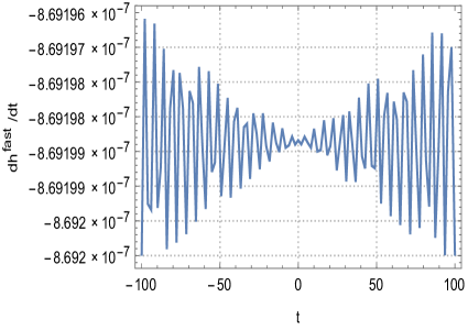
In microscopic time of unit , we numerically solve non-linearly coupled Eqs. (3.4) and (3.9-3.11) with the initial condition (3.12). We report the results in Fig. 1 and details in Fig. 11 of Appendix. Similar to the previous results [41], we find that in the quantum period of microscopic time , the negative quantum pressure and back-reaction effects lead to the quantum pair oscillation in a time characterised by the frequency . The small varies around at . The massive pairs’ density and pressure () oscillate coherently with the spacetime fields oscillations. Their oscillatory structures imply a quantum back-and-forth process in microscopic time scale
| (3.13) |
between spacetime fields and massive particle pairs , previously discussed [39]. These results show the highly non-adiabatic and complex nature of massive pair-production processes and collective oscillations. Attributed to complex back-and-forth reactions at the scale , the quantum massive pair oscillation (3.13) cannot be described by oscillating scalar fields with polynomial potential.
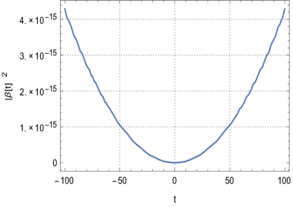
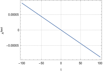
As shown in Figs. 1 and 11, for the microscopic time , the positive quantum pair density indicates particle creations without suppression. It is consistent with increasing Bogoliubov coefficient that mixes positive and negative energy modes. Observe that and the sum is positive definite, leading to the decreasing (3.11). As a consequence, for positive time () increasing (forward the future), the fast components and decrease, in order for pair production. Whereas for negative time () increasing (backward the past), and increases, due to pair annihilation. In both situations, the is negative and is positive, as required by the energy conservation (3.11) in the massive pairs’ production via fast oscillating and . Equations imply the dark energy decreases and matter increases, where the slow components are fixed values at . In this sense, dark energy converts to massive pairs (matter) in a microscopic time scale, whereas the case for a macroscopic time scale will be studied in Sec. 5. It is our finding that the energy density and pressure (3.9,3.10) of the condensate state coherently interacts and exchanges energy with the fast components of spacetime variation (3.11). Such the back-and-forth reaction at the scale was not studied in Ref. [23] for the condensate state’s energy density (3.8) and pressure (3.7). In our solutions, we find the quantum pressure and its time average are negative see Fig. 11 in Appendix. It implies the possibility that the condensate state retains while it coherently interacts with the fast components of spacetime horizon variation (3.13).
This phenomenon is dynamically analogous to the plasma oscillation of electron-positron pair production in an external alternating electric field [44]. The pair production rate is not exponentially suppressed by [45]. The coherent plasma state of electron-positron pairs is analogous to the coherent pair state (3.6) and quantum pair oscillation, shown in Fig. 1.
Such massive and semi-classical state of large occupation number (3.6) and quantum pair oscillation (Fig. 1) well localises inside the horizon. They persist throughout the entire Universe’s history, independent of slow components and values in Friedman equations (2.2,2.3). However, the pair mass (oscillating frequency ) and pair number depend on slow components’ values in the Friedman equations (2.2,2.3). It is necessary and deserves to proceed with further studies.
4 Massive pair plasma state and holographic hypothesis
4.1 Reasons for a macroscopic description
We see the non-adiabatic and back-reacting phenomena of massive pairs’ production and oscillation at a time scale . How the fast oscillating components (3.9) and (3.10) in Eqs. (2.4,2.5) couple to the slow components in Friedman equations (2.2,2.3). It is a difficult task to simultaneously analyze and back-reaction dynamics even numerically since two scales are very different. To deal with this difficulty, we adopt two approximate steps. First, due to nontrivial time-averaged values of fast components over the microscopic time , we assume the massive pair production and oscillation form a massive pair plasma state in the macroscopic time scale. We model such a semi-classical state as a perfect fluid by defining the effective density and pressure. Second, we discuss how it back-and-forth interacts and contributes to the slow components in the Friedman equations.
Figure 1 shows that massive pair quantum pressure (3.9) and density (3.9) rapidly oscillate with the fast components and (3.11) in microscopic time. Their oscillating amplitudes are significantly large and not dampening in time. It, therefore, expects to form a massive pair plasma state in a macroscopic time and space. However, to study its effective impacts on the classical Friedman equations (2.3), we have to discuss two problems stemming from the scale difference .
-
(i)
First, the different time scales. It is impossible to even numerically integrate slow and fast component coupled equations (2.3,2.5) due to their vastly different time scales. On this aspect, we consider the fast-component averages over the microscopic time scale. Figure 1 shows , which does not oscillate alternatively between negative and positive values. Its time average does not vanish. Other fast-component averages do not vanish as well. Fast-component averages have another time scale (5.1) in response to the slow horizon variations in macroscopic time. It is a kind of “relaxation” time scale and differs from the oscillating one . Therefore, in principle, fast-component averages possibly affect the Friedman equation at the macroscopic time scale. In practice, the appropriate modelling of fast-component averages can avoid the difficulty of vastly different scale dynamics in calculations, and the scenario becomes tractable. However, we have to check its self-consistency with observation.
-
(ii)
Second, the spatial distribution. We do not know the spatial distribution of the massive pair condensate state . Namely, we do not know the radial dependence of the quantum pressure and density (3.7,3.8) or (3.9,3.10), since the Ref. [23] authors obtained them by using the vacuum expectation value of field (3.1) energy-momentum tensor integrated over the entire space. There, they studied the cosmic singularity problem in the Universe beginning case, namely the massive mode wavelength is comparable with the horizon size . Here, we study the case , namely the massive mode wavelength is much smaller than the horizon size . As a hypothesis, we speculate that the massive pair condensate state and the coherent oscillation (3.13) with and spatially localize nearby the horizon following the holographic principle [46, 47, 48]. The arguments are the following. (a) Such condensate state and oscillation (3.13) collectively couple with the fast components and , which are quantum modes at short wavelengths (). These modes should associate with the horizon surface according to the holographic principle. (b) The massive pair condensate state is a ground state of a spherically symmetric wave. (c) Such a very massive state of the radial size about is inside the horizon of the Friedman Universe, whose isotropic homogeneity extends up to the horizon.
Based on these hypotheses, we will introduce a holographic and massive pair plasma state that gives an effective description of the condensate state and coherent oscillation (3.13) at macroscopic space and time scales.
4.2 Effective description of a massive pair plasma state
Based on these considerations, we assume a massive pair plasma state forms in a macroscopic time scale. We describe such macroscopic state as a perfect fluid state of effective number and energy densities 555Here we present the simplest state, and it can be a more complex state of massive pair plasma.
| (4.1) |
and pressure . The for and its upper limit is . The introduced mass parameter represents possible particle masses , degeneracies and the mixing coefficient (3.5). The degeneracies plays the same role of pair number in Eqs. (3.7,3.8) or (3.9,3.10). The pair masses are smaller than the Planck mass , but the mass parameter can be larger than for a large occupation number or degeneracy . Note that the massive pair plasma state contains (i) unstable massive pairs that couple and decay to light particles; (ii) stable massive pairs with gravitational interaction only. Besides, one should differ the massive pair plasma state density (4.1) from the normal matter or radiation (including dark matter) density . The reason is that the massive pair plasma state (4.1) attributes to quantum pair production and oscillation, which couple to the oscillating spacetime fields of Hubble function and dark energy. To some extent, we may consider the massive pair plasma state as an “equilibrium state” between quantum massive pairs and spacetime field oscillations.
Following the previous subsection discussions, we explain the reasons why the densities (4.1) are proportional to , rather than of the entire Hubble volume . The “surface area” factor is attributed to the spherical symmetry of Hubble volume. The “radial size” factor is the layer width introduced as an effective parameter to describe the properties: (i) for the massive pair plasma state localizes as a spherical layer near to the horizon; (ii) the layer radial width depends on the massive pair plasma oscillation dynamics 666It may also include self-gravitating dynamics due to the pair plasma state being very massive., rather than the dynamics govern by the Friedman equations (2.3). The width parameter expresses the layer width ,
| (4.2) |
Note that studying the prescription of high-energy modes’ subtraction for , we approximately obtained the mean density (4.1) and by studying massive fermion pair productions in a De Sitter spacetime of constant and scaling factor [39, 40]. We adopt this value for numerical calculations in the present article.
Since the parameters and represent time-averaged values over fast time oscillations of massive pair plasma state, we consider and as approximate constants in slowly varying macroscopic time for the Friedman equations. However, the typical and values should be different for Universe evolution epochs since the fast-component equations for massive pair productions and oscillations depend on the value, see Sec. 3. We used the parameter for inflation, for reheating and for the epochs after reheating. We will fix these parameter values by observations.
To end this section, we have to point out that (i) the pressure and density (4.1) are effective descriptions of the massive pair plasma state in macroscopic scales, that result from the coherence condensation state (3.6,3.7,3.8) and oscillating dynamics (Fig. 1) in microscopic scales; (ii) they contribute to the “slow” components and in the “macroscopic” Friedman equations (2.2,2.3). It means that in the Friedman equations (2.2,2.3), the matter density and pressure terms and contain (a) the normal matter state contributions and (b) the massive pair plasma state contributions. This will be clarified in the next Section. We shall study the massive pair plasma state effects on each epoch of the Universe’s evolution. Here we investigate its impact on reheating.
After we adopt the effective description of massive pair plasma state (4.1), the quantum massive pair oscillation (Fig. 1) of fast components and details at the scale average out and become irrelevant for the macroscopic scale and processes: inflation, reheating and standard cosmology. The relevant quantities and equations are massive pair plasma state (4.1) and slow components obeying Friedman equations (2.2,2.3), and their interacting equation (5.5). The final results depend only on the plasma state (4.1) with the mass and width parameters. Henceforth we ignore the “fast” components, sub-script, and super-scripts “slow” will be dropped.
5 Back-and-forth process and cosmic rate equation
In Sec. 3, we show massive pairs’ production and annihilation at time scale via quantum pair oscillations, and dark energy effectively converts to massive pairs for the microscopic time . These are the quantum back-and-forth process (3.13). By non-vanishing averages over microscopic time, these microscopic back-reaction processes should impact the classical and slow components in Friedman’s equations. Using massive pair plasma state (4.1), we will discuss how to effectively describe the back-and-forth process between massive pairs and spacetime fields at a macroscopic time scale .
5.1 Stable massive pairs and cosmic rate equation
We discuss here how the massive pair plasma state (4.1) back-reacts and contributes to the slow components in Friedman equations. First, we introduce the mean pair production rate to describe the massive pair plasma state variation as the macroscopic time varies. We estimate the total number of particles produced inside the Hubble sphere and mean pair production rate w.r.t. macroscopic time variation ,
| (5.1) |
It is in terms of the parameter (4.2) and Universe evolution -rate defined as,
| (5.2) |
The second equation comes from the Friedman equations (2.2,2.3). The asymptotic values , and correspond to the dark-energy (inflation), radiation, and matter dominant epochs, respectively.
The massive pair plasma state (4.1) effectively represents an equilibrium state of quantum pair and spacetime field oscillations (3.13). It not only depends on the Hubble function , but also contributes to the normal matter density . Back reactions must act on , when and vary in time following the Friedman equations. Moreover, the massive pair plasma state variation time scale is smaller than the normal matter density 777For the sake of brief notation, stands for in this section variation time scale . The difference implies the back-and-forth interaction between the massive pair plasma state density and the normal matter density
| (5.3) |
during the Universe’s evolution. The process is induced by quantum pair oscillation coherently with fast oscillating components of the Hubble function and dark energy.
To model such dynamics (5.3), we recall the rate equation for the back-and-forth process [49, 50, 51, 52]:
| (5.4) |
where is the electron and positron pair density governed by the macroscopic time scale evolution. While is the density of electrons and positrons in equilibrium with two photons in microscopic time scale , namely . The RHS represents the averaged interacting rate for microscopic detail balance between and . They are coupled for and decoupled for .
We make the following analogies: , and photons correspond to fast oscillating components of the Hubble function and dark energy. This analogy motivates us to propose an effective cosmic rate equation
| (5.5) |
of the Boltzmann type for the the back-and-forth and interaction (5.3) in the Universe’s evolution. It represents a general conservation law of dark energy and matter, including massive pair plasma state (4.1) with the production rate (5.1). The term of the time scale represents the space-time expanding effect on the density . While is the source term and is the depletion term. The detailed balance term indicates how two densities and of different time scales couple together. The ratio indicates the coupled case, and indicates the decoupled case. The last term represents unstable massive pairs’ decay to relativistic particle pairs , and the decay rate and time are given by
| (5.6) |
where is the Yukawa coupling between the massive pairs () and relativistic particles. It is important to note that the decay rate (5.6) depends not only on the Yukawa coupling but also on the phase space of final states. While for stable massive pairs, the decay rate is zero.
The combination of cosmic rate equation (5.5) and Friedman equations (2.3) yields
| (5.7) | |||||
| (5.8) |
where , representing the interaction and exchange between dark energy and normal matter via the massive pair plasma state . To discuss this in some more detail, we ignore the decay term . It is negligible for unstable pairs, provided . We point out four particular cases:
-
(i)
Recall the results [41] for the inflation epoch, when the radio , and 888In Ref. [41], we approximately neglect and cosmic rate equation (5.5) to obtain an analytical solution.. Equations (5.7,5.8) become showing production costs dark energy, but it adds into matter-energy . The exchange rate is positive and small. It yields and , i.e., slow-rolling dynamics for inflation. Dark energy converts slowly to matter till inflation ends when .
-
(ii)
In a short pre-reheating episode, when and , the exchange rate is large. Dark energy rapidly converts to matter till . The conversion is very efficient. Details will be in Sec. 7.1.
-
(iii)
The coupled case is and , when tightly couples with in the Universe evolution of the Hubble time scale . Dark energy and matter exchange rate is very small. Dark energy is almost constant in time . It is the case for the matter-dominated episode in reheating, see Sec. 7.2, and for stable massive pairs (cold dark matter) evolution, see Sec. 9.
-
(iv)
In case (iii), has two possibilities: (a) and , dark energy slowly converts to matter ; (b) and , matter slowly converts to dark energy . The (b) is the case for epochs after reheating. Dark energy converts to matter and reduces to its minimal value in reheating, and matter and radiation become dominant over (much larger than) dark energy. However, dark energy weakly couples to matter and radiation, i.e., and . Its variation is much more slowly than matter/radiation decrease. Then it dominates over matter and radiation today. We present the preliminary discussions in Ref. [53].
The inclusion of decay terms and transitions from one case to another are complex and need numerical studies.
5.2 Unstable massive pair decay and reheating equation
Coming from massive unstable pairs’ decay, the radiation energy density of relativistic particles (5.6) obeys the energy conservation law, see for example Ref. [49],
| (5.9) | |||||
where is the massive pair energy, that converts to radiation energy. It leads to the reheating equation
| (5.10) |
As a result, we have a close set of four ordinary differential equations to uniquely determine the time evolution of the Hubble rate , dark-energy density , massive particles’ energy density and relativistic particles’ energy density . They are generalised Friedman equations (2.2,2.3) for and , the cosmic rate equation (5.5) for , and the reheating equation (5.10) for . In addition, there are four algebraic relations: the massive pair plasma density (4.1), the pair-production rate (5.1), the Universe evolution -rate (5.2) and the pair-decay rate (5.6). We will numerically solve these equations, provided initial conditions are known.
6 Initial conditions and basic equations for reheating
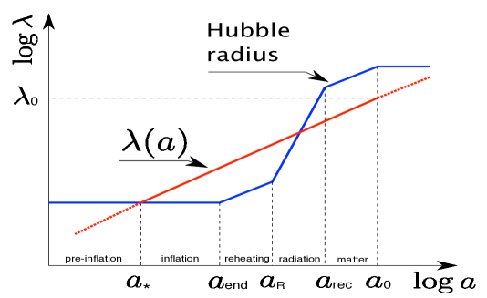
The inflation epoch () ends, and the reheating epoch () starts. The transitioning process must be very complex due to the back reactions of microscopic and macroscopic processes. We assume the transition to be instantaneous at the inflation end and when . For the inflation epoch from to , see Figure 2, we obtain [41]
| (6.1) |
where the inflation scale and correspond to the pivot scale crossed the horizon for CMB observations [55]. The observed spectral index and scalar amplitude determine and the of the -rate (5.2) in inflation. The -folding number and the tensor-to-scalar ratio are related by
| (6.2) |
and implies . The observational constraint on the tensor-to-scalar ratio and spectra index , see Fig. 2 of Ref. [41], gives . The small variation implies at the inflation end
| (6.3) |
and . We approximately adopt the value
| (6.4) |
for which . These are the reheating epoch initial conditions.
Using the characteristic scale and density , we normalize ,
| (6.5) |
Here we introduce the mass parameter or as a typical scale parameter for reheating and will fix its value by observations. Thus, we recast the Friedman equations (2.2) and (2.3), the cosmic rate equation (5.5) and reheating equation (5.10) as,
| (6.6) | |||||
| (6.7) | |||||
| (6.8) | |||||
| (6.9) |
The ratios are
| (6.10) |
and the -rate (5.2) becomes
| (6.11) |
Instead of the cosmic time , here we adopt the cosmic -folding variable and for the sake of simplicity and significance in physics. In the next sections, we will numerically integrate these basic equations (6.6-6.11) for the reheating epoch by using the inflation end (6.4) as the initial condition.
We have to emphasize that the differential equations (6.6-6.9) represent a macroscopic back-and-forth reaction system characterized by the scales , and . It describes the processes: inflation, reheating and standard cosmology. It differs from the differential equations (2.4-2.5) and those in Sec. 3 for a microscopic back-and-forth reaction system of fast-oscillating components characterized by the scale . The fast components’ contributions are effectively represented by the massive pair plasma state (4.1) that enters the cosmic rate equation (6.8).
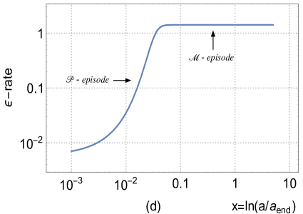
7 Different episodes in reheating epoch
In the reheating epoch, generally speaking, the horizon and the dark energy decreases, as the matter content or increases, meanwhile the ratio (6.10) and the -rate (6.11) increase. To gain insight into the physics first, we use the -rate values (6.11) to characterize the different episodes in the reheating epoch. In each episode, the rate slowly varies in time, we approximately have the time scale of the spacetime expansion . In the transition from one episode to another, the -rate significantly changes its value. Using the characteristic values , we identify the following three different episodes -episode, -episode and -episode in the reheating epoch.
7.1 Preheating -episode: dark energy converting into matter
The short preheating -episode is the transition from the inflation end to the reheating start. In this episode, the pair production rate (5.1) is larger than the Hubble rate , that is still much larger than the pair decay rate (5.6),
| (7.1) |
The radiation energy density is completely negligible . We neglect massive pairs decay to light particles (5.6). The reheating equation (6.9) is then not relevant, and the basic equations (6.6), (6.7) and (6.8) reduce to
| (7.2) | |||||
| (7.3) | |||||
| (7.4) |
where the ratio (6.10) increases as the -rate (6.11)
| (7.5) |
In the -episode, these equations uniquely determine the evolution of the Hubble rate , pairs’ energy densities and dark-energy density .


7.1.1 High efficiency of dark energy converting into matter
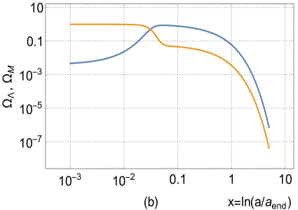
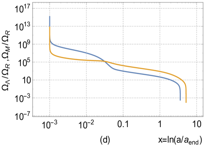
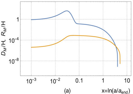
Using the values (6.1) and (6.4) at the inflation end as the initial conditions for the -episode, we numerically integrate Eqs. (6.6), (6.7) and (6.8), by selecting values of the mass parameter . In Figs. 3 and 4, the numerical solutions are plotted in terms of the -folding variable . These solutions show an important result that the dark-energy density is significantly converted to the matter-energy density , as the pair-production rate increases and becomes much larger than the Hubble rate . In more detail, we list that in the -episode the physical quantities vary in time as follows,
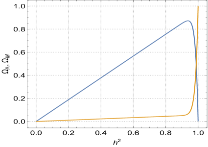

In Figure 4 (left), we plot the energy densities and as functions of the horizon , corresponding to Figures (a) and (b) in Fig. 3. It shows two branches of asymptotic solutions (orange) respectively,
| (7.6) |
and the turning point is about , at which exceeds and the rapid converting process takes place. The characteristic behaviour (7.6) is the same as that in the pre-inflation and inflation epochs. Correspondingly, two branches of asymptotic solutions for the matter (blue) are
| (7.7) |
and , where when . The coefficients and in Eqs. (7.6) and (7.7) can be numerically obtained. As and increases, , and .
Figure 4 (right) shows that in the preheating -episode, the dark energy density converts to the matter-energy . The ratio rapidly increases in a few -folding numbers from at the inflation end to a value . Then becomes dominant. The Hubble rate rapidly decreases and becomes much smaller than the pair-production rate . We define the -episode end at by from Figs. 3 and 4 (right). It shows that the preheating -episode is a very brief transition episode.
We ought to discuss the condition for high efficiency of dark energy converting into massive pairs’ energy in this preheating -episode. Figure 3 (b) shows decreases and increases rapidly, the efficiency of dark energy converting matter-energy is large. The reasons are the following. (i) The ratio increases rapidly as decreases rapidly, see Fig. 3 (c) and (a), respectively. (ii) The rate (5.2) rapidly increases to the order of unity, see Fig. 3 (d). (iii) The mass parameter (5.1) is large, see Fig. 4 (right), which implies heavy mass and large number of pairs produced in the massive pair plasma state (4.1). If the mass parameter is small, the dark energy and matter conversion efficiency is small, see the ratio in Fig. 4 (right). A priori, we do not have theoretical arguments about how much value is. Instead, we select values a posteriori in comparison with observations, and the Universe does not stay cold state of . The necessary condition is the existence of a threshold for which of efficient conversion in reheating.
7.1.2 Threshold of massive pair mass and number for
Figure 4 (right) shows an important result. These solutions depend on the pair mass parameter (4.1) introduced for the reheating epoch. There exists a theoretical threshold on the mass parameter .
-
(a)
For large mass parameters , the pair energy density exceeds the dark-energy density and the asymptotic value ,
(7.8) The reason is that the number (or effective degeneracy ) of massive pairs produced in the reheating epoch has to be large enough so that and the conversion from to is efficient. It corresponds to the physical situation that the most radiation and matter of the Universe is generated in the reheating epoch.
-
(b)
For small mass parameters , the massive pairs’ energy density never exceeds the dark-energy density , namely . The conversion from to is inefficient. This case corresponds to the unrealistic situation that the Universe inflation would never have completely ended, i.e., the cosmological term always dominates .
Observe that the mass parameter of the reheating epoch is larger than the mass parameter of the inflation epoch. From the viewpoint of pair production, the pair mass scale in reheating should be smaller than that in inflation since the reheating horizon is smaller than the inflation one. Therefore, it implies that the effective numbers of massive pairs produced in reheating, is much larger than that of massive pairs produced in inflation . These massive pairs contain both stable and unstable pairs.
Equation (7.5) shows that the asymptotic value of the Horizon variation -rate (5.2) relates to the ratio asymptotic value, see Figs. 3 (d) and 4 (right). For large mass parameter , the ratio 999This condition also admits the possibility of a small negative dark energy density and . Namely, Figure 3 (b) admits solution and drops slightly below zero., the -rate (7.5) approaches to the asymptotic value . It shows the episode of massive pairs domination: -episode.
7.1.3 Minimal comoving radius location
Before discussing the -episode, we would like to mention the turning point at which the Universe acceleration vanishes ,
| (7.9) |
which is obtained from the component of the Einstein equation
| (7.10) |
At this turning point, the Universe stops acceleration and starts deceleration . The turning point occurs at for and . It tells us the balance point of the competition between and in the -episode.
On the other hand, the minimal value of the comoving radius locates at
| (7.11) |
From Friedman equations (2.1), we obtain
| (7.12) |
coinciding with the turning point (7.9). Namely at the minimal comoving radius , the Universe stops acceleration and begins deceleration , starting the reheating epoch and standard cosmology. This is indeed the case for large mass parameter and the ratio becomes larger than 2. The numerical results (Fig. 3) show that this turning/minimal point locates at and .
While the turning/minimal point is never reached, for the cases of the small mass parameter and the ratio is always smaller than 2, see Fig. 4 (right). The reason is that dark energy converting to matter is inefficient, the massive pairs energy is not large enough to balance the dark energy and slow down the Universe’s acceleration. The Universe keeps acceleration and does not run into the reheating epoch. Therefore, the mass parameter range below the threshold (7.8) should be excluded.
7.2 Massive pairs domination: -episode
After the -episode transition, it is the -episode of massive pair domination characterised by
| (7.13) |
The radiation energy density is negligible in the basic equations (6.6-6.11). The variation -rate in Fig. 3 (d) for in Fig. 4 (right). In this episode, the Hubble rate and scale factor vary as
| (7.14) |
and the pair energy density .

Moreover, the back-and-forth processes (5.3) are important, as described by the cosmic rate equation (7.4) with the detailed balance term ,
| (7.15) |
and we define its characteristic time scale
| (7.16) |
Note that differs from (5.1). The microscopic time scale is much smaller than the macroscopic expansion time scale , . Therefore, the back-and-forth (5.3) can build an energy equipartition , and the detailed balance term (7.15) vanish in its time-averaged
| (7.17) |
over the macroscopic time . The cosmic rate equation becomes approximately
| (7.18) |
whose solution is . It is consistent with the matter-dominated solution to Eq. (2.3), yielding . It is also self-consistent with the pair plasma density (4.1) .
In order to verify these discussions and , we check the solution (7.17) or (7.18) analytically and numerically. The averaged over the time consistently obeys the same equation (7.18) for ,
| (7.19) |
where . Numerical results quantitatively show the same conclusion , see Fig. 5 (a), and the detailed balance term (7.15) vanishes, see Fig. 5 (b). Thus we conclude that in the -episode, due to and , the massive pairs plasma state tightly couples with the mass density in the evolution.

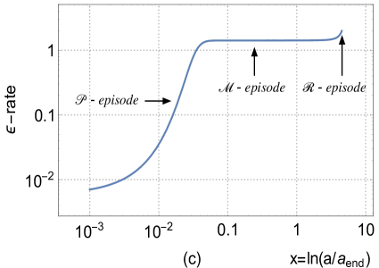
7.3 Relativistic particles domination: -episode of genuine reheating
At the end of the -episode, the massive pairs’ decay term in equations (6.8,6.9) starts to dominate, when the time . The (5.6) is the characteristic time scale of massive pairs decay to relativistic particles. It represents the reheating period of producing tremendous amounts of entropy. The reheating epoch starts its genuine reheating episode, i.e., -episode.
7.3.1 Massive and unstable pairs decay to relativistic particles
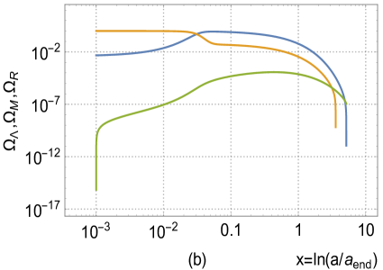
To study the -episode, we numerically solve the closed set of the basic equations (6.6-6.9) with the radiation energy density and the decay term,
| (7.20) |
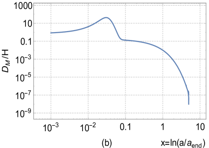
and we define the characteristic time scale of the decay term , which is the same as (5.6). The initial condition of the radiation energy density is at the inflation end , in addition to the initial conditions (6.1) and (6.4). We report the numerical results in Figures 6. It shows that in the (6.6), the radiation energy density increases and becomes dominant, compared with and .
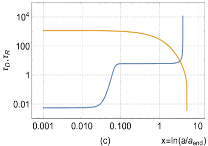
We explain this phenomenon by comparing the decay term (7.20) with the detailed balance term (7.15) in the cosmic rate equation (6.8). Two different dynamics and compete with each other in the process. The is negligible when , while the is dominant when , and the transition from one to another occurs approximately at , where , as shown in Figs. 7 (a) and (b). More precisely, it is the comparison between the characteristic time scale (7.16) of the back-and-forth process (5.3) and the characteristic time scale (7.20) of the pair decay process (5.6). When , the faster back-and-forth process (5.3) dominates, whereas , the faster decay process (7.21) dominates.
In Figs. 7 (c) and (d), two-time scales and are plotted as dimensionless quantities and to show two episodes:
- (i)
- (ii)
The separatrix of two episodes locates at (), i.e., the crossing point of blue and orange lines in Figs. 7. It roughly gives the value at which the genuine reheating occurs.
The value decreases as the Yukawa coupling increases, shown by the left column (a,c) and the right column (b,d) of Figs. 7. Around this point , Figures 6 (b) and (d) show , and Fig. 6 (c) shows , indicating the radiation domination. At , the numerical calculations of the equations (6.6-6.9) run into the stiffness system of step size being effective zero. However, the analytical solution to these basic equations is studied in the next section.


7.3.2 Energy densities of massive pairs and relativistic particles
The -episode is characterised by
| (7.21) |
and , as shown in Figs. 6. As a result, Equations (6.6) and (6.7) or Eq. (6.11) give
| (7.22) |
Following the line presented in Ref. [49], we discuss how the massive pairs transfer their mass energy to relativistic particles, and calculate the radiation energy density , entropy and temperature of relativistic particles.
Since unstable massive pairs predominately decay to relativistic particles, the detailed balance term (7.15) is negligible, and the cosmic rate equation (6.8) reduces to,
| (7.23) | |||||
| (7.24) |
The reheating equation (6.9) becomes
| (7.25) |
In theory, it requires the the time integration from the initial time when to the final time to obtain the radiation energy density ,
| (7.26) |
Through their gauge and other induced interactions, these relativistic particles including sterile particles and other particles beyond the SM interact with each other. They are quickly thermalised at a very high temperature , due to their high number and energy densities. The local thermalisation time scale is much shorter than the expansion time scale , and thus the local thermal equilibrium is built.
7.3.3 Reheating temperature and entropy
We follow the approach [49] to calculate the reheating temperature and entropy. The second law of thermodynamics applied to a comoving volume element yields
| (7.27) |
where is the pair mass energy and is the entropy of relativistic particles produced from massive pairs decay. Therefore, in a comoving volume, the entropy and energy densities of relativistic particles at the thermal state of temperature are given by,
| (7.28) |
The appropriately time-averaged degeneracy over the decay period counts for the total number of effectively massless degrees of freedom, those species share a common temperature . Using the entropy (7.28), one writes Eq. (7.27) as,
| (7.29) |
Integrating this equation over the decay period from the initial scale factor to the reheating scaling factor leads to an approximate solution
| (7.30) |
Here one adopts Eq. (7.24) and , namely, the initial massive pairs’ entropy is approximately zero. In principle, it requires integrating from the initial time to the final time , when the entropy significantly increases. In practice, and are approximately adopted in Eq. (7.30), since the all-important entropy mainly produces in the reheating period .
At the scale factor , the reheating scale can be obtained by from the Friedmann equation (6.6) or the reheating temperature from the thermalization (7.28) [49]:
| (7.31) | |||||
| (7.32) |
It leads to the reheating temperature
| (7.33) |
and the all-important entropy per comoving volume,
| (7.34) |
Equations (7.31) and (7.32) physically mean that at the the genuine reheating (i) the Hubble rate is in the same order as the pair decay rate; (ii) the radiation energy is predominate. These results depend on the effective degeneracy (7.28) and the decay rate (5.6).
Our numerical calculations show the consistency of the approximation used in Eq. (7.30) and the agreement with the analytical solutions (7.31) and (7.33). From Figs. 6 and 7, we find that the reheating predominately takes place around , at which , and the ratios . Moreover, from Fig. 6 () we obtain the reheating scale
| (7.35) |
for the case and . We also obtain (the plot is not present), and for the case .
To estimate the the scale factor change in the reheating epoch, we approximately use the conservation law (7.18) for the massive pair domination
| (7.36) |
Here the initial pair energy density (6.3) at the beginning of the reheating epoch, and the final one at the end of the reheating epoch, in virtue of Eqs. (7.28) and (7.32).
8 Observations to fix reheating temperature and entropy
We use the method proposed by Ref. [54] to fix the reheating temperature by the CMB observations. The cosmological evolution of the physical wavelength and wavenumber is
| (8.1) |
where the present time , the comoving wavenumber and wavelength are constants in the evolution, see Figure 2. The total increase of the scale factor from the horizon crossing (6.1) to is given by
| (8.2) |
At the CMB pivot scale , the scalar spectrum gives
| (8.3) |
On the other hand, as illustrated in Fig. 2 and Ref. [54], , and are given in terms of the temperature and redshift at the recombination,
| (8.4) |
Whereas, we compute (6.1) and (7.36) in the CDM scenario. As a result, we obtain
| (8.5) |
It agrees with the result (33) using the inflation potential energy density (17) in Ref. [54]. Here we adopt the energy density (6.3) at inflation end.
Equations (8.3) and (8.5) are independent of the effective reheating degeneracy and yield the reheating temperature
| (8.6) |
in terms of the CMB observations eV and ( eV), as well as (6.2) and (6.1), whose values depend on the CMB measurements , and , see Sec. 6.


8.1 Reheating temperature and entropy vs tensor-to-scalar ratio
Given the observed the scalar amplitude and spectral index , the inflation ending -folding number (6.1) and the reheating temperature (8.6) are plotted in Fig. 8 as functions of the tensor-to-scalar ratio without any free parameter. Figure 8 shows that their values are and in the range .


After obtaining the reheating temperature at the end of reheating, we calculate the entropy produced within the physical patch of the volume , which evolves from the initial patch of the volume at the start of the inflation. The patch grows by a scale factor of Eqs. (6.1) and (7.36),
| (8.7) |
The entropy per comoving volume (7.34) at the end of reheating is expressed as
| (8.8) |
where we use (7.36) and the constraint (8.11) below. The entropy within the physical patch is given by,
| (8.9) |
which is a function of and . In Fig. 9 (right), we plot by using (6.2), (6.1) and (7.32). It shows the calculated entropy accords with the observational value around .
To have a better understanding of how the physical patch horizon evolves, we plot in the same Fig. 9 (left) all characteristic Hubble scales from the inflation to the reheating: the inflation scale , inflation end scale (6.1), and reheating scale (7.32) in unit of the Planck scale . It shows that the nonphysical situation occurs when . Therefore the range excludes. Due to the dependence of on and the approximations adopted in these calculations, we conservatively suggest a theoretical upper limit of the tensor-to-scalar ratio . This theoretical upper limit is consistent with the observational one [56], and the recent constraint [57].
In the -range , we show that (i) the inflation -folding number and the reheating temperature from the numerical results presented in Fig. 8; (ii) the inflation scale , inflation end scale , whereas and the entropy from the numerical results presented in Fig. 9. These results show that the CDM scenario is consistent with observations. The precisely measuring -value is essential to determine the -folding number of the inflation, the reheating temperature, all characteristic Hubble scales and produced entropy.
8.2 Genuine reheating and tensor-to-scalar ratio
In the CDM scenario, there are two parameters to describe the properties of the reheating epoch: (i) the effective mass parameter physically represents pairs’ masses and numbers; (ii) the effective Yukawa coupling represents pairs’ decay strength to relativistic particles of degeneracies .
To determine these two parameters, we use Eqs. (7.33) and (8.6) to obtain one constraint,
| (8.10) |
Another constraint is
| (8.11) |
from the reheating temperature (7.33) and the ratio , obtained by the baryon number-to-entropy ratio [58], theoretical relation [49] and , see Eq. (5.3) of Ref. [59].
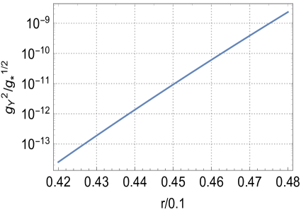
In Fig. 10, we numerically plot the constraints (8.10) and (8.11) as a function of the tensor-to-scalar ratio . Recall that in Sec. 7.1.2 we point out the theoretical threshold : (7.8) for . We conclude that the nontrivial threshold demands the tensor-to-scalar ratio , see also Eq. (6.2). Applying the obtained theoretical threshold to numerical results Fig. 10, we find that the tensor-to-scalar ratio . However, it depends on the parameter adopted and other approximations used for numerical calculations. To obtain the lower limit , it requires more elaborated calculations, for example, separating in Eq. (4.1) unstable modes’ contribution from stable modes’ contribution to more accurately determine the mass parameter threshold . Nevertheless, the obtained -range () is relevant to the measurements by the next generation CMB observations, such as CMB-S4 which measures [60].
We report the numerical results in the range . The effective pair mass parameter is in and the effective Yukawa coupling is in . If for the standard model of particle physics, including sterile neutrinos, the Yukawa coupling is in the range of . We check back the parameters used in Figs. 6 and 7 are and . It indicates that the CDM scenario is self-consistent and self-contained.

9 Stable massive pairs and cold dark matter abundance
To further clarify dark energy and matter interaction, we study stable massive pairs after reheating. These pairs neither decay into light particles nor contribute to reheating. Thus, they remain and can be candidates for massive cold dark matter (CDM) particles. Here, we qualitatively discuss their evolution after reheating.
In the radiation- and matter-dominated epoch after reheating, the Universe evolution rate (5.2) is and , respectively. The mean pair-production rate (5.1) is proportional to the mass parameter . The large mass and ratio imply massive stable pairs should tightly couple with dark energy in evolution. Therefore, we focus on stable pairs interacting with dark energy in Eqs. (5.7,5.8), and approximately obtain
| (9.1) | |||||
| (9.2) |
where indicates the massive pair plasma state (4.1) for stable pairs. For the coupled case , discussed as the case (iii) after Eqs. (5.7,5.8), the approximate solution to Eqs. (9.1,9.2) is
| (9.3) |
| (9.4) |
with approximate solutions and , where indexes [18]. It shows massive cold dark matter approximately follows the evolution of non-relativistic fluid, weakly interacting with dark energy. In other words, via massive pair plasma state , dark energy and cold dark matter interact with each other. However, the exchange between them is small and inefficient. Actually, Eq. (9.3) is essentially the same as Eq. (7.17) and discussions here are similar to the matter-dominated -episode of reheating, see Sec. 7.2. One can also find similar discussions [53] that dark energy weakly interacts with radiation and baryon matter, and their exchange is small and inefficient.
Equation (9.3) indicates the cold dark matter abundance is an approximate constant in time,
| (9.5) |
where . It means that (i) the CDM composes stable massive pairs produced in the pre-reheating -episode, see Sec. 7.1; (ii) the current CDM abundance is approximately equal to its abundance in the -episode (7.2) of reheating, see Sec. 7.2. The approximate constancy of CDM abundance in time is a direct consequence of the holographic and massive pair plasma state (4.1). To be self-consistent, we give a rough check on the magnitude by using the theoretical threshold (7.8) and width parameter constrained by studying inflation [41] and theoretical calculation [39, 40]. It shows the cold dark matter abundance (9.5) can be the right order of the magnitude, compared with the currently observed relic value . This preliminary study requires further detailed investigations. Moreover, as CDM candidates, these massive stable pairs should play some role in primordial black hole formulation and primordial gravitational wave emission.
10 Remarks and summary
10.1 Some remarks
We study the scenario that the cosmological constant term (dark energy) and represents [63, 64, 65, 66, 67, 68] the non-trivial ground state (Wheeler spacetime foam [69]) of the quantum field of spacetime gravity and . Dark energy is neither the vacuum energy of quantum fields of particles (matter) nor the energy of the scalar field’s kinetics and potential. We need further investigations to understand of the spacetime foam interacting to matter. We study in this article the back-and-forth interactions between dark energy and matter via horizon in the following two aspects.
First, at the scale for fast components and their back-and-forth reactions, we describe in Sec. 3 the quantum massive pair production and oscillation. It forms a quasi-classical coherent state with a large occupation number of particles. Averaging fast components over microscopic time, we describe the state as a quasi-classical state of massive pair plasma by using a perfect fluid in Sec. 4. It is functional of dark energy and normal matter via the horizon.
Second, at the scale for slow components and their interactions, we discuss in Sec. 5 the macroscopic back-and-forth interacting system between the classical pair plasma fluid , normal matter fluids , dark energy and horizon via nonlinear Eqs. (6.6-6.9). The novel cosmic rate equation (6.8) accounts for the massive pair plasma state interacting with dark energy and normal matter. The system yields CDM scenario that describes inflation, reheating and standard cosmology.
In Ref. [41], we study -driven inflation in detail, compare and contrast it with usual canonical inflation models of the scalar field , potential , Friedman equation , energy density and pressure . The correspondences between inflation models and the -driven inflation
| (10.1) |
where the dark energy density is an slow component. The fast oscillating component has no relation to the classical field . The slow-roll condition corresponds to for . It leads to and . Equation (2.3), namely Eq. (5.1) in Ref. [41], corresponds to the classical equation of motion for : . In inflation, we approximately obtain an analytical solution by neglecting the cosmic rate equation (5.5) because of . In reheating, we have to numerically solve the Friedman equations, cosmic rate equation and reheating equation (6.6-6.9), which yield a complex back-and-forth reaction system of inter-playing three scales , , and dynamics.
10.2 Summary
We make a summary to close this lengthy article. In the -dominated inflation , where the massive pair plasma density is small and normal matter density is negligible. The reheating epoch starts , and become large, and their back reaction and decay to relativistic particles are important. Therefore, the cosmic rate equation (5.5) governing the processes (5.3) and unstable massive pairs’ decay are relevant. It is an additional dynamical equation to two Friedman equations (2.2,2.3) and the reheating equation (5.10) from energy conservation.
Using the massive pair plasma density (6.5), production rate and decay rate (6.10), we study the reheating epoch by a close system of four dynamical (ordinary differential equations) equations (6.6-6.9) for the horizon and three densities . The initial conditions are given by the inflation end. Numerically solving this system, we find three characteristic episodes:
-
(i)
the -episode of the transition from the inflation end to the reheating start, when the pair-production rate is much larger than the Hubble rate (), the dark energy density quickly decreases and converts to the matter-energy density . As a consequence ;
-
(ii)
the -episode of massive pairs domination, where the back-and-forth interaction of the cosmic rate equation (5.5) plays an essential role, and dark energy density slowly varies;
-
(iii)
the -episode of the genuine reheating , when unstable massive pairs predominately decay to relativistic particles that quickly thermalised.
We emphasise the pair mass threshold (7.8) that at the pre-reheating start , the rapid converting process leads to . The most relevant mass-energy and entropy of Universe are produced by the end of reheating. Such dynamic processes should lead to the emission of primordial gravitational waves [61, 62].
The initial conditions for the reheating epoch are the Hubble scale and energy densities at the end of inflation after -folding number . They are determined by the CMB measurements of scalar amplitude and spectral index at pivot scale and the Hubble scale [41]. We obtain the reheating Hubble scale , temperature and entropy at the genuine reheating episode. They are functions of the tensor-to-scalar ratio , and their numerical values are in accordance with the CMB observations. Moreover, from purely theoretical viewpoints, we preliminarily limit the values in the range . Among massive pairs gravitationally produced, (i) unstable pairs decay to relativistic particles, accounting for reheating; (ii) stable pairs couple only to gravity and are candidates for cold dark matter. The resultant cold dark matter abundance is about a constant in time. They should play the role in the formation of primordial black holes.
11 Acknowledgment
The author thanks the EPJC Editor Alexei Starobinsky and anonymous referees for their reviews and reports that give chances to improve the manuscript.
12 Appendix: Quantum pair oscillation details
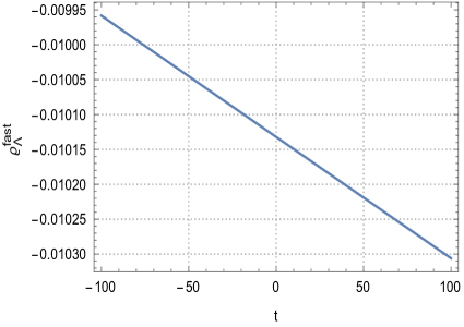
In microscopic time, we plot the Bogoliubov coefficient , the quantum pair density and pressure , as well as the fast components of Hubble function , and cosmological term . Recall .

References
- [1] A. A. Starobinsky, A new type of isotropic cosmological models without singularity, Phys. Lett. B 91 (1980) 99.
- [2] A. H. Guth, The inflationary universe: A possible solution to the horizon and flatness problems, Phys. Rev. D 23 (1981) 347.
- [3] A. D. Linde, A new inflationary universe scenario: A possible solution of the horizon, flatness, homogeneity, isotropy and primordial monopole problems, Phys. Lett. B 108 (1982) 389–393.
- [4] V. F. Mukhanov and G. V. Chibisov, The vacuum energy and large scale structure of the universe, Sov. Phys. JETP 56 (1982) 258–265.
- [5] A. Albrecht and P. J. Steinhardt, Cosmology for grand unified theories with radiatively induced symmetry breaking, Phys. Rev. Lett. 48 (1982) 1220.
- [6] A. D. Linde, Chaotic inflation, Phys. Lett. B 129 (1983) 177.
- [7] R. Kallosh and A. Linde, BICEP/Keck and cosmological attractors, JCAP 12 (2021) 008 [2110.10902].
- [8] L. Kofman, A. D. Linde and A. A. Starobinsky, Reheating after inflation, Phys. Rev. Lett. 73 (1994) 3195 [hep-th/9405187].
- [9] L. Kofman, A. D. Linde and A. A. Starobinsky, Towards the theory of reheating after inflation, Phys. Rev. D 56 (1997) 3258 [hep-ph/9704452].
- [10] Y. Shtanov, J. H. Traschen and R. H. Brandenberger, Universe reheating after inflation, Phys. Rev. D 51 (1995) 5438 [hep-ph/9407247].
- [11] B. A. Bassett and S. Liberati, Geometric reheating after inflation, Phys. Rev. D 58 (1998) 021302 [hep-ph/9709417].
- [12] S. Tsujikawa, K.-I. Maeda and T. Torii, Resonant particle production with nonminimally coupled scalar fields in preheating after inflation, Phys. Rev. D 60 (1999) 063515 [hep-ph/9901306].
- [13] D. I. Podolsky and A. A. Starobinsky, Chaotic reheating, Grav. Cosmol. Suppl. 8N1 (2002) 13 [astro-ph/0204327].
- [14] R. Allahverdi, R. Brandenberger, F.-Y. Cyr-Racine and A. Mazumdar, Reheating in inflationary cosmology: Theory and applications, Ann. Rev. Nucl. Part. Sci. 60 (2010) 27 [1001.2600].
- [15] M. A. Amin, R. Easther, H. Finkel, R. Flauger and M. P. Hertzberg, Oscillons after inflation, Phys. Rev. Lett. 108 (2012) 241302 [1106.3335].
- [16] M. A. Amin, M. P. Hertzberg, D. I. Kaiser and J. Karouby, Nonperturbative dynamics of reheating after inflation: A review, Int. J. Mod. Phys. D 24 (2014) 1530003 [1410.3808].
- [17] P. Adshead, J. T. Giblin, M. Pieroni and Z. J. Weiner, Constraining axion inflation with gravitational waves across 29 decades in frequency, Phys. Rev. Lett. 124 (2020) 171301 [1909.12843].
- [18] S.-S. Xue, How universe evolves with cosmological and gravitational constants, Nucl. Phys. B 897 (2015) 326 [1410.6152].
- [19] L. Parker, Particle creation in expanding universes, Phys. Rev. Lett. 21 (1968) 562.
- [20] L. Parker, Quantized fields and particle creation in expanding universes. II, Phys. Rev. D 3 (1971) 346.
- [21] L. Parker, Quantized fields and particle creation in expanding universes. I, Phys. Rev. 183 (1969) 1057.
- [22] Y. B. Zeldovich and A. A. Starobinsky, Particle production and vacuum polarization in an anisotropic gravitational field, JETP [Zh. Eksp. Teor. Fiz. 61 (1971) 2161-2175] 34 (1972) 1159.
- [23] L. Parker and S. A. Fulling, Quantized matter fields and the avoidance of singularities in general relativity, Phys. Rev. D 7 (1973) 2357.
- [24] V. M. M. S. G. Mamaev and A. A. Starobinsky, Particle production and vacuum polarization in an anisotropic gravitational field, JETP 43 (5) (1976) 823.
- [25] Y. B. Zeldovich and A. A. Starobinsky, Rate of particle production in gravitational fields, JETP Lett. 26, 252-255 (1977) 26 (1977) 252.
- [26] A. A. Starobinsky, Spectrum of relict gravitational radiation and the early state of the universe, JETP Lett. 30 (1979) 682.
- [27] N. D. Birrell and P. C. W. Davies, Quantum Fields in Curved Space, Cambridge Monographs on Mathematical Physics. Cambridge Univ. Press, Cambridge, UK, 2, 1984, 10.1017/CBO9780511622632.
- [28] E. Mottola, Particle creation in De Sitter space, Phys. Rev. D 31 (1985) 754.
- [29] S. Habib, C. Molina-Paris and E. Mottola, Energy momentum tensor of particles created in an expanding universe, Phys. Rev. D 61 (2000) 024010 [gr-qc/9906120].
- [30] P. R. Anderson and E. Mottola, Instability of global De Sitter space to particle creation, Phys. Rev. D 89 (2014) 104038 [1310.0030].
- [31] P. R. Anderson and E. Mottola, Quantum vacuum instability of “eternal” De Sitter space, Phys. Rev. D 89 (2014) 104039 [1310.1963].
- [32] A. Landete, J. Navarro-Salas and F. Torrenti, Adiabatic regularization and particle creation for spin one-half fields, Phys. Rev. D 89 (2014) 044030 [1311.4958].
- [33] A. A. Starobinsky, Nonsingular model of the universe with the quantum-gravitational de sitter stage and its observational consequences, Proc. of the Second Seminar “Quantum Theory of Gravity”,Moscow,October 1981, INR Press, Moscow (1982) 58.
- [34] L. H. Ford, Gravitational particle creation and inflation, Phys. Rev. D 35 (1987) 2955.
- [35] E. W. Kolb, A. D. Linde and A. Riotto, Gut baryogenesis after preheating, Phys. Rev. Lett. 77 (1996) 4290 [hep-ph/9606260].
- [36] D. J. H. Chung, P. Crotty, E. W. Kolb and A. Riotto, On the gravitational production of superheavy dark matter, Phys. Rev. D 64 (2001) 043503 [hep-ph/0104100].
- [37] D. J. H. Chung, E. W. Kolb and A. J. Long, Gravitational production of super-hubble-mass particles: an analytic approach, JHEP 01 (2019) 189 [1812.00211].
- [38] Y. Ema, K. Nakayama and Y. Tang, Production of purely gravitational dark matter, JHEP 09 (2018) 135 [1804.07471].
- [39] S.-S. Xue, Cosmological driven inflation and produced massive particles, 1910.03938.
- [40] S.-S. Xue, Cosmological constant, matter, cosmic inflation and coincidence, Mod. Phys. Lett. A 35 (2020) 2050123 [2004.10859].
- [41] S.-S. Xue, Massive particle pair production and oscillation in Friedman universe: its effect on inflation, Eur. Phys. J. C 83 (2023) 36 [2112.09661].
- [42] D. Bégué, C. Stahl and S.-S. Xue, A model of interacting dark fluids tested with supernovae and baryon acoustic oscillations data, Nucl. Phys. B 940 (2019) 312 [1702.03185].
- [43] L. Parker and S. A. Fulling, Adiabatic regularization of the energy-momentum tensor of a quantized field in homogeneous spaces, Phys. Rev. D 9 (1974) 341.
- [44] Y. Kluger, J. M. Eisenberg, B. Svetitsky, F. Cooper and E. Mottola, Pair production in a strong electric field, Phys. Rev. Lett. 67 (1991) 2427.
- [45] R. Ruffini, G. Vereshchagin and S.-S. Xue, Electron-positron pairs in physics and astrophysics: from heavy nuclei to black holes, Phys. Rept. 487 (2010) 1 [0910.0974].
- [46] G. ’t Hooft, Dimensional reduction in quantum gravity, Conf. Proc. C 930308 (1993) 284 [gr-qc/9310026].
- [47] L. Susskind, The world as a hologram, J. Math. Phys. 36 (1995) 6377 [hep-th/9409089].
- [48] A. G. Cohen, D. B. Kaplan and A. E. Nelson, Effective field theory, black holes, and the cosmological constant, Phys. Rev. Lett. 82 (1999) 4971 [hep-th/9803132].
- [49] E. W. Kolb and M. S. Turner, The Early Universe, vol. 69. 1990, 10.1201/9780429492860.
- [50] B. W. Lee and S. Weinberg, Cosmological lower bound on heavy neutrino masses, Phys. Rev. Lett. 39 (1977) 165.
- [51] R. Ruffini, J. D. Salmonson, J. R. Wilson and S. S. Xue, On the evolution of the pair-electromagnetic pulse of a charged black hole, Astron. Astrophys 138, 511-512 (1999) 138 (1999) 511 [astro-ph/9905021].
- [52] R. Ruffini, J. D. Salmonson, J. R. Wilson and S.-S. Xue, On the pair-electromagnetic pulse from an electromagnetic black hole surrounded by a baryonic remnant, Astron. Astrophys 359, 855-864 (2000) (2000) [astro-ph/0004257].
- [53] S.-S. Xue, Massive particle pair production and oscillation in Friedman universe: dark energy and matter interaction, 2203.11918.
- [54] J. Mielczarek, Reheating temperature from the CMB, Phys. Rev. D 83 (2011) 023502 [1009.2359].
- [55] Planck collaboration, Planck 2018 results. VI. cosmological parameters, Astron. Astrophys. 641 (2020) A6 [1807.06209].
- [56] Planck collaboration, Planck 2018 results. X. constraints on inflation, Astron. Astrophys. 641 (2020) A10 [1807.06211].
- [57] M. Tristram et al., Planck constraints on the tensor-to-scalar ratio, Astron. Astrophys. 647 (2021) A128 [2010.01139].
- [58] Planck collaboration, Planck 2015 results. XIII. cosmological parameters, Astron. Astrophys. 594 (2016) A13 [1502.01589].
- [59] S.-S. Xue, Horizon crossing causes baryogenesis, magnetogenesis and dark-matter acoustic wave, 2007.03464.
- [60] K. Abazajian et al., CMB-S4 science case, reference design, and project plan, 1907.04473.
- [61] M. Maggiore, Gravitational wave experiments and early universe cosmology, Phys. Rept. 331 (2000) 283 [gr-qc/9909001].
- [62] M. C. Guzzetti, N. Bartolo, M. Liguori and S. Matarrese, Gravitational waves from inflation, Riv. Nuovo Cim. 39 (2016) 399 [1605.01615].
- [63] Sidney R. Coleman, Why There Is Nothing Rather Than Something: A Theory of the Cosmological Constant, Nucl. Phys. B 310 (1988) 643–668 [DOI: 10.1016/0550-3213(88)90097-1].
- [64] A. O. Barvinsky, Why there is something rather than nothing (out of everything)?, Phys. Rev. Lett. 99 (2007) 071301 [hep-th/0704.0083].
- [65] S.-S. Xue, Gravitational instanton and cosmological term, Int. J. Mod. Phys. A 24 (2009) 3865–3891 [hep-th/0608220].
- [66] S.-S. Xue, Detailed discussions and calculations of quantum Regge calculus of Einstein-Cartan theory, Phys. Rev. D 82 (2010) 064039 [0912.2435].
- [67] S.-S. Xue, Quantum Regge calculus of Einstein-Cartan theory, Phys. Lett. B 682 (2009) 300 [0902.3407].
- [68] S.-S. Xue, The phase and critical point of quantum Einstein-Cartan gravity, Phys. Lett. B 711 (2012) 404 [1112.1323].
- [69] Charles W. Misner and K. S. Thorne and J. A. Wheeler, Gravitation, 1990, W. H. Freeman publisher, ISBN 978-0-7167-0344-0, 978-0-691-17779-3.