Combination of Tensor Network States and Green’s function Monte Carlo
Abstract
We propose an approach to study the ground state of quantum many-body systems in which Tensor Network States (TNS), specifically Projected Entangled Pair States (PEPS), and Green’s function Monte Carlo (GFMC) are combined. PEPS, by design, encode the area law which governs the scaling of entanglement entropy in quantum systems with short range interactions but are hindered by the high computational complexity scaling with bond dimension (D). GFMC is a highly efficient method, but it usually suffers from the infamous negative sign problem which can be avoided by the fixed node approximation in which a guiding wave function is utilized to modify the sampling process. The trade-off for the absence of negative sign problem is the introduction of systematic error by guiding wave function. In this work, we combine these two methods, PEPS and GFMC, to take advantage of both of them. PEPS are very accurate variational wave functions, while at the same time, only contractions of single-layer tensor network are necessary in GFMC, which reduces the cost substantially. Moreover, energy obtained in GFMC is guaranteed to be variational and lower than the variational energy of the guiding PEPS wave function. Benchmark results of - Heisenberg model on square lattice are provided.
One of the most challenging tasks in condensed matter physics is to understand the many-body effect in strongly correlated quantum systems, in which numerous exotic phenomena emerge Bednorz and Müller (1986); Tsui et al. (1982); Laughlin (1983); Zhou et al. (2017). Because exact solution for strongly correlated system is rare Lieb and Wu (1968), most studies of these systems rely on numerical tools nowadays. Density Matrix Renormalization Group (DMRG) White (1992, 1993) is one of the most successful methods in the study of strongly correlated systems. DMRG is extremely accurate for one-dimensional (1D) quantum systems Schollwöck (2005, 2011). Shortly after the introduction of DMRG in 1992 White (1992), it was realized that the underlying wave functions are Matrix Product States (MPS) Östlund and Rommer (1995), which can be viewed as a generalization of the seminal AKLT state Affleck et al. (1987). The concept of MPS can be traced back at least to 1968 Baxter (1968). It was found that MPS capture the entanglement structure of the ground state of 1D quantum systems and this results in the high accuracy of DMRG Eisert et al. (2010). The adoption of concepts from the field of quantum information, entanglement for example, have inspired the development of the Tensor Network States (TNS) Verstraete et al. (2008). These advances provide us useful tools to both identify Orús (2014) and classify Chen et al. (2011); Schuch et al. (2011) quantum phases.
DMRG can also provide accurate results for systems on narrow cylinders with large enough bond dimension Stoudenmire and White (2012); Yan et al. (2011); LeBlanc et al. (2015); Zheng et al. (2017); Qin et al. (2020) but has difficulty for real 2D system Liang and Pang (1994). A natural generalization of MPS to 2D, Projected Entangled Pair States (PEPS) Verstraete and Cirac (2004), can overcome the difficulty Jiang et al. (2008); Jordan et al. (2008); Corboz et al. (2011, 2014); Liao et al. (2017). It can be proved that the entanglement entropy in PEPS satisfies the area law Verstraete and Cirac (2004) which is required to faithfully represent the ground state of 2D quantum systems Eisert et al. (2010) (when a Fermi surface is present Gioev and Klich (2006), there is a logarithm correction to area law for the ground state, which PEPS fails to capture.). However, in contrast to scaling of complexity in MPS, the computational cost is as high as Jordan et al. (2008); Orús and Vidal (2009); Phien et al. (2015) in PEPS. The heavily scaling of computational resource with bond dimension in PEPS hampers the reach to large bond dimension which is essential to resolve possible competing states in the low energy manifold of certain strongly correlated systems, e.g., the anti-ferromagnetic Heisenberg model on Kagome lattice Ran et al. (2007); Yan et al. (2011); Depenbrock et al. (2012); Iqbal et al. (2013); Liao et al. (2017); Mei et al. (2017).
Quantum Monte Carlo (QMC) Blankenbecler et al. (1981); Orús and Vidal (2009); Assaad and Evertz (2008); Zhang (2004) is a widely used methodology in the study of strongly correlated many-body systems. In general, the computational complexity in QMC scales algebraically with system size which makes it an efficient approach. However, with few exception Orús and Vidal (2009), the direct application of Monte Carlo method in many-body systems suffers from the infamous negative sign problem Loh et al. (1990); Troyer and Wiese (2005). One strategy to overcome the negative sign problem is to take advantage of the trade-off between variance and bias, which is the principle behind fixed node approximation in Green’s function Monte Carlo (GFMC) Kalos (1962); Ceperley and Alder (1980) (also named as diffusion Monte Carlo (DMC) Foulkes et al. (2001) in the literature), and constrained path approximation in auxiliary field quantum Monte Carlo Zhang et al. (1997). The price to pay is the introduction of systematic error or bias in the result. Empirically, different forms of guiding An and van Leeuwen (1991); van Bemmel et al. (1994); Iqbal et al. (2013); Capriotti et al. (1999) or trial wave functions Chang and Zhang (2008); Qin et al. (2016) can be chosen to give high accuracy for certain systems.
In this work, we combine PEPS and GFMC to take advantage of both of them. We take PEPS as guiding wave function in GFMC calculation. As we will discuss late, in our method, only contraction of single-layer tensor network is required, which highly reduces the computational complexity in the PEPS part. At the same time, PEPS are very accurate variational wave functions, with which the systematic error can be reduced in GFMC.
Models – For concreteness, we take the - Heisenberg model on square lattice as an example to describe the method. The Hamiltonian is as follows:
| (1) |
where is the spin operator on site . and represent nearest and next nearest neighboring interactions respectively. We consider anti-ferromagnetic interactions for both and , and set as the energy unit. For simplicity, we study system on square lattice with open boundary conditions (OBC). The - Heisenberg model is widely investigated in the exploration of the frustration effect in quantum systems Chandra and Doucot (1988); Dagotto and Moreo (1989); Capriotti and Sorella (2000). When is absent, the model can be solved with QMC without suffering from the negative sign problem Sandvik (1997); Jiang and Wiese (2011); Sandvik and Evertz (2010). The ground state is known to have the long-range anti-ferromagnetic (AF) order, i.e., the Neel order. In the other limit when , the system decouples into two independent square lattices and an infinitesimal can drive the ground state into the striped AF order. Between these two limits, the nature of the ground state is still under extensive debates Mambrini et al. (2006); Murg et al. (2009); Yu and Kao (2012); Jiang et al. (2012); Mezzacapo (2012); Hu et al. (2013); Gong et al. (2014); Morita et al. (2015); Wang and Sandvik (2018) in the vicinity of where the system is maximally frustrated in the sense that in the classical limit, the - Ising model has macroscopic degenerate ground state.
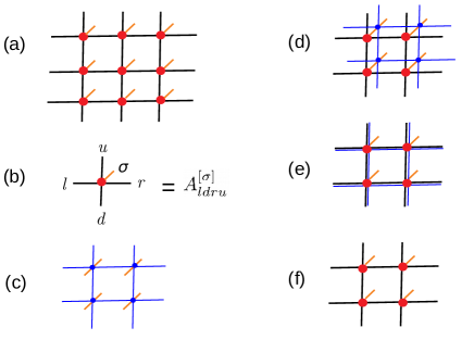
Projected Entangled Pair States – To construct a PEPS, we put a rank five tensor, on each vertex of the square lattice (see Fig. 1 (b)), where is the physical degree of freedom with dimension , while are the auxiliary degree of freedoms with dimension Verstraete and Cirac (2004). Contracting the auxiliary degree of freedoms gives the PEPS wave function
| (2) |
where the trace means contraction of tensors. To obtain the ground state of the Heisenberg model in Eq(1), we apply the imaginary time projection operator repeatedly to an initial PEPS till convergence. Same as in Trotter-Suzuki decomposition Suzuki (1976), we first divide the lattice into four groups of plaquettes in a way that the projection operators of each plaquette within a group are independent or commute with each other. In each group, a Projected Entangled Pair Operator (PEPO) (see Fig. 1 (c)) for the projection operator within a single plaquette is constructed and are applied to the initial PEPS simultaneously. This procedure is carried out recurrently for the four groups (see Fig. 1 (d)). Because the bond dimension increases after the application of PEPO Pirvu et al. (2010) (see Fig. 1 (e)), we need to truncate it back to the original value to make the calculation under-control (see Fig. 1 (f)). This is done in a variational fashion Evenbly (2018), The whole procedure is a realization of the cluster update approach Wang and Verstraete (2011) which is a generalization of simple update Jiang et al. (2008). The most time-consuming part of this approach is the calculation of physical quantities after the PEPS are optimized, which requires contraction of double-layer tensor networks with bond-dimension . As we will discuss late, when combining PEPS with GFMC, we only need to calculate single-layer tensor networks with bond-dimension , which reduces the complexity substantially. We notice the existence of single-layer like algorithm in the literature Xie et al. (2017). In more sophisticated full update scheme of PEPS, the contraction of double-layer tensor network is also needed in the optimization process Jordan et al. (2008); Corboz et al. (2010).
Green’s function Monte Carlo – In Green’s function Monte Carlo Carlson (1989); Trivedi and Ceperley (1989, 1990); Runge (1992), the ground state of a system is also obtained by imaginary time projection . The projection length, , is then divided into small slices with and a small number. In GFMC, we take the first order expansion of the exponential function: with (or ) a positive real number large enough to ensure all the diagonal elements of are positive. Then the ground state can formally be written as with . Mixed estimate is employed in GFMC to calculate the ground state energy as , which gives the exact ground state energy if is the true ground state of . Here we introduce a guiding wave function whose effect will be discussed late. We use to denote spin configuration of the whole system, i.e., , which is also walker in the sampling process. We define the kernel as with and . Then the ground state energy from mixed estimate is
| (3) |
where the local energy is defined as By introducing , we have
| (4) |
So we can view as probability density (if is non-negative) and take advantage of Monte Carlo techniques, metropolis for example, to evaluate the summation in Eq. (4). It is easy to show where the summation is over .
The procedure of GFMC can be summarized as follows. At the first step, we sample according to , and set the weight of each walker to . This gives us an ensemble of walkers . We usually choose and sample with probability . Then each walker is propagated to with probability , where the normalization factor is . After a new walker is chosen, we update the weight of it by multiplying the normalization factor as . This process is repeated and we can start the measurement of energy after equilibrium is reached.
When the off-diagonal elements of the are all non-positive, the ground state of can be chosen to be non-negative according to the Perron–Frobenius theorem. Under this circumstance, is non-negative if we choose an arbitrary non-negative guiding wave function because it is easily to prove the kernel is non-negative. Then we can view as probability density without suffering from the negative sign problem.
For Hamiltonian whose off-diagonal elements are not all negative, e.g., when the system is frustrated, we can’t ensure the non-negativeness of and the negative sign problem emerges. Applying the fixed node approximation ten Haaf et al. (1995) can solve this issue. With fixed node approximation, we actually study an effective Hamiltonian instead of the original Hamiltonian . The off-diagonal of is defined as if and it is if , which means the off-diagonal elements causing the sign problem are discarded in . The diagonal part is defined as with where the summation is over all neighboring configurations of for which . The effect of is a repulsion suppressing the wave function close to the node which is essential for the energy to be variational ten Haaf et al. (1995). Different from continuum system, both the sign and magnitude of guiding wave function effect the accuracy in GFMC for lattice systems ten Haaf et al. (1995). The off-diagonal elements of are now all non-positive by definition which allows to obtain the ground state of it with GFMC without suffering from negative sign problem. It can be proven GFMC is variational ten Haaf et al. (1995). and which ensures GFMC gives a more accurate energy than the variational energy of ten Haaf et al. (1995). In practice, a fixed number of walkers are carried in the projection process Calandra Buonaura and Sorella (1998) and a reconfiguration process is performed periodically Calandra Buonaura and Sorella (1998) to reduce the fluctuation among walkers.
We can see that serves as an important function in the GFMC sampling process when there is no sign problem. When the sign problem is present, is also used to control the sign problem. So the quality of controls both the accuracy and efficiency of GFMC. PEPS are known to be accurate wave function for systems, which makes them good candidates for . In GFMC, we only need to calculate the overlap between and walker which is is a tensor network also with bond dimension , while in the calculation the physical quantities of PEPS, contraction of double-layer tensor network with bond dimension is needed. Although it is known that the rigorous contraction of tensor network in two dimension is fundamentally difficult Schuch et al. (2007), many effective approximate algorithms exist Nishino and Okunishi (1996); Levin and Nave (2007); Gu and Wen (2009); Zhao et al. (2010); Lubasch et al. (2014); Xie et al. (2012); Evenbly and Vidal (2015); Yang et al. (2017); Evenbly (2018) in the literature.
This work is not the first time TNS and GFMC are combined. Many attempts have been made in the past to either optimize tensor network states Sandvik and Vidal (2007); Schuch et al. (2008); Wang et al. (2011); Sikora et al. (2015); Liu et al. (2017); Zhao et al. (2017) with Monte Carlo techniques, or to take MPS as guiding du Croo de Jongh et al. (2000) or trial wave function Wouters et al. (2014) to control the negative sign problem. The advance in our work is that we take true 2D TNS, PEPS, as guiding wave function in GFMC, which can reduce the cost of PEPS substantially and at the same time improve the accuracy over PEPS.
Results – It is known that the Heisenberg model without term is sign problem free Carlson (1989); Trivedi and Ceperley (1989, 1990); Runge (1992). By a rotation of the spin along z-axis on one sub-lattice, sign of the coupling for and components is flipped, and the off-diagonal elements of in Eq. (1) are all negative. This is the so-called Marshall sign in the ground state of Heisenberg model Marshall and Peierls (1955) on bipartite lattices. In the following, we show benchmark results for both and for and lattice sizes. The “exact” ground state energies are from DMRG with truncation error below and with an extrapolation to zero truncation error.
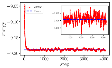
In Fig. 2 we show results for on a lattice with open boundary conditions. We first obtain a PEPS with cluster update, which gives . We then carry out a GFMC calculation with this PEPS as guiding wave function. As we can see from Fig. 2, the final converged energy () match the exact energy () within error bar, which is reasonable because there is no negative sign problem here. When there is no sign problem, the guiding PEPS wave function plays the role of important function whose quality only effect the sampling efficiency in GFMC.
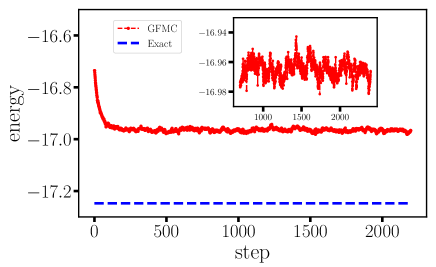
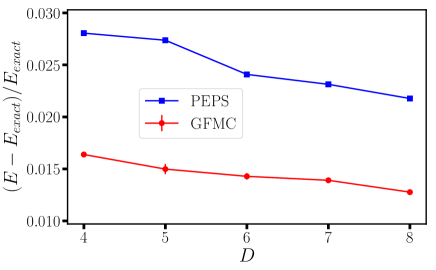
We then move to the more challenging case, where the negative sign problem emerges and we need to employ the fixed node approximation. In Fig. 3, we show the GFMC results for a system on lattice with OBC and , which represents the most difficulty region of the - Heisenberg model. A PEPS with from cluster update is taken as guiding wave function in GFMC. The variational energy for the PEPS is while the energy from GFMC is . This means the error to exact energy () is reduced nearly a half with GFMC in this case. In Fig. 4 we show the comparison of converged GFMC energy and the energy of the corresponding PEPS guiding wave function for a range of bond dimensions. We can see for all the values, the GFMC energies are lower than PEPS energy and the errors are reduced by about . We want to emphasize that is the most difficulty region for the - Heisenberg model. We anticipate that the improvement in other regions will be even larger (the result above is an example).
Usually in GFMC calculation, a variational Monte Carlo (VMC) calculation is performed at first to obtain the guiding wave function Runge (1992). TNS can be also viewed as variational wave functions. Nevertheless, the form of wave function needs to be specified in VMC, while TNS are more general and are systematically improvable with the increase of bond dimension Liao et al. (2017). Moreover, PEPS satisfy the area law Verstraete and Cirac (2004) by design.
Summary and perspectives – In conclusion, we proposed a new approach to study the ground state properties of quantum many-body systems in which TNS and GFMC are combined to take advantage of both of them. Benchmark results for - Heisenberg model on square lattice were provided to demonstrate the effectiveness of this method. One benefit to combine PEPS and GFMC is that only contraction of single-layer tensor network is needed which reduces the computational complexity substantially (from to ) and enable the reach of large bond dimension in PEPS, if the optimization process doesn’t involve contraction of double-layer tensor network. Nevertheless, after obtaining the optimized PEPS with full update, we can further improve the energy by taking it as guiding wave function, though the bottleneck is the optimization of PEPS itself in full update. The energy obtained in GFMC is guaranteed to be variational and lower than the PEPS guiding wave function. Our method can be improved in many aspects. With the stochastic reconfiguration technique Sorella and Capriotti (2000), the bias from guiding wave function can be reduced. We can generalize single PEPS guiding function to a linear combination of PEPS Huang et al. (2018) which can give lower variational energy. Generalization to fermionic systems is straightforward An and van Leeuwen (1991); van Bemmel et al. (1994). We only calculated ground state energy in this work, but excitation gaps can be calculated easily by enforcing symmetry, conservation of for example, in PEPS. Quantities other than energy can be calculated with the forward propagation technique Runge (1992) without increasing of computational complexity. Tensor Network States other than PEPS Shi et al. (2006); Vidal (2008); Xie et al. (2014) can also be adopted as guiding wave function. We believe that this new approach will provide us an accurate and efficient tool in the study of strongly correlated many-body systems in the future.
Acknowledgements.
This work is supported by a start-up fund from School of Physics and Astronomy in Shanghai Jiao Tong University. We thank Shiwei Zhang for previous discussions about the combination of TNS and QMC. We also acknowledge the support of computational resource by Shiwei Zhang at the Flatiron Institute.References
- Bednorz and Müller (1986) J. G. Bednorz and K. A. Müller, Zeitschrift für Physik B Condensed Matter 64, 189 (1986), ISSN 1431-584X, URL https://doi.org/10.1007/BF01303701.
- Tsui et al. (1982) D. C. Tsui, H. L. Stormer, and A. C. Gossard, Phys. Rev. Lett. 48, 1559 (1982), URL https://link.aps.org/doi/10.1103/PhysRevLett.48.1559.
- Laughlin (1983) R. B. Laughlin, Phys. Rev. Lett. 50, 1395 (1983), URL https://link.aps.org/doi/10.1103/PhysRevLett.50.1395.
- Zhou et al. (2017) Y. Zhou, K. Kanoda, and T.-K. Ng, Rev. Mod. Phys. 89, 025003 (2017), URL https://link.aps.org/doi/10.1103/RevModPhys.89.025003.
- Lieb and Wu (1968) E. H. Lieb and F. Y. Wu, Phys. Rev. Lett. 20, 1445 (1968), URL https://link.aps.org/doi/10.1103/PhysRevLett.20.1445.
- White (1992) S. R. White, Phys. Rev. Lett. 69, 2863 (1992), URL https://link.aps.org/doi/10.1103/PhysRevLett.69.2863.
- White (1993) S. R. White, Phys. Rev. B 48, 10345 (1993), URL https://link.aps.org/doi/10.1103/PhysRevB.48.10345.
- Schollwöck (2005) U. Schollwöck, Rev. Mod. Phys. 77, 259 (2005), URL https://link.aps.org/doi/10.1103/RevModPhys.77.259.
- Schollwöck (2011) U. Schollwöck, Annals of Physics 326, 96 (2011), ISSN 0003-4916, january 2011 Special Issue, URL http://www.sciencedirect.com/science/article/pii/S0003491610001752.
- Östlund and Rommer (1995) S. Östlund and S. Rommer, Phys. Rev. Lett. 75, 3537 (1995), URL https://link.aps.org/doi/10.1103/PhysRevLett.75.3537.
- Affleck et al. (1987) I. Affleck, T. Kennedy, E. H. Lieb, and H. Tasaki, Phys. Rev. Lett. 59, 799 (1987), URL https://link.aps.org/doi/10.1103/PhysRevLett.59.799.
- Baxter (1968) R. J. Baxter, Journal of Mathematical Physics 9, 650 (1968), eprint https://doi.org/10.1063/1.1664623, URL https://doi.org/10.1063/1.1664623.
- Eisert et al. (2010) J. Eisert, M. Cramer, and M. B. Plenio, Rev. Mod. Phys. 82, 277 (2010), URL https://link.aps.org/doi/10.1103/RevModPhys.82.277.
- Verstraete et al. (2008) F. Verstraete, V. Murg, and J. Cirac, Advances in Physics 57, 143 (2008), eprint https://doi.org/10.1080/14789940801912366, URL https://doi.org/10.1080/14789940801912366.
- Orús (2014) R. Orús, Annals of Physics 349, 117 (2014), ISSN 0003-4916, URL http://www.sciencedirect.com/science/article/pii/S0003491614001596.
- Chen et al. (2011) X. Chen, Z.-C. Gu, and X.-G. Wen, Phys. Rev. B 83, 035107 (2011), URL https://link.aps.org/doi/10.1103/PhysRevB.83.035107.
- Schuch et al. (2011) N. Schuch, D. Pérez-García, and I. Cirac, Phys. Rev. B 84, 165139 (2011), URL https://link.aps.org/doi/10.1103/PhysRevB.84.165139.
- Stoudenmire and White (2012) E. Stoudenmire and S. R. White, Annual Review of Condensed Matter Physics 3, 111 (2012), eprint https://doi.org/10.1146/annurev-conmatphys-020911-125018, URL https://doi.org/10.1146/annurev-conmatphys-020911-125018.
- Yan et al. (2011) S. Yan, D. A. Huse, and S. R. White, Science 332, 1173 (2011), ISSN 0036-8075, eprint https://science.sciencemag.org/content/332/6034/1173.full.pdf, URL https://science.sciencemag.org/content/332/6034/1173.
- LeBlanc et al. (2015) J. P. F. LeBlanc, A. E. Antipov, F. Becca, I. W. Bulik, G. K.-L. Chan, C.-M. Chung, Y. Deng, M. Ferrero, T. M. Henderson, C. A. Jiménez-Hoyos, et al. (Simons Collaboration on the Many-Electron Problem), Phys. Rev. X 5, 041041 (2015), URL https://link.aps.org/doi/10.1103/PhysRevX.5.041041.
- Zheng et al. (2017) B.-X. Zheng, C.-M. Chung, P. Corboz, G. Ehlers, M.-P. Qin, R. M. Noack, H. Shi, S. R. White, S. Zhang, and G. K.-L. Chan, Science 358, 1155 (2017), ISSN 0036-8075, eprint http://science.sciencemag.org/content/358/6367/1155.full.pdf, URL http://science.sciencemag.org/content/358/6367/1155.
- Qin et al. (2020) M. Qin, C.-M. Chung, H. Shi, E. Vitali, C. Hubig, U. Schollwöck, S. R. White, and S. Zhang (Simons Collaboration on the Many-Electron Problem), Phys. Rev. X 10, 031016 (2020), URL https://link.aps.org/doi/10.1103/PhysRevX.10.031016.
- Liang and Pang (1994) S. Liang and H. Pang, Phys. Rev. B 49, 9214 (1994), URL https://link.aps.org/doi/10.1103/PhysRevB.49.9214.
- Verstraete and Cirac (2004) F. Verstraete and J. I. Cirac, arXiv e-prints cond-mat/0407066 (2004), eprint cond-mat/0407066.
- Jiang et al. (2008) H. C. Jiang, Z. Y. Weng, and T. Xiang, Phys. Rev. Lett. 101, 090603 (2008), URL https://link.aps.org/doi/10.1103/PhysRevLett.101.090603.
- Jordan et al. (2008) J. Jordan, R. Orús, G. Vidal, F. Verstraete, and J. I. Cirac, Phys. Rev. Lett. 101, 250602 (2008), URL https://link.aps.org/doi/10.1103/PhysRevLett.101.250602.
- Corboz et al. (2011) P. Corboz, A. M. Läuchli, K. Penc, M. Troyer, and F. Mila, Phys. Rev. Lett. 107, 215301 (2011), URL https://link.aps.org/doi/10.1103/PhysRevLett.107.215301.
- Corboz et al. (2014) P. Corboz, T. M. Rice, and M. Troyer, Phys. Rev. Lett. 113, 046402 (2014), URL https://link.aps.org/doi/10.1103/PhysRevLett.113.046402.
- Liao et al. (2017) H. J. Liao, Z. Y. Xie, J. Chen, Z. Y. Liu, H. D. Xie, R. Z. Huang, B. Normand, and T. Xiang, Phys. Rev. Lett. 118, 137202 (2017), URL https://link.aps.org/doi/10.1103/PhysRevLett.118.137202.
- Gioev and Klich (2006) D. Gioev and I. Klich, Phys. Rev. Lett. 96, 100503 (2006), URL https://link.aps.org/doi/10.1103/PhysRevLett.96.100503.
- Orús and Vidal (2009) R. Orús and G. Vidal, Phys. Rev. B 80, 094403 (2009), URL https://link.aps.org/doi/10.1103/PhysRevB.80.094403.
- Phien et al. (2015) H. N. Phien, J. A. Bengua, H. D. Tuan, P. Corboz, and R. Orús, Phys. Rev. B 92, 035142 (2015), URL https://link.aps.org/doi/10.1103/PhysRevB.92.035142.
- Ran et al. (2007) Y. Ran, M. Hermele, P. A. Lee, and X.-G. Wen, Phys. Rev. Lett. 98, 117205 (2007), URL https://link.aps.org/doi/10.1103/PhysRevLett.98.117205.
- Depenbrock et al. (2012) S. Depenbrock, I. P. McCulloch, and U. Schollwöck, Phys. Rev. Lett. 109, 067201 (2012), URL https://link.aps.org/doi/10.1103/PhysRevLett.109.067201.
- Iqbal et al. (2013) Y. Iqbal, F. Becca, S. Sorella, and D. Poilblanc, Phys. Rev. B 87, 060405 (2013), URL https://link.aps.org/doi/10.1103/PhysRevB.87.060405.
- Mei et al. (2017) J.-W. Mei, J.-Y. Chen, H. He, and X.-G. Wen, Phys. Rev. B 95, 235107 (2017), URL https://link.aps.org/doi/10.1103/PhysRevB.95.235107.
- Blankenbecler et al. (1981) R. Blankenbecler, D. J. Scalapino, and R. L. Sugar, Phys. Rev. D 24, 2278 (1981), URL https://link.aps.org/doi/10.1103/PhysRevD.24.2278.
- Assaad and Evertz (2008) F. Assaad and H. Evertz, pp. 277–356 (2008), URL https://doi.org/10.1007/978-3-540-74686-7_10.
- Zhang (2004) S. Zhang, Quantum Monte Carlo Methods for Strongly Correlated Electron Systems (Springer New York, New York, NY, 2004), pp. 39–74, ISBN 978-0-387-21717-8, URL https://doi.org/10.1007/0-387-21717-7_2.
- Loh et al. (1990) E. Y. Loh, J. E. Gubernatis, R. T. Scalettar, S. R. White, D. J. Scalapino, and R. L. Sugar, Phys. Rev. B 41, 9301 (1990), URL https://link.aps.org/doi/10.1103/PhysRevB.41.9301.
- Troyer and Wiese (2005) M. Troyer and U.-J. Wiese, Phys. Rev. Lett. 94, 170201 (2005), URL https://link.aps.org/doi/10.1103/PhysRevLett.94.170201.
- Kalos (1962) M. H. Kalos, Phys. Rev. 128, 1791 (1962), URL https://link.aps.org/doi/10.1103/PhysRev.128.1791.
- Ceperley and Alder (1980) D. M. Ceperley and B. J. Alder, Phys. Rev. Lett. 45, 566 (1980), URL https://link.aps.org/doi/10.1103/PhysRevLett.45.566.
- Foulkes et al. (2001) W. M. C. Foulkes, L. Mitas, R. J. Needs, and G. Rajagopal, Rev. Mod. Phys. 73, 33 (2001), URL https://link.aps.org/doi/10.1103/RevModPhys.73.33.
- Zhang et al. (1997) S. Zhang, J. Carlson, and J. E. Gubernatis, Phys. Rev. B 55, 7464 (1997), URL https://link.aps.org/doi/10.1103/PhysRevB.55.7464.
- An and van Leeuwen (1991) G. An and J. M. J. van Leeuwen, Phys. Rev. B 44, 9410 (1991), URL https://link.aps.org/doi/10.1103/PhysRevB.44.9410.
- van Bemmel et al. (1994) H. J. M. van Bemmel, D. F. B. ten Haaf, W. van Saarloos, J. M. J. van Leeuwen, and G. An, Phys. Rev. Lett. 72, 2442 (1994), URL https://link.aps.org/doi/10.1103/PhysRevLett.72.2442.
- Capriotti et al. (1999) L. Capriotti, A. E. Trumper, and S. Sorella, Phys. Rev. Lett. 82, 3899 (1999), URL https://link.aps.org/doi/10.1103/PhysRevLett.82.3899.
- Chang and Zhang (2008) C.-C. Chang and S. Zhang, Phys. Rev. B 78, 165101 (2008), URL https://link.aps.org/doi/10.1103/PhysRevB.78.165101.
- Qin et al. (2016) M. Qin, H. Shi, and S. Zhang, Phys. Rev. B 94, 235119 (2016), URL https://link.aps.org/doi/10.1103/PhysRevB.94.235119.
- Chandra and Doucot (1988) P. Chandra and B. Doucot, Phys. Rev. B 38, 9335 (1988), URL https://link.aps.org/doi/10.1103/PhysRevB.38.9335.
- Dagotto and Moreo (1989) E. Dagotto and A. Moreo, Phys. Rev. Lett. 63, 2148 (1989), URL https://link.aps.org/doi/10.1103/PhysRevLett.63.2148.
- Capriotti and Sorella (2000) L. Capriotti and S. Sorella, Phys. Rev. Lett. 84, 3173 (2000), URL https://link.aps.org/doi/10.1103/PhysRevLett.84.3173.
- Sandvik (1997) A. W. Sandvik, Phys. Rev. B 56, 11678 (1997), URL https://link.aps.org/doi/10.1103/PhysRevB.56.11678.
- Jiang and Wiese (2011) F.-J. Jiang and U.-J. Wiese, Phys. Rev. B 83, 155120 (2011), URL https://link.aps.org/doi/10.1103/PhysRevB.83.155120.
- Sandvik and Evertz (2010) A. W. Sandvik and H. G. Evertz, Phys. Rev. B 82, 024407 (2010), URL https://link.aps.org/doi/10.1103/PhysRevB.82.024407.
- Mambrini et al. (2006) M. Mambrini, A. Läuchli, D. Poilblanc, and F. Mila, Phys. Rev. B 74, 144422 (2006), URL https://link.aps.org/doi/10.1103/PhysRevB.74.144422.
- Murg et al. (2009) V. Murg, F. Verstraete, and J. I. Cirac, Phys. Rev. B 79, 195119 (2009), URL https://link.aps.org/doi/10.1103/PhysRevB.79.195119.
- Yu and Kao (2012) J.-F. Yu and Y.-J. Kao, Phys. Rev. B 85, 094407 (2012), URL https://link.aps.org/doi/10.1103/PhysRevB.85.094407.
- Jiang et al. (2012) H.-C. Jiang, H. Yao, and L. Balents, Phys. Rev. B 86, 024424 (2012), URL https://link.aps.org/doi/10.1103/PhysRevB.86.024424.
- Mezzacapo (2012) F. Mezzacapo, Phys. Rev. B 86, 045115 (2012), URL https://link.aps.org/doi/10.1103/PhysRevB.86.045115.
- Hu et al. (2013) W.-J. Hu, F. Becca, A. Parola, and S. Sorella, Phys. Rev. B 88, 060402 (2013), URL https://link.aps.org/doi/10.1103/PhysRevB.88.060402.
- Gong et al. (2014) S.-S. Gong, W. Zhu, D. N. Sheng, O. I. Motrunich, and M. P. A. Fisher, Phys. Rev. Lett. 113, 027201 (2014), URL https://link.aps.org/doi/10.1103/PhysRevLett.113.027201.
- Morita et al. (2015) S. Morita, R. Kaneko, and M. Imada, Journal of the Physical Society of Japan 84, 024720 (2015), eprint https://doi.org/10.7566/JPSJ.84.024720, URL https://doi.org/10.7566/JPSJ.84.024720.
- Wang and Sandvik (2018) L. Wang and A. W. Sandvik, Phys. Rev. Lett. 121, 107202 (2018), URL https://link.aps.org/doi/10.1103/PhysRevLett.121.107202.
- Suzuki (1976) M. Suzuki, Progress of Theoretical Physics 56, 1454 (1976), ISSN 0033-068X, eprint https://academic.oup.com/ptp/article-pdf/56/5/1454/5264429/56-5-1454.pdf, URL https://doi.org/10.1143/PTP.56.1454.
- Pirvu et al. (2010) B. Pirvu, V. Murg, J. I. Cirac, and F. Verstraete, New Journal of Physics 12, 025012 (2010), URL https://doi.org/10.1088%2F1367-2630%2F12%2F2%2F025012.
- Evenbly (2018) G. Evenbly, Phys. Rev. B 98, 085155 (2018), URL https://link.aps.org/doi/10.1103/PhysRevB.98.085155.
- Wang and Verstraete (2011) L. Wang and F. Verstraete, arXiv e-prints arXiv:1110.4362 (2011), eprint 1110.4362.
- Xie et al. (2017) Z. Y. Xie, H. J. Liao, R. Z. Huang, H. D. Xie, J. Chen, Z. Y. Liu, and T. Xiang, Phys. Rev. B 96, 045128 (2017), URL https://link.aps.org/doi/10.1103/PhysRevB.96.045128.
- Corboz et al. (2010) P. Corboz, R. Orús, B. Bauer, and G. Vidal, Phys. Rev. B 81, 165104 (2010), URL https://link.aps.org/doi/10.1103/PhysRevB.81.165104.
- Carlson (1989) J. Carlson, Phys. Rev. B 40, 846 (1989), URL https://link.aps.org/doi/10.1103/PhysRevB.40.846.
- Trivedi and Ceperley (1989) N. Trivedi and D. M. Ceperley, Phys. Rev. B 40, 2737 (1989), URL https://link.aps.org/doi/10.1103/PhysRevB.40.2737.
- Trivedi and Ceperley (1990) N. Trivedi and D. M. Ceperley, Phys. Rev. B 41, 4552 (1990), URL https://link.aps.org/doi/10.1103/PhysRevB.41.4552.
- Runge (1992) K. J. Runge, Phys. Rev. B 45, 7229 (1992), URL https://link.aps.org/doi/10.1103/PhysRevB.45.7229.
- ten Haaf et al. (1995) D. F. B. ten Haaf, H. J. M. van Bemmel, J. M. J. van Leeuwen, W. van Saarloos, and D. M. Ceperley, Phys. Rev. B 51, 13039 (1995), URL https://link.aps.org/doi/10.1103/PhysRevB.51.13039.
- Calandra Buonaura and Sorella (1998) M. Calandra Buonaura and S. Sorella, Phys. Rev. B 57, 11446 (1998), URL https://link.aps.org/doi/10.1103/PhysRevB.57.11446.
- Schuch et al. (2007) N. Schuch, M. M. Wolf, F. Verstraete, and J. I. Cirac, Phys. Rev. Lett. 98, 140506 (2007), URL https://link.aps.org/doi/10.1103/PhysRevLett.98.140506.
- Nishino and Okunishi (1996) T. Nishino and K. Okunishi, Journal of the Physical Society of Japan 65, 891 (1996), eprint https://doi.org/10.1143/JPSJ.65.891, URL https://doi.org/10.1143/JPSJ.65.891.
- Levin and Nave (2007) M. Levin and C. P. Nave, Phys. Rev. Lett. 99, 120601 (2007), URL https://link.aps.org/doi/10.1103/PhysRevLett.99.120601.
- Gu and Wen (2009) Z.-C. Gu and X.-G. Wen, Phys. Rev. B 80, 155131 (2009), URL https://link.aps.org/doi/10.1103/PhysRevB.80.155131.
- Zhao et al. (2010) H. H. Zhao, Z. Y. Xie, Q. N. Chen, Z. C. Wei, J. W. Cai, and T. Xiang, Phys. Rev. B 81, 174411 (2010), URL https://link.aps.org/doi/10.1103/PhysRevB.81.174411.
- Lubasch et al. (2014) M. Lubasch, J. I. Cirac, and M.-C. Bañuls, Phys. Rev. B 90, 064425 (2014), URL https://link.aps.org/doi/10.1103/PhysRevB.90.064425.
- Xie et al. (2012) Z. Y. Xie, J. Chen, M. P. Qin, J. W. Zhu, L. P. Yang, and T. Xiang, Phys. Rev. B 86, 045139 (2012), URL https://link.aps.org/doi/10.1103/PhysRevB.86.045139.
- Evenbly and Vidal (2015) G. Evenbly and G. Vidal, Phys. Rev. Lett. 115, 180405 (2015), URL https://link.aps.org/doi/10.1103/PhysRevLett.115.180405.
- Yang et al. (2017) S. Yang, Z.-C. Gu, and X.-G. Wen, Phys. Rev. Lett. 118, 110504 (2017), URL https://link.aps.org/doi/10.1103/PhysRevLett.118.110504.
- Sandvik and Vidal (2007) A. W. Sandvik and G. Vidal, Phys. Rev. Lett. 99, 220602 (2007), URL https://link.aps.org/doi/10.1103/PhysRevLett.99.220602.
- Schuch et al. (2008) N. Schuch, M. M. Wolf, F. Verstraete, and J. I. Cirac, Phys. Rev. Lett. 100, 040501 (2008), URL https://link.aps.org/doi/10.1103/PhysRevLett.100.040501.
- Wang et al. (2011) L. Wang, I. Pižorn, and F. Verstraete, Phys. Rev. B 83, 134421 (2011), URL https://link.aps.org/doi/10.1103/PhysRevB.83.134421.
- Sikora et al. (2015) O. Sikora, H.-W. Chang, C.-P. Chou, F. Pollmann, and Y.-J. Kao, Phys. Rev. B 91, 165113 (2015), URL https://link.aps.org/doi/10.1103/PhysRevB.91.165113.
- Liu et al. (2017) W.-Y. Liu, S.-J. Dong, Y.-J. Han, G.-C. Guo, and L. He, Phys. Rev. B 95, 195154 (2017), URL https://link.aps.org/doi/10.1103/PhysRevB.95.195154.
- Zhao et al. (2017) H.-H. Zhao, K. Ido, S. Morita, and M. Imada, Phys. Rev. B 96, 085103 (2017), URL https://link.aps.org/doi/10.1103/PhysRevB.96.085103.
- du Croo de Jongh et al. (2000) M. S. L. du Croo de Jongh, J. M. J. van Leeuwen, and W. van Saarloos, Phys. Rev. B 62, 14844 (2000), URL https://link.aps.org/doi/10.1103/PhysRevB.62.14844.
- Wouters et al. (2014) S. Wouters, B. Verstichel, D. Van Neck, and G. K.-L. Chan, Phys. Rev. B 90, 045104 (2014), URL https://link.aps.org/doi/10.1103/PhysRevB.90.045104.
- Marshall and Peierls (1955) W. Marshall and R. E. Peierls, Proceedings of the Royal Society of London. Series A. Mathematical and Physical Sciences 232, 48 (1955), eprint https://royalsocietypublishing.org/doi/pdf/10.1098/rspa.1955.0200, URL https://royalsocietypublishing.org/doi/abs/10.1098/rspa.1955.0200.
- Sorella and Capriotti (2000) S. Sorella and L. Capriotti, Phys. Rev. B 61, 2599 (2000), URL https://link.aps.org/doi/10.1103/PhysRevB.61.2599.
- Huang et al. (2018) R.-Z. Huang, H.-J. Liao, Z.-Y. Liu, H.-D. Xie, Z.-Y. Xie, H.-H. Zhao, J. Chen, and T. Xiang, Chinese Physics B 27, 070501 (2018), URL https://doi.org/10.1088%2F1674-1056%2F27%2F7%2F070501.
- Shi et al. (2006) Y.-Y. Shi, L.-M. Duan, and G. Vidal, Phys. Rev. A 74, 022320 (2006), URL https://link.aps.org/doi/10.1103/PhysRevA.74.022320.
- Vidal (2008) G. Vidal, Phys. Rev. Lett. 101, 110501 (2008), URL https://link.aps.org/doi/10.1103/PhysRevLett.101.110501.
- Xie et al. (2014) Z. Y. Xie, J. Chen, J. F. Yu, X. Kong, B. Normand, and T. Xiang, Phys. Rev. X 4, 011025 (2014), URL https://link.aps.org/doi/10.1103/PhysRevX.4.011025.