Exploiting Diffuse Multipath in 5G SLAM

Abstract

5G millimeter wave (mmWave) signals can be used to jointly localize the receiver and map the propagation environment in vehicular networks, which is a typical simultaneous localization and mapping (SLAM) problem. Mapping the environment is challenging, due to measurements comprising both specular and diffuse multipath components, and diffuse multipath is usually considered as a perturbation. We here propose a novel method to utilize all available multipath signals from each landmark for mapping and incorporate this into a Poisson multi-Bernoulli mixture for the 5G SLAM problem. Simulation results demonstrate the efficacy of the proposed scheme.

I Introduction

5G mmWave communication is useful for localization and mapping, due to its geometric connection to the location of the user with respect to the base station (BS) and the propagation environment [1]. Signals from the BS can reach the user via multiple propagation paths. The channel estimation of each path provides accurate estimates of a time of arrival (TOA), angles of arrival (AOA), and angels of departure (AOD), which can be used to localize the user and map the environment [2].

Positioning and mapping using 5G signals is termed as 5G simultaneous localization and mapping (5G SLAM). The main tasks in 5G SLAM are to determine the user states (position, velocity, heading, clock bias) and to estimate the number of landmarks, their types and positions. In 5G SLAM, data association (DA) is an important problem, which is to assign the measurements to landmarks [3]. Landmarks in the environment can be smooth or rough surfaces [4]. Hence, in fact, each path (except the line-of-slight (LOS) path) is a cluster of paths, which may include a specular path and multiple diffuse paths.

The related works can be divided into two areas: works that exploit diffuse multipath for positioning or mapping and works in the area of 5G SLAM. In [5], diffuse multipath is seen as a perturbation, leading to false measurements. In [6], exploitation of the diffuse multipath in radar is proposed by means of including diffuse multipath statistics. In [7] surface roughness was considered in a radar applications, modeled as a number of sub-reflectors, in an environment with known wall geometry. A similar model with random sub-reflectors was evaluated in [8], where the estimated diffuse paths were used for positioning and mapping, but using a simple geometric approach. However, these methods do not solve the 5G SLAM problem over time or provide uncertainty information. The 5G SLAM problem has been addressed in a number of different approaches. In [9, 10], message passing-based estimators are introduced, which use the concept of nonparametric belief propagation, but the DA problem is not considered. A method based on random finite set and the probability hypothesis density (PHD) filters was proposed in [11]. Although this method considers the DA problem, there is no explicit enumeration of the different data associations. Moreover, in all these works, the landmarks are assumed to be perfect reflective surfaces or small scatter objects, with only one path for each landmark, so they ignore the information provided by diffuse multipath.

In this paper, we aim to harness the diffuse multipath components coming from rough surfaces in a 5G SLAM filter. The proposed scheme can estimate the vehicle location, orientation and clock bias as well as the locations and roughness of landmarks in the environment. The main contributions of this paper are summarized as follows: (i) We extend the filtering approach from [11] by utilizing a more powerful Poisson multi-Bernoulli mixture (PMBM) filter, and by considering a likelihood with multiple channel parameter estimates per surface; (ii) We derive a novel likelihood function for channel estimation from [8] of the cluster of paths from rough surfaces, for different types of surfaces with different roughness.

II Model

We describe the model of the vehicle (user), environment, received waveform, and channel parameter estimates.

II-A Vehicle Model

We consider a single vehicle in the environment, with a dynamic state $\boldsymbol{s}_{k}$ at time $k$, which comprises 3D position $\boldsymbol{x}_{\mathrm{UE},k}=[x_{k},y_{k},z_{k}]^{\mathsf{T}}$, heading $\alpha_{k}$, translation speed $\zeta_{k}$, turn rate $\rho_{k}$ and clock bias $B_{k}$. The transition density $f(\boldsymbol{s}_{k}|\boldsymbol{s}_{k-1})$ is derived from the following state model of $\boldsymbol{s}_{k}$

$$\boldsymbol{s}_{k}=\boldsymbol{v}(\boldsymbol{s}_{k-1})+\boldsymbol{q}_{k},$$ (1)

where $\boldsymbol{v}(\cdot)$ is a known transition function; $\boldsymbol{q}_{k}$ is the process noise, modeled as a zero-mean Gaussian with known covariance $\boldsymbol{Q}_{k}$.

II-B Environment Model

There is a fixed BS, with a known location $\boldsymbol{x}_{\mathrm{BS}}\in\mathbb{R}^{3}$ in the environment. The unknown environment is modeled as surfaces with different roughness (see Fig. 1). The roughness determines the amount of diffuse multipath components. We model each surface with three related parameters: the scattering power $S\geq 0$ (which determines the fraction of power that is scattered), the reflection power $R\geq 0$ (which determines the fraction of power that is reflected, with $R+S\leq 1$, as some of the power can be absorbed) and the smoothness parameter $\alpha_{\mathrm{R}}\geq 0$ (which determines the spread of the diffuse multipath) [8]. The state of a surface $\boldsymbol{x}$ can therefore be described by these three parameters and the fixed virtual anchor (VA), located at $\boldsymbol{x}_{\mathrm{VA}}\in\mathbb{R}^{3}$, which is the reflection of the BS with respect to the surface.

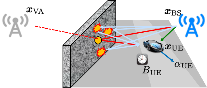
Figure 1: Scenario with the environment of a BS, a surface, and a vehicle. The existence of the specular path (shown as the red line) or the diffusion path (shown as the azure line) is depend on the type of the surface.

II-C Signal Model

The received signal sent from the BS to the vehicle at time $k$ can be modeled as[12]

$$\boldsymbol{y}_{k}(t)= (\boldsymbol{W}_{k})^{\mathsf{H}}\sum_{i=0}^{I_{k}-1}\sum_{l=0}^{L_{k}^{i}-1}g_{k}^{i,l}$$ (2)

$$\boldsymbol{a}_{\text{R}}(\boldsymbol{\theta}_{k}^{i,l})\boldsymbol{a}_{\text{T}}^{\mathsf{H}}(\boldsymbol{\phi}_{k}^{i,l})\boldsymbol{p}_{k}(t-\tau_{k}^{i,l})+\boldsymbol{r}_{k}(t),$$

where $\boldsymbol{p}_{k}(t)$ is the transmitted signal vector; $\boldsymbol{y}_{k}(t)$ is the received signal vector; $\boldsymbol{r}_{k}(t)$ is the noise vector; $\boldsymbol{W}_{k}$ is a combining matrix; $I_{k}$ is the number of landmarks in the environment. The landmark with index $i=0$ is the BS; $L_{k}^{i}$ is the number of paths from each landmark. Each path $l$ can be described by a complex gain $g_{k}^{i,l}$, a TOA $\tau_{k}^{i,l}$, an AOA pair $\boldsymbol{\theta}_{k}^{i,l}$ in azimuth and elevation, and an AOD pair $\boldsymbol{\phi}_{k}^{i,l}$ in azimuth and elevation; $\boldsymbol{a}_{\text{R}}(\cdot)$ and $\boldsymbol{a}_{\text{T}}(\cdot)$ are the steering vectors of the receiver and transmitter antenna arrays. The TOA, AOA and AOD depend on the locations of the transmitter, the receiver, and the incident points of NLOS paths in the environment. The number of paths per surface and their spread in angle and delay as well as the channel gains depend on the roughness of that surface. Conceptually, these paths can be interpreted as coming from random points on the surface, with a spatial distribution that depends on the roughness. Among the paths, there may be a deterministic specular component, while all remaining paths are diffuse components and thus random [8].

II-D Measurement Model

The vehicle executes a channel estimation routine, which aims to extract the angles and delays from the received signal. As the receiver has finite resolution, not all paths can be resolved. Hence, for each surface, the number of estimated paths will be much smaller than $L_{k}^{i}$. We assume the channel estimator provides a set of channel parameter estimates $\mathcal{Z}_{k}$ at time $k$, which is already grouped into clusters based on different sources, $\{\mathcal{Z}_{k}^{0},\mathcal{Z}_{k}^{1},\dots,\mathcal{Z}_{k}^{\hat{I}_{k}-1}\}$, where $\hat{I}_{k}$ is the number of estimated clusters. Each element $\boldsymbol{z}_{k}^{i,l}\in\mathcal{Z}_{k}^{i}$ is either clutter, which is caused by noise peaks, with clutter intensity $c(\boldsymbol{z})$ or follows

$$\boldsymbol{z}_{k}^{i,l}=\boldsymbol{h}(\boldsymbol{x}_{k}^{i,l},\boldsymbol{s}_{k})+\boldsymbol{w}_{k}^{i,l},$$ (3)

where $\boldsymbol{w}_{k}^{i,l}$ is measurement noise, and $\boldsymbol{x}_{k}^{i,l}$ is a point on the surface (either the incidence point of the deterministic specular components or a random point on the surface for a diffuse component), with $\boldsymbol{h}(\boldsymbol{x}_{k}^{i,l},\boldsymbol{s}_{k})=[\tau_{k}^{i,l},(\boldsymbol{\theta}_{k}^{i,l})^{\mathsf{T}},(\boldsymbol{\phi}_{k}^{i,l})^{\mathsf{T}}]^{\mathsf{T}}$, where the angles and delays depend on the underlying geometry.

Our goal is to estimate vehicle states and landmark states. It is challenging due to the random nature of the diffuse multipath, which in turn makes it challenging to describe the likelihood function $\ell(\mathcal{Z}_{k}^{i}|\boldsymbol{x}^{i},\boldsymbol{s}_{k})$, needed for the SLAM method. We will propose a landmark state $\boldsymbol{x}^{i}$ and likelihood function in Section IV.

III PMBM SLAM Filter

III-A Basics of PMBM Density

The PMBM filter relies on a PMBM density representation of the landmarks, conditioned on the vehicle state. A PMBM RFSs $\mathcal{X}$ can be viewed as the union of two disjoint RFS, the set of undetected objects $\mathcal{X}_{\mathrm{U}}$ and the set of detected objects $\mathcal{X}_{\mathrm{D}}$[13]. The undetected objects are the objects that have never been detected before; the detected objects are the objects that have been detected at least once before. We model $\mathcal{X}_{\mathrm{U}}$ as a Poisson point process (PPP), $\mathcal{X}_{\mathrm{D}}$ as a multi-Bernoulli mixture (MBM). The details of the densities of PPP and MBM can be found in [14, 13, 15]. Then, $f(\mathcal{X})$ can be defined by [16]

$$f(\mathcal{X})=\sum_{\mathcal{X}_{\mathrm{U}}\biguplus\mathcal{X}_{\mathrm{D}}=\mathcal{X}}f_{\mathrm{P}}(\mathcal{X}_{\mathrm{U}})f_{\mathrm{MBM}}(\mathcal{X}_{\mathrm{D}}),$$ (4)

where $\biguplus$ stands for the union of mutually disjoint sets; $f_{\mathrm{P}}(\cdot)$ is a PPP density; $f_{\mathrm{MBM}}(\cdot)$ is an MBM density. The PPP density is

$$f_{\mathrm{P}}(\mathcal{X}_{\mathrm{U}})=e^{-\int\lambda(\boldsymbol{x})d\boldsymbol{x}}\prod_{j=1}^{n}\lambda(\boldsymbol{x}^{j}),$$ (5)

where $\lambda(\cdot)$ is the intensity function; $n$ is the cardinality of $\mathcal{X}_{\mathrm{U}}$. The MBM density follows

$$f_{\mathrm{MBM}}(\mathcal{X}_{\mathrm{D}})\propto\sum_{h}\sum_{\mathcal{X}^{1}\biguplus\dots\biguplus\mathcal{X}^{n}=\mathcal{X}_{\mathrm{D}}}\prod_{j=1}^{n}l^{h,j}f^{h,j}_{\mathrm{B}}(\mathcal{X}^{j}),$$ (6)

where $h$ is the index for hypotheses [14]; $n$ is the number of potentially detected objects; $f_{\mathrm{B}}^{h,j}(\cdot)$ is the Bernoulli density of the object $j$ under the global hypothesis $h$, and $l^{h,j}$ is its weight. Each Bernoulli follows

$$f^{h,j}_{\mathrm{B}}(\mathcal{X}^{j})=\begin{cases}1-r^{h,j}\quad&\mathcal{X}^{j}=\emptyset\\ r^{h,j}f^{h,j}(\boldsymbol{x})\quad&\mathcal{X}^{j}=\{\boldsymbol{x}\}\end{cases}$$ (7)

and $f^{h,j}_{\mathrm{B}}(\mathcal{X}^{j})=0$ otherwise. Here, $r^{h,j}$ is the existence probability and $f^{h,j}(\cdot)$ is the state density. Then, (5) can be parameterized by $\lambda(\boldsymbol{x})$, and (6) can be parameterized by $\{l^{h,j},\{r^{h,j},f^{h,j}(\boldsymbol{x})\}_{j\in\mathbb{I}^{h}}\}_{h\in\mathbb{I}}$, where $\mathbb{I}$ is the index set.

The PMBM filter follows the prediction and update steps of the Bayesian filtering recursion with RFSs, using the Chapman-Komogorov applied to sets [17]. This then translates into prediction and update steps of the PMBM parameters $\lambda(\boldsymbol{x})$ and $\{l^{h,j},\{r^{h,j},f^{h,j}(\boldsymbol{x})\}_{j\in\mathbb{I}^{h}}\}_{h\in\mathbb{I}}$.

III-B Implementation of PMBM SLAM Filter

We follow the Rao-Blackwellized approach, where we use a group of particles to represent the vehicle state, and use PMBM densities conditioned on each particles to represent the map. Given a landmark state $\boldsymbol{x}$ with the measurement cluster $\mathcal{Z}_{k}^{i}$ at time $k$, we assume we are given a likelihood $\ell(\mathcal{Z}_{k}^{i}|\boldsymbol{x},\boldsymbol{s}_{k})$. This likelihood will be derived in the next section. We assume at the end of time $k$, there are $N$ particles $\boldsymbol{s}_{0:k}^{n}$ with non-negative weights $\omega_{k|k}^{n}$, $\sum_{n}\omega_{k|k}^{n}=1$, where for each particle $n$ we have a PMBM density with PPP parameter $\lambda^{n}_{k|k}(\boldsymbol{x})$ and MBM parameters $\{l_{k|k}^{n,h,j},\{r_{k|k}^{n,h,j},f_{k|k}^{n,h,j}(\boldsymbol{x})\}_{j\in\mathbb{I}_{k}^{n,h}}\}_{h\in\mathbb{I}_{k}^{n}}$. For simplicity, we drop the particle index $n$ in map prediction and map update.

III-B1 Vehicle Prediction

The state of ${n}^{\mathrm{th}}$ particle $\boldsymbol{s}_{k-1|k-1}^{n}$ is predicted using (1), yielding $\boldsymbol{s}_{k|k-1}^{n}=\boldsymbol{v}(\boldsymbol{s}_{k-1|k-1}^{n})+\boldsymbol{q}^{n}_{k}$, where $\boldsymbol{q}^{n}_{k}\sim\mathcal{N}(\boldsymbol{0},\boldsymbol{Q}_{k})$ and $\omega_{k|k-1}^{n}=\omega_{k-1|k-1}^{n}$.

III-B2 Map Prediction

The positions of landmarks are fixed, so we do not need to predict the state. The prediction of PPP intensity is $\lambda_{k|k-1}(\boldsymbol{x})=p_{\text{S}}\lambda_{k-1|k-1}(\boldsymbol{x})+\lambda_{\mathrm{B},k}(\boldsymbol{x})$ [18], where $p_{\mathrm{S}}$ is the survival probability (assumed as a constant for simplicity), $\lambda_{\mathrm{B},k}(\boldsymbol{x})$ is the intensity of the birth model. For the MBM components, the prediction step is $l_{k|k-1}^{h,j}=l_{k-1|k-1}^{h,j}$ for the weight, and $r_{k|k-1}^{h,j}=p_{\mathrm{S}}r_{k-1|k-1}^{h,j}$, $f_{k|k-1}^{h,j}(\boldsymbol{x})=f_{k-1|k-1}^{h,j}(\boldsymbol{x})$ for the density [18].

III-B3 Map Update

The update step uses the measurements to correct the landmarks’ positions and types. The update step consists of four cases [18]:

• Undetected objects that remain undetected by $\lambda_{k|k}(\boldsymbol{x})=(1-p_{\mathrm{D}})\lambda_{k|k-1}(\boldsymbol{x})$, where $p_{\mathrm{D}}$ is the detection probability (also assumed as a constant).

• Undetected objects that are detected for the first time using grouped measurement $\mathcal{Z}_{k}^{i}$:

  $$r_{\mathrm{U},k|k}^{i}=\rho_{\mathrm{U},k|k-1}^{i}(\mathcal{Z}_{k}^{i})/(c(\mathcal{Z}_{k}^{i})+\rho_{\mathrm{U},k|k-1}^{i}(\mathcal{Z}_{k}^{i}))$$

  $$f_{\mathrm{U},k|k}^{i}(\boldsymbol{x})=p_{\mathrm{D}}\ell(\mathcal{Z}_{k}^{i}|\boldsymbol{x},\boldsymbol{s}_{k|k-1})\lambda_{k|k-1}(\boldsymbol{x})/\rho_{\mathrm{U},k|k-1}^{i}(\mathcal{Z}_{k}^{i})$$

  $$l_{\mathrm{U},k|k}^{i}=c(\mathcal{Z}_{k}^{i})+\rho_{\mathrm{U},k|k-1}^{i}(\mathcal{Z}_{k}^{i})$$

  $$\rho_{\mathrm{U},k|k-1}^{i}(\mathcal{Z}_{k}^{i})=\int p_{\mathrm{D}}\ell(\mathcal{Z}_{k}^{i}|\boldsymbol{x},\boldsymbol{s}_{k|k-1})\lambda_{k|k-1}(\boldsymbol{x})\text{d}\boldsymbol{x},$$

  where $c(\mathcal{Z}_{k}^{i})=\delta(|\mathcal{Z}_{k}^{i}|=1)c(\boldsymbol{z}^{i,0}_{k})$. Note that $h$ and $j$ do not appear, since the object was undetected before (indicated by the notation ${\mathrm{U}}$).

• Previously detected objects that are misdetected:

  $$r_{k|k}^{h,j,0}=(1-p_{\mathrm{D}})r_{k|k-1}^{h,j}/(1-p_{\mathrm{D}}r_{k|k-1}^{h,j})$$

  $$f_{k|k}^{h,j,0}(\boldsymbol{x})=f_{k|k-1}^{h,j}(\boldsymbol{x})$$

  $$l_{k|k}^{h,j,0}=l_{k|k-1}^{h,j}(1-r_{k|k-1}^{h,j}p_{\mathrm{D}}).$$

• Previously detected objects that are detected again using set $\mathcal{Z}_{k}^{i}$:

  $$r_{k|k}^{h,j,i}=1$$

  $$f_{k|k}^{h,j,i}(\boldsymbol{x})=p_{\mathrm{D}}\ell(\mathcal{Z}_{k}^{i}|\boldsymbol{x},\boldsymbol{s}_{k|k-1})f_{k|k-1}^{h,j}(\boldsymbol{x})/\rho_{k|k-1}^{h,j,i}(\mathcal{Z}_{k}^{i})$$

  $$l_{k|k}^{h,j,i}=l_{k|k-1}^{h,j}r_{k|k-1}^{h,j}\rho_{k|k-1}^{h,j,i}(\mathcal{Z}_{k}^{i})$$

  $$\rho_{k|k-1}^{h,j,i}(\mathcal{Z}_{k}^{i})=\int p_{\mathrm{D}}\ell(\mathcal{Z}_{k}^{i}|\boldsymbol{x},\boldsymbol{s}_{k|k-1})f_{k|k-1}^{h,j}(\boldsymbol{x})\text{d}\boldsymbol{x}.$$

To avoid the exponential complexity associated with introducing new landmarks for each measurement, hypotheses can be removed, e.g., based on Murty’s algorithm [19], where weights $l_{\mathrm{U},k|k}^{i}$, $l_{k|k}^{h,j,0}$ and $l_{k|k}^{h,j,i}$ calculated in III-B3 construct a cost matrix [13].

III-B4 Vehicle Update

Each particle weight can be update by $\omega_{k|k}^{n}\propto\omega_{k|k-1}^{n}\sum_{h}l_{k|k}^{n,h}$, where $l_{k|k}^{n,h}$ is the weight of updated global hypothesis $h$ for particle $n$, given by the Murty’s algorithm. The estimate vehicle state is given by $\hat{\boldsymbol{s}}_{k|k}=\sum_{n}\omega_{k|k}^{n}\boldsymbol{s}_{k|k}^{n}$. Finally, the resampling of particles can be applied.

IV Likelihood function derivation

For brevity, we will omit the time index $k$ and the particle index $n$.

IV-A Assumptions

In order to derive the likelihood function $\ell(\mathcal{Z}^{i}|\boldsymbol{x},\boldsymbol{s})$ needed in the PMBM SLAM filter, we make several additional assumptions:

• Channel estimation method: We consider the channel estimator in [8], which uses a tensor ESPRIT-based method to estimate 5G channel parameters in the presence of combined specular and diffuse multipath from the surface. With this specific channel estimator, we can generate simulated data to determine the likelihood function.

• State representation: In order to have a compact state representation, we consider 3 different types of surfaces: smooth surface (SM, with $S=0$, $R=0.8$, $\alpha_{\mathrm{R}}=100$), medium rough surface (MR, with $S=0.4,R=0.6,\alpha_{\mathrm{R}}=4$) and very rough surface (VR, with $S=0.8,R=0,\alpha_{\mathrm{R}}=0$). This allows us to set the landmark state to $\boldsymbol{x}=[\boldsymbol{x}^{\textsf{T}}_{\text{LM}},m]^{\textsf{T}}$, where $m\in\{\text{BS},\text{SM},\text{MR},\text{VR}\}$ and $\boldsymbol{x}_{\text{LM}}=\boldsymbol{x}_{\text{BS}}$ for $m=\text{BS}$, while $\boldsymbol{x}_{\text{LM}}=\boldsymbol{x}_{\text{VA}}$, for $m\neq\text{BS}$. Hence, we can write $\ell(\mathcal{Z}^{i}|\boldsymbol{x}_{\text{LM}},\boldsymbol{s},m)$.

• Measurement independence: We assume that the measurements within the set $\mathcal{Z}^{i}$ are independent, though not necessarily identically distributed, since scatter points are generated independently. For simplicity, we also assume that the number of measurements $|\mathcal{Z}^{i}|$ only depends on $m$.

IV-B Likelihood Function

With these assumptions, the likelihood function is

$$\ell(\mathcal{Z}^{i}|\boldsymbol{x}_{\mathrm{LM}},\boldsymbol{s},m)$$

$$=p(|\mathcal{Z}^{i}||m)\prod^{|\mathcal{Z}^{i}|-1}_{l=0}p(\boldsymbol{z}^{i,l}|\boldsymbol{x}_{\text{LM}},\boldsymbol{s},m).$$ (8)

We would like to express this likelihood in a form compatible with (3), i.e., as a function of an incidence point on the surface for $m\neq\text{BS}$ or as a function of the BS location for $m=\text{BS}$.

IV-B1 Case $m=\text{BS}$

In this case $|\mathcal{Z}^{i}|=1$ and

$$\ell(\mathcal{Z}^{i}=\{\boldsymbol{z}^{i,0}\}|\boldsymbol{x}_{\mathrm{LM}},\boldsymbol{s},m=\text{BS})=p(\boldsymbol{z}^{i,0}|\boldsymbol{x}_{\text{BS}},\boldsymbol{s}),$$ (9)

which is in the desired form.

IV-B2 Case $m\neq\text{BS}$

The incidence point on the surface of a specular component can be derived from Snell’s law of reflection, and is given by the intersection of the line between the VA location $\boldsymbol{x}_{\mathrm{LM}}$ and the UE location $\boldsymbol{x}_{\mathrm{UE}}$ with the surface:

$$\boldsymbol{x}_{0}=\boldsymbol{x}_{\mathrm{LM}}+\frac{(\boldsymbol{x}_{e}-\boldsymbol{x}_{\mathrm{LM}})^{\textsf{T}}\boldsymbol{e}}{(\boldsymbol{x}_{\mathrm{UE}}-\boldsymbol{x}_{\mathrm{LM}})^{\textsf{T}}\boldsymbol{e}}(\boldsymbol{x}_{\mathrm{UE}}-\boldsymbol{x}_{\mathrm{LM}}),$$ (10)

where $\boldsymbol{x}_{e}=({\boldsymbol{x}_{\mathrm{BS}}+\boldsymbol{x}_{\mathrm{LM}}})/{2}$ is a point on the surface, and $\boldsymbol{e}=({\boldsymbol{x}_{\mathrm{BS}}-\boldsymbol{x}_{\mathrm{LM}}})/{\left\|\boldsymbol{x}_{\mathrm{BS}}-\boldsymbol{x}_{\mathrm{LM}}\right\|}$ is a normal to the surface. We now separate $\mathcal{Z}^{i}$ into two parts, the path with the shortest delay $\boldsymbol{z}^{i,0}$, and the remaining paths $\{\boldsymbol{z}^{i,1},\boldsymbol{z}^{i,2},\dots,\boldsymbol{z}^{i,|\mathcal{Z}^{i}|-1}\}$. Since $\boldsymbol{z}^{i,0}$ is the path closest to the specular component we associate it with the deterministic incidence point $\boldsymbol{x}_{0}$. The remaining paths are associated with random incidence points on the surface. Therefore, we write for $\boldsymbol{z}^{i,0}$ that $p(\boldsymbol{z}^{i,0}|\boldsymbol{x}_{\text{LM}},\boldsymbol{s},m)=p(\boldsymbol{z}^{i,0}|\boldsymbol{x}_{0},\boldsymbol{s},m)$, which is in the desired form.

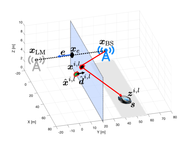
Figure 2: The principle of how to calculate $\hat{d}^{i,l}$ using $\boldsymbol{z}^{i,l}$, $\boldsymbol{x}_{\mathrm{LM}}$ and $\boldsymbol{x}_{\mathrm{BS}}$, when $m\neq\text{BS}$. We use one path $l$ as an example.

For diffuse paths $l>0$, the incidence point on the surface is unknown. We proceed as follows. From $\boldsymbol{z}^{i,l}$, we compute a position $\hat{\boldsymbol{x}}^{i,l}\in\mathbb{R}^{3}$, using the method in [20]. This position is a function of $\boldsymbol{s}$ and $\boldsymbol{z}^{i,l}$. In the absence of uncertainty, which is caused by the measurement noise and the interpath interference, $\hat{\boldsymbol{x}}^{i,l}$ would lie on the surface. As we don’t know the random incidence points that gave rise to $\boldsymbol{z}^{i,l}$, our best guess is the projection of $\hat{\boldsymbol{x}}^{i,l}$ onto the surface, i.e., $\tilde{\boldsymbol{x}}^{i,l}=\hat{\boldsymbol{x}}^{i,l}+(\boldsymbol{x}_{e}-\hat{\boldsymbol{x}}^{i,l})^{\textsf{T}}\boldsymbol{e}~{}\boldsymbol{e}$. We then have $p(\boldsymbol{z}^{i,l}|\boldsymbol{x}_{\text{LM}},\boldsymbol{s},m)=p(\boldsymbol{z}^{i,l}|\tilde{\boldsymbol{x}}^{i,l}),~{}l>0$, where $\tilde{\boldsymbol{x}}^{i,l}$ is the assumed incidence point that gave rise to measurement $\boldsymbol{z}^{i,l}$. Since the only non-zero error component in this likelihood function is the one orthogonal to the surface, we use it directly as a compressed measurement

$$\hat{d}^{i,l}(\boldsymbol{z}^{i,l})=\boldsymbol{e}^{\mathsf{T}}(\hat{\boldsymbol{x}}^{i,l}-\boldsymbol{x}_{e}).$$ (11)

Fig. 2 shows the principle of calculating $\hat{d}^{i,l}(\boldsymbol{z}^{i,l})$. Therefore, the overall likelihood function is

$$\ell({\mathcal{Z}^{i}}|\boldsymbol{x}_{\mathrm{LM}},\boldsymbol{s},m)=$$ (12)

$$p(|\mathcal{Z}^{i}||m)p(\boldsymbol{z}^{i,0}|\boldsymbol{x}_{\mathrm{LM}},\boldsymbol{s},m)\prod^{|\mathcal{Z}^{i}|-1}_{l=1}p(\hat{d}^{i,l}(\boldsymbol{z}^{i,l})|\boldsymbol{x}_{\mathrm{LM}},\boldsymbol{s},m),$$

where all distributions can be obtained from the simulation of a channel estimator or provided directly in closed-form by a channel estimator.

V Results

V-A Scenario

We consider a scenario with a single BS and a vehicle. During $k=40$ time steps, the BS sends $10\times 64$ OFDM symbols to the vehicle with 200 subcarriers using the transmit power of 5.05 W at each time step; the subcarrier spacing is 0.5 MHz; the noise power spectral density is $4.0049\times 10^{-9}$ mW/Hz; the carrier frequency is 28 GHz. The transmitter and the receiver are both equipped with a uniform rectangular array (URA) with $8\times 8$ antennas.

As shown in Fig. 3, there are a SM, two MRs, and a VR in the environment, which can reflect or/and diffuse signals to the vehicle. The vehicle has a known constant turn rate movement around the BS. The movement has the same transition function as in [11, eq. 38]. The initial vehicle state is $[70.7285,0,0,\pi/2,22.22,\pi/10,300]^{\mathrm{T}}$; the process noise, the initial prior, the survival probability, the detection probability, the birth rate, the clutter intensity, and pruning thresholds are the same as in [11]. We adopt the generalized optimal subpattern assignment (GOSPA) distance [21] as the metric for evaluating the mapping result, and the parameter settings for calculating GOSPA distance are the same as in [11].

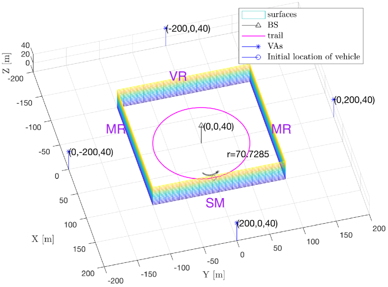
Figure 3: Scenario with the environment of a BS and 4 surfaces. A vehicle moves counterclockwise along the trail.

TABLE I: Likelihood function for 5G SLAM for different surface types

Type ${m}$	$p(|\mathcal{Z}^{i}||m)$	$p(\boldsymbol{z}^{i,0}|\boldsymbol{x}_{\text{LM}},\boldsymbol{s},m)$	$p(\hat{d}^{i,l}|\boldsymbol{x}_{\mathrm{LM}},\boldsymbol{s},m)$
BS	$|\mathcal{Z}^{i}|\sim\delta(1)$	$\mathcal{N}(\boldsymbol{z}^{i,0};\boldsymbol{h}_{\mathrm{BS}},\mathrm{diag}([0.003,0.0001\times\boldsymbol{1}_{4}]^{2}))$	N/A
SM	$|\mathcal{Z}^{i}|\sim\delta(1)$	$\mathcal{N}(\boldsymbol{z}^{i,0};\boldsymbol{h}_{\mathrm{VA}},\mathrm{diag}([0.01,0.002\times\boldsymbol{1}_{4}]^{2}))$	N/A
MR	$(|\mathcal{Z}^{i}|-2)\sim\text{Geo}(0.55)$	$\mathcal{N}(\boldsymbol{z}^{i,0};\boldsymbol{h}_{\mathrm{VA}}+[0.07,\boldsymbol{0}_{1\times 4}]^{\mathrm{T}},\mathrm{diag}([0.1,0.008\times\boldsymbol{1}_{4}]^{2}))$	$\mathcal{N}(\hat{d}^{i,l};0.435,0.3^{2})$
VR	$(|\mathcal{Z}^{i}|-4)\sim\text{Geo}(0.27)$	$\mathcal{N}(\boldsymbol{z}^{i,0};\boldsymbol{h}_{\mathrm{VA}}+[0.8,\boldsymbol{0}_{1\times 4}]^{\mathrm{T}},\mathrm{diag}([0.5,0.05\times\boldsymbol{1}_{4}]^{2}))$	$\mathcal{N}(\hat{d}^{i,l};0.435,0.3^{2})$
$\boldsymbol{h}_{\mathrm{BS}}$, $\boldsymbol{h}_{\mathrm{VA}}$ are the geometric relations $\boldsymbol{h}(\boldsymbol{x}_{\mathrm{BS}},\boldsymbol{s})$ and $\boldsymbol{h}(\boldsymbol{x}_{\mathrm{VA}},\boldsymbol{s})$, which can be found in [11, Appendix A].

V-B Experimental Likelihood Function

All three components in $\eqref{likelihoodfunction_final}$ for different sources are acquired by investigating the statistics of the simulation results of the ESPRIT estimator [8] using the environment settings in this paper.

To gain intuition, we will focus on the case $m=\text{VR}$ and analyze $p(|\mathcal{Z}^{i}||\text{VR})$, $p(\tau^{i,0}|\boldsymbol{x}_{\text{LM}},\boldsymbol{s},\text{VR})$ and $p(\hat{d}^{i,l}|\boldsymbol{x}_{\text{LM}},\boldsymbol{s},\text{VR})$, based on data gathered from the ESPRIT estimator in various UE locations. Fig. 4 shows the histogram of the number of paths, as well as a geometric fit. We observe that at least 4 paths are always present, while up to 13 paths can be resolved for very rough surfaces.

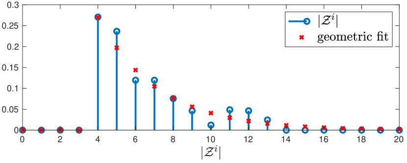
Figure 4: Geometric fit for $p(|\mathcal{Z}^{i}||\mathrm{VR})$.

Fig. 5 shows the histogram of the delay of the first estimated path $\tau^{i,0}$ (subtracted with the delay of the specular path) as well as a Gaussian approximation. We observe that there is interpath interference, which leads to a shift of delay of 0.8 m.

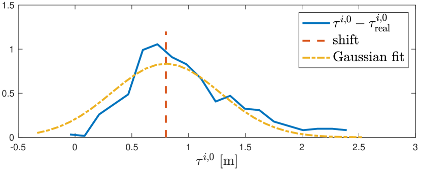
Figure 5: Histogram and Gaussian fit for $p(\tau^{i,0}|\boldsymbol{x}_{\text{LM}},\boldsymbol{s},\mathrm{VR})$.

Finally, Fig. 6 shows the histogram and Gaussian fit of the distances $\hat{d}^{i,l},~{}l>0$. We observe that the estimated scatter points are more likely to be behind the surface, due to the delay shift.

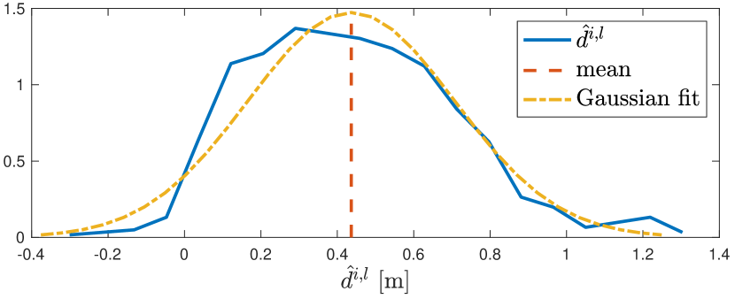
Figure 6: Histogram and Gaussian fit for $p(\hat{d}^{i,l}|\boldsymbol{x}_{\text{LM}},\boldsymbol{s},\mathrm{VR})$.

A complete overview of the likelihood function for all surface types as well as LOS is provided in Table I. We make the following observations: there is one path present, and the measurement of the path follows Gaussian distribution for both cases $m=\text{BS}$ and $m=\text{SM}$; there are 2 to 6 paths present, and the measurement of the specular path and the distance follow Gaussian distributions for the case $m=\text{MR}$.

V-C SLAM Results and Discussions

Firstly, we study the performance of the proposed 5G SLAM scheme in mapping. We use the real vehicle states and compare the mapping results of two algorithms: (1) SLAM filter using all paths in every signal cluster based on the proposed likelihood function; (2) SLAM filter using the single (specular) path in every cluster. From Fig. 7, we could find both algorithms perform similarly in mapping the SM. This is because there is one specular path in the SM signal cluster; two algorithms are equivalent in mapping the SM. The algorithm using all paths performs better in mapping MR and VR. At time step 2, the VR and an MR are successfully mapped; at time step 4, another MR is mapped. However, when using only the specular path, the VR is mapped until time step 4; a false alarm at time step 3 for MR is observed, which is because the algorithm associates the measurement cluster from the VR to an MR, causing an inaccurate estimate for MR. Using all paths provides better estimates for MR and VR, as the GOSPA distances are lower (see solid lines in Fig. 7). Overall, using all paths is better than using only the specular path, as the solid line is lower in Fig. 8. The main reason is that using all paths in every cluster provides more information than a single path.

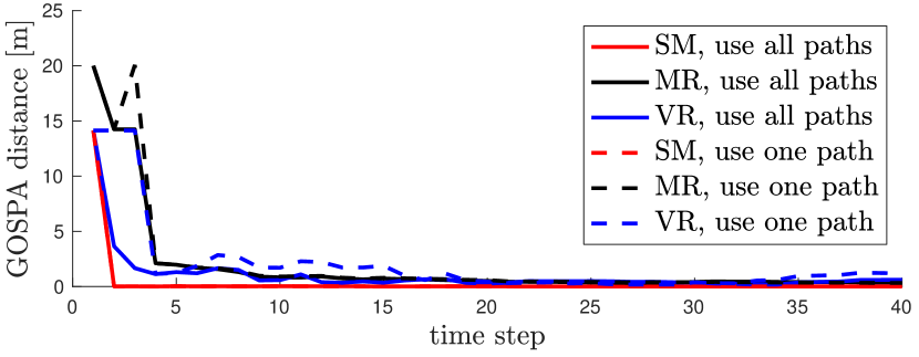
Figure 7: The comparison of mapping results between two algorithms for three landmark types.

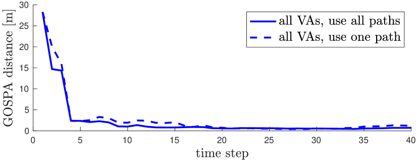
Figure 8: The comparison of overall mapping results between two algorithms.

Next, we study the performance of the proposed 5G SLAM scheme in vehicle state estimation. We add $[0.9,0.9,0,0.09,0,0,0.9]^{\mathrm{T}}$ bias to the initial state, use 2000 particles to represent the vehicle state, and obtain the mean absolute error (MAE) between the real vehicle state and the estimate vehicle state after the absolute error converges, as shown in Fig. 9. We observe that the absolute error converges after 2 time steps. The algorithm using all paths has better performance in positioning, as MAEs are lower.

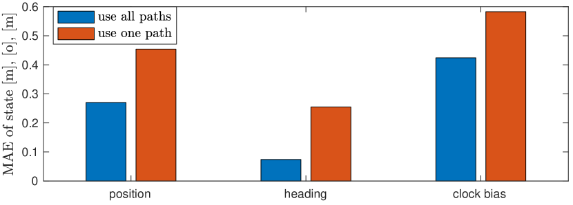
Figure 9: The comparison of vehicle state estimation results between two algorithms.

VI Conclusions

In this paper, we exploited diffuse multipath in 5G SLAM and proposed a novel 5G SLAM scheme, based on the PMBM filter, in which we have derived a new likelihood function for the filter that is able to utilize all 5G paths in every received signal cluster. Our results indicate that the proposed scheme can accurately estimate the number of landmarks, their types (i.e., roughness), and positions, and it outperforms the scheme using a single path in each signal cluster. The results also confirm the proposed method can handle mapping and vehicle state estimation simultaneously.

References

- [1] J. Nurmi, E.-S. Lohan, H. Wymeersch, G. Seco-Granados, and O. Nykänen, Multi-Technology Positioning. Springer, 2017.
- [2] H. Wymeersch, G. Seco-Granados, G. Destino, D. Dardari, and F. Tufvesson, “5G mmWave positioning for vehicular networks,” IEEE Wireless Communications, vol. 24, no. 6, pp. 80–86, 2017.
- [3] Y. Bar-Shalom, Tracking and Data Association. Academic Press Professional, Inc., 1987.
- [4] M. R. Akdeniz, Y. Liu, M. K. Samimi, S. Sun, S. Rangan, T. S. Rappaport, and E. Erkip, “Millimeter wave channel modeling and cellular capacity evaluation,” IEEE Journal on Selected Areas in Communications, vol. 32, no. 6, pp. 1164–1179, 2014.
- [5] K. Witrisal, P. Meissner, E. Leitinger, Y. Shen, C. Gustafson, F. Tufvesson, K. Haneda, D. Dardari, A. F. Molisch, A. Conti, et al., “High-accuracy localization for assisted living: 5G systems will turn multipath channels from foe to friend,” IEEE Signal Processing Magazine, vol. 33, no. 2, pp. 59–70, 2016.
- [6] A. Aubry, A. De Maio, G. Foglia, and D. Orlando, “Diffuse multipath exploitation for adaptive radar detection,” IEEE Transactions on Signal Processing, vol. 63, no. 5, pp. 1268–1281, 2015.
- [7] P. Setlur, T. Negishi, N. Devroye, and D. Erricolo, “Multipath exploitation in non-LOS urban synthetic aperture radar,” IEEE Journal of Selected Topics in Signal Processing, vol. 8, no. 1, pp. 137–152, 2013.
- [8] F. Wen, J. Kulmer, K. Witrisal, and H. Wymeersch, “5G positioning and mapping with diffuse multipath,” arXiv preprint arXiv:1912.08697, 2019.
- [9] R. Mendrzik, H. Wymeersch, and G. Bauch, “Joint localization and mapping through millimeter wave MIMO in 5G systems,” in IEEE Global Communications Conference (GLOBECOM), 2018, pp. 1–6.
- [10] H. Kim, H. Wymeersch, N. Garcia, G. Seco-Granados, and S. Kim, “5G mmWave vehicular tracking,” in 52nd IEEE Asilomar Conference on Signals, Systems, and Computers, 2018, pp. 541–547.
- [11] H. Kim, K. Granström, L. Gao, G. Battistelli, S. Kim, and H. Wymeersch, “5G mmWave cooperative positioning and mapping using multi-model PHD filter and map fusion,” IEEE Transactions on Wireless Communications, 2020.
- [12] R. W. Heath, N. Gonzalez-Prelcic, S. Rangan, W. Roh, and A. M. Sayeed, “An overview of signal processing techniques for millimeter wave MIMO systems,” IEEE Journal of Selected Topics in Signal Processing, vol. 10, no. 3, pp. 436–453, 2016.
- [13] Á. F. García-Fernández, J. L. Williams, K. Granström, and L. Svensson, “Poisson multi-Bernoulli mixture filter: direct derivation and implementation,” IEEE Transactions on Aerospace and Electronic Systems, vol. 54, no. 4, pp. 1883–1901, 2018.
- [14] J. L. Williams, “Marginal multi-Bernoulli filters: RFS derivation of MHT, JIPDA, and association-based MeMBer,” IEEE Transactions on Aerospace and Electronic Systems, vol. 51, no. 3, pp. 1664–1687, 2015.
- [15] M. Fatemi, K. Granström, L. Svensson, F. J. Ruiz, and L. Hammarstrand, “Poisson multi-Bernoulli mapping using Gibbs sampling,” IEEE Transactions on Signal Processing, vol. 65, no. 11, pp. 2814–2827, 2017.
- [16] R. P. Mahler, Advances in Statistical Multisource-Multitarget Information Fusion. Artech House, 2014.
- [17] R. P. Mahler, “Multitarget Bayes filtering via first-order multitarget moments,” IEEE Transactions on Aerospace and Electronic Systems, vol. 39, no. 4, pp. 1152–1178, 2003.
- [18] G. Li, “Multiple model Poisson multi-Bernoulli mixture filter for maneuvering targets,” arXiv preprint arXiv:1904.03716, 2019.
- [19] K. G. Murty, “Letter to the editor—an algorithm for ranking all the assignments in order of increasing cost,” Operations research, vol. 16, no. 3, pp. 682–687, 1968.
- [20] H. Wymeersch, “A simple method for 5G positioning and synchronization without line-of-sight,” arXiv preprint arXiv:1812.05417, 2018.
- [21] A. S. Rahmathullah, Á. F. García-Fernández, and L. Svensson, “Generalized optimal sub-pattern assignment metric,” in 20th IEEE International Conference on Information Fusion (Fusion), 2017, pp. 1–8.