A Benson-Type Algorithm for Bounded Convex Vector Optimization Problems with Vertex Selection

Abstract

We present an algorithm for approximately solving bounded convex vector optimization problems. The algorithm provides both an outer and an inner polyhedral approximation of the upper image. It is a modification of the primal algorithm presented by Löhne, Rudloff, and Ulus in 2014. There, vertices of an already known outer approximation are successively cut off to improve the approximation error. We propose a new and efficient selection rule for deciding which vertex to cut off. Numerical examples are provided which illustrate that this method may solve fewer scalar problems overall and therefore may be faster while achieving the same approximation quality.

90C29, 90C25, 90-08, 90C59

1 Introduction

There exists a variety of methods for (approximately) solving vector optimization problems. One of the most studied and best understood class is vector linear programming (VLP). There are numerous algorithms for VLP as surveyed by Ehrgott and Wiecek in [12]. These include the multiple objective simplex method, where the set of all efficient solutions is computed in the preimage space (or variable space) of the problem. In [3], an article from 1998, Benson proposes an approximation algorithm that computes the set of all efficient values by constructing a sequence of outer approximation polyhedra in the image space (or objective space). This is motivated by the idea that a decision maker tends to choose a solution based on objective function values rather than variable values, many efficient solutions may be mapped to the same efficient point and the dimension of the image space is typically much smaller than that of the preimage space. Although algorithms taking these considerations into account are frequently named after Benson, some of his ideas can be traced back to earlier works in different areas of research. In [8] from 1987, Dauer analyzes the image space in VLP and observes that the number of objectives is typically smaller than the number of variables. More than 15 years prior to Benson’s article the idea of approximation polyhedra had been used in global optimization, compare [43, 41, 40]. The ideas applied in these works can in turn be dated back to Cheney and Goldstein [5] from 1959 and Kelley [27] from 1960, who use cutting plane methods to solve convex programs. In [28] from 1992 Lassez and Lassez propose an algorithm for computing projections of polyhedra by successive refinements of approximations. Their approach can be viewed as a dual variant of the outer polyhedral approximation algorithm (also compare [10]). In [26] Kamenev formulates a framework for the approximation of convex bodies by polyhedra. In this article from 1992, the same ideas as in Benson’s algorithm are used already. An adequate solution concept for VLP based on the image space approach is presented in [23, 30]. Various modifications of Benson’s algorithm for VLP have since been developed, see e.g. [38, 39, 30, 10]. Improvements of these methods where fewer LPs have to be solved per iteration are presented in [21, 7].

Naturally, there has been effort to extend Benson’s algorithm from VLP to the more general class of vector convex programming (VCP) or convex vector optimization problems (CVOPs). Therefore solution concepts have been refined to adapt to approximate solutions, see the survey article by Ruzika and Wiecek [37]. However, a finite description of an approximate solution in terms of points and directions may not be possible for an unbounded problem, see [42]. For example, the epigraph of a parabola can not be approximated by a polyhedron, i.e. their Hausdorff distance is always infinite. In 2011, Ehrgott et al. [11] propose an approximation algorithm for bounded VCP motivated by Benson’s arguments for VLP. In [31] the authors develop an algorithm that generalizes and simplifies this approach. In particular, their method allows the use of (1) not necessarily differentiable objective and constraint functions, (2) more general ordering cones, and is simpler in the sense that (3) only one convex program has to be solved in every iteration throughout the algorithm. Moreover, a dual variant of the algorithm is provided.

In this paper we present a modification of the primal algorithm from [31]. It computes sequences of polyhedral inner and outer approximations of the upper image. In every iteration one vertex of the outer approximation is cut off to refine the approximation error. This requires solving one scalarization that is a convex program in which the vertex is passed as a parameter. In [31] this vertex is chosen arbitrarily. Here, we choose this vertex according to a specific heuristic which takes into consideration the Hausdorff distance between the current inner and outer approximations. This rule requires to solve convex quadratic subproblems. They differ from the scalarizations in the sense that the variables come from the (typically lower dimensional) image space of the vector program rather than the preimage space. Therefore, solving the subproblems is typically cheaper than solving a scalarization. Moreover, we show that not all subproblems have to be solved. Instead, optimality of solutions known from prior iterations can be verified by checking a single inequality. One advantage of this selection rule is that the approximation error is known at every time throughout the algorithm at no additional cost, whereas in [31] it is only known either at termination or after solving a number of scalarizations whose quantity typically increases with every iteration. We provide three examples comparing the method presented here with the original algorithm and illustrate its advantages. The first one is an academic example where the modification’s performance is not affected by a certain problem parameter, whereas the original algorithm’s runtime increases with the value of the parameter. In the second example we apply the method to the problem of regularization parameter tracking in machine learning. This has first been done by the authors of [14]. The last example concerns a real world problem from mechanical engineering. We use the algorithm presented here to analyze a truss design and find optimal distributions of loads among the trusses’ beam connections. In all examples fewer scalarizations need to be solved with the modification. This leads to (1) a decrease in runtime and (2) a smaller solution set while achieving the same approximation quality, which is preferred by decision makers as the amount of alternatives to choose from is less overwhelming.

This paper is organized as follows. In Section 2 the necessary notation is provided along with basic concepts. Section 3 is dedicated to the problem formulation and the theoretical background of VCP. A solution concept and scalarization techniques are presented. The vertex selection along with the modified version of the primal algorithm from [31] are presented in Section 4, correctness is proven, and a method for an efficient implementation is discussed. Numerical examples are provided in Section 5.

2 Preliminaries

Given a set $A\subseteq\mathbb{R}^{q}$, we denote by $\operatorname{cl}A$, $\operatorname{int}A$, $\operatorname{ri}A$, $\operatorname{conv}A$, $\operatorname{cone}A$ the closure, interior, relative interior, convex hull, and conic hull of $A$, respectively. We recall that every polyhedral set $A$ can be written as the intersection of finitely many closed halfspaces, i.e.

$$A=\bigcap_{i=1}^{\ell}\{x\in\mathbb{R}^{q}\mid w_{i}^{\mathsf{T}}x\geqslant\gamma_{i}\}$$ (1)

for $\ell\in\mathbb{N}$, $w_{i}\in\mathbb{R}^{q}$, $\gamma_{i}\in\mathbb{R}$ for all $i=1,\dots,\ell$. A set ${\{(w_{i},\gamma_{i})\mid i=1,\dots,\ell\}}$ of parameters fulfilling (1) is called $H$-representation of $A$. Equivalently, $A$ can be expressed as

$$A=\operatorname{conv}\{v^{1},\dots,v^{s}\}+\operatorname{cone}\{d^{1},\dots,d^{r}\}$$ (2)

for $s\in\mathbb{N}$, $r\in\mathbb{N}_{0}$, $v^{i}\in\mathbb{R}^{q}$, and $d^{i}\in\mathbb{R}^{q}\setminus\{0\}$, that is the Minkowski sum of the convex hull of finitely many points and the conic hull of finitely many directions. We set $\operatorname{cone}\emptyset=\{0\}$. The data $(\{v^{1},\dots,v^{s}\},\{d^{1},\dots,d^{r}\})$ from Equation (2) are called a $V$-representation of $A$. When expressing $A$ by $V$-representation, we will interchangeably write $A=\operatorname{conv}V+\operatorname{cone}D$ for matrices $V\in\mathbb{R}^{q\times s}$ and $D\in\mathbb{R}^{q\times r}$ where the columns of $V$ and $D$ are the $v^{i}$ and $d^{i}$ in (2), respectively. A pointed convex cone $C\subseteq\mathbb{R}^{q}$ induces a partial order $\leqslant_{C}$ on $\mathbb{R}^{q}$ by

$$x\leqslant_{C}y\text{ if and only if }y-x\in C.$$

The nonnegative orthant of $\mathbb{R}^{q}$ is denoted by $\mathbb{R}^{q}_{+}$ and induces the natural (or component-wise) order on $\mathbb{R}^{q}$ which we denote by $\leqslant$ rather than by $\leqslant_{\mathbb{R}^{q}_{+}}$. The dual cone $C^{+}$ of $C$ is the set $C^{+}:=\{y\in\mathbb{R}^{q}\mid\forall x\in C\colon y^{\mathsf{T}}x\geqslant 0\}$. We call $C$ polyhedral if there is a matrix ${D\in\mathbb{R}^{q\times r}}$, such that ${C=\operatorname{cone}D:=\{D\mu\mid\mu\geqslant 0\}}$. We summarize some important facts about the set $C=\operatorname{cone}D$ [see 25, 18]:

1. There is a matrix $Z\in\mathbb{R}^{q\times\ell}$ such that $C=\{x\in\mathbb{R}^{q}\mid Z^{\mathsf{T}}x\geqslant 0\}$. In particular, $C^{+}=\operatorname{cone}Z$.

2. $C=(C^{+})^{+}$.

3. $C$ is pointed if and only if $\operatorname{rank}Z=q$.

4. $\operatorname{int}C=\{x\in\mathbb{R}^{q}\mid Z^{\mathsf{T}}x>0\}$.

From (1) we obtain that $x\leqslant_{C}y$ if and only if $Z^{\mathsf{T}}x\leqslant Z^{\mathsf{T}}y$ for $x,y\in\mathbb{R}^{q}$. For a set ${A\subseteq\mathbb{R}^{q}}$ and a pointed convex cone $C\subseteq\mathbb{R}^{q}$ an element $x\in A$ is called $C$-minimal if $(\{x\}-C\setminus\{0\})\cap A=\emptyset$ and, if $\operatorname{int}C\neq\emptyset$, $x\in A$ is called weakly $C$-minimal if ${(\{x\}-\operatorname{int}C)\cap A=\emptyset}$. Given nonempty sets $A,B\subseteq\mathbb{R}^{q}$ we denote by  $d_{\mathsf{H}}(A,B)$ the Hausdorff distance between $A$ and $B$ which is defined as

$$d_{\mathsf{H}}(A,B):=\max\left\{\adjustlimits{\sup}_{a\in A}{\inf}_{b\in B}\left\lVert{a-b}\right\rVert,\adjustlimits{\sup}_{b\in B}{\inf}_{a\in A}\left\lVert{a-b}\right\rVert\right\},$$ (3)

where $\left\lVert{\cdot}\right\rVert$ denotes the euclidean norm in $\mathbb{R}^{q}$. It is well known that $d_{\mathsf{H}}(\cdot,\cdot)$ defines a metric on the space of nonempty compact subsets of $\mathbb{R}^{q}$. The Hausdorff distance between arbitrary sets may be infinite. It holds true, however, that for nonempty compact sets ${A,B\subseteq\mathbb{R}^{q}}$ and convex cones $C^{1},C^{2}\subseteq\mathbb{R}^{q}$ the value of $d_{\mathsf{H}}(A+C^{1},B+C^{2})$ is finite if and only if $\operatorname{cl}C^{1}=\operatorname{cl}C^{2}$. Moreover, if $A$ and $B$ are polyhedra with the same pointed recession cone one has

$$d_{\mathsf{H}}(A,B)=\max\left\{\adjustlimits{\max}_{a\in\operatorname{vert}A}{\min}_{b\in B}\left\lVert{a-b}\right\rVert,\adjustlimits{\max}_{b\in\operatorname{vert}B}{\min}_{a\in A}\left\lVert{a-b}\right\rVert\right\},$$ (4)

where $\operatorname{vert}A$ and $\operatorname{vert}B$ denote the set of vertices of $A$ and $B$, respectively. For proofs of the above statements we refer the reader to [1]. The domain of an extended real-valued function $g\colon\mathbb{R}^{q}\to\mathbb{R}\cup\{\infty\}$ is written as $\operatorname{dom}g$. Given a function $f\colon\mathbb{R}^{n}\to\mathbb{R}^{q}$ and a pointed convex cone $C\subseteq\mathbb{R}^{q}$, $f$ is called $C$-convex if for $x,y\in\mathbb{R}^{n}$ and $\lambda\in[0,1]$ it holds

$$f(\lambda x+(1-\lambda)y)\leqslant_{C}\lambda f(x)+(1-\lambda)f(y).$$ (5)

3 Vector Convex Programs

A vector convex program (VCP) is given as

$$\min\;F(x)\;\text{w.r.t}\;\leqslant_{C}\;\text{s.t.}\;g(x)\leqslant 0,$$ (P)

where $F\colon X\to\mathbb{R}^{q}$ is a $C$-convex function, in particular, $X\subseteq\mathbb{R}^{n}$ is a convex set and ${C\subseteq\mathbb{R}^{q}}$ is a pointed convex cone. The constraint function is given as  ${g=(g_{1},\dots,g_{m})^{\mathsf{T}}}$, where for every $i=1,\dots,m$ the component  ${g_{i}\colon\mathbb{R}^{n}\to\mathbb{R}\cup\{\infty\}}$ is a convex function. We set $\operatorname{dom}g:=\bigcap_{i=1}^{m}\operatorname{dom}g_{i}$. Hence, $g$ is an $\mathbb{R}^{m}_{+}$-convex (component-wise convex) function. The feasible set of (P) is denoted by $S$, i.e. ${S=\{x\in X\mid g(x)\leqslant 0\}}$ and its image under $F$ by $F[S]$. Throughout this article we make the following additional assumptions about (P):

Assumptions.

1. The objective function $F\colon X\to\mathbb{R}^{q}$ is continuous.

2. The constraint functions $g_{i}\colon\mathbb{R}^{n}\to\mathbb{R}\cup\{\infty\}$, $i=1,\dots,m$, are proper, lower semi-continuous, and their domains are relatively open.

3. $\bigcap_{i=1}^{m}\operatorname{ri}\{x\in X\mid g_{i}(x)\leqslant 0\}\neq\emptyset$

4. The feasible region $S$ of (P) is bounded.

5. The cone $C$ has nonempty interior and is given as ${C=\{x\in\mathbb{R}^{q}\mid Z^{\mathsf{T}}x\geqslant 0\}}$.

Definition 3.1.

Given a VCP (P) the set

$$\mathcal{P}:=\operatorname{cl}(F[S]+C)$$ (6)

is called the upper image of (P). We say that (P) is bounded if there exists some $y\in\mathbb{R}^{q}$ such that $\mathcal{P}\subseteq\{y\}+C$.

Clearly, $\mathcal{P}$ is a closed and convex set.

Definition 3.2.

A point $x\in S$ is called a (weak) minimizer for (P) if $F(x)$ is a (weakly) $C$-minimal element of $F[S]$. A nonempty subset $\mathcal{X}\subseteq S$ is called an infimizer of (P) if $\operatorname{cl}\operatorname{conv}(F[\mathcal{X}]+C)=\mathcal{P}$. An infimizer $\mathcal{X}\subseteq S$ is called a (weak) solution of (P) if it consists of (weak) minimizers only.

This type of solution concept is introduced and studied in [23] where Definition 3.2 is called a mild solution. It has been adapted to the case of VLP in [30] where one is interested in finite solutions consisting of minimal points and directions. The solution concept is extended to finite approximate solutions for bounded VCPs in [31].

Definition 3.3.

A nonempty finite subset $\mathcal{X}\subseteq S$ is called an $\varepsilon$-infimizer for a bounded problem (P) if

$$d_{\mathsf{H}}(\operatorname{conv}F[\mathcal{X}]+C,\mathcal{P})\leqslant\varepsilon.$$ (7)

A finite $\varepsilon$-infimizer $\mathcal{X}\subseteq S$ is called a (weak) $\varepsilon$-solution of (P) if it consists of (weak) minimizers only.

An illustration of the definition can be seen in Figure 1.

 

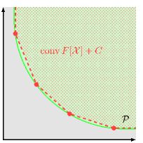
Figure 1: Illustration of an $\varepsilon$-solution ${\mathcal{X}}\subseteq S$ (see Definition 3.3). The four points of $F[\mathcal{X}]$ are $C$-minimal in $\mathcal{P}$, hence ${\mathcal{X}}$ is a set of minimizers. The Hausdorff distance between ${\operatorname{conv}F[\mathcal{X}]+C}$ and $\mathcal{P}$ is $\varepsilon$.

Remark 3.4.

The original definition of an $\varepsilon$-infimizer given in [31] is a different one. There, condition (7) is replaced by

$$\operatorname{conv}F[\mathcal{X}]+C-\varepsilon\{c\}\supseteq\mathcal{P}$$ (8)

for some fixed direction $c\in\operatorname{int}C$. Clearly, if (8) holds one has

$$d_{\mathsf{H}}(\operatorname{conv}F[\mathcal{X}]+C,\mathcal{P})\leqslant\varepsilon\left\lVert c\right\rVert.$$ (9)

Since $C$ is a cone we could choose $c\in\operatorname{int}C$ such that $\left\lVert c\right\rVert=1$. Then (8) implies that  $\mathcal{X}$ is an $\varepsilon$-infimizer in the sense of Definition 3.3. The converse is also true up to a constant:

Proposition 3.5.

Let $\mathcal{X}\subseteq S$ be an $\varepsilon$-infimizer for a bounded problem (P) according to Definition 3.3 and let $C$ be closed. Then for every $c\in\operatorname{int}{C}$ with $\left\lVert{c}\right\rVert=1$ and every ${k\geqslant(\min\{w^{\mathsf{T}}c\mid w\in C^{+},\left\lVert{w}\right\rVert=1\})^{-1}}$ it holds that

$$\operatorname{conv}{F[\mathcal{X}]}+C-k\varepsilon\{c\}\supseteq\mathcal{P}.$$

Proof.

Since $\operatorname{conv}F[\mathcal{X}]+C$ is non-empty, closed and convex, it can be written as an intersection of closed halfspaces [see 35, Theorem 18.8], i.e.

$$\operatorname{conv}F[\mathcal{X}]+C=\bigcap_{i\in I}\{y\in\mathbb{R}^{q}\mid w_{i}^{\mathsf{T}}y\geqslant\gamma_{i}\}$$

for $w_{i}\in\mathbb{R}^{q}\setminus\{0\}$, $\left\lVert{w_{i}}\right\rVert=1$, $\gamma_{i}\in\mathbb{R}$, and some index set $I$. Because the recession cone of $\operatorname{conv}F[\mathcal{X}]+C$ is $C$, we have $w_{i}\in C^{+}$ for all $i\in I$. Therefore ${w_{i}^{\mathsf{T}}c>0}$ for all $i\in I$ [4, p. 64] and ${k_{p}:=\inf\{t\geqslant 1\mid p+t\varepsilon c\in\operatorname{conv}F[\mathcal{X}]+C\}}$ exists for all ${p\in\mathcal{P}}$. It remains to show that ${(\min\{w^{\mathsf{T}}c\mid w\in C^{+},\left\lVert{w}\right\rVert=1\})^{-1}\geqslant\sup\{k_{p}\mid p\in\mathcal{P}\}}$. Therefore, let $p\in\mathcal{P}$ such that $k_{p}>1$. If no such $p$ exists we are done, because ${(\min\{w^{\mathsf{T}}c\mid w\in C^{+},\left\lVert{w}\right\rVert=1\})^{-1}\in[1,\infty)}$. Otherwise there exists $j\in I$ such that $w_{j}^{\mathsf{T}}(p+k_{p}\varepsilon c)=\gamma_{j}$. Denote by $d$ the euclidean distance from $p$ to the hyperplane defined by $(w_{j},\gamma_{j})$, i.e. $d=\gamma_{j}-w_{j}^{\mathsf{T}}p$. Then we obtain $k_{p}=d(\varepsilon w_{j}^{\mathsf{T}}c)^{-1}$. Next, observe that $d\leqslant\varepsilon$: Because $d_{\mathsf{H}}(\operatorname{conv}F[\mathcal{X}]+C,\mathcal{P})\leqslant\varepsilon$, there exists a direction $u\in\mathbb{R}^{q}$ with $\left\lVert{u}\right\rVert\leqslant\varepsilon$ such that $p+u\in\operatorname{conv}F[\mathcal{X}]+C$. Assuming ${d>\varepsilon}$ yields ${w_{j}^{\mathsf{T}}(p+\left\lVert{u}\right\rVert w_{j})<\gamma_{j}\leqslant w_{j}^{\mathsf{T}}(p+u)}$. Therefore $w_{j}^{\mathsf{T}}u>\left\lVert{u}\right\rVert$, which is a contradiction to the Cauchy-Schwarz inequality. Hence, we have

$$k_{p}\leqslant\frac{1}{w_{j}^{\mathsf{T}}c}\leqslant\frac{1}{\min_{i\in I}w_{i}^{\mathsf{T}}c}\leqslant\frac{1}{\min_{w\in C^{+},\left\lVert{w}\right\rVert=1}w^{\mathsf{T}}c}$$

which completes the proof. ∎

Note that the closedness of $C$ can be omitted if the inequality in the statement is turned strict. We use Definition 3.3 in this article, because it has the advantage of being independent of any directions.

Assumptions (A1), (A2), (A4), and (A5) imply that (P) is bounded: By [35, Theorem 7.1] the sets $\{x\in X\mid g_{i}(x)\leqslant 0\}$ are closed for all $i=1,\dots,m$ by lower semi-continuity. Therefore $S=\bigcap_{i=1}^{m}\{x\in X\mid g_{i}(x)\leqslant 0\}$ is closed and compact by (A4). Now, since $F$ is continuous by (A1), $F[S]$ is compact as well. Finally, because ${\operatorname{int}C\neq\emptyset}$, there is some $y\in\mathbb{R}^{q}$ such that $\mathcal{P}\subseteq\{y\}+C$. Moreover, Assumption (A2) implies that [see 35, Corollary 7.6.1] ${\operatorname{ri}\{x\in X\mid g_{i}(x)\leqslant 0\}=\{x\in X\mid g_{i}(x)<0\}}$ for $i=1,\dots,m$ and Assumption (A3) implies that [see 35, Theorem 6.5]

$$\bigcap_{i=1}^{m}\operatorname{ri}\{x\in X\mid g_{i}(x)\leqslant 0\}=\operatorname{ri}\bigcap_{i=1}^{m}\{x\in X\mid g_{i}(x)\leqslant 0\}.$$

Therefore it holds

$$\operatorname{ri}S=\{x\in X\mid g(x)<0\}$$ (10)

and the set is nonempty.

For some parameter $w\in\mathbb{R}^{q}$ the problem

$$\min w^{\mathsf{T}}F(x) w$$ (P₁())

s.t. $$g(x)\leqslant 0$$

is the well-known weighted sum scalarization of (P). By Assumption (A1) and compactness of $S$ an optimal solution of (P₁($w$)) exists for every $w\in\mathbb{R}^{q}$. The following is a common result, see e.g. [24, 29].

Proposition 3.6.

Let $w\in C^{+}\setminus\{0\}$. An optimal solution $x^{w}$ of (P₁($w$)) is a weak minimizer of (P).

We consider another scalarization [see e.g. 31, 21] that can be stated as

$$\min z v,c$$ (P₂())

s.t. $$g(x)\leqslant 0,$$

$$Z^{\mathsf{T}}(F(x)-v-zc)\leqslant 0,$$

with a parameter $v\in\mathbb{R}^{q}$, that does typically not belong to $\mathcal{P}$, and a direction $c\in\mathbb{R}^{q}$. The Lagrangian dual problem of (P₂($v,c$)) is given as

$$\max \inf_{x\in X\cap\operatorname{dom}g}\left\{u^{\mathsf{T}}g(x)+w^{\mathsf{T}}F(x)\right\}-w^{\mathsf{T}}v v,c$$ (D₂())

s.t. $$u\geqslant 0,$$

$$w^{\mathsf{T}}c=1,$$

$$w\in C^{+}.$$

The following primal-dual relationship between (P₂($v,c$)) and (D₂($v,c$)) has been established in [31, Proposition 4.4] in a similar form. The proof is presented here due to a flaw in the original work claiming that the feasible region of (P₂($v,c$)) is compact.

Proposition 3.7.

Let Assumptions (A1) – (A5) hold and let $p\in\operatorname{int}\mathcal{P}$. Then for every ${v\in\mathbb{R}^{q}\setminus\mathcal{P}}$ and $c:=p-v$, solutions $(x^{*},z^{*})$ and $(u^{*},w^{*})$ to (P₂($v,c$)) and (D₂($v,c$)), respectively, exist and their optimal values coincide.

Proof.

By [35, Corollary 6.6.2] we have $\operatorname{int}\mathcal{P}=\operatorname{ri}F[S]+\operatorname{int}C$. Assumption (A1) and [35, Theorem 6.6] yield that $\operatorname{ri}F[S]\subseteq F[\operatorname{ri}S]$. Therefore we can write $p\in\operatorname{int}\mathcal{P}$ as ${p=F(x)+\bar{c}}$ for some $x\in\operatorname{ri}S$ and $\bar{c}\in\operatorname{int}C$. From Assumption (A5) we conclude

$$Z^{\mathsf{T}}(F(x)-v-c)=Z^{\mathsf{T}}(F(x)-p)=-Z^{\mathsf{T}}\bar{c}<0. *$$ ()

This implies that $(x,1)$ is feasible for (P₂($v,c$)). Since $v\notin\mathcal{P}$, the second constraint of (P₂($v,c$)) is violated whenever $z\leqslant 0$. From Assumptions (A1), (A2), and (A4) it follows that the set

$$\{(x,z)\in\mathbb{R}^{n+1}\mid g(x)\leqslant 0,Z^{\mathsf{T}}(F(x)-v-zc)\leqslant 0,z\leqslant 1\}$$

is compact and nonempty. Thus there exists an optimal solution $(x^{*},z^{*})$ of (P₂($v,c$)) by the extreme value theorem and one has $0\leqslant z^{*}\leqslant 1$. Next, observe that $(x,1)$ is also strictly feasible for (P₂($v,c$)) by Equations (10) and ($*$ ‣ 3). This is the well-known Slater’s constraint qualification. Consequently strong duality holds, i.e. there exists an optimal solution $(u^{*},w^{*})$ of (D₂($v,c$)) and the optimal values coincide. ∎

Similar to Proposition 3.6 we obtain weak minimizers of (P) from solutions of (P₂($v,c$)). The following is Proposition 4.5 from [31].

Proposition 3.8.

Let $(x^{*},z^{*})$ be a solution to (P₂($v,c$)). Then $x^{*}$ is a weak minimizer of (P) and $y:=v+z^{*}c$ is a weakly $C$-minimal element of $\mathcal{P}$.

4 An Algorithm for Bounded VCPs with Vertex Selection

In this section we present an algorithm for computing a weak $\varepsilon$-solution for Problem (P). The algorithm computes a shrinking sequence $(\mathcal{O}^{k})$ of polyhedral outer approximations and a growing sequence $(\mathcal{I}^{k})$ of polyhedral inner approximations of the upper image $\mathcal{P}$, i.e. one has

$$\mathcal{O}^{0}\supseteq\mathcal{O}^{1}\supseteq\dots\supseteq\mathcal{P}\supseteq\dots\supseteq\mathcal{I}^{1}\supseteq\mathcal{I}^{0}.$$ (11)

This is achieved by iteratively cutting off vertices $v$ of $\mathcal{O}^{k}$ while introducing new halfspaces. The algorithm is a modification of the primal approximation algorithm presented in [31]. The difference lies in the way the approximations are updated. While in [31] there is no rule stated how to choose the next vertex, we employ a vertex selection that takes into account $d_{\mathsf{H}}(\mathcal{O}^{k},\mathcal{I}^{k})$. Therefore $d_{\mathsf{H}}(\mathcal{O}^{k},\mathcal{I}^{k})$ is computed in each iteration by solving certain convex quadratic subproblems. We formulate Corollary 4.4 to show that the vertex selection can be performed efficiently. The algorithm consists of two parts, an initialization phase and an update phase, which we will explain in detail below. Correctness is shown in Theorem 4.3.

Initialization.

In the initialization phase an initial outer approximation $\mathcal{O}^{0}$ and an initial inner approximation $\mathcal{I}^{0}$ of $\mathcal{P}$ are computed. To obtain $\mathcal{O}^{0}$, (P₁($z^{j}$)) is solved for every column $z^{j}$ of $Z$. Solutions $x^{j}$ are weak minimizers of (P) according to Proposition 3.6 and give rise to the following hyperplanes that support $\mathcal{P}$ at $F(x^{j})$:

$$\mathcal{H}_{j}:=\{y\in\mathbb{R}^{q}\mid z^{j\mathsf{T}}y=z^{j\mathsf{T}}F(x^{j})\}.$$ (12)

Thus, we can define $\mathcal{O}^{0}$ as the intersection of all halfspaces $\mathcal{H}_{j}^{+}$ that are defined by $\mathcal{H}_{j}$, i.e.

$$\mathcal{O}^{0}:=\bigcap_{j=1}^{\ell}\mathcal{H}_{j}^{+}=\bigcap_{j=1}^{\ell}\{y\in\mathbb{R}^{q}\mid z^{j\mathsf{T}}y\geqslant z^{j\mathsf{T}}F(x^{j})\}.$$ (13)

Note that $\mathcal{O}^{0}$ has at least one vertex, because (P) is bounded and $C$ is an ordering cone, in particular pointed. An initial inner approximation $\mathcal{I}^{0}$ is readily available at no additional cost by setting

$$\mathcal{I}^{0}:=\operatorname{conv}\{F(x^{j})\mid j=1,\dots,\ell\}+C.$$ (14)

Update Step.

During the update phase the current approximations are refined. In order to do so, supporting hyperplanes to the upper image are computed from solutions of (P₂($v,c$)) and (D₂($v,c$)) according to the following proposition [see 31, Proposition 4.7].

Proposition 4.1.

Let $(x^{*},z^{*})$ and $(u^{*},w^{*})$ be solutions of (P₂($v,c$)) and (D₂($v,c$)), respectively. Then the hyperplane

$$\mathcal{H}:=\{y\in\mathbb{R}^{q}\mid w^{*\mathsf{T}}y=w^{*\mathsf{T}}v+z^{*}\}$$

is a supporting hyperplane of $\mathcal{P}$ at $y^{*}:=v+z^{*}c$.

In iteration $k$ the input parameters for P₂($v,c$) are chosen by means of the following vertex selection procedure (VS).

Vertex Selection.

For every $s\in\operatorname{vert}\mathcal{O}^{k}$ the euclidean distance to $\mathcal{I}^{k}$ is computed by solving

$$\min \left\lVert{p-s}\right\rVert^{2} s,\mathcal{I}^{k}$$ (QP())

s.t. $$p\in\mathcal{I}^{k}.$$

Note that (QP($s,\mathcal{I}^{k}$)) lives in the image space of (P) and is convex quadratic. Next we consider the following bilevel optimization problem

$$\max \left\lVert{p^{*}-s}\right\rVert \mathcal{O}^{k},\mathcal{I}^{k}$$ (VS())

s.t. $$s\in\operatorname{vert}\mathcal{O}^{k}$$

$$p^{*}\;\text{solves}\;\eqref{QP}.$$

A solution to (VS($\mathcal{O}^{k},\mathcal{I}^{k}$)) is a vertex of $\mathcal{O}^{k}$ that yields the shortest distance to the current inner approximation. Since $\mathcal{O}^{k}\supseteq\mathcal{I}^{k}$ by construction, we obtain the Hausdorff distance $d_{\mathsf{H}}(\mathcal{O}^{k},\mathcal{I}^{k})$ easily from a solution of (VS($\mathcal{O}^{k},\mathcal{I}^{k}$)) as explained in the next corollary.

Corollary 4.2.

Let $\mathcal{O},\mathcal{I}\subseteq\mathbb{R}^{q}$ be polyhedra with the same pointed recession cone and ${\mathcal{O}\supseteq\mathcal{I}}$. Further let $(s^{*},p^{*})$ be a solution of (VS($\mathcal{O}$,$\mathcal{I}$)). Then

$$d_{\mathsf{H}}(\mathcal{O},\mathcal{I})=\left\lVert{p^{*}-s^{*}}\right\rVert.$$

Proof.

As $\mathcal{O}\supseteq\mathcal{I}$ and by Equation (4), the maximum in the definition of $d_{\mathsf{H}}$ is attained as

$$\adjustlimits{\max}_{s\in\operatorname{vert}\mathcal{O}}{\min}_{p\in\mathcal{I}}\left\lVert{p-s}\right\rVert.$$

Since squaring the norm in the objective function of (QP) does not change the solution, we get

$$d_{\mathsf{H}}(\mathcal{O},\mathcal{I}) =\adjustlimits{\max}_{s\in\operatorname{vert}\mathcal{O}}{\min}_{p\in\mathcal{I}}\left\lVert{p-s}\right\rVert$$

$$=\max_{s\in\operatorname{vert}\mathcal{O}}\left\{\left\lVert{p^{*}-s}\right\rVert\mid p^{*}\;\text{is a solution of (QP($s,\mathcal{I}$))}\right\}$$

$$=\left\lVert{p^{*}-s^{*}}\right\rVert.\qed$$

Note that solving (VS($\mathcal{O}^{k},\mathcal{I}^{k}$)) amounts to solving (QP($s,\mathcal{I}^{k}$)) for every vertex $s$ of $\mathcal{O}^{k}$ and taking a maximum over a finite set. If $d_{\mathsf{H}}(\mathcal{O}^{k},\mathcal{I}^{k})\leqslant\varepsilon$, then $d_{\mathsf{H}}(\mathcal{O}^{k},\mathcal{P})\leqslant\varepsilon$ and $d_{\mathsf{H}}(\mathcal{P},\mathcal{I}^{k})\leqslant\varepsilon$ follow immediately from the fact that $\mathcal{O}^{k}\supseteq\mathcal{P}\supseteq\mathcal{I}^{k}$. In this case a weak $\varepsilon$-solution $\mathcal{X}$ to (P) is returned. Otherwise we set $v:=s^{*}$ and ${c:=p^{*}-s^{*}}$ and solve P₂($v,c$). Thereby we obtain a supporting hyperplane $\mathcal{H}$ of  $\mathcal{P}$ according to Proposition 4.1 and set

$$\mathcal{O}^{k+1} =\mathcal{O}^{k}\cap\mathcal{H}^{+},$$ (15)

$$\mathcal{I}^{k+1} =\operatorname{cl}\operatorname{conv}\left(\mathcal{I}^{k}\cup\{F(x^{*})\}\right),$$

where $x^{*}$ solves (P₂($v,c$)). Also, $x^{*}$ is appended to the solution set $\mathcal{X}$. Note, that the closure in Equation (15) is necessary, because we are dealing with unbounded sets. However, $\mathcal{I}^{k+1}$ does not have to be computed explicitly as we are only interested in its vertices. Pseudocode is presented in Algorithm 1 and one iteration of the algorithm is illustrated in Figure 2.

Data: Problem (P), accuracy $\varepsilon>0$, max. no. of iterations $K$

Result: Weak $\varepsilon$-solution $\mathcal{X}$ of (P), vertices $\mathcal{O}$/$\mathcal{I}$ of an outer/inner approximation of $\mathcal{P}$ or max. no. of iterations exceeded

1 Compute a solution $x^{j}$ to (P₁($z^{j}$)) for $j=1,\dots,\ell$

2 $\mathcal{X}\leftarrow\{x^{j}\mid j=1,\dots,\ell\}$

3 Compute an outer approximation $\mathcal{O}^{0}$ according to (13)

4 Compute an inner approximation $\mathcal{I}^{0}$ according to (14)

5 $k\leftarrow 0$, $d_{\mathsf{H}}\leftarrow\infty$

6 repeat

7       Compute a solution $(s,p)$ to (VS($\mathcal{O}^{k},\mathcal{I}^{k}$))

8       $d_{\mathsf{H}}\leftarrow\left\lVert{p-s}\right\rVert$

9       if $d_{\mathsf{H}}>\varepsilon$ then

10             $v\leftarrow s$, $c\leftarrow p-s$

11             Compute solutions $(x,z)$/$(u,w)$ to (P₂($v,c$))/(D₂($v,c$))

12             $\mathcal{X}\leftarrow\mathcal{X}\cup\{x\}$

13             $\mathcal{O}^{k+1}\leftarrow\mathcal{O}^{k}\cap\{y\in\mathbb{R}^{q}\mid w^{\mathsf{T}}y\geqslant w^{\mathsf{T}}v+z\}$

14             $\mathcal{I}^{k+1}\leftarrow\operatorname{cl}\operatorname{conv}(\mathcal{I}^{k}\cup\{F(x)\})$

15             $k\leftarrow k+1$

16            

17      

18until $d_{\mathsf{H}}\leqslant\varepsilon$ or $k=K$

19$\mathcal{O}\leftarrow\operatorname{vert}\mathcal{O}^{k}$

20 $\mathcal{I}\leftarrow\operatorname{vert}\mathcal{I}^{k}$

return $\mathcal{X}$, $\mathcal{O}$, $\mathcal{I}$

Algorithm 1 A Benson-type Algorithm with Vertex Selection for (P)

 

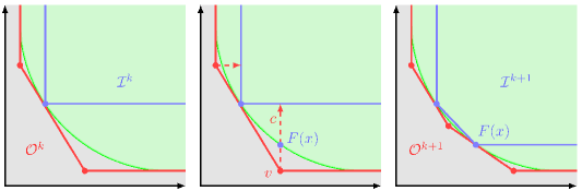
Figure 2: Left: Outer (red) and inner (blue) approximations of $\mathcal{P}$ after iteration $k$. Center: The vertex $v$ and direction $c$ are obtained by the vertex selection. The point $F(x)$ is obtained by solving (P₂($v,c$)). Right: The updated outer and inner approximations after cutting off $v$ and adding $F(x)$ as a vertex to $\mathcal{I}^{k}$.

Theorem 4.3.

Under Assumptions (A1) – (A5) Algorithm 1 is correct, i.e. if it terminates with $k<K$ it returns a weak $\varepsilon$-solution of (P).

Proof.

Optimal solutions to (P₁($z^{j}$)) exist for all $j=1,\dots,\ell$ by Assumptions (A1), (A2), and (A4). Therefore line 1 is valid and the set $\mathcal{X}$ initialized in line 2 is nonempty. Proposition 3.6 states that $\mathcal{X}$ only contains weak minimizers of (P) and implies that the vertices of $\mathcal{I}^{0}$ are weakly $C$-minimal elements of $\mathcal{P}$. Because $C$ is a pointed cone, the set $\mathcal{O}^{0}$ has at least one vertex. Therefore the problem (VS($\mathcal{O}^{0},\mathcal{I}^{0}$)) has a solution. Optimal solutions to (P₂($v,c$)) and (D₂($v,c$)) exist according to Proposition 3.7. By Proposition 3.8 a weak minimizer of (P) is added to $\mathcal{X}$ in line 12 and $\mathcal{I}^{k}$ is updated with a new vertex that is weakly $C$-minimal in $\mathcal{P}$. Now, $\mathcal{I}^{k+1}\subseteq\mathcal{P}$, because it is the generalized convex hull of finitely many weakly $C$-minimal points and directions of $\mathcal{P}$. Moreover, as the hyperplane $\{y\in\mathbb{R}^{q}\mid w^{\mathsf{T}}y=w^{\mathsf{T}}v+z\}$ supports $\mathcal{P}$ in $v+zc$, the set $\mathcal{O}^{k+1}$ in line 13 is nonempty, has a vertex, and satisfies $\mathcal{O}^{k+1}\supseteq\mathcal{P}$. Note that by Corollary 4.2, $d_{\mathsf{H}}$ defined in line 8 is the Hausdorff distance between the current approximations $\mathcal{O}^{k}$ and $\mathcal{I}^{k}$. Therefore, assuming termination with $k<K$, the algorithm terminates if the Hausdorff distance between the current outer and inner approximation of $\mathcal{P}$ is less than or equal to the error margin $\varepsilon$. Assume this is the case after $\kappa$ iterations. We must show that $\mathcal{X}$ is a weak $\varepsilon$-solution of (P). Clearly, $\mathcal{X}$ is finite and, by Propositions 3.6 and 3.8, it consists of weak minimizers only. Moreover we have ${d_{\mathsf{H}}(\mathcal{O}^{\kappa},\mathcal{I}^{\kappa})\leqslant\varepsilon}$ and therefore $d_{\mathsf{H}}(\mathcal{P},\mathcal{I}^{\kappa})\leqslant\varepsilon$. Finally, due to its construction, $\mathcal{I}^{\kappa}$ can be written as ${\mathcal{I}^{\kappa}=\operatorname{conv}F[\mathcal{X}]+C}$. Hence, $\mathcal{X}$ fulfills the definition of a weak $\varepsilon$-solution which completes the proof. ∎

Efficient Implementation of the Vertex Selection.

So far, the main drawback of the vertex selection is that it requires (QP($s,\mathcal{I}^{k}$)) to be solved for every $s\in\operatorname{vert}\mathcal{O}^{k}$. In order to make VS efficient, we make the following observation about the input parameters: From one iteration to the next, the inner approximation only changes by introducing one new vertex. Therefore the solutions of (QP($s,\mathcal{I}^{k}$)) and  (QP($s,\mathcal{I}^{k+1}$)) may be identical. We can exploit this structure by checking a single inequality to determine whether, for a given vertex $s$ of $\mathcal{O}^{k}$, we have to solve (QP($s,\mathcal{I}^{k}$)). The following result captures this idea.

Corollary 4.4.

Let the iteration be $k+1$ in Algorithm 1. Let $s$ be a vertex of both $\mathcal{O}^{k}$ and $\mathcal{O}^{k+1}$, let $p^{*}$ be a solution to (QP($s,\mathcal{I}^{k}$)) and $F(x)$ such that ${\mathcal{I}^{k+1}=\operatorname{cl}\operatorname{conv}(\mathcal{I}^{k}\cup\{F(x)\})}$. Then the following are equivalent:

1. $p^{*}$ is a solution to (QP($s,\mathcal{I}^{k+1}$)),

2. $(p^{*}-s)^{\mathsf{T}}(F(x)-p^{*})\geqslant 0$.

Proof.

This is a straightforward consequence of convexity and a standard result in convex optimization. Given a convex optimization problem with differentiable objective function $f$ and feasible region $S$ the following are equivalent, see [4, Section 4.2.3.]:

1. $p^{*}\in S$ is a solution,

2. $\nabla f(p^{*})^{\mathsf{T}}(p-p^{*})\geqslant 0$ for all $p\in S$.

Together with $\nabla\left[\left\lVert{p^{*}-s}\right\rVert^{2}\right]=2(p^{*}-s)$, (i) is equivalent to

$$(p^{*}-s)^{\mathsf{T}}(p-p^{*})\geqslant 0\;\text{for all}\;p\in\mathcal{I}^{k+1}.$$

This inequality holds in particular for $p=F(x)\in\mathcal{I}^{k+1}$. Therefore (i) implies (ii). On the other hand, assume that (ii) holds and $p^{*}$ is not a solution to (QP($s,\mathcal{I}^{k+1}$)). Then, as $p^{*}$ solves (QP($s,\mathcal{I}^{k}$)), there must exist some $\bar{p}\in\mathcal{I}^{k+1}$, such that

$$(p^{*}-s)^{\mathsf{T}}(\bar{p}-p^{*})<0.$$

By the definition of $\mathcal{I}^{k+1}$, $\bar{p}$ can be written as $\bar{p}=\lambda F(x)+(1-\lambda)y+c$ for some $0\leqslant\lambda\leqslant 1$, $y\in\mathcal{I}^{k}$, and $c\in C$. Altogether this yields

$$0 >(p^{*}-s)^{\mathsf{T}}(\bar{p}-p^{*})$$

$$=\lambda\underbrace{(p^{*}-s)^{\mathsf{T}}(F(x)-p^{*})}_{\begin{subarray}{c}\geqslant\;0,\;\text{bc. $p^{*}$ is optimal}\\ \text{for (QP($s,\mathcal{I}^{k}$))}\end{subarray}}+(1-\lambda)\underbrace{(p^{*}-s)^{\mathsf{T}}(y-p^{*})}_{\geqslant\;0\;\text{by \ref{cor4.4_proof_ii} for}\;S=\mathcal{I}^{k}}+(p^{*}-s)^{\mathsf{T}}c$$

$$\geqslant(p^{*}-s)^{\mathsf{T}}(\underbrace{p^{*}+c}_{\in\mathcal{I}^{k}}-p^{*})$$

$$\geqslant 0.$$

This is a contradiction. Thus $p^{*}$ solves (QP($s,\mathcal{I}^{k+1}$)) and the proof is complete. ∎

5 Numerical Examples

In this section we present three examples and compare computational results with the primal algorithm in [31] illustrating the benefits of the vertex selection approach. Moreover we present an application of Algorithm 1 to the problem of regularization parameter tracking in machine learning as suggested in [14, 15], as well as an example from structural mechanics with non-differentiable objective functions. The algorithms are implemented in MATLAB R2016b. Solving the scalar optimization problems is done with CVX v2.1, a package for specifying and solving convex programs [17, 16], and GUROBI v8.1 [19]. We use bensolve tools [32, 6], a toolbox for polyhedral calculus and polyhedral optimization, to handle the outer and inner approximations of the upper image, in particular to compute a $V$-representation of the outer approximation in every iteration. All experiments are conducted on a machine with a 2.2GHz Intel Core i7 and 8GB RAM.

Example 5.1.

We consider an academic example where the feasible region is an axially parallel ellipsoidal body with semi-axes of lengths 1, $a$, and 5. Here $a\in\mathbb{R}_{++}$ is any parameter. Thus, by variying $a$ we can steer how dilated the body is along the $x_{2}$-axis. Altogether the problem can be formulated as

$$\min\;F(x)=\begin{pmatrix}x_{1}\\ x_{2}\\ x_{3}\end{pmatrix}\;\text{w.r.t.}\;\leqslant$$

$$\;\text{s.t.}\;\left(\frac{x_{1}-1}{1}\right)^{2}+\left(\frac{x_{2}-1}{a}\right)^{2}+\left(\frac{x_{3}-1}{5}\right)^{2}\leqslant 1.$$

Computational data can be seen in Table 1 for $\varepsilon=0.05$ and different values of $a$. It shows that the performance of the algorithm with VS is not affected by the choice of $a$. However, without VS the number of scalarizations to solve scales with the magnitude of $a$. This also has a notable impact on the computation time. Moreover the algorithm with VS computes approximately half as many minimizers, thus obtaining a coarser approximation. These effects can be observed in Figure 3 which displays the inner approximations computed by both algorithms for $a=7$. Table 2 shows the impact of Corollary 4.4. On average 82% of the quadratic subproblems can be spared, making VS very efficient.

Table 1: Experimental data for Example 5.1 for $\varepsilon=0.05$. It displays the computation time with and without VS as well as the size $\lvert\mathcal{X}\rvert$ of the solution set for different values of $a$.

$a$	time VS ✓ VS ✗	$\lvert\mathcal{X}\rvert$ VS ✓ VS ✗
5	39.72 129.03	66   114
7	42.67 147.42	72   127
10	47.21 175.51	78   139
20	45.15 186.65	76   154

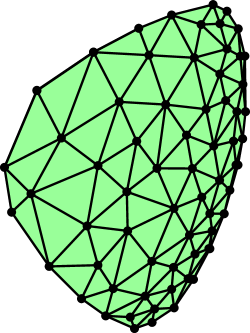
(a) with vertex selection

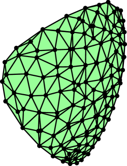
(b) without vertex selection

 

Figure 3: Inner approximations of the upper image for Example 5.1 with $a=7$; with vertex selection LABEL:sub@fig:ex1vs and without LABEL:sub@fig:ex1wo. Each vertex corresponds to a weak minimizer. One can see that without vertex selection there are many vertices in close proximity to each other, especially in regions that exhibit a large curvature (bottom right). With vertex selection, the vertices are “spread more evenly” across the surface.

Table 2: Number of quadratic problems solved with and without using the equivalence in Corollary 4.4 for different values of $a$ and $\varepsilon=0.05$ in Example 5.1.

$a$	Cor. 4.4 ✓ ✗
5	417 3348
7	640 4060
10	1019 4849
20	871 4420

Example 5.2 (Regularization parameter tracking in machine learning).

Regularized learning has been a common practice in machine learning over the past years. One of the heavily studied approaches is the elastic net:

$$\min\;\alpha_{1}\left\lVert{Ax-b}\right\rVert^{2}+\alpha_{2}\left\lVert{x}\right\rVert_{1}+\alpha_{3}\left\lVert{x}\right\rVert^{2},$$ (16)

where $A$ and $b$ are a matrix and a vector of appropriate sizes containing observed data and $\left\lVert{\cdot}\right\rVert_{1}$ denotes the $\ell_{1}$-norm. The weight vector $\alpha=(\alpha_{1},\alpha_{2},\alpha_{3})^{\mathsf{T}}$ steers the influence of the loss function $\left\lVert{Ax-b}\right\rVert^{2}$ and the regularization terms $\left\lVert{x}\right\rVert_{1}$ and $\left\lVert{x}\right\rVert^{2}$ relative to each other. The task of choosing $\alpha$ is called regularization parameter tracking and is a difficult problem on its own. While there are approaches to this problem for certain classes [see 13, 9], often one has to solve Problem (16) for every $\alpha$ on a grid in the parameter domain. The authors of [14] propose a new method by observing that Problem (16) is the weighted sum scalarization of the VCP

$$\min\begin{pmatrix}\left\lVert{Ax-b}\right\rVert^{2}\\ \left\lVert{x}\right\rVert_{1}\\ \left\lVert{x}\right\rVert^{2}\end{pmatrix}\;\text{w.r.t.}\leqslant.$$ (17)

Applying Algorithm 1 to that problem yields a weak $\varepsilon$-solution $\mathcal{X}$ in which each weak minimizer corresponds to a different choice of $\alpha$. By the definition of an infimizer we have that for every $\alpha\in\mathbb{R}^{3}$ there is some $x\in\mathcal{X}$ which is $\varepsilon$-optimal for Problem (16). Therefore we obtain a selection of parameters that is optimal up to a tolerance of $\varepsilon$.

The elastic net is frequently used in microarray classification and gene selection, a problem in computational biology. A key characteristic of such problems is that the dimension of the variable space is much larger than the number of observations. As overfitting is a major concern in such a scenario, regularized approaches are favorable [cf. 45]. Due to the problem dimension, solving scalarizations becomes costly. Therefore VS may be advantageous whenever $n\gg q$. We applied the elastic net to the following data sets:

• Lung [33] with $n=$ 12,600 features and $m=203$ instances,

• arcene [20] with $n=$ 10,000 and $m=100$,

• GLI-85 [44] with $n=$ 22,283 and $m=85$,

• MLL [33] with $n=$ 12,582 and $m=72$,

• Ovarian [34] with $n=$ 15,154 and $m=253$,

• SMK-CAN-187 [44] with $n=$ 19,993 and $m=187$,

• 14-cancer [22] with $n=$ 16,063 and $m=198$.

The data sets have been scaled such that the response is centered and the predictors are standardized:

$$\sum_{i=1}^{m}b_{i}=0,\quad\sum_{i=1}^{m}A_{i,j}=0,\quad\sum_{i=1}^{m}A_{i,j}^{2}=1,$$

for $j=1,\dots,n$. We use 70% of the data for training and 30% for testing. Table 3 shows the approximation errors and the test data mean squared error (MSE) after one hour of runtime. Evidently the approximation error is smaller with vertex selection in all test cases, while the MSE is mostly unaffected by the chosen method.

Table 3: Experimental data for Example 5.2. Highlighted in green are the lower ones of the MSEs computed by the methods for every data set.

Data Set	VS	$\varepsilon$	MSE
Lung	✓ ✗	0.3017 0.8549	0.3685 0.3353
arcene	✓ ✗	0.0179 0.0296	0.1799 0.1682
GLI-85	✓ ✗	0.0251 0.0330	0.0915 0.0823
MLL	✓ ✗	0.0161 0.0340	0.0546 0.0546
Ovarian	✓ ✗	0.6380 0.7442	0.0096 0.0096
SMK-CAN-187	✓ ✗	0.4126 0.7774	0.1655 0.1659
14-cancer	✓ ✗	4.4348 11.0260	7.7194 7.7961

Example 5.3 (Planar truss design).

In this example we discuss a problem from structural mechanics with non-differentiable objective function. We consider a planar truss that consists of two fixed supports and four free nodes which are connected by ten beams as depicted in Figure 4. The beams are assumed to have the same cross sectional area, density, and Young’s modulus. Our aim is to distribute a net force $F$ among the four free nodes in such a way that the absolute displacement of each of these nodes is minimized. We set the following problem parameters:

beam length $\ell$	$9000$	mm
beam radii	25	mm
Young’s modulus	70,000	N/mm2
force $F$	150,000	N

For simplicity we assume a linear elasticity model. We have a total of eight variables, i.e. a horizontal and a vertical force in every free node, and four objectives, i.e. the maximum of the horizontal and vertical displacement of each free node. The relationship between the acting forces $p\in\mathbb{R}^{8}$ and the nodal displacements $d\in\mathbb{R}^{8}$ is given by

$$d=K^{-1}p,$$ (18)

where $K\in\mathbb{R}^{8\times 8}$ is called the structure stiffness matrix of the truss. $K$ depends on each beams length, radius, and rotation as well as the Young’s modulus. For more insight from a mechanical viewpoint we refer the reader to the vast amount of literature on the design of trusses, such as [2, 36]. For the optimization we induce bounds on the tension and compression in each beam of 170 N/mm². Altogether the problem can be posed as

$$\min\begin{pmatrix}\max\left\{\left\lvert d_{1,h}\right\rvert,\left\lvert d_{1,v}\right\rvert\right\}\\ \vdots\\ \max\left\{\left\lvert d_{4,h}\right\rvert,\left\lvert d_{4,v}\right\rvert\right\}\end{pmatrix}\;\text{w.r.t.}\;\leqslant$$

$$\;\text{s.t.}\;\left\{\begin{aligned} d&=K^{-1}p\\ d&=(d_{i,h},d_{i,v})_{i=1,\dots,4}^{\mathsf{T}}\\ e^{\mathsf{T}}p&=F\\ -170&\leqslant Td\leqslant 170\end{aligned}\right.$$

where $d_{i,h}$, $d_{i,v}\in\mathbb{R}$ denote the horizontal and vertical displacements of node $i$, respectively, $e\in\mathbb{R}^{8}$ is the vector of all ones, and $T\in\mathbb{R}^{10\times 8}$ is a matrix relating the nodal displacements to the stress in the beams. Note that the problem can also be formulated as a vector linear program. The computational results are reported in Table 4. As in the previous examples, a smaller solution set is computed with VS. In a practical sense this eases a decision makers choice, particularly because individual minimizers may be very different from each other, see Figure 4.

 

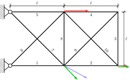
Figure 4: The planar 10-member truss from Example 5.3 with two fixed supports and four free nodes. The colored arrows illustrate different loads corresponding to weak minimizers.

Table 4: Results for Example 5.3.

$\varepsilon$	time VS ✓ VS ✗	$\lvert\mathcal{X}\rvert$ VS ✓ VS ✗
0.5	10.51 31.52	25    88
0.4	12.28 35.00	28    95
0.3	12.80 37.13	29   103
0.2	20.71 40.83	43   110

6 Conclusion

We have proposed vertex selection, a new update rule for polyhedral approximations in Benson-type algorithms for VCPs. We have shown that VS can be performed efficiently. Moreover, the approximation error is known in every iteration of the algorithm and in the provided examples fewer scalarizations need to be solved. Hence one obtains coarser solutions of VCPs with the same approximation quality while saving computation time.

References

- Batson [1986] R. G. Batson. Extensions of Radstrom’s lemma with application to stability theory of mathematical programming. J. Math. Anal. Appl. 117 (1986), pp. 441–448.
- Bendsøe and Sigmund [2003] M. P. Bendsøe and O. Sigmund. Topology design of truss structures. In Topology Optimization: Theory, Methods and Applications, Springer-Verlag, Berlin, 2003.
- Benson [1998] H. P. Benson. An outer approximation algorithm for generating all efficient extreme points in the outcome set of a multiple objective linear programming problem. J. Global Optim. 13 (1998), pp. 1–24.
- Boyd and Vandenberghe [2004] S. Boyd and L. Vandenberghe. Convex optimization. Cambridge University Press, Cambridge, 2004.
- Cheney and Goldstein [1959] E. W. Cheney and A. A. Goldstein. Newton’s method for convex programming and Tchebycheff approximation. Numer. Math. 1 (1959), pp. 253–268.
- Ciripoi et al. [2018] D. Ciripoi, A. Löhne, and B. Weißing. A vector linear programming approach for certain global optimization problems. J. Global Optim. 72 (2018), pp. 347–372.
- Csirmaz [2016] L. Csirmaz. Using multiobjective optimization to map the entropy region. Comput. Optim. Appl. 63 (2016), pp. 45–67.
- Dauer [1987] J. P. Dauer. Analysis of the objective space in multiple objective linear programming. J. Math. Anal. Appl. 126 (1987), pp. 579–593.
- Efron et al. [2004] B. Efron, T. Hastie, I. Johnstone, and R. Tibshirani. Least Angle Regression. Ann. Statist. 32 (2004), pp. 407–499.
- Ehrgott et al. [2012] M. Ehrgott, A. Löhne, and L. Shao. A dual variant of Benson’s “Outer Approximation Algorithm” for multiple objective linear programming. J. Global Optim. 52 (2012), pp. 757–778.
- Ehrgott et al. [2011] M. Ehrgott, L. Shao, and A. Schöbel. An approximation algorithm for convex multi-objective programming problems. J. Global Optim. 50 (2011), pp. 397–416.
- Ehrgott and Wiecek [2005] M. Ehrgott and M. M. Wiecek. Multiobjective programming. In Multiple Criteria Decision Analysis: State of the Art Surveys, vol. 78 of International Series in Operations Research & Management Science, J. Figueira, S. Greco, and M. Ehrgott, eds., Springer New York, 2005. pp. 667–708.
- Fischer et al. [2015] A. Fischer, G. Langensiepen, K. Luig, N. Strasdat, and T. Thies. Efficient optimization of hyper-parameters for least squares support vector regression. Optim. Methods Softw. 30 (2015), pp. 1095–1108.
- Giesen et al. [2019a] J. Giesen, S. Laue, A. Löhne, and C. Schneider. Using Benson’s algorithm for regularization parameter tracking. In The Thirty-Third AAAI Conference on Artificial Intelligence, AAAI. AAAI Press, 2019a, pp. 3689–3696.
- Giesen et al. [2019b] J. Giesen, F. Nussbaum, and C. Schneider. Efficient regularization parameter selection for latent variable graphical models via bi-level optimization. In Proceedings of the Twenty-Eighth International Joint Conference on Artificial Intelligence, IJCAI, S. Kraus, ed. ijcai.org, 2019b, pp. 2378–2384.
- Grant and Boyd [2008] M. Grant and S. Boyd. Graph implementations for nonsmooth convex programs. In Recent Advances in Learning and Control, vol. 371 of Lecture Notes in Control and Information Sciences, Springer-Verlag Limited, 2008. pp. 95–110.
- Grant and Boyd [2014] M. Grant and S. Boyd. CVX: Matlab software for disciplined convex programming, version 2.1. 2014.
- Greer [1984] R. Greer. A tutorial on polyhedral convex cones. In Trees and Hills: Methodology for Maximizing Functions of Systems of Linear Relations, vol. 96 of North-Holland Mathematics Studies, R. Greer, ed., North-Holland, 1984, chap. 2. pp. 15–81.
- Gurobi Optimization, LLC [2019] Gurobi Optimization, LLC. Gurobi Optimizer reference manual. 2019. URL http://www.gurobi.com.
- Guyon et al. [2005] I. Guyon, S. Gunn, A. Ben-Hur, and G. Dror. Result analysis of the NIPS 2003 Feature Selection Challenge. In Advances in Neural Information Processing Systems 17, MIT Press, 2005. pp. 545–552.
- Hamel et al. [2014] A. H. Hamel, A. Löhne, and B. Rudloff. Benson type algorithms for linear vector optimization and applications. J. Global Optim. 59 (2014), pp. 811–836.
- Hastie et al. [2009] T. Hastie, R. Tibshirani, and J. Friedman. The Elements of Statistical Learning: Data Mining, Inference, and Prediction. Springer Science & Business Media, 2009.
- Heyde and Löhne [2011] F. Heyde and A. Löhne. Solution concepts in vector optimization: A fresh look at an old story. Optimization 60 (2011), pp. 1421–1440.
- Jahn [1984] J. Jahn. Scalarization in vector optimization. Math. Program. 29 (1984), pp. 203–218.
- Kaibel [2011] V. Kaibel. Basic polyhedral theory. In Wiley Encyclopedia of Operations Research and Management Science, J. J. Cochran, L. A. Cox, Jr., P. Keskinocak, J. P. Kharoufeh, and J. C. Smith, eds., American Cancer Society, 2011.
- Kamenev [1992] G. K. Kamenev. A class of adaptive algorithms for the approximation of convex bodies by polyhedra. Zh. Vychisl. Mat. Mat. Fiz. 32 (1992), pp. 136–152.
- Kelley [1960] J. E. Kelley, Jr. The Cutting-plane method for solving convex programs. J. Soc. Indust. Appl. Math. 8 (1960), pp. 703–712.
- Lassez and Lassez [1992] C. Lassez and J.-L. Lassez. Quantifier elimination for conjunctions of linear constraints via a convex hull algorithm. In Symbolic and Numerical Computation for Artificial Intelligence, B. R. Donald, D. Kapur, and J. L. Mundy, eds., Academic Press, 1992.
- Luc [1987] D. T. Luc. Scalarization of vector optimization problems. J. Optim. Theory Appl. 55 (1987), pp. 85–102.
- Löhne [2011] A. Löhne. Vector Optimization with Infimum and Supremum. Springer-Verlag Berlin Heidelberg, 2011.
- Löhne et al. [2014] A. Löhne, B. Rudloff, and F. Ulus. Primal and dual approximation algorithms for convex vector optimization problems. J. Global Optim. 60 (2014), pp. 713–736.
- Löhne and Weißing [2016] A. Löhne and B. Weißing. Equivalence between polyhedral projection, multiple objective linear programming and vector linear programming. Math. Methods Oper. Res. 84 (2016), pp. 411–426.
- Mramor et al. [2007] M. Mramor, G. Leban, J. Demsar, and B. Zupan. Visualization-based cancer microarray data classification analysis. Bioinformatics 23 (2007), pp. 2147–2154.
- Petricoin et al. [2002] E. F. Petricoin, A. M. Ardekani, B. A. Hitt, P. J. Levine, V. A. Fusaro, S. M. Steinberg, G. B. Mills, C. Simone, D. A. Fishman, and E. C. Kohn. Use of proteomic patterns in serum to identify ovarian cancer. The Lancet 359 (2002), pp. 572–577.
- Rockafellar [1970] R. T. Rockafellar. Convex analysis. Princeton Mathematical Series, No. 28. Princeton University Press, Princeton, N.J., 1970.
- Rothwell [2017] A. Rothwell. Optimization Methods in Structural Design, vol. 242 of Solid Mechanics and its Applications. Springer, Cham., 2017.
- Ruzika and Wiecek [2005] S. Ruzika and M. M. Wiecek. Approximation methods in multiobjective programming. J. Optim. Theory Appl. 126 (2005), pp. 473–501.
- Shao and Ehrgott [2008a] L. Shao and M. Ehrgott. Approximately solving multiobjective linear programmes in objective space and an application in radiotherapy treatment planning. Math. Methods Oper. Res. 68 (2008a), pp. 257–276.
- Shao and Ehrgott [2008b] L. Shao and M. Ehrgott. Approximating the nondominated set of an MOLP by approximately solving its dual problem. Math. Methods Oper. Res. 68 (2008b), pp. 469–492.
- Thieu et al. [1983] T. V. Thieu, B. T. Tam, and V. T. Ban. An outer approximation method for globally minimizing a concave function over a compact convex set. Acta Math. Vietnam. 8 (1983), pp. 21–40.
- Tuy [1983] H. Tuy. On outer approximation methods for solving concave minimization problems. Acta Math. Vietnam. 8 (1983), pp. 3–34.
- Ulus [2018] F. Ulus. Tractability of convex vector optimization problems in the sense of polyhedral approximations. J. Global Optim. 72 (2018), pp. 731–742.
- Veinott [1967] A. F. Veinott, Jr. The Supporting Hyperplane Method for unimodal programming. Oper. Res. 15 (1967), pp. 147–152.
- Zhao et al. [2010] Z. Zhao, F. Morstatter, S. Sharma, S. Alelyani, A. Anand, and H. Liu. Advancing feature selection research. ASU feature selection repository (2010), pp. 1–28.
- Zou and Hastie [2005] H. Zou and T. Hastie. Regularization and variable selection via the Elastic Net. J. R. Stat. Soc. Ser. B. Stat. Methodol. 67 (2005), pp. 301–320.