Stokes parameters spectral distortions due to the Sunyaev-Zel’dovich effect and an independent estimation of the CMB low multipoles

Abstract

We consider the Stokes parameters’ frequency spectral distortions arising due to Compton scattering of the anisotropic cosmic microwave background (CMB) radiation, the Sunyaev-Zel’dovich effect (SZ), towards clusters of galaxies. We single out a very special type of such distortions and find simple analytical formulas for them. We show that this kind of distortion has a very distinctive spectral shape and can be separated from other kinds of contaminants. We demonstrate that this effect gives us an opportunity for an independent estimation of the low-multipole angular CMB anisotropies, such as the dipole, the quadrupole, and the octupole. We also show that, using distorted signals from nearby and distant clusters, one can distinguish between the Sachs-Wolfe and the integrated Sachs-Wolfe effects. The detection of such distortions can be feasible with high-angular resolution and high-sensitivity space missions, such as the upcoming Millimetron Space Observatory experiment.

I Introduction

The interaction of cosmic microwave background (CMB) radiation with hot plasma in clusters of galaxies causes the Comptonization of relic photons. This process is commonly known as the thermal Sunyaev-Zel’dovich effect (tSZ) (Zeldovich and Sunyaev, 1969a; Sunyaev and Zeldovich, 1970). As a result of this effect, a deviation in the frequency spectrum of radiation from the original CMB blackbody shape occurs. Another reason for the change in the CMB spectrum is the so-called kinematic Sunyaev-Zel’dovich effect (kSZ), which arises as a result of the peculiar cluster movements with respect to the CMB rest frame as well as the intracluster medium (ICM) motions, such as coherent gas rotations (Baldi et al., 2018) or substructure merging processes (Adam et al., 2017). Nowadays, it is clear that SZ observations with high spatial and spectral capabilities allow us to deeply exploit clusters’ ICM distribution even in the low-mass and high-redshift regimes, so complementing x-ray-band data. Correct knowledge of the thermodynamics of the cluster atmosphere is required to use them as cosmological tools and to possibly disentangle high-order-effect signals (Chluba et al., 2013; Ruppin et al., 2019) such as the ones we are interested in. The SZ effect is a very effective tool for the investigation of the internal structure of galaxies and galaxy clusters Colafrancesco and Marchegiani (2011); Colafrancesco et al. (2011); Enßlin and Kaiser (2000); Marchegiani and Colafrancesco (2015). It also has cosmological applications for the investigation of dark matter and dark energy (Colafrancesco, 2004; Weller et al., 2002), reionization (Cooray, 2006; Colafrancesco et al., 2016), and the independent estimation of the Hubble constant (Silk and White, 1978; Birkinshaw, 1979; Cavaliere et al., 1977) and CMB temperature; see Refs. (Luzzi et al., 2015; de Martino et al., 2012). In Refs. (Carlstrom et al., 2002; Mroczkowski et al., 2019), the detailed overview of the SZ effect and its use for cosmology was provided. These articles discussed the observational results, theoretical and observational challenges, various techniques, new opportunities and possible new directions in this field.

In the past thirty years, a large number of theoretical investigations connected with various corrections to the Kompaneets equation (Kompaneets, 1957) (which describes the photon spectrum evolution in electron plasma) and the SZ effect have been performed. The generalization of the Kompaneets equation, relativistic corrections to the thermal SZ effect and multiple scattering on SZ clusters were considered in Refs. (Chluba et al., 2012a; Chluba et al., 2014; Chluba and Dai, 2014; Challinor and Lasenby, 1998; Itoh et al., 1998; Stebbins, 1997; Shimon and Rephaeli, 2002; Itoh et al., 2000a; Hu et al., 1994). A detailed study of relativistic correction was made in Refs. (Nozawa et al., 1998; Sazonov and Sunyaev, 1998; Challinor and Lasenby, 1999) for kinematic SZ. In Refs. (Nozawa and Kohyama, 2009, 2013, 2014), a detailed analytical investigation of the Boltzmann equations was made for three Lorentz frames and expressions for the photon redistribution functions were derived. An effective way to separate kinematic and scattering terms was obtained in Ref. (Chluba et al., 2012b). The influence of the motion of the Solar System on the SZ signal as an additional correction was discussed in Ref. (Chluba et al., 2005).

In addition to the change in the intensity spectrum, the SZ effect also causes linear polarization, mainly due to the presence of the quadrupole component of CMB anisotropy in the galaxy cluster location (Lavaux et al., 2004; Sazonov and Sunyaev, 1999). This polarization is produced as a result of “cold” Thomson scattering in the non-relativistic regime. This effect was considered in Ref. (Kamionkowski and Loeb, 1997) for clusters at high redshifts to measure the CMB quadrupole, thereby getting around cosmic variance. In the relativistic regime other multipoles of CMB anisotropy can also contribute to the polarization of scattered radiation (Challinor et al., 2000; Shehzad Emritte et al., 2016). In addition to this, kSZ can also produce polarization (Itoh et al., 2000b). The influence of the CMB anisotropy on the spectral distortions for intensity and polarization in tSZ/kSZ was considered in Ref. (Yasini and Pierpaoli, 2016). In that work, it was shown how low multipoles form the spectrum of Stokes parameters in radiation scattered by moving clusters.

Therefore, Compton scattering of an anisotropic blackbody radiation on hot relativistic plasma creates some particular spectral features in both: radiation intensity $I$ and linear polarization parameters $Q$ and $U$. The leading term in the intensity distortion is the classical thermal SZ effect caused by the isotropic (monopole $\ell=0$) fraction of incident radiation. In addition to this, CMB anisotropy multipoles with $\ell=1,2,3$ influence the intensity of scattered radiation, causing the distortion of a very special shape (Edigaryev et al., 2018). Moreover, in the relativistic regime, polarization parameters caused by scattering will also have a very characteristic frequency of spectral features, but unlike intensity, this effect occurs due to the presence of the CMB quadrupole ($\ell=2$) and octupole ($\ell=3$).

The effects described above are in fact anisotropic corrections to the classical thermal SZ effect and follow directly from the anisotropic Kompaneets equation first derived in Ref. (Babuel-Peyrissac and Rouvillois, 1969) and generalized for polarization in Refs. (Pomraning, 1974; Stark, 1981) in linear approximation in $kT_{e}/m_{e}c^{2}$.

The amplitudes of $I,Q,U$ distortions depend on the powers of CMB $C_{1},C_{2},C_{3}$ multipoles and their orientation with respect to the axis connecting the scattering point and the observer. For the observer located at a nearby SZ cluster the CMB anisotropy map is approximately the same as we directly observe in the sky, including the quadrupole and octupole. According to Ref. (Edigaryev et al., 2018), at redshifts $z\sim 0.05$ the variations of multipole amplitudes are about $10\%$. Therefore, the measurements of intensity and polarization from such clusters allow us to estimate $\ell=1,2,3$ CMB multipoles amplitudes and their orientations. Since WMAP and Planck results show insufficient power in low-CMB anisotropy multipoles (Efstathiou, 2003; Tegmark et al., 2003; Schwarz et al., 2004; Planck Collaboration et al., 2014) and quadrupole-octupole alignment (Copi et al., 2004, 2006; Naselsky and Verkhodanov, 2008) (which is difficult to explain statistically), it is important to have an independent source of information for the estimation of $\ell=1,2,3$ multipoles. Besides, we will be able to get the information about the intrinsic dipole in our location.

The detection of such a signal from distant clusters can provide us with information about the large-angular-scale CMB anisotropy radiation coming directly from the surface of the last scattering [pure Sachs-Wolfe (SW) effect] without the influence of Rees-Sciama (RS) (Sachs and Wolfe, 1967) or integrated Sachs-Wolfe (ISW) effect.

In our paper, we derive simple analytical formulas for spectral distortions of Stokes parameters due to anisotropic tSZ effect and select the special component of these distortions which is responsible for the nonblackbody fraction of radiation (we show that all other components change the temperature, leaving the spectrum in the blackbody shape). The ratio of the amplitude of this very distinctive component to the amplitude of classical tSZ is not sensitive to the temperature or the density of the ICM and depends only on the linear combination of CMB local multipoles with $\ell=1,2,3$. We do not take into account cluster movement because our expected signal can be easily separated from the components associated with the kSZ effect. We show how to use distorted signals of this kind coming from nearby and distant clusters to estimate $\ell=1,2,3$ CMB multipoles and to distinguish between the SW and ISW effects.

It is worth mentioning that the signal we consider is very low and should be separated from other types of spectral distortions. As for intensity distortion, we have to take into account that the CMB isotropic monopole part is larger than anisotropic multipoles by a factor of $\sim 10^{5}$. This means that we should take into account relativistic corrections of higher orders to this effect. At the same time, the polarised signal is not affected by the CMB monopole. Therefore, $Q,U$ observational data will be “cleaner” than the data for intensity.

The future Millimetron mission (Wild et al., 2009; Kardashev et al., 2014; Smirnov et al., 2012) will have unprecedented sensitivity in the single-dish mode to measure the polarized signal in the range from 100 GHz to 2 THz down to sub-arcminute resolution. One of the main tasks of this mission will be the measurement of $\mu$ and $y$ spectral distortions of CMB radiation, which arise due to the energy injections into the plasma in the prerecombination epoch. These distortions can also be formed as a result of the interaction of CMB with matter during the process of large-scale structure formation (Zeldovich and Sunyaev, 1969b; Sunyaev and Zeldovich, 1970; Illarionov and Siuniaev, 1974; Burigana et al., 1991; Hu and Silk, 1993; Chluba and Sunyaev, 2012; Chluba, 2015; Chluba et al., 2019a, b; Desjacques et al., 2015; Chluba, 2014). As an additional task, the possibility of detecting the spectral distortions from SZ clusters caused by CMB anisotropy can be considered. We discuss the feasibility of this task by Millimetron in Sec. IV (Conclusions).

The outline of this paper is as follows: In Sec. II, we review the equation for the polarized radiative transfer in plasma in the relativistic regime. Using this equation, we derive analytical formulas for $I,Q,U$ distortions for scattered radiation and find expressions for observed linear combinations of multipole amplitudes. In Sec. III, we show how to estimate low CMB multipoles and how to distinguish between SW and ISW effects combining the signals from nearby and distant clusters. Finally, in Sec. IV, we make our brief conclusions.

II Stokes parameters spectral distortions due to anisotropic thermal SZ effect

In this section we review the radiative polarization transfer equations in hot Comptonizing electron plasma, which was first derived by Stark in Ref. (Stark, 1981), and we apply this approach to the consideration of CMB scattering on Sunyaev-Zel’dovich clusters. Combining results found in Refs. (Babuel-Peyrissac and Rouvillois, 1969) and (Stark, 1981) and assuming that the incident radiation is unpolarized, we find the simple analytical formulas for Stokes parameters spectral distortions that arise due to the scattering of anisotropic radiation on hot electrons.

We use the following notations:

$I(\nu,\mathbb{\Omega}),Q(\nu,\mathbb{\Omega}),U(\nu,\mathbb{\Omega})$: Stokes parameters, where $I$ is the spectral radiance, $Q$ and $U$ describe the linear polarization, $\nu$ is the frequency and $\mathbb{\Omega}$ is the radiation propagation direction.

$n=\frac{c^{2}I}{2h\nu^{3}}$: Photon concentration in phase space, where $c$ is the speed of light and $h$ is the Planck constant. We also use the notations $q=\frac{c^{2}Q}{2h\nu^{3}}$ and $u=\frac{c^{2}U}{2h\nu^{3}}$.

${\bf J}=\begin{pmatrix}n(\nu,\mathbb{\Omega})\\ q(\nu,\mathbb{\Omega})\\ u(\nu,\mathbb{\Omega})\end{pmatrix}$ is the vector that describes Stokes parameters.

$T_{e},T_{r}$: Temperatures of electrons and radiation.

$m_{e}$: Electron mass at rest.

$\Theta_{e}=\frac{kT_{e}}{m_{e}c^{2}}$, $\varepsilon=\frac{h\nu}{m_{e}c^{2}}$, $x=\frac{h\nu}{kT_{r}}$, where $k$ is the Boltzmann constant.

Figure 1: Schematic representation of radiation scattering on a SZ cluster. The scattering point (SZ cluster) is at the center of the coordinate system. This system is chosen so that the z axis is directed from the observer to the cluster. The scattered radiation is propagating to the observer in the direction opposite to the z axis. Therefore, $\Theta$ is the angle of scattering, and $\varphi$ denotes the scattering plane orientation.

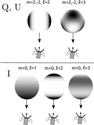
Figure 2: Schematic representation of CMB multipoles $Y_{\ell}^{m}$ in the surroundings of the cluster location that contribute to the spectral distortions of type 2. Here the z axis points from the observer to the cluster in the corresponding spherical coordinate system. Upper panel: $Q,U$ are affected by $\ell=2,3$ and $m=\pm 2$. Lower panel: Intensity $I$ is distorted by axisymmetric multipoles $\ell=1,2,3$, $m=0$.

The equation for the radiative transfer in plasma for anisotropic radiation was first derived in Ref. (Babuel-Peyrissac and Rouvillois, 1969) and generalized for the polarized radiation in Ref. (Stark, 1981). It can be used for relatively cold photons and electrons: $kT_{e}\ll m_{e}c^{2}$, $h\nu\ll m_{e}c^{2}$. This approximation works pretty well for SZ clusters with $T_{e}\sim 10$ keV and CMB temperature $T_{r}\sim 3$ K. This approach implies the correction to the Thomson scattering up to the first order in $\varepsilon$, $\Theta_{e}$. In our investigation, we assume an optically thin limit, so that photons propagating through the cluster can scatter only once, and the radiation before scattering is unpolarized and anisotropic. Thus, if we denote the Stokes parameters by “prime” values $n^{{}_{{}^{\prime}}},q^{{}_{{}^{\prime}}},u^{{}_{{}^{\prime}}}$ before scattering, then $q^{{}_{{}^{\prime}}}=u^{{}_{{}^{\prime}}}=0$. In order to separate the isotropic and anisotropic parts of radiation, it is convenient to use $\bar{n}(\nu)=\frac{1}{4\pi}\int n^{{}_{{}^{\prime}}}(\nu,\mathbb{\Omega})d\mathbb{\Omega}$ and $\Delta=n^{{}_{{}^{\prime}}}(\nu,\mathbb{\Omega})-\bar{n}(\nu)$.

Using our notations and omitting some obvious algebra in the case of single scattering, we can rewrite the polarization transfer equation in hot Comptonizing electron plasma found in Ref. (Stark, 1981) as follows:

$$\begin{array}[]{l}\vspace{0.2cm}\delta{\bf J}/\delta\tau=\frac{3}{16\pi}\bigint\limits_{\mathbb{\Omega}}\Big{\{}\left.\Delta{\bf R}+\Theta_{e}\Delta\left({\bf S}-2\frac{T_{r}}{T_{e}}{\bf R}\right)\right.+\\ \vspace{0.5cm}\left.\Theta_{e}G_{a}(\Delta)(1-\mu){\bf R}\right.\Big{\}}d\mathbb{\Omega}+\Theta_{e}G_{i}(\bar{n}){\bf T}+O(\Theta^{2}),\\ \vspace{0.5cm}\par{\bf R}=\begin{pmatrix}1+\mu^{2}\\ (1-\mu^{2})\cos 2\varphi\\ (1-\mu^{2})\sin 2\varphi\end{pmatrix},\hskip 14.22636pt{\bf T}=\begin{pmatrix}1\\ 0\\ 0\end{pmatrix}\\ \vspace{0.5cm}\par{\bf S}=2\begin{pmatrix}(1-\mu)^{2}(1+2\mu)-4\mu\\ (1-\mu^{2})(1+2\mu)\cos 2\varphi\\ (1-\mu^{2})(1+2\mu)\sin 2\varphi\end{pmatrix},\hskip 5.69046ptd\mathbb{\Omega}=d\mu d\varphi\\ \vspace{0.5cm}\par G_{a}(\Delta)=\frac{1}{x^{2}}\frac{\partial}{\partial x}\left[x^{4}\left(\frac{T_{r}}{T_{e}}\Delta+\frac{\partial\Delta}{\partial x}\right)\right]+2\frac{T_{r}}{T_{e}}n^{{}_{{}^{\prime}}}\frac{\partial}{\partial x}\left[x^{2}\Delta\right],\\ \vspace{0.5cm}\par G_{i}(\bar{n})=\frac{1}{x^{2}}\frac{\partial}{\partial x}\left[x^{4}\left(\frac{T_{r}}{T_{e}}(\bar{n}+\bar{n}^{2})+\frac{\partial\bar{n}}{\partial x}\right)\right].\par\end{array}$$ (1)

Here $\delta\tau$ is the optical depth, and $\mu=\cos\Theta$ is the cosine of the scattering angle. The azimuthal angle $\varphi$ shows the orientation of the scattering plane (Fig 1). Functions $G_{a}$ and $G_{i}$ represent the anisotropic and isotropic parts of radiation, respectively. Since the radiation temperature is much less than the temperature of plasma in galaxy clusters one can neglect all the terms proportional to $T_{r}/T_{e}$ in Eq. (1):

$$\begin{array}[]{l}\vspace{0.2cm}\delta{\bf J}/\delta\tau=\\ \vspace{0.5cm}\par\frac{3}{16\pi}\bigint\limits_{\mathbb{\Omega}}\Big{\{}\Delta\left({\bf R}+\Theta_{e}{\bf S}\right)+G(\Delta)\Theta_{e}(1-\mu){\bf R}\Big{\}}d\mathbb{\Omega}\\ \vspace{0.5cm}\par+\Theta_{e}G(\bar{n}){\bf T}+O(\Theta^{2}),\hskip 14.22636ptG(f)=\frac{1}{x^{2}}\frac{\partial}{\partial x}\left[x^{4}\frac{\partial f}{\partial x}\right],\end{array}$$ (2)

with $f$ equal to $\Delta$ or $\bar{n}$. The CMB radiation frequency spectrum can be considered as a blackbody spectrum with high accuracy (Fixsen, 2009) . Therefore, the shape of the spectrum can be completely described by the radiation temperature $T_{r}$. Since the relic radiation is anisotropic, its temperature varies with direction. Thus, for the radiation incident on a cluster we can write the following formulas:

$$\begin{array}[]{l}\vspace{0.5cm}\par n^{{}_{{}^{\prime}}}(x,\mathbb{\Omega})=B(x)-x\frac{dB}{dx}\hskip 2.84544pt\frac{\Delta_{T}(\mathbb{\Omega})}{T_{r}},\hskip 14.22636ptB(x)=\frac{1}{e^{x}-1},\\ \vspace{0.5cm}\par\Delta_{T}(\mathbb{\Omega})=T(\mathbb{\Omega})-T_{r},\\ \vspace{0.5cm}\par\bar{n}(x)=B(x),\hskip 28.45274pt\Delta=-x\frac{dB}{dx}\hskip 2.84544pt\frac{\Delta_{T}(\mathbb{\Omega})}{T_{r}}.\par\par\end{array}$$ (3)

Substituting these formulas into Eq. (2), we get very simple analytical results for Stokes parameters spectral distortions after a single scattering:

$$\begin{array}[]{l}\vspace{0.2cm}\delta{\bf J}/\delta\tau=\\ \vspace{0.5cm}\par g_{1}(x)\left[\frac{3}{16\pi}\int\limits_{\mathbb{\Omega}}\frac{\Delta_{T}(\mathbb{\Omega})}{T_{r}}\left({\bf R}+\Theta_{e}{\bf S}\right)d\mathbb{\Omega}\right]+\hskip 11.38092pt\Big{\}}1\\ \vspace{0.5cm}\par+\Theta_{e}g_{2}(x)\left[\frac{3}{16\pi}\int\limits_{\mathbb{\Omega}}\frac{\Delta_{T}(\mathbb{\Omega})}{T_{r}}(1-\mu){\bf R}d\mathbb{\Omega}\right]+\hskip 5.69046pt\Big{\}}2\\ \vspace{0.5cm}\par+\Theta_{e}g_{3}(x){\bf T},\hskip 85.35826pt\Big{\}}3\hskip 5.69046pt(tSZ)\\ \vspace{0.5cm}\par g_{1}(x)=-x\frac{dB}{dx},\hskip 14.22636ptg_{2}(x)=\frac{1}{x^{2}}\frac{d}{dx}\left[x^{4}\frac{d}{dx}\left(-x\frac{dB}{dx}\right)\right],\\ \vspace{0.5cm}\par g_{3}(x)=\frac{1}{x^{2}}\frac{d}{dx}\left[x^{4}\frac{dB}{dx}\right]\end{array}$$ (4)

The expression for $\delta J/\delta\tau$ consists of three terms. They represent spectral distortions of three different types $g_{1}$, $g_{2}$, and $g_{3}$. Below, we describe the physical meaning of these three terms and analyze the possibility to use them for the investigation of CMB properties.

1. The first term represents Thompson scattering with some correction proportional to $\Theta_{e}$. This term arises due to mixing flows with different temperatures in the process of scattering and represents distortion of the form $g_{1}=-x\frac{dB}{dx}$. It is rather difficult to use distortion of this kind in real observations for the following reasons:
a. The first Stokes parameter $I$ (or $n$) after scattering preserves its spectral shape in the form of a blackbody but with a bit different temperature. Indeed, in the linear approximation the term $-x\frac{dB}{dx}\frac{\Delta_{T}}{T_{r}}$ is in fact the difference between two blackbody spectra with temperatures $T_{r}$ and $T_{r}+\Delta T$. Thus the amplitude of such deviation depends on the value of the mean temperature $T_{r}$.
b. The CMB is slightly polarized and its linear polarization parameters have a spectral shape in the form of $g_{1}$. Therefore, Stokes parameters $q$ and $u$ of the radiation propagating through the cluster to the observer without scattering have the same spectral shape as the Stokes parameters for the scattered fraction of radiation. Thus, scattered and unscattered fractions can be confused with each other if we use this type of polarization spectral distortion.

2. The second term represents distortion of the form $g_{2}(x)=\frac{1}{x^{2}}\frac{d}{dx}\left[x^{4}\frac{d}{dx}\left(-x\frac{dB}{dx}\right)\right]$. This effect occurs due to Comptonization of anisotropic incident radiation on hot electrons. Such distortion has a very characteristic and distinctive nonblackbody shape for all three Stokes parameters. Using distortions of this type gives us a unique opportunity to separate the scattered fraction of radiation from the unscattered one. In our previous paper (Edigaryev et al., 2018), we analyzed this distortion only for the first Stokes parameter $n$, calling this effect an “anisotropic thermal SZ effect.”

3. The third term is the classical thermal SZ effect: $g_{3}(x)=\frac{1}{x^{2}}\frac{d}{dx}\left[x^{4}\frac{dB}{dx}\right]$. This term represents the distortion for the isotropic part of incident radiation. It affects the $n$ parameter only, without modifying linear polarization:

$$\delta\mathbb{J_{3}}=\begin{pmatrix}\delta n_{{}_{3}}\\ \delta q_{{}_{3}}\\ \delta u_{{}_{3}}\end{pmatrix}=g_{3}(x)\begin{pmatrix}1\\ 0\\ 0\end{pmatrix}\Theta_{e}\delta\tau,$$ (5)

where the index 3 means that we take into account distortion of the form $g_{3}$.

Let us consider how low multipoles of CMB anisotropy contribute to the Stokes parameters spectral distortions of the form $g_{2}(x)$. This is the distortion which is of particular interest to us and the only type of distortion we will analyze below. We will denote this part of the distortion by the index 2.

The temperature fluctuations of radiation incident to the SZ cluster can be described in terms of spherical harmonics $Y_{\ell}^{m}(\mathbb{\Omega})$:

$$\frac{\Delta_{T}(\mathbb{\Omega})}{T_{r}}=\sum\limits_{\ell=1}^{\infty}\sum\limits_{m=-\ell}^{\ell}\tilde{a}_{\ell,m}Y_{\ell}^{m}(\mathbb{\Omega}),$$ (6)

where $\tilde{a}_{\ell,m}$ are the coefficients for $\Delta_{T}/T_{r}$ decomposition for a given location of the galaxy cluster ($\tilde{a}_{\ell,m}$ are not the same as $a_{\ell,m}$ for the conventional Galactic coordinate system). We choose a local spherical coordinate system at the scattering point in such a way that the south pole corresponds to the direction from the SZ cluster to the observer (see Fig. 1). Substituting Eq. (6) into the second term of Eq. (4), we get

$$\begin{array}[]{l}\vspace{0.3cm}\par\frac{\delta n_{{}_{2}}}{\delta\tau}=-\frac{3}{4\sqrt{\pi}}\left(\frac{4}{5\sqrt{3}}\tilde{a}_{1,0}-\frac{1}{3\sqrt{5}}\tilde{a}_{2,0}+\frac{1}{5\sqrt{7}}\tilde{a}_{3,0}\right)\Theta_{e}g_{2}(x),\\ \vspace{0.3cm}\par\frac{\delta q_{{}_{2}}}{\delta\tau}=\frac{3}{4\sqrt{5\pi}}\left(\tilde{a}_{2,2}-\frac{1}{\sqrt{7}}\tilde{a}_{3,2}\right)\Theta_{e}g_{2}(x),\\ \vspace{0.3cm}\par\frac{\delta u_{{}_{2}}}{\delta\tau}=\frac{3}{4\sqrt{5\pi}}\left(\tilde{a}_{2,-2}-\frac{1}{\sqrt{7}}\tilde{a}_{3,-2}\right)\Theta_{e}g_{2}(x).\par\end{array}$$ (7)

Therefore, only multipoles with $\ell=1,2,3$ contribute to this kind of distortion. In Fig. 2, you can see the schematic demonstration of the local CMB anisotropy multipoles that contribute to the distortion of the observed Stokes parameters. The first parameter $n$ is distorted by axisymmetric local multipoles $Y_{\ell}^{0}$, $\ell=1,2,3$, while the linear polarization parameters $q$ and $u$ are distorted due to the presence of multipoles with $m=\pm 2$: $Y_{2}^{\pm 2}$ and $Y_{3}^{\pm 2}$. It is worth noticing, that the orientation of the distorted part of linear polarization is different from the orientation of polarization caused by pure “cold” Thomson scattering. It happens because Thomson scattering produces linear polarization due to the presence of harmonics $\ell=2$, $m=\pm 2$ in the anisotropy, while the distorted part of the polarization is produced by harmonics with $\ell=2,3$,  $m=\pm 2$. We can write the following formulas:

$$\begin{array}[]{l}\vspace{0.2cm}\par\tan(2\psi_{2})=\frac{u_{2}}{q_{2}}=\frac{\tilde{a}_{2,-2}-\frac{1}{\sqrt{7}}\tilde{a}_{3,-2}}{\tilde{a}_{2,2}-\frac{1}{\sqrt{7}}\tilde{a}_{3,2}},\\ \vspace{0.2cm}\par\tan(2\psi_{cold})=\frac{u_{cold}}{q_{cold}}=\frac{\tilde{a}_{2,-2}}{\tilde{a}_{2,2}},\end{array}$$

where $\psi_{2}$ and $\psi_{cold}$ are the distorted polarization orientation and the orientation of the polarization caused by Thomson scattering respectively. We can always rotate the coordinate system in such a way that $\hat{u}_{cold}=0$ and $\psi_{cold}=0$. Therefore, we can estimate the angle between the orientations of the Thomson polarization and the distorted part of the linear polarization in terms of coefficients $\hat{a}_{ell,m}$ in the rotated (“hat”) coordinate system:

$$\begin{array}[]{l}\psi_{2}-\psi_{cold}=-\frac{1}{2}\arctan\left(\frac{\hat{a}_{3,-2}}{\sqrt{7}\hat{a}_{2,2}-\hat{a}_{3,2}}\right).\\ \end{array}$$

In order to estimate the CMB anisotropy multipoles at the SZ cluster location we should divide the amplitude of the observed distorted signal proportional to $g_{2}$ by the amplitude of the classical thermal SZ effect, which is proportional to $g_{3}$ [Eq. 5]. In this case, we can get rid of the Comptonization parameter $\Theta_{e}\delta_{\tau}$ and find the following coefficients $\beta$:

$$\begin{array}[]{l}\vspace{0.3cm}\par\beta_{n}=-\frac{3}{4\sqrt{\pi}}\left(\frac{4}{5\sqrt{3}}\tilde{a}_{1,0}-\frac{1}{3\sqrt{5}}\tilde{a}_{2,0}+\frac{1}{5\sqrt{7}}\tilde{a}_{3,0}\right),\\ \vspace{0.3cm}\par\beta_{q}=\frac{3}{4\sqrt{5\pi}}\left(\tilde{a}_{2,2}-\frac{1}{\sqrt{7}}\tilde{a}_{3,2}\right),\\ \vspace{0.3cm}\par\beta_{u}=\frac{3}{4\sqrt{5\pi}}\left(\tilde{a}_{2,-2}-\frac{1}{\sqrt{7}}\tilde{a}_{3,-2}\right).\par\end{array}$$ (8)

Therefore, by observing distorted radiation coming from a SZ cluster one can find three coefficients $\beta_{n}$, $\beta_{q}$ and $\beta_{u}$ that are the linear combinations of the local harmonics amplitudes with $\ell=1,2,3$ and $-\ell\leq m\leq\ell$.

We should mention that the intensity spectral distortions are affected by the isotropic part of CMB radiation, which is 5 orders of magnitude larger than the anisotropic one. At the same time, the linear polarization induced by the SZ effect arises due to the anisotropic fraction only. This means that in the process of component separation for intensity, we should take into account relativistic corrections to tSZ of higher orders (Challinor and Lasenby, 1998). In addition to this, relativistic corrections due to bulk motion of hot clusters should be also taken into account (Sazonov and Sunyaev, 1998). Thermal corrections are proportional to $\tau\Theta_{e}^{k}$, $k>1$ (see Fig 3). The observational data for polarization will be free of such corrections, and therefore will be “cleaner” than the intensity data.

It is worth noticing, that the anisotropy in the cluster medium together with the multiple scattering can induce an additional local radiation anisotropy. When CMB scatters on a cluster’s medium, the radiation frequency spectrum becomes distorted mainly due to the tSZ effect. As a result of this effect, radiation incident to the point of the last scattering before propagating to the observer receives an additional anisotropy. This induced anisotropy $\Delta_{in}$ is the anisotropy of the tSZ amplitude (not the temperature anisotropy of a blackbody radiation). Such an anisotropy arises due to different medium temperatures $\Theta_{e}(\mathbb{\Omega})$ and optical depths $\delta_{\tau}(\mathbb{\Omega})$ in different directions $\mathbb{\Omega}$ from the point of the last scattering:

$$\Delta_{in}(x,\mathbb{\Omega})=\frac{1}{x^{2}}\frac{d}{dx}\left[x^{4}\frac{dB}{dx}\right]\Theta_{e}(\mathbb{\Omega})\delta_{\tau}(\mathbb{\Omega})$$

[compare with $\Delta$ in Eq. (3)]. Therefore, this kind of anisotropy will create an additional spectral distortion, but the shape of such a distortion will be different from what we are considering.

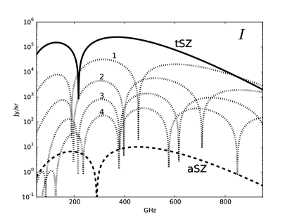
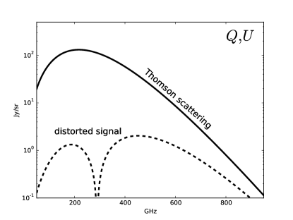
Figure 3: A distorted signal of type 2 for the intensity and polarization from a cluster with optical depth $\tau=0.01$ and temperature $T_{e}=7$ keV. Upper panel: The solid line shows the classical tSZ effect, dotted lines show relativistic corrections to tSZ up to the fourth order, and the dashed line corresponds to the type 2 intensity distortion [“anisotropic SZ effect” (aSZ)]. Note that the aSZ crosses zero at a different frequency respecting the tSZ zero-crossing point. The amplitude and the sign of the aSZ effect depend on $\Theta_{e}\delta\tau$ and the linear combination of $a_{\ell m}$ [see Eq 7]. Lower panel: The solid line shows the spectrum for the linear polarization caused by “cold” Thomson scattering, and the dashed line is the spectrum of the type 2 distortion of the polarized fraction.

In the next section, we show how to use Eq. (8) for the independent estimation of low CMB multipoles using nearby clusters. We will also demonstrate how to distinguish between the SW and ISW effects combining the signals from nearby and distant clusters.

III The independent estimation of low-CMB anisotropy multipoles and possibile separation of SW and ISW effects

In this section, we describe the method to reconstruct the CMB dipole, quadrupole, and octupole at our location and show how to separate contributions from the SW and ISW effects on CMB anisotropy by observing the distorted signals from SZ galaxy clusters.

As it follows from Eq. (8), the spectral distortion intensity depends on the linear combination of components of $\ell=1,2,3$ spherical harmonics, while the polarized signal depends on components with $\ell=2,3$. For both polarized and unpolarized signals, the components which contribute to the signal are projected on the axis pointing from the observer to the cluster. If the coefficients of spherical harmonics, $a_{\ell,m}$, were the same over the Universe, then by observing different clusters, it would be possible to measure different projections of these spherical harmonics, and thus reconstruct the full set of coefficients for $\ell=1,2,3$.

In reality, $a_{\ell,m}$ are not the same over the space, because low-$\ell$ harmonics are significantly affected by the ISW effect. According to Ref. Crittenden and Turok (1996), about 40% of the quadrupole amplitude and 25% of the octupole amplitude are generated by the ISW effect. In our previous paper (Edigaryev et al., 2018) we analyzed the spatial correlations of $a_{\ell,m}$ and concluded that at distances less than 250 $h^{-1}$ Mpc from the Earth, the coefficients may differ no more than 10% from the $a_{\ell,m}$ which we would observe in the absence of foregrounds. This will allow us to reconstruct local $a_{\ell,m}$ by observing $\sim$170 nearby clusters at $z<0.085$ (which corresponds to 250 $h^{-1}$ Mpc).

In Figs. 4 and 5, we show the maps of the expected intensity and polarization distortions of type 2 for the scattered radiation coming from nearby SZ clusters located at particular positions in the sky. These maps correspond to the values of $a_{\ell,m}$ for $\ell=2,3$ measured by Planck (Planck Collaboration et al., 2018). In the case of intensity, we did not take into account the intrinsic CMB dipole, since it is completely overshadowed by our motion with respect to the CMB rest frame. In Fig. 4, we show the celestial map in Galactic coordinates, where the value of the intensity distortion is indicated by the shade of gray, and lines correspond to the orientation and amplitude of polarization, determined by $\beta_{q}$ and $\beta_{u}$. In Fig. 5, we show the amplitude of the distorted polarized signal, i.e., $\sqrt{\beta_{q}^{2}+\beta_{u}^{2}}$. A lighter color corresponds to stronger polarization.

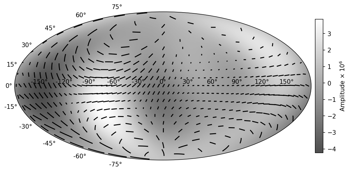
Figure 4: Map of the unpolarized signal amplitude, shown with gray color. The polarized signal determined by $\beta_{q}$ and $\beta_{u}$ is shown by short lines. The map is based on values of $a_{\ell,m}$ given by the Planck Collaboration (Planck Collaboration et al., 2018).

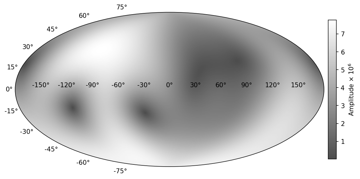
Figure 5: Map of polarization amplitude, $\sqrt{\beta_{q}^{2}+\beta_{u}^{2}}$, based on values of $a_{\ell,m}$ given by the Planck Collaboration (Planck Collaboration et al., 2018). Lighter colors correspond to stronger polarization.

If we look at distances $\geq$ $1000\,h^{-1}$ Mpc, the ISW effect is weak, and low-$\ell$ anisotropy of CMB is created by the SW effect on the last scattering surface. The coefficients $a_{\ell,m}$ weakly depend on the redshift, if we consider clusters at distances 1000$\,h^{-1}$ Mpc $<R<$ 2000$\,h^{-1}$ Mpc. Reconstruction of $a_{\ell,m}$ at these distances will allow us to measure the low-$\ell$ CMB anisotropy at the last scattering surface, i.e., without the ISW effect.

Now we will show how the reconstruction of $a_{\ell,m}$ from measurements of $\beta_{n}$, $\beta_{q}$ and $\beta_{u}$ for a set of clusters can be done, and how measurements of polarization can improve the precision of reconstruction. We imply that $a_{\ell,m}$ are the same for the window of distances we consider. The signal in Eq. (8) depends on the values of $\tilde{a}_{1,0}$, $\tilde{a}_{2,0}$, $\tilde{a}_{3,0}$, $\tilde{a}_{2,\pm 2}$, $\tilde{a}_{3,\pm 2}$, where the tilde denotes that the coefficients are given in a rotated coordinate system. The rotation needed to obtain $\tilde{a}_{\ell,m}$ from $a_{\ell,m}$ is defined as follows: For a cluster with Galactic sky coordinates $l,b$ we first rotate the system around z axis by $-l$, and then rotate about the new y axis by $90-b$ degrees. For any cluster location, we can express the three signals ($\beta_{n}$, $\beta_{q}$, $\beta_{u}$) as a linear combination of all 15 $a_{\ell,m}$’s with $\ell=1,2,3$. The coefficients in this linear combination depend on the celestial coordinates. As a result, for $N$ different celestial locations we have a set of $3N$ linear equations. The values of $a_{\ell,m}$ can be determined by fitting a linear model to the measured signals.

We can estimate the relative precision of $a_{\ell,m}$ determination for known SZ clusters from the PLANCKSZ2 catalog (Planck Collaboration et al., 2016) by using the maximum likelihood estimator. We start with 15 clusters at $R>1000$ $h^{-1}$ Mpc, as this is the minimum number of clusters needed to find $a_{\ell,m}$ in the case where we measure only the unpolarized signal, $\beta_{n}$. We set the error of $a_{\ell,m}$ determination to 1.0 for this sample of 15 clusters and the case when only $\beta_{n}$ is used. We grow the sample by adding more clusters at larger distances, and we consider either using only the unpolarized signal, or the full signal. The results are shown in Fig. 6. As one can see from this figure, the precision of octupole and quadrupole determination is improved by a factor of 3, when the polarization measurements are used.

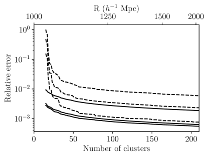
Figure 6: Relative error of determination of amplitudes of dipole, quadrupole and octupole (from bottom to top) with respect to an error for a minimal sample of 15 clusters, as a function of the cumulative number of clusters in a sample growing from 1000$\,h^{-1}$ to 2000$\,h^{-1}$ Mpc. Solid lines correspond to the usage of the full (polarized + unpolarized) signal; dashed lines correspond to only the unpolarized signal ($\beta_{n}$).

Observing two samples of clusters, one at $R<250\,h^{-1}$ Mpc and another one at $R>1000$ $h^{-1}$ Mpc, will allow us to distinguish between SW and ISW effects. Using the first sample, we will determine local $a_{\ell,m}$ created by both SW and ISW effects, but free from the contamination by zodiacal light and our Galaxy’s dust. By measuring the signal from distant clusters in the second sample, we will reconstruct the $a_{\ell,m}$ created only by the SW effect. The relative precision for $a_{\ell,m}$ reconstruction will remain the same as in our previous paper (Edigaryev et al., 2018) if we only use the intensity distortions. We would remind the reader that the reconstruction of coefficients with $m=\ell$ is more complicated. This is mainly because most of the power of such harmonics is close to the Galactic plane, where the number of clusters observed by Planck is limited.

IV Conclusions

In our paper, we considered polarized thermal SZ effect and derived an analytical result for a very distinctive component of spectral distortions in Stokes parameters which arise due to the presence of dipole, quadrupole, and octupole CMB angular anisotropy. We showed that this type of distortion can be disentangled from other components and can be used for the independent estimation of $\ell=1,2,3$ CMB multipole amplitudes and their orientation. We demonstrated that by observing distorted radiation from nearby clusters it is possible to estimate independently CMB anisotropy coefficients $a_{\ell,m}$, $\ell=1,2,3$, $-\ell\leq m\leq\ell$ in our location. We also proposed a method for the separation of ISW and SW effects by combining observations of distorted signals from distant and nearby clusters.

In this work, we did not discuss foreground component separation or the impact of kSZ, relativistic corrections, and CMB photon multiple scattering. The peculiar spectral shape of the type of distortions considered here allows us to disentangle them from other contaminants. The anisotropies in the cluster medium together with the double scattering can induce additional local anisotropy which should also be taken into account. The large number of clusters in the same redshift range and same sky direction will provide us with good statistics, which can help to solve this problem. Besides this, Millimetron, with its unprecedented combination of high angular resolution and high sensitivity in a wide spectral range will allow us to deeply observe individual clusters, providing accurate maps of the ICM pressure distribution. We stress that under the assumption of a single scattering approximation, the ratio of the anisotropic SZ effect and the thermal one, aSZ/tSZ, is independent of the gas temperature and optical depth.

The signal we considered is strong enough for its detection with the Millimetron mission to be feasible in principle. Nevertheless, with today’s technologies, it implies a very long integration time. We should mention also that accurate knowledge of the instrumental polarization purity (cross polarization and/or instrumental induced polarization) is mandatory to avoid possible leakages between observed Stokes parameters, which can create irremovable systematic errors. It can affect our capability to detect such a tiny spectral distortion in linear polarization.

V Acknowledgments

We wish to thank the referee for very useful discussion. The work is supported by the Project No. 01-2018 of LPI new scientific groups and the Foundation for the Advancement of Theoretical Physics and Mathematics “BASIS”, Grant No. 19-1-1-46-1. M.D.P. acknowledges support from Sapienza Università di Roma thanks to Progetti di Ricerca Medi 2019, No. RM11916B7540DD8D.

References

- Zeldovich and Sunyaev (1969a) Y. B. Zeldovich and R. A. Sunyaev, Astrophys. Space. Sci 4, 301 (1969a).
- Sunyaev and Zeldovich (1970) R. A. Sunyaev and Y. B. Zeldovich, Astrophys. Space. Sci 7, 20 (1970).
- Baldi et al. (2018) A. S. Baldi, M. De Petris, F. Sembolini, G. Yepes, W. Cui, and L. Lamagna, Mon. Not. R. Astron. Soc 479, 4028 (2018), eprint 1805.07142.
- Adam et al. (2017) R. Adam, I. Bartalucci, G. W. Pratt, P. Ade, P. André, M. Arnaud, A. Beelen, A. Benoît, A. Bideaud, N. Billot, et al., Astron. Astrophys 598, A115 (2017), eprint 1606.07721.
- Chluba et al. (2013) J. Chluba, E. Switzer, K. Nelson, and D. Nagai, Mon. Not. R. Astron. Soc 430, 3054 (2013), eprint 1211.3206.
- Ruppin et al. (2019) F. Ruppin, F. Mayet, J. F. Macías-Pérez, and L. Perotto, Mon. Not. R. Astron. Soc 490, 784 (2019), eprint 1905.05129.
- Colafrancesco and Marchegiani (2011) S. Colafrancesco and P. Marchegiani, Astron. Astrophys 535, A108 (2011), eprint 1108.4602.
- Colafrancesco et al. (2011) S. Colafrancesco, P. Marchegiani, and R. Buonanno, Astron. Astrophys 527, L1 (2011).
- Enßlin and Kaiser (2000) T. A. Enßlin and C. R. Kaiser, Astron. Astrophys 360, 417 (2000), eprint astro-ph/0001429.
- Marchegiani and Colafrancesco (2015) P. Marchegiani and S. Colafrancesco, Mon. Not. R. Astron. Soc 452, 1328 (2015), eprint 1506.05651.
- Colafrancesco (2004) S. Colafrancesco, Astron. Astrophys 422, L23 (2004), eprint astro-ph/0405456.
- Weller et al. (2002) J. Weller, R. A. Battye, and R. Kneissl, Phys. Rev. Lett. 88, 231301 (2002), eprint astro-ph/0110353.
- Cooray (2006) A. Cooray, Phys. Rev. D 73, 103001 (2006), eprint astro-ph/0511240.
- Colafrancesco et al. (2016) S. Colafrancesco, P. Marchegiani, and M. S. Emritte, Astron. Astrophys 595, A21 (2016), eprint 1607.07723.
- Silk and White (1978) J. Silk and S. D. M. White, Astrophys. J., Lett 226, L103 (1978).
- Birkinshaw (1979) M. Birkinshaw, Mon. Not. R. Astron. Soc 187, 847 (1979).
- Cavaliere et al. (1977) A. Cavaliere, L. Danese, and G. de Zotti, Astrophys. J 217, 6 (1977).
- Luzzi et al. (2015) G. Luzzi, R. T. Génova-Santos, C. J. A. P. Martins, M. De Petris, and L. Lamagna, Journal of Cosmology and Astroparticle Physics 2015, 011 (2015), eprint 1502.07858.
- de Martino et al. (2012) I. de Martino, F. Atrio-Barandela, A. da Silva, H. Ebeling, A. Kashlinsky, D. Kocevski, and C. J. A. P. Martins, Astrophys. J 757, 144 (2012), eprint 1203.1825.
- Carlstrom et al. (2002) J. E. Carlstrom, G. P. Holder, and E. D. Reese, Ann. Rev. Astron. Astrophys 40, 643 (2002), eprint astro-ph/0208192.
- Mroczkowski et al. (2019) T. Mroczkowski, D. Nagai, K. Basu, J. Chluba, J. Sayers, R. Adam, E. Churazov, A. Crites, L. Di Mascolo, D. Eckert, et al., Space Sci. Rev. 215, 17 (2019), eprint 1811.02310.
- Kompaneets (1957) A. S. Kompaneets, Soviet Journal of Experimental and Theoretical Physics 4, 730 (1957).
- Chluba et al. (2012a) J. Chluba, R. Khatri, and R. A. Sunyaev, Mon. Not. R. Astron. Soc 425, 1129 (2012a), eprint 1202.0057.
- Chluba et al. (2014) J. Chluba, L. Dai, and M. Kamionkowski, Mon. Not. R. Astron. Soc 437, 67 (2014), eprint 1308.5969.
- Chluba and Dai (2014) J. Chluba and L. Dai, Mon. Not. R. Astron. Soc 438, 1324 (2014), eprint 1309.3274.
- Challinor and Lasenby (1998) A. Challinor and A. Lasenby, Astrophys. J 499, 1 (1998), eprint astro-ph/9711161.
- Itoh et al. (1998) N. Itoh, Y. Kohyama, and S. Nozawa, Astrophys. J 502, 7 (1998), eprint astro-ph/9712289.
- Stebbins (1997) A. Stebbins, Submitted to: Astrophys. J. Lett. (1997), eprint astro-ph/9709065.
- Shimon and Rephaeli (2002) M. Shimon and Y. Rephaeli, Astrophys. J. 575, 12 (2002), eprint astro-ph/0204355.
- Itoh et al. (2000a) N. Itoh, Y. Kawana, S. Nozawa, and Y. Kohyama, ArXiv Astrophysics e-prints (2000a), eprint astro-ph/0005390.
- Hu et al. (1994) W. Hu, D. Scott, and J. Silk, Phys. Rev. D 49, 648 (1994), eprint astro-ph/9305038.
- Nozawa et al. (1998) S. Nozawa, N. Itoh, and Y. Kohyama, Astrophys. J 508, 17 (1998), eprint astro-ph/9804051.
- Sazonov and Sunyaev (1998) S. Y. Sazonov and R. A. Sunyaev, Astrophys. J 508, 1 (1998).
- Challinor and Lasenby (1999) A. Challinor and A. Lasenby, Astrophys. J 510, 930 (1999), eprint astro-ph/9805329.
- Nozawa and Kohyama (2009) S. Nozawa and Y. Kohyama, Phys. Rev. D 79, 083005 (2009), eprint 0902.2595.
- Nozawa and Kohyama (2013) S. Nozawa and Y. Kohyama, Mon. Not. R. Astron. Soc 434, 710 (2013), eprint 1303.2286.
- Nozawa and Kohyama (2014) S. Nozawa and Y. Kohyama, Mon. Not. R. Astron. Soc 441, 3018 (2014), eprint 1402.1541.
- Chluba et al. (2012b) J. Chluba, D. Nagai, S. Sazonov, and K. Nelson, Mon. Not. R. Astron. Soc 426, 510 (2012b), eprint 1205.5778.
- Chluba et al. (2005) J. Chluba, G. Hütsi, and R. A. Sunyaev, Astron. Astrophys 434, 811 (2005), eprint astro-ph/0409058.
- Lavaux et al. (2004) G. Lavaux, J. M. Diego, H. Mathis, and J. Silk, Mon. Not. R. Astron. Soc 347, 729 (2004), eprint astro-ph/0307293.
- Sazonov and Sunyaev (1999) S. Y. Sazonov and R. A. Sunyaev, Mon. Not. R. Astron. Soc 310, 765 (1999), eprint astro-ph/9903287.
- Kamionkowski and Loeb (1997) M. Kamionkowski and A. Loeb, Phys. Rev. D 56, 4511 (1997), eprint astro-ph/9703118.
- Challinor et al. (2000) A. D. Challinor, M. T. Ford, and A. N. Lasenby, Mon. Not. R. Astron. Soc 312, 159 (2000), eprint astro-ph/9905227.
- Shehzad Emritte et al. (2016) M. Shehzad Emritte, S. Colafrancesco, and P. Marchegiani, Journal of Cosmology and Astro-Particle Physics 2016, 031 (2016).
- Itoh et al. (2000b) N. Itoh, S. Nozawa, and Y. Kohyama, Astrophys. J 533, 588 (2000b), eprint astro-ph/9812376.
- Yasini and Pierpaoli (2016) S. Yasini and E. Pierpaoli, Phys. Rev. D 94, 023513 (2016).
- Edigaryev et al. (2018) I. G. Edigaryev, D. I. Novikov, and S. V. Pilipenko, Phys. Rev. D 98, 123513 (2018), eprint 1812.01330.
- Babuel-Peyrissac and Rouvillois (1969) J. P. Babuel-Peyrissac and G. Rouvillois, Journal de Physique 30, 301 (1969).
- Pomraning (1974) G. C. Pomraning, Astrophys. J 191, 183 (1974).
- Stark (1981) R. F. Stark, Mon. Not. R. Astron. Soc 195, 115 (1981).
- Efstathiou (2003) G. Efstathiou, Mon. Not. R. Astron. Soc 346, L26 (2003), eprint astro-ph/0306431.
- Tegmark et al. (2003) M. Tegmark, A. de Oliveira-Costa, and A. J. Hamilton, Phys. Rev. D 68, 123523 (2003), eprint astro-ph/0302496.
- Schwarz et al. (2004) D. J. Schwarz, G. D. Starkman, D. Huterer, and C. J. Copi, Physical Review Letters 93, 221301 (2004), eprint astro-ph/0403353.
- Planck Collaboration et al. (2014) Planck Collaboration, P. A. R. Ade, N. Aghanim, C. Armitage-Caplan, M. Arnaud, M. Ashdown, F. Atrio-Barandela, J. Aumont, C. Baccigalupi, A. J. Banday, et al., Astron. Astrophys 571, A15 (2014), eprint 1303.5075.
- Copi et al. (2004) C. J. Copi, D. Huterer, and G. D. Starkman, Phys. Rev. D 70, 043515 (2004), eprint astro-ph/0310511.
- Copi et al. (2006) C. J. Copi, D. Huterer, D. J. Schwarz, and G. D. Starkman, Mon. Not. R. Astron. Soc 367, 79 (2006), eprint astro-ph/0508047.
- Naselsky and Verkhodanov (2008) P. D. Naselsky and O. V. Verkhodanov, International Journal of Modern Physics D 17, 179 (2008), eprint astro-ph/0609409.
- Sachs and Wolfe (1967) R. K. Sachs and A. M. Wolfe, Astrophys. J 147, 73 (1967).
- Wild et al. (2009) W. Wild, N. S. Kardashev, S. F. Likhachev, N. G. Babakin, V. Y. Arkhipov, I. S. Vinogradov, V. V. Andreyanov, S. D. Fedorchuk, N. V. Myshonkova, Y. A. Alexsandrov, et al., Experimental Astronomy 23, 221 (2009).
- Kardashev et al. (2014) N. S. Kardashev, I. D. Novikov, V. N. Lukash, S. V. Pilipenko, E. V. Mikheeva, D. V. Bisikalo, D. S. Wiebe, A. G. Doroshkevich, A. V. Zasov, I. I. Zinchenko, et al., Physics Uspekhi 57, 1199-1228 (2014), eprint 1502.06071.
- Smirnov et al. (2012) A. V. Smirnov, A. M. Baryshev, S. V. Pilipenko, N. V. Myshonkova, V. B. Bulanov, M. Y. Arkhipov, I. S. Vinogradov, S. F. Likhachev, and N. S. Kardashev, in Space Telescopes and Instrumentation 2012: Optical, Infrared, and Millimeter Wave (2012), vol. 8442 of Proc. SPIE, p. 84424C.
- Zeldovich and Sunyaev (1969b) Y. B. Zeldovich and R. A. Sunyaev, Astrophys. Space. Sci 4, 301 (1969b).
- Illarionov and Siuniaev (1974) A. F. Illarionov and R. A. Siuniaev, Astronomicheskii Zhurnal 51, 1162 (1974).
- Burigana et al. (1991) C. Burigana, L. Danese, and G. de Zotti, Astron. Astrophys 246, 49 (1991).
- Hu and Silk (1993) W. Hu and J. Silk, Phys. Rev. D 48, 485 (1993).
- Chluba and Sunyaev (2012) J. Chluba and R. A. Sunyaev, Mon. Not. R. Astron. Soc 419, 1294 (2012), eprint 1109.6552.
- Chluba (2015) J. Chluba, Mon. Not. R. Astron. Soc 454, 4182 (2015), eprint 1506.06582.
- Chluba et al. (2019a) J. Chluba, A. Kogut, S. P. Patil, M. H. Abitbol, N. Aghanim, Y. Ali-Haımoud, M. A. Amin, J. Aumont, N. Bartolo, K. Basu, et al., Bulletin of the AAS 51, 184 (2019a), eprint 1903.04218.
- Chluba et al. (2019b) J. Chluba, M. H. Abitbol, N. Aghanim, Y. Ali-Haimoud, M. Alvarez, K. Basu, B. Bolliet, C. Burigana, P. de Bernardis, J. Delabrouille, et al., arXiv e-prints arXiv:1909.01593 (2019b), eprint 1909.01593.
- Desjacques et al. (2015) V. Desjacques, J. Chluba, J. Silk, F. de Bernardis, and O. Doré, Mon. Not. R. Astron. Soc 451, 4460 (2015), eprint 1503.05589.
- Chluba (2014) J. Chluba, ArXiv e-prints arXiv:1405.6938 (2014), eprint 1405.6938.
- Fixsen (2009) D. J. Fixsen, Astrophys. J 707, 916 (2009), eprint 0911.1955.
- Crittenden and Turok (1996) R. G. Crittenden and N. Turok, Physical Review Letters 76, 575 (1996), eprint astro-ph/9510072.
- Planck Collaboration et al. (2018) Planck Collaboration, Y. Akrami, M. Ashdown, J. Aumont, C. Baccigalupi, M. Ballardini, A. J. Band ay, R. B. Barreiro, N. Bartolo, S. Basak, et al., arXiv e-prints arXiv:1807.06208 (2018), eprint 1807.06208.
- Planck Collaboration et al. (2016) Planck Collaboration, P. A. R. Ade, N. Aghanim, M. Arnaud, M. Ashdown, J. Aumont, C. Baccigalupi, A. J. Banday, R. B. Barreiro, R. Barrena, et al., Astron. Astrophys 594, A27 (2016), eprint 1502.01598.