Avoided quasiparticle decay and enhanced excitation continuum in the
spin-$\frac{1}{2}$ near-Heisenberg triangular antiferromagnet Ba₃CoSb₂O₉

Abstract

We explore the magnetic excitations of the spin-$\frac{1}{2}$ triangular antiferromagnet Ba₃CoSb₂O₉ in its $120^{\circ}$ ordered phase using single-crystal high-resolution inelastic neutron scattering. Sharp magnons with no decay are observed throughout reciprocal space, with a strongly renormalized dispersion and multiple soft modes compared to linear spin wave theory. We propose an empirical parametrization that can quantitatively capture the complete dispersions in the three-dimensional Brillouin zone and explicitly show that the dispersion renormalizations have the direct consequence that one$\rightarrow$two magnon decays are avoided throughout reciprocal space, whereas such decays would be allowed for the unrenormalized dispersions. At higher energies, we observe a very strong continuum of excitations with highly-structured intensity modulations extending up at least $4\times$ the maximum one-magnon energy. The one-magnon intensities decrease much faster upon increasing energy than predicted by linear spin wave theory and the higher-energy continuum contains much more intensity than can be accounted for by a two-magnon cross-section, suggesting a significant transfer of spectral weight from the high-energy magnons into the higher-energy continuum states. We attribute the strong dispersion renormalizations and substantial transfer of spectral weight to continuum states to the effect of quantum fluctuations and interactions beyond the spin wave approximation, and make connections to theoretical approaches that might capture such effects. Finally, through measurements in a strong applied magnetic field, we find evidence for magnetic domains with opposite senses for the spin rotation in the $120^{\circ}$ ordered ground state, as expected in the absence of Dzyaloshinskii-Moriya interactions, when the sense of spin rotation is selected via spontaneous symmetry breaking.

I Introduction

Triangular lattice quantum antiferromagnets have been much studied theoretically as potential hosts for frustration-enhanced cooperative quantum effects, from the one-third magnetization plateau phase in applied field protected by a zero-point quantum gap,Chubukov and Golosov (1991); Honecker (1999); Alicea et al. (2009); Farnell et al. (2009) to strongly-renormalized magnon dispersions from non-linear effects,Zheng et al. (2006); Starykh et al. (2006) to conceptual models of quantum spin liquid phases.Anderson (1973); Kalmeyer and Laughlin (1987); Balents (2010) While it is well-established that the nearest-neighbor triangular lattice Heisenberg antiferromagnet (TLHAF) has non-collinear $120^{\circ}$ magnetic order in the ground state,Huse and Elser (1988); Jolicoeur and Le Guillou (1989); Singh and Huse (1992); Bernu et al. (1994); White and Chernyshev (2007) as expected at the mean-field level, but with a reduced ordered moment, less is known about the full energy spectrum and in particular about the quantitative description of the intermediate- to high-energy excitations. Higher-order spin wave theory (SWT) highlights that the non-collinear order induces strong non-linear effects and couplings between longitudinal and transverse fluctuations, and as a consequence magnon dispersions are expected to be strongly downwards renormalized with soft roton-like minima near the M points (mid-edges of the hexagonal Brillouin zone) compared to the linear spin wave treatment (LSWT).Starykh et al. (2006); Chernyshev and Zhitomirsky (2009) Such effects are also predicted by series expansion calculations,Zheng et al. (2006) and indeed experimental evidence has been reported for roton-like minima and also for SWT-predicted finite magnon lifetime effects near the top of the dispersion in the spin-$2$ TLHAF LuMnO₃.Oh et al. (2013)

Yet to be experimentally tested quantitatively is a SWT prediction that for the extreme quantum limit of spin-$\frac{1}{2}$, magnons should decay over very large regions of reciprocal space,Chernyshev and Zhitomirsky (2009); Mourigal et al. (2013) with an alternative scenario proposed by DMRGVerresen et al. (2019) and supported by dynamical variational Monte Carlo calculationsFerrari and Becca (2019) proposing instead avoided quasiparticle decay due to strong quantum interactions that push the magnon dispersions below the continuum states. Another important unresolved aspect is the nature of the high-energy excitations beyond one-magnon energies and to what extent those could be captured quantitatively by two-magnon excitations within a spin wave expansion. Alternative approaches propose instead that the higher-energy continuum excitations are better understood in terms of pairs of unbound spin-$\frac{1}{2}$ spinons,Mezio et al. (2011); Ghioldi et al. (2015) with the magnons at low energies corresponding to two-spinon bound states.Ghioldi et al. (2018); Zhang et al. (2019); Ferrari and Becca (2019)

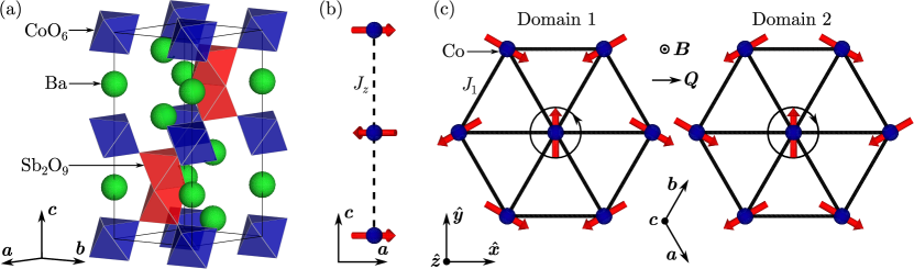
Figure 1: (Color online) (a) Crystal structure of Ba₃CoSb₂O₉ showing CoO₆ octahedra (blue) in the $ab$ plane separated by Ba²⁺ ions (green) and Sb₂O₉ double octahedra (red). There are two triangular CoO₆ layers in the structural hexagonal unit cell (thin outline) related by a two-fold screw axis around $c$. (b) Co²⁺ spins (red arrows) are ordered antiferromagnetically along $c$ due to the interlayer exchange $J_{z}$ (dashed line). (c) In the basal layers the ordered spins form a non-collinear $120^{\circ}$ structure and two possible magnetic domains are illustrated here. In domain 1 (left panel), the equilibrium spin direction rotates counterclockwise (sense indicated by the arrow on the circular envelope around the central site) between sites whose coordinate along the horizontal axis increases from left to right (along $\bm{a}+\bm{b}$) when viewed from above ($\bm{c}$ is out-of-page). In domain 2 (right panel), obtained from domain 1 by inversion on the central site, the rotation is in the opposite sense. Thick lines show the nearest neighbor $J_{1}$ exchange path. The in-plane projection of the propagation vector $\bm{Q}$ and the direction of the magnetic field $\bm{B}\parallel\bm{c}$ (for Section IV) are also indicated. The diagrams were produced using vesta.Momma and Izumi (2011)

Motivated by these open theoretical questions, we have revisited the magnetic excitations of Ba₃CoSb₂O₉, proposed to be one of the best realizations of a near-ideal spin-$\frac{1}{2}$ TLHAF with full three-fold lattice symmetry.Doi et al. (2004); Shirata et al. (2012); Zhou et al. (2012) The magnetic Co²⁺ ions are arranged in stacked triangular layers as per Fig. 1(a) (hexagonal space group $P6_{3}/mmc$ with lattice parameters $a=b=5.835$ Å and $c=14.448$ Å at 1.7 K). The combined effect of local octahedral crystal field and spin orbit coupling stabilize a Kramers doublet ground state with pseudospin $S=\frac{1}{2}$.Abragam and Pryce (1951) Magnetic order occurs below 3.8 K in a non-collinear $120^{\circ}$ structure [see Figs. 1(b)–(c)] with spins confined to the basal plane by a small easy-plane exchange anisotropy.Susuki et al. (2013); Koutroulakis et al. (2015); Quirion et al. (2015); Ma et al. (2016) The high symmetry of the crystal structure forbids Dzyaloshinskii-Moriya (DM) interactions between any pair of Co sites located in the same $ab$ plane or relatively displaced along the $c$ axis; thus DM interactions are ruled out on all the bonds that are most likely to carry significant exchange interactions. High-field measurements observed clear evidence for a one-third magnetization plateau for fields applied in the basal plane,Shirata et al. (2012); Susuki et al. (2013) as expected for the up-up-down phase stabilized by quantum fluctuations,Chubukov and Golosov (1991) a phase also observed in the spatially-anisotropic system Cs₂CuBr₄.Ono et al. (2003) Previous INS measurements in Ba₃CoSb₂O₉ revealed a strong downwards renormalization of the magnon dispersion, a pronounced roton-like minimum at the M points, and an extended scattering continuum at higher energies.Zhou et al. (2012); Ma et al. (2016); Ito et al. (2017) While the dispersion relations in the one-third magnetization plateau phase could be well described by a SWT$+1/S$ treatment for a spin Hamiltonian including easy-plane exchange anisotropy and interlayer couplings,Kamiya et al. (2018) the observed zero-field dispersions could not be quantitatively described even after including magnon interactions at order $1/S$ in SWT,Ma et al. (2016) suggesting that quantum renormalization effects in zero field are much stronger than in the one-third plateau phase and are underestimated by a perturbative SWT approach.

A quantitative parametrization of the dispersion relations and knowledge of the energy and wave vector dependence of the continuum scattering intensity are key pieces of information required by any theoretical models of the many-body quantum dynamics. Motivated by this, here we present extensive studies of the magnetic excitations in large single crystals of Ba₃CoSb₂O₉Prabhakaran and Boothroyd (2017) with high-resolution inelastic neutron scattering (INS) measurements spanning multiple Brillouin zones, which reveal that the high-energy excitation continuum displays highly-structured intensity modulations in momentum space with rings, hexagons and triangles apparent at various energies. Below the energy threshold of the continuum scattering, we observe sharp, resolution-limited magnons with no decay throughout the extended reciprocal space probed. We propose empirical wave vector-dependent renormalizations of the LSWT dispersion for a spin Hamiltonian with easy-plane exchange anisotropy, which allow us to quantitatively capture all modulations of the experimentally-observed magnon dispersion relations in the full three-dimensional Brillouin zone.

Our main results compared to previous studiesZhou et al. (2012); Ma et al. (2016); Ito et al. (2017) are i) the observation that magnons are sharp and do not decay throughout reciprocal space, and ii) a quantitative parametrization of the complete magnon dispersion relations in the full 3D Brillouin zone. For the observed strongly-renormalized dispersion, we find that one- and two-magnon phase spaces in energy and wave vector never overlap, so the magnon decays are in fact kinematically disallowed throughout the Brillouin zone, consistent with the experimental observation of sharp magnons throughout the probed reciprocal space. We note that while the absence of magnon decays cannot be understood within a SWT approach for the spin-$\frac{1}{2}$ TLHAF, it could in principle be explained if one assumes substantial easy-plane exchange anisotropy, which gaps out the primary one-magnon dispersion at the ordering wave vector and thus reduces very rapidly the overlap phase space, with no overlap expected for $\Delta\lesssim 0.92$ ($\Delta=1$ is the Heisenberg exchange limit). However, as pointed out by previous studies,Ma et al. (2016) the predicted magnon dispersions in this case of substantial easy-plane anisotropy are not compatible with the experimentally-observed dispersions. This suggests that quantum interaction effects between one-magnon and higher-energy continuum states in the actual material are significantly stronger than can be captured perturbatively by SWT at the $1/S$ level. This could be consistent with recent density matrix renormalization group (DMRG) calculations, which proposed avoided quasiparticle decay due to strong interactions in spin-$\frac{1}{2}$ models weakly perturbed away from the TLHAF limit.Verresen et al. (2019) Furthermore, we also observe direct evidence for a transfer of spectral weight from the one-magnon states to the higher-energy continuum, which may be understood (at least phenomenologically) as a further consequence of such strong interactions.

The rest of this paper is organized as follows. Section II describes the experimental setup used for the single-crystal INS measurements. The following section (Sec. III) presents the results for the magnetic excitations in the $120^{\circ}$ ordered state at low temperatures and zero applied magnetic field, starting in Sec. III.1 with an outline of the key features of the dispersion relations and the intensity modulations in the high-energy continuum scattering. Section III.2 reviews LSWT predictions of the magnon dispersions for a spin Hamiltonian with nearest-neighbor couplings and easy-plane exchange anisotropy. Section III.3 proposes empirical renormalizations of the analytic LSWT dispersion that can capture quantitatively the observed magnon dispersions in the full three-dimensional Brillouin zone and Sec. III.4 describes the fits to the INS data. Section III.5 verifies that one$\rightarrow$two magnon decays are kinematically disallowed for the parametrized one-magnon dispersion relation, thus providing a consistency check for the observation of sharp magnons with no decay throughout the reciprocal space probed. Section III.6 presents a quantitative comparison of the high-energy continuum scattering lineshapes with a two-magnon cross-section, highlighting which features can and which cannot be captured by such an approach. Section IV presents INS measurements of the spin dynamics in the cone phase in a $c$-axis magnetic field; the evolution of the dispersion relations with increasing field are in good (qualitative) agreement with a LSWT description when including symmetry-allowed magnetic domains with opposite senses of spin rotation in the $ab$ plane, as illustrated in Fig. 1(c). Finally, conclusions are summarized in Sec. V. The two appendices contain further technical details on the analysis. Appendix A presents LSWT calculations for the magnon dispersion relations and the one- and two-magnon dynamical structure factor, and sum rules for the total scattering used in the analysis to relate one- and two-magnon intensities. Appendix B presents analytic expressions for the wave vector and energy-dependent renormalizations used to parametrize the observed magnon dispersions.

II Experimental details

The spin dynamics of a sample of two co-aligned single crystals of Ba₃CoSb₂O₉, grown via the floating zone techniquePrabhakaran and Boothroyd (2017) (total mass 4 g), was measured using the direct-geometry time-of-flight neutron spectrometer LET at the ISIS neutron source in the UK.Bewley et al. (2011) For the zero-field measurements,Coldea et al. (2015) the sample was cooled by a variable-temperature insert with He⁴ exchange gas. Data were collected both at a base temperature of $1.7$ K, well below the magnetic ordering transition near $3.8$ K,Doi et al. (2004); Prabhakaran and Boothroyd (2017) and at $32$ K, deep in the paramagnetic phase. The spectrometer was operated in repetition rate multiplication (RRM) mode to collect the inelastic scattering simultaneously for monochromatic incident neutrons with energies $E_{\mathrm{i}}=3.53$ and 7.01 meV, with energy resolutions on the elastic line of 0.062(1) and 0.159(4) meV (full width at half maximum, FWHM), respectively. The first configuration provided high-resolution measurements of the magnon dispersions, which extend up to $\sim 1.6$ meV, whereas the second configuration probed the higher-energy scattering continuum extending up to at least 6 meV. The higher $E_{\mathrm{i}}$ data were normalized to give matching magnetic intensities to the lower $E_{\mathrm{i}}$ data in the overlapping region of energy transfers near $E\simeq 2$ meV, where the magnetic signal is a broad continuum in both wave vector and energy. The sample was mounted with the $c$ axis normal to the horizontal scattering plane, in order to probe the inelastic scattering in several Brillouin zones in the $hk0$ plane and (via scattering through the vertical opening of the magnet windows) access also more than a full Brillouin zone in the interlayer direction. The inelastic scattering was collected in Horace scans by rotating the sample around the vertical axis in an angular range of $140^{\circ}$ in steps of $0.5^{\circ}$. Counting times for each orientation were 15 minutes at the base temperature and 7 minutes in the paramagnetic phase, with an average proton current of 40 $\mu$A.

The same sample and a similar setup were used to measure the inelastic scattering in a magnetic field applied along the $c$ axis,Coldea et al. (2016) provided by a vertical 9 T cryomagnet. In this case, the sample was cooled using a dilution refrigerator and the inelastic scattering was measured at 3, 6 and 9 T at a base temperature of $0.1$ K. The spectrometer was operated in RRM mode for incident energies $E_{\mathrm{i}}=2.24$, 3.81 and 7.83 meV, with resolutions on the elastic line of 0.030(1), 0.064(1) and 0.179(8) meV (FWHM), respectively. Data were collected in Horace scans covering a similar range to zero-field measurements with coarser angular steps and average counting times of 8 minutes per orientation. The time-of-flight neutron data were processed using the mantidArnold et al. (2014) and horaceEwings et al. (2016) data analysis packages.

In order to maximize the counting statistics, for several of the plots in the paper the intensities were averaged between pixels from the full four-dimensional Horace scan with wave vector transfers $\bm{k}$ equivalent under symmetry operations of the crystal lattice point group ($6/mmm$). All those operations conserved $\lvert{\bm{k}}\rvert$, so the intensities of all averaged pixels had the same (spherical) magnetic form factor.

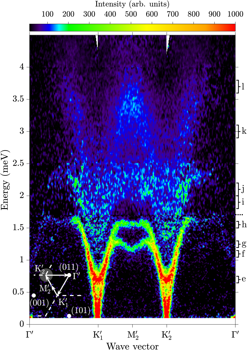
Figure 2: (Color online) Observed INS intensity ($1.7$ K) as a function of energy and wave vector transfer along a high-symmetry path in reciprocal space that crosses two magnetic Bragg peak positions (K${}^{\prime}_{1,2}$). The color shows the raw neutron counts in arbitrary units. Two sharp magnon dispersion branches are clearly observed, accompanied by a strong scattering continuum with a structured intensity pattern. The brackets on the right-hand side labeled (e)-(l) indicate the energy integration ranges for the $hk$ slices with the same panel labels plotted in Fig. 3. The wave vector path is $\Gamma^{\prime}\,(0,1,1)\rightarrow\mathrm{K}^{\prime}_{1}\,(\frac{1}{3},\frac{1}{3},1)\rightarrow\mathrm{M}^{\prime}_{2}\,(0,\frac{1}{2},1)\rightarrow\mathrm{K}^{\prime}_{2}\,(-\frac{1}{3},\frac{2}{3},1)\rightarrow\Gamma^{\prime}$, illustrated by arrows in the white bottom-left inset with the Brillouin zone boundaries represented by dashed lines. The data below 0.1 meV has been omitted as it is dominated by incoherent quasielastic scattering. The data up to 1.7 meV (horizontal dotted line on the right-hand side) was collected using $E_{\mathrm{i}}=3.53$ meV, and at higher energies with $E_{\mathrm{i}}=7.01$ meV, scaled as described in the text. The wave vector integration range in the $hk$ plane is $\pm 0.05$ Å^-1, and along $l$ is $\pm 0.05$ Å^-1 for energies $E\leq 2$ meV, $\pm 0.1$ Å^-1 for $2<E\leq 4$ meV and $\pm 0.2$ Å^-1 for $E>4$ meV.

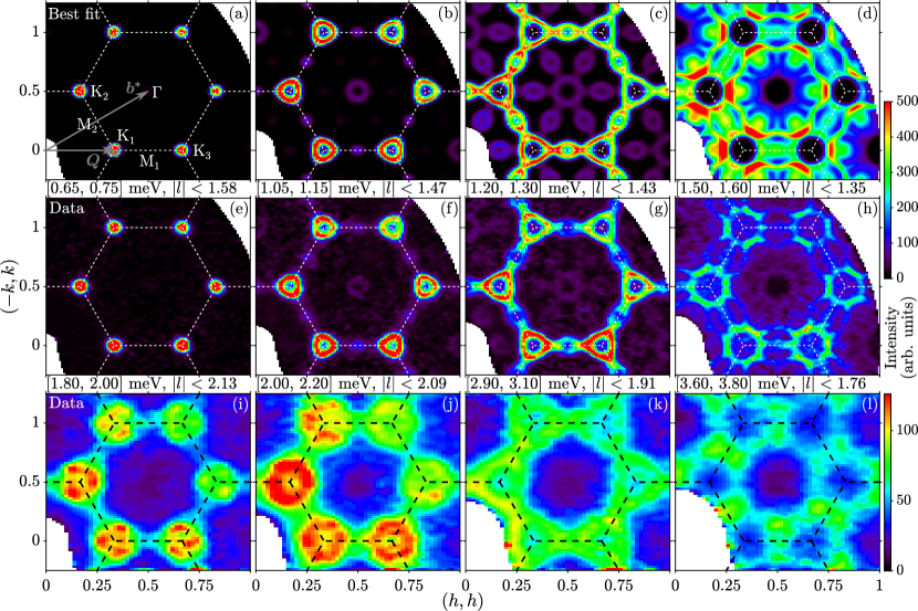
Figure 3: (Color online) INS intensity maps as a function of momentum in the $hk$ plane at a series of constant energies, compared with model calculations. (e)–(h) Intensity maps up to 1.6 meV showing constant-energy contours of the one-magnon dispersions. (a)–(d) Corresponding calculations for the best-fit spin wave model with renormalized dispersions described in the text. The model is the one-magnon cross-section, including the magnetic form factor for Co²⁺ ions, the neutron polarization factor, the finite-temperature Bose factor and convolution with the instrumental resolution (for details see Appendix A). (i)–(l) Intensity maps through the continuum scattering at higher energies (above 1.8 meV). The data were collected at 1.7 K with $E_{\mathrm{i}}=3.53$ meV for (e)–(h) and 7.01 meV for (i)–(l). In all data panels, the color shows the raw neutron counts in arbitrary units. In all panels, dashed lines indicate hexagonal Brillouin zone boundaries. In panel (a), gray arrows show the projections of $\bm{b}^{\ast}$ and $\bm{Q}$ wave vectors, and labels K${}_{1\text{--}3}$, M_1,2 and $\Gamma$ indicate high-symmetry points referred to in the rest of the paper. The energy integration ranges of the data panels are given in the panel titles and also indicated by the labeled brackets on the right of Fig. 2.

III Spin dynamics in zero field

III.1 Key features of the magnon dispersions and continuum scattering

We begin by presenting the results for the spin dynamics in zero applied field at a base temperature of $1.7$ K. It is well established experimentallySusuki et al. (2013); Koutroulakis et al. (2015); Quirion et al. (2015); Ma et al. (2016) that the magnetic structure in the ground state has spins ordered at $120^{\circ}$ relative to nearest-neighbor sites in the triangular layers, as illustrated in Fig. 1(c), and antiparallel between adjacent layers stacked along $c$, see Fig. 1(b). Compared to the structural unit cell, the magnetic unit cell is tripled in the $ab$ plane, but is the same length along $c$, with two triangular layers per unit cell. The magnetic structure can be described in terms of a single propagation vector $\bm{Q}=(\frac{1}{3},\frac{1}{3},1)$, where throughout we index wave vectors in terms of reciprocal lattice units ($h,k,l$) of the hexagonal structural unit cell. The in-plane components of $\bm{Q}$ capture the $120^{\circ}$ order in a single layer and the out-of-plane component captures the antiferromagnetic order between layers spaced by $c/2$. In the absence of DM interactions, the two senses of spin rotation in the triangular layers [counterclockwise/clockwise illustrated in Fig. 1(c) left/right panels] are degenerate, so one expects a macroscopic sample to contain magnetic domains of both types. In the absence of bond-dependent spin-exchange anisotropies, believed to be negligible here, the two magnetic domains have identical excitation spectra in zero field. (We will show later in Sec. IV that the two domains have different spectra in a finite $c$-axis magnetic field.)

An overview of the observed excitation spectrum as a function of energy and wave vector is shown in Fig. 2 along a representative path in reciprocal space. Throughout this paper, wave vector labels $\Gamma$, M and K refer to the conventional high-symmetry points in the two-dimensional (2D) hexagonal Brillouin zone, where an unprimed (primed) label indicates $l=0$ ($l=1$) and numbered subscripts (as in M_1,2) refer to distinct points in reciprocal space that are related by a symmetry operation of the lattice point group when reduced to the first Brillouin zone. Figure 2 shows that the inelastic scattering intensity is strongest near the magnetic Bragg wave vectors K${}_{1,2}^{\prime}$, and two sharp, well-defined magnon branches are clearly resolved: one gapless and linearly dispersing at low energies, and the other one gapped ($E_{\mathrm{gap}}\simeq 0.7$ meV) at the magnetic Bragg position. These modes correspond to the gapless Goldstone mode associated with rotation of the spins in the $ab$ plane and an out-of-plane mode that is gapped in the presence of easy-plane (exchange) anisotropy, respectively. In the center of the figure at the M${}^{\prime}_{2}$ point, there is a clear local minimum (roton-like soft mode) in the lower dispersive branch, where the energy is $\sim$8% lower compared to that of the nearby local maximum in that branch; a flattening of the dispersion and a less pronounced soft mode ($\sim$1% relative dip) is also visible in the top branch. We will refer to these later as the lower/higher soft modes, respectively. At the energies of the soft modes, there is almost no detectable dispersion along the interlayer direction, so we regard these soft modes as a consequence of the two-dimensional physics in the triangular layers.

Important features of the dispersions are also highlighted in constant-energy intensity maps. In particular, the triangular-shaped contours with 3-fold rotational symmetry around the Brillouin zone corners in Figs. 3(f),(g) are characteristic of the spin wave dispersion shape on the triangular lattice, and the oval-shaped contours near the mid-points of the zone in Fig. 3(g) are due to the soft mode at M points in the lower magnon mode. Returning to Fig. 2, there is considerable inelastic signal above the sharp magnon dispersions in the form of a highly-structured continuum, present already inside the magnon dispersion cones (emerging out of the magnetic Bragg peaks) and extending higher in energy up to at least 6 meV (data shown up to 4.5 meV in Fig. 2). The continuum intensity is strongly modulated in both energy and wave vector. This is clearly illustrated in the intensity maps at constant energy in Figs. 3(i)–(l). At energies just above the top of the one-magnon dispersions [panel (i)], the continuum intensity is strongest above the magnon cones centered at K points with a clear 3-fold symmetric pattern. At slightly higher energies [panel (j)], ring patterns around K become apparent, and these transform [in panel (k)] into triangular contours with corners touching at M points. At even higher energies [panel (l)], the signal near M points has spread out in the direction normal to the Brillouin zone edges, such that the intensity is strongest along hexagonal contours centered at $\Gamma$ and connected across M points between adjacent Brillouin zones. All the above features become overdamped in the paramagnetic phase at 32 K (not shown), confirming their magnetic character.

III.2 Magnon dispersions within linear spin wave theory

To parametrize the dispersion relations, following previous studiesSusuki et al. (2013); Ma et al. (2016) we consider the minimal spin Hamiltonian

$$\mathcal{H} =J_{1}\sum^{\mathrm{NN}}_{\langle{ij}\rangle}S^{x}_{i}S^{x}_{j}+S^{y}_{i}S^{y}_{j}+\Delta{}S^{z}_{i}S^{z}_{j}$$

$$+J_{z}\sum^{\mathrm{interlayer}}_{\langle{mn}\rangle}S^{x}_{m}S^{x}_{n}+S^{y}_{m}S^{y}_{n}+\Delta{}S^{z}_{m}S^{z}_{n},$$ (1)

where the nearest-neighbor (NN) intralayer exchange $J_{1}$, the interlayer exchange $J_{z}$ (both antiferromagnetic), and the orientation of the ($x,y,z$) axes are all illustrated in Figs. 1(b)–(c). $\Delta<1$ parametrizes the easy-plane exchange anisotropy. This spin Hamiltonian has continuous rotational symmetry about the $z$ axis in spin space. The crystal structure however has only discrete rotational symmetries, so we have neglected in the above Hamiltonian symmetry-allowed bond-dependent exchange anisotropy terms, such as different exchange couplings for the in-plane spin components along and perpendicular to a NN bond.

The mean-field ground state of the Hamiltonian in Eq. (1) has $120^{\circ}$ spin order in the layers and AFM stacking along $c$, as illustrated in Figs. 1(b)–(c). The derivation of the dispersion relations and dynamical structure factor within LSWT is reviewed in Appendix A. Three magnon modes are expected for a general wave vector $\bm{k}$: a primary mode $\omega(\bm{k})$ and two secondary modes $\omega^{\pm}(\bm{k})\equiv\omega(\bm{k}\pm\bm{Q})$, where $\bm{Q}$ is the propagation vector of the magnetic structure. For a given wave vector $\bm{k}$, in general only two out of the three modes carry significant weight (for the dynamical structure factor calculation see Appendix A).

We discuss below the key properties of the primary mode, as the secondary modes are easily obtained by wave vector translations. The primary mode is gapless at the origin $\bm{k}=\bm{0}$, corresponding to the Goldstone mode of spin rotations in the $xy$ plane. For finite easy-plane anisotropy ($\Delta<1$), the primary mode has a gap at the magnetic Bragg peak positions $\bm{k}=\pm\bm{Q}$ of magnitude $E_{\mathrm{gap}}=3\sqrt{3/2}\>J_{1}S\sqrt{1-\Delta}$ for $J_{z}=0$. The interlayer coupling $J_{z}$ leads to a finite dispersion along $l$ with a zone boundary energy at $(001)$ of magnitude $6S\sqrt{J_{1}J_{z}}$ for $\Delta=1$. Previous studiesMa et al. (2016); Ito et al. (2017) have shown that LSWT for the above spin Hamiltonian can be used to parametrize well the low-energy dispersions in Ba₃CoSb₂O₉ up to an energy of the order of the interlayer zone boundary energy. However the dispersions at higher energies, in particular close to the top of the dispersions, could not be accounted for.Ma et al. (2016) Even when including magnon interaction effects to order $1/S$, the maximum magnon energy was overestimated by about 45%, suggesting that quantum renormalization effects on the magnon dispersions are stronger than can be captured perturbatively at order $1/S$ in SWT. In the following, to make progress we propose an empirical parametrization of the dispersion relations.

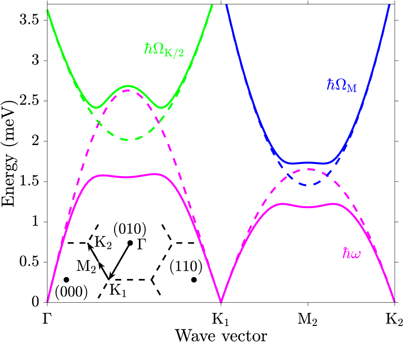
Figure 4: (Color online) Illustration of the renormalizations applied to the bare LSWT dispersion in order to capture the experimental magnon dispersion. For simplicity, all calculations are for the special case of the isotropic 2D TLHAF model ($J_{z}=0,\Delta=1$). Dashed magenta lines show the bare dispersion $\hbar\omega_{\mathrm{LSWT}}$ in Eq. (4) plotted along a high-symmetry path in the Brillouin zone [schematically shown in the bottom left inset]. The soft modes at M and near K/2 are introduced by adding a virtual interaction with fictitious parabolic modes $\hbar\Omega_{\mathrm{M}}$ (blue dashed line) and $\hbar\Omega_{\mathrm{K/2}}$ (green dashed line). The resulting renormalized dispersion $\hbar\omega$ (solid magenta line) is fitted to the experimental magnon dispersion.

III.3 Proposed empirical parametrization of the observed magnon dispersions

From general arguments, one expects that the physical magnon dispersion would satisfy the same periodicity in reciprocal space and the same lattice point group symmetries as the LSWT dispersion, but that it may be squeezed, stretched or otherwise deformed compared to the LSWT prediction at various momenta and/or energies. In this spirit, we introduce below wave vector-dependent renormalizations that preserve the lattice point group symmetries and allow us to quantitatively capture all dispersion modulations in the full three-dimensional Brillouin zone. All operations are performed on the primary magnon dispersion, as the secondary modes are obtained simply by a wave vector shift. The complete analytical forms of the renormalization functions used are given in Appendix B; here we discuss their physical motivation and qualitative features.

Wave vector dependent modifications are introduced to reproduce the local minima (soft modes) observed in Fig. 2 near the M${}_{2}^{\prime}$ point. The lower soft mode occurs in the primary magnon dispersion. LSWT predicts a saddle point at this position with a local maximum in the M-K direction and a local minimum in the M-$\Gamma$ direction, see Fig. 5(a). In order to obtain a local minimum in both in-plane directions, we consider in Fig. 4 the mixing of the bare dispersion $\hbar\omega_{\mathrm{LSWT}}$ (dashed magenta line) with a fictitious gapped mode $\hbar\Omega_{\mathrm{M}}$ (dashed blue line) centered at M and parabolic in the $hk$ plane; the resulting lower mode after mixing (magenta solid line) has the desired qualitative feature of a smooth local minimum at M. To parametrize the upper soft mode visible in Fig. 2 near M${}_{2}^{\prime}$, we first note that this feature occurs in the secondary modes $\omega^{\pm}(\bm{k})$, which nearly overlap in this wave vector region and furthermore trade intensity with each other, such that effectively a single higher-energy magnon branch is visible. The corresponding location in reciprocal space where the primary mode would display such a soft mode is near $\bm{k}_{\mathrm{M}}\pm\bm{Q}$, symmetry equivalent to $\bm{Q}/2$, i.e. located half-way between $\Gamma$ and K; we will refer to this as K/2 from now on (in the notation of the theoretical references Verresen et al., 2019 and Ferrari and Becca, 2019, this is the Y₁ point). We illustrate in Fig. 4 the procedure to obtain a local soft minimum via mixing with a virtual parabolic mode $\hbar\Omega_{\mathrm{K/2}}$ centered near K/2 (dashed green line); the lower mode after mixing (magenta solid line) displays the desired local soft mode feature. To obtain the “final” renormalized dispersion $\hbar\omega$ that was fitted to the data, $\hbar\omega_{\mathrm{LSWT}}$ was mixed with many virtual paraboloids at equivalent M and K/2-type positions (up to reciprocal lattice translations or lattice point group symmetry operations) at the same $l$ value, in order to ensure the final result is a smooth function that still respects all lattice point group symmetries. Figure 5(b) shows a contour map of the renormalized dispersion surface in the $(hk0)$ plane, which highlights the location of soft modes at M and near K/2 points, not present for the bare $\hbar\omega_{\mathrm{LSWT}}$ dispersion in panel (a).

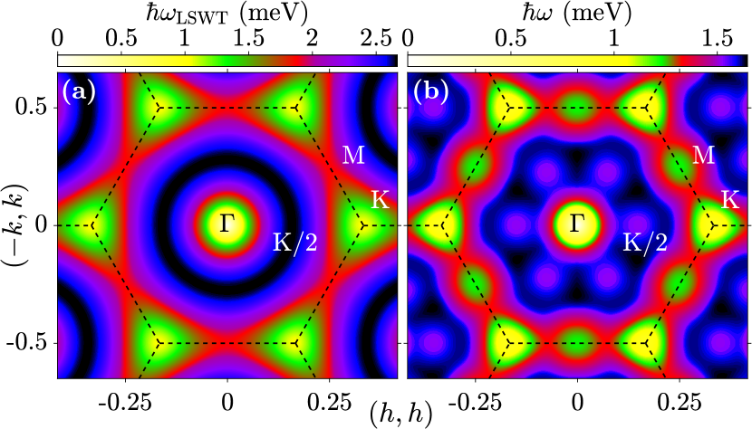
Figure 5: (Color online) (a) Contour map in the $(hk0)$ plane of (a) the LSWT dispersion $\hbar\omega_{\mathrm{LSWT}}(\bm{k})$ and (b) the best-fit renormalized dispersion $\hbar\omega(\bm{k})$, using parameters in Table 1 in Appendix B. Dashed lines show the hexagonal Brillouin zone boundaries. The separate color maps in the two panels highlight relevant features of the two distinct dispersion surfaces. The maximum in $\hbar\omega_{\mathrm{LSWT}}(\bm{k})$ occurs on a circle centered at $\Gamma$ and passing near the six K/2 wave vectors; this is replaced in the renormalized dispersion by a near-plateau in a wide annular region with shallow local minima near the set of six K/2 points. $\hbar\omega_{\mathrm{LSWT}}(\bm{k})$ has saddle points at the M zone-boundary points, whereas at those positions the renormalized dispersion $\hbar\omega$ has oval-shaped local minima. The triangular-shaped contours around K and oval-shaped ones around M in (b) are clearly visible in the constant-energy INS intensity map in Fig. 3(g).

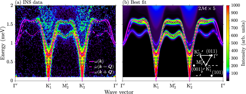
Figure 6: (Color online) Comparison of (a) INS data (1.7 K, $E_{\mathrm{i}}=3.53$ meV) with (b) the best-fit spin wave model with renormalized dispersions, along a high-symmetry path in the $(hk1)$ plane crossing two magnetic Bragg peaks at K${}_{1,2}^{\prime}$. The color in (a) shows the raw neutron counts in arbitrary units. The calculation in (b) includes both the one-magnon and two-magnon ($2{\mathcal{M}}$) cross-sections (the latter multiplied by a factor of 5 for better visibility). The white circles in (a) are experimental dispersion points (error bars smaller than the size of symbols), extracted by fitting Gaussian peaks to constant energy or constant wave vector scans through the sharp modes; their positions are well described by the model dispersions, shown by the solid, dashed and dotted magenta lines for the $\omega(\bm{k})$, $\omega(\bm{k-Q})$ and $\omega(\bm{k+Q})$ modes, respectively. The wave vector path is $\Gamma^{\prime}\,(0,1,1)\rightarrow\mathrm{K}^{\prime}_{1}\,(\frac{1}{3},\frac{1}{3},1)\rightarrow\mathrm{M}^{\prime}_{2}\,(0,\frac{1}{2},1)\rightarrow\mathrm{K}^{\prime}_{2}\,(-\frac{1}{3},\frac{2}{3},1)\rightarrow\Gamma^{\prime}$, illustrated by thick arrows in the white bottom-right inset with the Brillouin zone boundaries represented by dashed lines. The integration width for the data in the $hk$ plane is $\pm 0.05$ Å^-1 and along $l$ is $\pm 0.05$ Å^-1. The quasielastic scattering below 0.1 meV has been omitted.

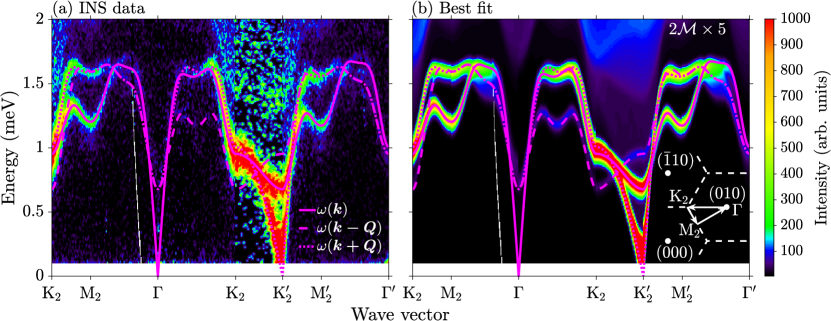
Figure 7: (Color online) Same as Fig. 6, but for a wave vector path that probes the interlayer $l$ dispersion: $\mathrm{K}_{2}\,(-\frac{1}{3},\frac{2}{3},0)\rightarrow\mathrm{M}_{2}\,(0,\frac{1}{2},0)\rightarrow\Gamma\,(0,1,0)\rightarrow\mathrm{K}_{2}\rightarrow\mathrm{K}^{\prime}_{2}\,(-\frac{1}{3},\frac{2}{3},1)\rightarrow\mathrm{M}^{\prime}_{2}\,(0,\frac{1}{2},1)\rightarrow\Gamma^{\prime}\,(0,1,1)$, illustrated in the white bottom-right inset. The integration width in the $hk$ plane is $\pm 0.05$ Å^-1 for panels 1–3 and 6, and $\pm 0.02$ Å^-1 for panels 4 and 5, and along $l$ is $\pm 0.1$ Å^-1 for panels 1, 3 and 5, and $\pm 0.3$ Å^-1 for panels 2 and 6.

III.4 Fits of INS data to the spin wave model with renormalized dispersions

The above spin wave model with renormalized dispersions was fitted to the experimental data as follows. First, an initial parametrization of the dispersion relation was obtained by fitting the functional form of the renormalized spin wave dispersion to a set of $(h,k,l,E)$ dispersion points, extracted by fitting Gaussian peaks to constant energy or constant wave vector scans through the INS data in regions where the magnon modes were clearly separated from one another and where the character of each mode [whether $\omega(\bm{k})$, $\omega^{+}(\bm{k})$ or $\omega^{-}(\bm{k})$] could be unambiguously identified from the dispersion trends. This dispersion parametrization was then used as a starting point and further refined by performing a global fit of the full one-magnon cross-section model, including all three magnon branches, to selected slices and cuts through the four-dimensional INS data along many symmetry-distinct directions in reciprocal space (representative slices shown in Figs. 6 and 7). To ensure the model fitted only the one-magnon intensity data, the regions with clear continuum scattering in those slices were masked in the fit; for example, data pixels contributing to the gapped “cones” of continuum scattering at high energies near K_1,2 points in Fig. 6(a) were excluded from the fit. The one-magnon cross-section model included the effects of the finite-temperature Bose factor, the magnetic form factor for Co²⁺ ions, the neutron polarization factor, and a parametrization of the exprimental energy resolution (for details, see Appendix A). The linewidth of the observed sharp one-magnon modes in constant wave vector scans was well accounted for by the parametrized instrumental energy resolution, suggesting that the magnons are long-lived with no evidence of lifetime broadening. Model parameters obtained through this fitting procedure are listed in Table 1 (Appendix B) and include the two exchange parameters $J_{1}$ and $J_{z}$, the exchange anisotropy $\Delta$, the relative in-plane/out-of-plane magnon intensity prefactor $Z_{\eta}/Z_{\xi}$, and parameters to describe the two types of soft modes at M and near K/2. The Hamiltonian parameters were constrained to reproduce the observed magnetization saturation fieldKamiya et al. (2018)

$$g\mu_{\rm{B}}B_{\rm sat}S^{-1}=(3+6\Delta)J_{1}+2(1+\Delta)J_{z},$$ (2)

with $B_{\rm sat}=32.8$ T and $g$ factor $g=3.87$.

This model provides an excellent description of the experimental dispersion relations at all energies and wave vectors probed, as illustrated by comparing (a) the data and (b) the parametrization plots in Fig. 6 for wave vector directions in the $(hk1)$ plane and Fig. 7 for wave vectors also probing the interlayer $l$ dispersions. Open white circles in Fig. 6(a) correspond to empirical peak centers extracted from Gaussian fits to constant energy or constant wave vector scans; their close agreement with the overplotted dispersion relations (magenta lines) emphasises the level of quantitative agreement between data and model. All key features of the dispersion are quantitatively reproduced, including the energy of the gapped mode at the magnetic Bragg peak positions K${}_{1,2}^{\prime}$, the dispersion along the interlayer K₂-K${}^{\prime}_{2}$ direction in Fig. 7, the relative flattening of the dispersions near the maximum energy, and the dispersion shapes near the soft modes at M and near K/2 points.

Although the present analysis focuses on capturing the intermediate to high-energy features of the dispersions, where the spin wave peaks are most accurately determined experimentally as they are well separated in energy and momentum, the parametrization also captures well the low-energy behavior. In particular, the steep linearly-dispersive spin wave cones emerging out of the magnetic Bragg peak positions K${}_{1}^{\prime}$ and K${}_{2}^{\prime}$ in Fig. 6, attributed to the gapless $\omega^{-}(\bm{k})$ and $\omega^{+}(\bm{k})$ modes, respectively, are consistent between the data and the model parametrization. We note however that the spin wave peaks are barely resolved at low energies due to the very steep dispersion combined with the finite instrumental resolution, so changes in the spin wave velocity of order $10\%$ compared to the LSWT result as predicted by SWT$+1/S$ treatmentsChubukov et al. (1994) could also be consistent with the data in this low-energy region. Testing quantitatively for such spin wave renormalization effects in the limit $\omega\rightarrow 0$ would require a more sophisticated analysis, including theoretical predictions of the complete wave vector and energy-dependent quantum renormalization of the dispersions and intensities for the full Hamiltonian in Eq. (1), which is beyond the scope of the present empirical parametrization.

Turning now to the magnon intensities, the strongest signal in Figs. 6 and 7 is observed near K points with intensities decreasing rapidly approaching the $\Gamma$ points, and this general trend is well reproduced by the model. However, close inspection of the intensity variation, in particular as a function of energy, reveals a discrepancy between the data and model; namely, if the overall intensity scale in the calculation is set to match the intensities of the low-energy magnons in those figures, then the intensity of the high-energy magnons is much lower in the data than in the calculation, compare Fig. 6(a) with (b), also Fig. 7(a) with (b), and Fig. 3(h) with (d). (Unless otherwise specified, the overall intensity scale is chosen to match the observed low-energy signal for all calculated intensity color maps throughout the paper.) We propose that this discrepancy between the spin wave model and data is evidence of a transfer of spectral weight from the one-magnon modes to the higher-energy continuum scattering that is not captured by the model; such a transfer of spectral weight is expected from general considerations as a consequence of the interaction between the high-energy magnons and the higher-energy continuum states, expected to result in a downward renormalization of the magnon energies and a simultaneous transfer of intensity from the high-energy magnons to the continuum states. Further support for this interpretation will be provided later in Section III.6, where we compare directly the observed scattering lineshapes with predictions of the spin wave model for both one- and two-magnon excitations.

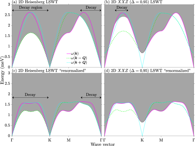
Figure 8: (Color online) Phase space (shaded area) for two-magnon excitations along high-symmetry wave vector directions, compared with the one-magnon dispersion relation $\hbar\omega(\bm{k})$ (magenta solid line). When overlap occurs, magnons are unstable to decay, and those regions are indicated by the horizontal double-arrowed lines labeled “Decay”. The four figure panels correspond to different two-dimensional spin wave models related to the Hamiltonian in Eq. (1) with $J_{z}=0$. (a) 2D Heisenberg ($\Delta=1$) model within LSWT, for which decay is expected along the whole $\Gamma$-K line and also a finite wave vector range starting from $\Gamma$ towards M. (b) Easy-plane XXZ ($\Delta=0.95$) model within LSWT, where the anisotropy opens a gap at K. The phase space for magnon decay is much reduced compared to (a), but is still present near the top of the $\Gamma$-K dispersion. (c) and (d) are the same as (a) and (b), but with the empirical renormalizations applied to the LSWT dispersions, as described in Sec. III.3. In (c) the renormalizations have not greatly affected the decay regions compared to (a), whereas in (d) the decay regions are completely eliminated, meaning magnons are sharp everywhere. The exchange and dispersion renormalization parameters used are listed in Table 1 in Appendix B. As explained in the text, the plots are for the rotating reference frame, where a single magnon mode is present with dispersion $\hbar\omega(\bm{k})$.

III.5 Why are magnons sharp and do not decay?

We find experimentally that the magnons are sharp, with resolution-limited lineshapes throughout the extensive region of reciprocal space probed with no evidence of intrinsic broadening, indicating that magnon decay processes do not occur. This is a non-trivial result, as SWT+$1/S$ theoretical studies have predicted extended regions of one$\rightarrow$two magnon decays for the spin-$\frac{1}{2}$ TLHAF limit.Mourigal et al. (2013) We review below the requirements for magnon decays following Ref. Chernyshev and Zhitomirsky, 2009 and find that they are not satisfied in Ba₃CoSb₂O₉. In particular, we find that the shape of the magnon dispersion is quite different from that of the TLHAF model and is such that overlap between one- and two-magnon phase spaces is avoided throughout reciprocal space, so no decay can occur.

Specifically, decay processes require that (i) the spin Hamiltonian has finite matrix elements for mixing between one- and two-magnon states, and (ii) energy and momentum are conserved during the decay, i.e. a magnon at wave vector $\bm{k}$ can kinematically decay into a pair of magnons with wave vectors $\bm{k}_{1}$ and $\bm{k}_{2}$ if

$$\bm{k}=\bm{k}_{1}+\bm{k}_{2}\quad\mathrm{and}~{}~{}\omega(\bm{k})=\omega(\bm{k}_{1})+\omega(\bm{k}_{2}).$$

The finite matrix element requirement for decay is naturally satisfied due to the non-collinear nature of the $120^{\circ}$ order in the ground state, which leads to couplings between longitudinal spin fluctuations on one site and transverse fluctuations on neighboring sites (defining longitudinal and transverse as along and perpendicular to the local ordered spin direction, respectively), which in turn mixes one- and two-magnon states.Chernyshev and Zhitomirsky (2009) The kinematic constraint is most transparently tested by working in the rotating reference frame that follows the local ordered spin orientation, in which the ground state is ferromagnetic and there is a single magnon mode with dispersion $\omega({\bm{k}})$ (for more details see Appendix A). The phase space of two-magnon excitations in this rotating frame is illustrated by the shaded area in Fig. 8(a) for the 2D Heisenberg model described within LSWT. Decay is expected where the one-magnon dispersion (magenta solid line) overlaps with the shaded area, which occurs throughout the $\Gamma$-K line and over a significant portion of the $\Gamma$-M line. In addition to the magnon dispersion $\omega({\bm{k}})$, the figure also shows the wave vector shifted dispersions $\omega({\bm{k}\pm\bm{Q}})$ (dotted green/dashed cyan lines), which helps to emphasize that the lower boundary of the two-magnon continuum at a fixed wave vector $\bm{k}$ is the minimum energy of those three curves. This occurs because the lower boundary corresponds to creating one of the two magnons at zero energy at either the $\Gamma$ point ($\bm{k}_{1}=\bm{0}$) or at one of the two K points ($\bm{k}_{1}=\mp\bm{Q}$), thus placing the other magnon in the pair at wave vector $\bm{k}_{2}=\bm{k}$ with energy $\omega(\bm{k})$ or at $\bm{k}_{2}=\bm{k}\pm\bm{Q}$ with energy $\omega(\bm{k}\pm\bm{Q})$, respectively. If an easy-plane anisotropy is added, as in Fig. 8(b), the dispersion becomes gapped at the ordering wave vector (K points), which increases the minimum energy cost of creating two-magnon states and therefore reduces the regions of overlap between one- and two-magnon states. Despite this, a finite decay region is still expected near the top of the $\Gamma$-K dispersion, if the dispersion shape is given by the LSWT result.

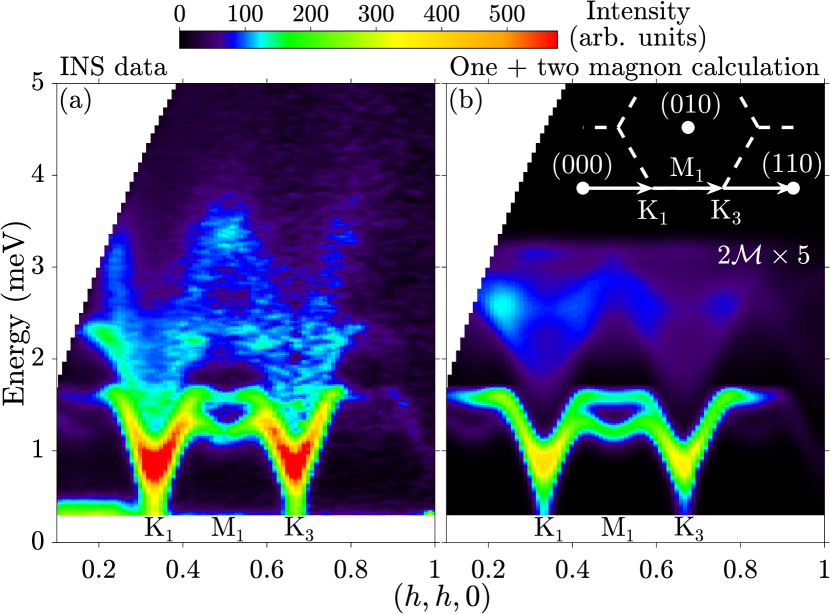
Figure 9: (Color online) (a) INS data (1.7 K, $E_{\mathrm{i}}=7.01$ meV) showing the full extent of the magnetic excitation spectrum, compared in (b) with the renormalized spin wave model. The wave vector path is $(h\mp 0.05,h\pm 0.05,\pm 2.39)$, where the $\pm$ signs indicate the data integration range. The color shows the raw neutron counts in arbitrary units. The calculation in (b) includes both the one-magnon and two-magnon ($2{\mathcal{M}}$) cross-sections (the latter multiplied by a factor of 5 for better visibility). The intensity scale factor in (b) is chosen to reproduce the observed intensities of the sharp magnons near M₁ in (a).

The above analysis is however oversimplified, as the experimental dispersion relations are in fact strongly renormalized in non-trivial ways compared to the LSWT prediction, as found in the preceding Sec. III.4. This is physically attributed to the effect of magnon interactions and quantum fluctuations beyond the linear spin wave approximation. In Fig. 8(c), the solid magenta line is the dispersion relation from (a) after applying the same wave vector-dependent renormalizations as for the full model fitted to the experimental data, using the parameters in Table 1 but with $J_{z}=0$ and $\Delta=1$. In other words, we assume that the empirically-determined dispersion renormalizations are unaffected by the weak 3D couplings and the small easy-plane anisotropy. Figure 8(c) shows that the overlap regions are not changed much by these renormalizations and so extended decay regions are predicted. Finally, in Fig. 8(d) we consider a spin wave model with finite easy-plane anisotropy and dispersion renormalizations included, which is closer to experimental observations. In this case, we find that the magnon dispersion $\omega(\bm{k})$ defines the lower boundary of the two-magnon continuum but never enters it, so decay regions are completely eliminated. For finite values of the interlayer coupling $J_{z}$ that are consistent with the experimental data, there are only very small changes to cases (c) and (d) and the qualitative content is unaffected, i.e. extended decay regions are still present in (c) but remain absent in (d). As the 3D couplings have only very small effects on the magnon decay regions, panel (d) captures the essential physics of avoided magnon decays in the present system.

The above analysis of the different models suggests that magnon decays do not occur in Ba₃CoSb₂O₉ because of the combined effect of the small, but finite easy-plane anisotropy ($\Delta<1$) and the strong dispersion renormalizations from quantum effects, with both effects playing a rôle.

We note that recent theoretical work,Verresen et al. (2019) based on DMRG calculations for gapped spin models models slightly perturbed away from the TLHAF limit, proposed that strong quantum interactions lead to an avoidance of the LSWT-predicted overlap between the one-magnon dispersion and the higher-energy two-magnon continuum scattering; the resulting magnon dispersion is renormalized downwards and has a much reduced spectral weight, due to a transfer of weight to the higher-energy continuum states via the aforementioned interactions. It would be interesting if such calculations could be extended to the weak easy-plane anisotropy case relevant here where the spectrum is gapless, and also much closer to the isotropic Heisenberg limit, to test if the same picture applies. In addition, recent variational dynamical Monte Carlo calculations proposed that magnons remain sharp throughout the Brillouin zone in the fully isotropic Heisenberg limit.Ferrari and Becca (2019)

III.6 Continuum scattering compared with a two-magnon cross-section

An overview of the complete magnetic excitation spectrum is plotted in Fig. 9(a). Sharp spin wave modes are visible up to 1.6 meV, followed by a continuum of scattering, which appears to emerge from inside the spin wave cones centered at wave vectors K_1,3 and extends in energy up to at least the top of the plotted range. Inside the continuum, highly-dispersive intensity modulations are clearly visible, in the form of two successive cones of intensity in different energy ranges, both centered at the K points and dispersing in energy with maxima at M points. Panel (b) shows the corresponding calculation for the best-fit renormalized spin wave model. The magnon dispersions are well captured, but the predicted two-magnon (2$\mathcal{M}$) continuum (shown with intensity scaled up by a factor of 5 for visibility) is not able to account for the large scattering weight in the experimentally observed continuum. Nor can it explain the highly-structured intensity modulations, predicting just one filled cone of intensity centered at K points and dispersing in energy up to M, shifted in energy compared to the experimentally-observed intensity modulations in panel (a).

Figure 10(a) presents a quantitative data vs. model lineshape comparison for an energy scan at a wave vector equivalent to M₁ [near the center of Fig. 9(a)]. The two sharp peaks on the low-energy side are well accounted for by resolution-limited magnons, where the first peak is identified with the out-of-plane $\omega({\bm{k}})$ mode and the second with degenerate in-plane $\omega^{\pm}(\bm{k})$ magnons. However, the large continuum scattering at higher energies (emphasized by the gray shading) is much underestimated by the two-magnon cross-section (pink shading). (For details of the calculation, see Appendix A.) Note that the two prominent broad peaks in the continuum near 2.3 and 3.5 meV correspond to the two broad intensity maxima near the center of Fig. 9(a).

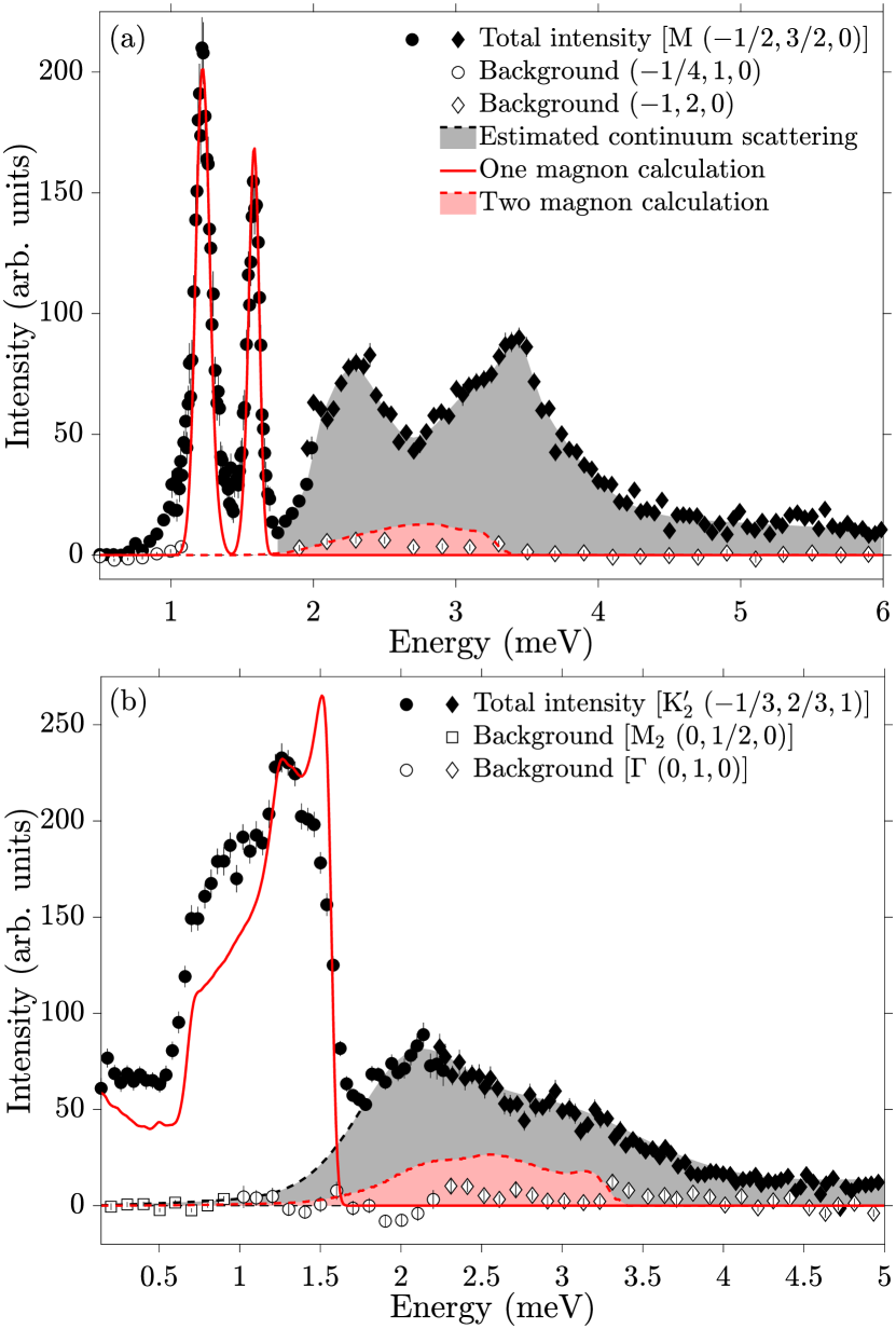
Figure 10: (Color online) Energy scans through the INS data (filled symbols, 1.7 K) (a) at an M zone boundary point [equivalent to M₁ in Fig. 9(a)] and (b) near a magnetic Bragg wave vector (K${}_{2}^{\prime}$ in Fig. 2), compared with the renormalized spin wave model (red line and pink shading represent one-magnon and two-magnon excitations, respectively). Data points are raw neutron counts with an estimate of an energy-dependent non-magnetic background subtracted. The accuracy of the background subtraction is illustrated by the open symbols, which show the resulting intensities in regions of wave vector and energy where no magnetic scattering is expected. Circles (diamonds) correspond to $E_{\mathrm{i}}=3.53$ meV (7.01 meV) data. The wave vector integration range extends over the full available $l$ range (several zones), and in the $hk$ plane is centered at the nominal wave vector; the range in (a) is $\pm 0.075$ along both $(1,0,0)$ and $(-\frac{1}{2},1,0)$, and in (b) it is a circular region illustrated in Fig. 2 (lower-left inset).

Another useful comparison is provided in Fig. 10(b) by an energy scan at a magnetic Bragg peak position (K${}_{2}^{\prime}$ in Fig. 2). Key features of the one-magnon spectrum are well reproduced (red line), such as the flat signal at the lowest energies, due to the gapless $\omega^{+}(\bm{k})$ mode, and the rapid intensity increase near 0.7 meV, due to intersecting the gapped $\omega(\bm{k})$ mode. However, the relative intensity between high- and low-energy magnons is overestimated, i.e. if the intensity scale were set to match the signal below 0.7 meV in Fig. 10(b) then the high-energy magnons would have been greatly overestimated; we interpret this as evidence for a transfer of spectral weight from the high-energy magnons to the higher-energy continuum scattering, not captured by the spin wave model. The gray shading highlights the continuum scattering contribution, which is much underestimated by the two-magnon calculation (pink shading with dashed line envelope). We propose that the enhanced scattering continuum is at least partially due to the transfer of spectral weight from the high-energy magnons.

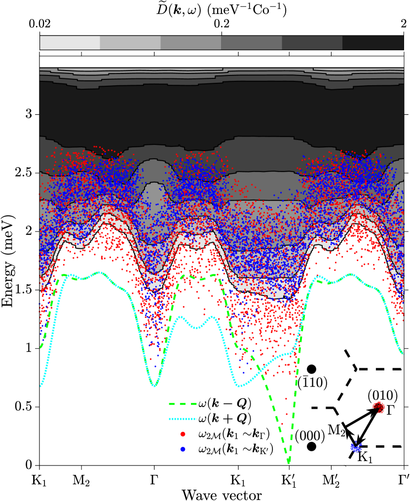
Figure 11: (Color online) Gray shaded contour plot ($\log_{10}$ scale) of the two-magnon density of states in Eq. (9) along a wave vector path equivalent to the one in Fig. 7(b). The density of states is very small (below the plotted gray range) in the region immediately above the lower continuum boundary, given by the lower energy of the curves $\omega^{-}(\bm{k})$ and $\omega^{+}(\bm{k})$, plotted by dashed green and dotted cyan lines, respectively. The dominant two-magnon states that contribute in this region have one of the magnons near the origin, with a very low density of states in energy (sparsely-distributed red dots). At higher energy, more two-magnon scattering channels become available, such as having one magnon near K (blue dots), leading to a significant increase in the density of states above the lowest black contour line. The colored dotted regions near $\Gamma$ and K₁ in the bottom-right diagram indicate the phase spaces sampled by the two-magnon events plotted as dots in the main panel.

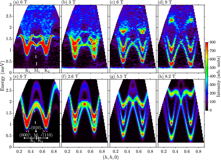
Figure 12: (Color online) INS data (top row) as a function of $c$-axis applied magnetic field, compared with the predicted spin wave spectrum (bottom row) for a sample containing equal-weight magnetic domains of types 1 and 2 in Fig. 1(c). The color is the intensity in arbitrary units and the wave vector path is $(h\mp 0.05,h\pm 0.05,\pm 0.3)$, where $\pm$ values indicate the integration ranges. Panel (a) was collected with $E_{\mathrm{i}}=3.53$ meV at 1.7 K and (b)–(d) with $E_{\mathrm{i}}=3.81$ meV at 0.1 K. (e)–(h) Corresponding spin wave spectra within LSWT using the Hamiltonian parametersIto et al. (2017) $J_{1}=1.67$ meV, $J_{z}=0.08$ meV, $g=4$ and $\Delta=0.954$, assuming no quantum renormalizations of the dispersions. For each panel, the intensity scale and magnetic field value (listed in the panel titles) were selected to give the best agreement with the data for energy scans at K₁. The quasielastic scattering below 0.2 meV has been omitted.

Close inspection of Fig. 2 shows that the continuum of scattering appears to be separated in energy from the one-magnon modes at lower energies. We propose below that the most likely explanation of this effect is a suppression of the density of states for two-particle continuum scattering, rather than a genuine energy gap between the two types of excitations. The energy separation is most apparent in the center of the figure at M${}_{2}^{\prime}$, where the highest-energy magnon is at 1.65 meV, whereas significant continuum scattering starts only above about 1.8 meV. This separation is reduced (but still present) inside the spin wave cones centered at K${}_{1,2}^{\prime}$, as significant continuum scattering does not start immediately above the sharp modes and there is a clear drop in intensity between the two scattering signals. Note that an energy separation between the two-magnon continuum and the magnon modes is also clearly visible in the spin wave model calculation in Figs. 7(b) and 9(b). This apparent separation in the calculation seems to be at odds with the fact that the magnon spectrum is gapless [as there is a Goldstone mode at the $\Gamma$ point $\omega(\bm{0})=0$ associated with rotations of the ordered spins in the $ab$ plane], so one can always create a magnon pair excitation at the wave vector and energy of a single magnon (by creating one magnon in the pair at the origin); therefore, no energy gap is expected between one-magnon states and the two-magnon continuum, as illustrated in Fig. 8(d). Indeed, close inspection of energy scans through Figs. 7(b) and 9(b) shows that no finite gap is present, the continuum intensity is just very small immediately above the one-magnon dispersions. This is because the relevant two-magnon states that contribute just above the lower boundary of the continuum are dominated by pairs where one magnon is created close to zero energy near the origin; since the dispersion there is very steep [see Fig. 7(b) solid line near $\Gamma$], the density of states in energy for such two-magnon processes is very small, leading to an apparent suppression of the two-magnon signal near the lower boundary. This is illustrated in Fig. 11, where the gray shadings separated by black lines in the top half of the graph illustrate a contour map (on a log scale) of the two-magnon density of states $\widetilde{D}(\bm{k},\omega)$ in Eq. (9). Note that the region immediately above the lower boundary onset (the lower of the dashed green and dotted cyan lines) is below the plotted gray range, indicating a very low density of states. The sparsely-distributed red dots correspond to two-magnon states where one magnon is near the origin, showing that two-magnon continuum states do exist just above the magnon dispersions. However, their density is very low compared to higher energies, for example above the lowest black contour line, where new scattering channels become available and there is a significant contribution from pair states with one magnon near the (gapped) K point (blue dots). Based on this analysis, we conclude that the apparent separation in the data between the higher-energy continuum scattering and the lower-energy sharp spin wave modes is consistent with the assumed gapless spin wave spectrum and is most likely due to a suppression of intensity towards the lower boundary of the continuum due to a reduced density of states in that region.

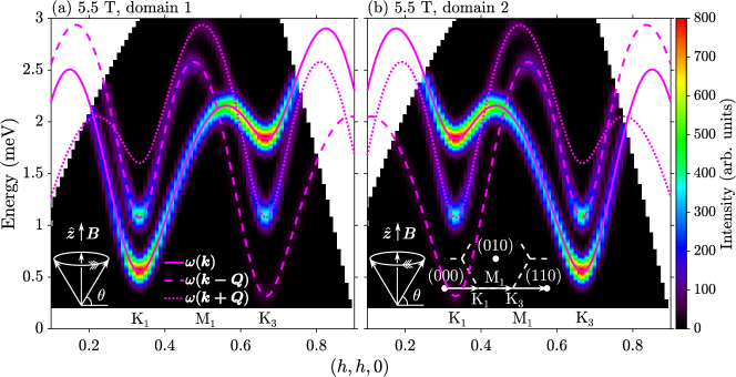
Figure 13: (Color online) Spin wave spectrum in the cone phase in a $c$-axis applied field for (a) domain 1 and (b) domain 2, to be compared with the data in Fig. 12(c). The two domains have different spectra, mirror-reversed about the zone boundary M₁ point. The color is the one-magnon cross-section from Appendix A, for the same parameters as in Fig. 12 (g). The white bottom-left inset in each panel shows the sense of rotation of the spins with respect to the applied field $\bm{B}$ (vertical arrow), as per Fig. 1(c). The $\omega(\bm{k})$, $\omega(\bm{k-Q})$ and $\omega(\bm{k+Q})$ dispersions are plotted as solid, dashed and dotted magenta lines, respectively.

IV Magnon dispersions in the cone phase in c-axis magnetic field

Here we present INS measurements of the magnetic excitations as a function of magnetic field applied along the $c$ axis, which are sensitive to the presence of multiple magnetic domains. For the Hamiltonian in Eq. (1), the mean-field ground state has ordered spins rotating by $120^{\circ}$ between NN sites in the triangular layers, with two possible senses of rotation illustrated in Fig. 1(c) left/right panel, corresponding to a counterclockwise/clockwise rotation between sites displaced along the $\bm{a}+\bm{b}$ direction (labeled ‘domain 1’/‘domain 2’), respectively. The two structures are degenerate in the absence of DM interactions, so a macroscopic sample would be expected to contain magnetic domains of both types, selected via spontaneous symmetry breaking when cooling through the magnetic ordering temperature. In zero magnetic field, the two domains have identical dispersion relations and dynamical structure factors. In a $c$-axis applied magnetic field, spins cant towards the field while their in-plane component continues to rotate in the $ab$ plane, forming a cone structure. The two domains remain degenerate in applied field, but their excitation spectrum is different, as the primary magnon dispersion $\omega(\bm{k})$ acquires an additive term [$C_{\bm{k}}$ in Eqs. (3) and (4) in Appendix A] that changes sign between the two domain types. Previous magnetization,Susuki et al. (2013) nuclear magnetic resonanceKoutroulakis et al. (2015) and ultrasound velocityQuirion et al. (2015) measurements in $c$-axis applied field have indicated that the cone phase persists up to 12 T. Here we present measurements well within this field range (up to 9 T) to test whether the sample contains both types of domains, selected via spontaneous symmetry breaking, as expected in the absence of DM interactions.

Figure 12 (top row) shows how the magnetic excitations along a representative wave vector path evolve upon increasing the applied field. In zero field [panel (a)], the spectrum has mirror symmetry around the zone boundary M₁ point with two intense, gapped spin wave modes visible, clearly separated at M₁ and nearly overlapping near the K_1,3 points, followed by continuum scattering at higher energies. In the following we focus on the sharp spin wave modes, as they contain the key information about the domain type. At 3 T [panel (b)], there are clearly three modes resolved near the K points, which separate further upon increasing field to 6, then 9 T [panels (c) and (d)], with the mirror symmetry of the spectrum around M₁ preserved throughout. The data presented have contributions from pixels at wave vectors $\bm{k}$ not only along the nominal $(110)$ scan direction, but also along other directions in the $(hk0)$ plane that are equivalent up to symmetry operations of the crystal lattice point group; this was performed for the purpose of improving the counting statistics. We have explicitly verified that slices through the raw, unsymmetrized data display all the same features.

In order to interpret the observed behavior, we compare in Fig. 13 the predicted spectrum within LSWT for magnetic domains of both types at a representative intermediate field where the mode splitting is large enough to clearly observe the key features. Panel (a) shows the spectrum for domain 1, a strong asymmetry of the spectrum is expected between the two K points, with only two modes carrying weight at each wave vector. Domain 2 would have a mirror-reversed spectrum around M₁, again with only two modes visible at a general wave vector. The behavior of a single magnetic domain of either type is clearly incompatible with the data in Fig. 12 (top row), which shows three modes at a general wave vector, with mirror symmetry of the spectrum around M₁. Assuming the sample contains coexisting, equal-weight magnetic domains of both types, the spectrum would be the sum of Figs. 13(a) and (b) plotted in Fig. 12(g), which restores the mirror symmetry around M₁ and gives three modes at a general wave vector, as in the data.

To test the two magnetic domains scenario further, we plot in Fig. 12 (bottom row) the LSWT-predicted evolution of the spectrum as a function of field. The plotted fields were selected for best agreement with the data in the panels above, for energy scans at the K₁ point. Comparison with the data shows that the key features, such as the number of visible modes, their trend as a function of field and the overall symmetry of the intensity pattern, are well reproduced, providing clear evidence that the sample contains equal-weight magnetic domains of both types, as expected in the absence of DM interactions. We attribute the remaining quantitative discrepancies between the precise experimental dispersion shapes and the model calculations, and the fact that the best agreement is obtained for fields slightly different (by about 10%) from the actual values, to quantum effects beyond the LSWT approximation, which we have already established in Sec. III.3 need to be included to quantitatively reproduce the dispersions.

V Conclusions

To summarize, we have reported extensive single-crystal high-resolution inelastic neutron scattering measurements of the spin dynamics in the pseudospin-$\frac{1}{2}$ triangular antiferromagnet Ba₃CoSb₂O₉ in the $120^{\circ}$ ordered phase. We have observed sharp, resolution-limited magnons throughout reciprocal space with no decay, but with a strongly renormalized dispersion and much reduced intensities at high energies compared to linear spin wave theory. At higher energies, we have observed a very strong continuum of magnetic scattering extending up at least $4\times$ the maximum one-magnon energy. The relatively large intensity in the continuum is much underestimated by linear spin wave theory, and only some limited low-energy features are captured qualitatively by a two-magnon cross-section, leaving unexplained a rich structure of intensity modulations in the continuum as a function of both energy and wave vector. We have proposed empirical wave vector-dependent renormalizations that parametrize quantitatively the experimental dispersion in the full three-dimensional Brillouin zone, and we have explicitly verified that magnon decays are kinematically disallowed for the observed strongly-renormalized dispersion, explaining why magnons are sharp throughout the Brillouin zone. Based on a quantitative comparison of the measured intensities with the spin wave dynamical structure factor, we have proposed that a transfer of spectral weight occurs from the high-energy magnons (whose energy is strongly renormalized downwards) to the higher-energy continuum. The experimental observation of strong dispersion renormalizations and an enhanced-intensity scattering continuum with structured intensity modulations suggests that quantum fluctuations and interaction effects are well beyond what can be captured by the spin wave approximation. Finally, through measurements of the dispersion relations in $c$-axis applied magnetic field, we have determined the presence of equal-weight magnetic domains with opposite senses for the spin rotation in the ground state, as expected in the absence of Dzyaloshinskii-Moriya interactions, when the sense of spin rotation in the 120^∘ ordered ground state is selected via spontaneous symmetry breaking.

Appendix A Dispersion relations and dynamical structure factor in linear spin wave theory

This section outlines the LSWT calculation of the dispersion relation and dynamical structure factor used in the analysis of the INS data. Based on previous electron spin resonance,Susuki et al. (2013) nuclear magnetic resonance,Koutroulakis et al. (2015) ultrasound velocityQuirion et al. (2015) and neutron diffractionMa et al. (2016) measurements of Ba₃CoSb₂O₉, we assume antiferromagnetic XXZ interactions between NN sites within the triangular layers (intralayer exchanges) and an antiferromagnetic XXZ interaction between NN sites on adjacent layers (interlayer exchange), as per Eq. (1). Figures 1(b)–(c) illustrate the exchange paths and the spin alignments in the ground state in zero applied magnetic field. Ordered spins are confined to the $ab$ plane, are antiparallel along $\bm{c}$, and rotate by $120^{\circ}$ between the three sites of every in-plane triangle. The propagation vector for the magnetic structure is $\bm{Q}=(\frac{1}{3},\frac{1}{3},1)$. The left/right panels in Fig. 1(c) show the magnetic domains with counterclockwise/clockwise rotation.

In a magnetic field applied along the $c$ axis, the Hamiltonian in Eq. (1) acquires the additional Zeeman term

$$\mathcal{H}_{\mathrm{Z}}=-g\mu_{\mathrm{B}}B\sum_{i}S_{i}^{z},$$

where $g$ is the $g$ factor and to describe the spin axes we use the Cartesian coordinate system $(x,y,z)$ with $\bm{\hat{x}}\parallel(\bm{a}+\bm{b})$ and $\bm{\hat{z}}\parallel\bm{c}$, as illustrated in Fig. 1(c) (bottom left). The magnetic structure in applied field is a cone, where the ordered spins cant out of the $xy$ plane by an angle $\theta$, with the in-plane components continuing to have the same pattern as in Fig. 1(c). The two magnetic domains with opposite sense of rotation in the $xy$ plane are degenerate throughout the cone phase. The canting angle $\theta$ is obtained from minimizing the mean-field ground state energy (per spin)

$$E_{\mathrm{MF}}=[J(\bm{Q})\cos^{2}{\theta}+\Delta{}J(\bm{0})\sin^{2}{\theta}]S^{2}-g\mu_{\mathrm{B}}BS\sin{\theta},$$

which gives

$$\sin{\theta}=\frac{g\mu_{\mathrm{B}}B}{2S[\Delta{}J(\bm{0})-J(\bm{Q})]}.$$

Here $J(\bm{k})$ is the Fourier transform of the in-plane exchange interactions, given by

$$\begin{split}J(\bm{k})=J_{1}\left[\cos{2\pi{}h}+\cos{2\pi{}k}+\cos{2\pi(h+k)}\right]+J_{z}\cos{\pi{}l}\end{split}$$

for a general wave vector $\bm{k}$ indexed as $(h,k,l)$ in reciprocal lattice units of the structural unit cell, i.e. $\bm{k}=h\bm{a}^{\ast}+k\bm{b}^{\ast}+l\bm{c}^{\ast}$. The canting angle $\theta$ increases up to the saturation field $B_{\rm{sat}}=2S[\Delta J(\bm{0})-J(\bm{Q})]/(g\mu_{\mathrm{B}})$, above which spins are entirely polarized along the field ($\theta=\pi/2$ for $B\geq B_{\rm{sat}}$).

It is convenient to perform the analytic spin wave calculations in the cone phase in a right-handed reference frame $(\xi,\eta,\zeta)$ that follows the ordered spin precession in the ground state, such that $\zeta$ is along the local ordered spin direction and $\xi$ is perpendicular to the ordered spin in the helical plane. For concreteness, we first discuss the calculation for domain 1 with counterclockwise rotation in Fig. 1(c) (left panel). In this case, the transformation from the rotating reference frame to the global ($x,y,z$) frame is obtained by first performing a rotation in the $\zeta\eta$ plane by the canting angle $\theta$, and then rotating in the $xy$ plane by the helical angle $\phi_{i}=\bm{Q}\cdot\bm{r}_{i}+\Phi$, where $\bm{r}_{i}$ is the position of the $i$th spin and $\Phi$ is the phase of the spin at the origin [$\Phi=\frac{\pi}{2}$ for both domains illustrated in Fig. 1(c)]. The transformation of the spin operators is then given by

$$S^{x}_{i} =S^{\zeta}_{i}\cos{\theta}\cos{\phi_{i}}-S^{\xi}_{i}\sin{\phi_{i}}-S^{\eta}_{i}\sin{\theta}\cos{\phi_{i}},$$

$$S^{y}_{i} =S^{\zeta}_{i}\cos{\theta}\sin{\phi_{i}}+S^{\xi}_{i}\cos{\phi_{i}}-S^{\eta}_{i}\sin{\theta}\sin{\phi_{i}},$$

$$S^{z}_{i} =S^{\zeta}_{i}\sin{\theta}+S^{\eta}_{i}\cos{\theta}.$$

The spin Hamiltonian for the NN intralayer interactions [first term of Eq. (1)] in the rotating reference frame has the form

$$\mathcal{H}_{\mathrm{NN}}= J_{1}\sum_{\langle{ij}\rangle}[(\cos^{2}{\theta}\cos{\phi_{ij}}+\Delta\sin^{2}{\theta})S^{\zeta}_{i}S^{\zeta}_{j}$$

$$+\cos{\phi_{ij}}S^{\xi}_{i}S^{\xi}_{j}+(\sin^{2}{\theta}\cos{\phi_{ij}}+\Delta\cos^{2}{\theta})S^{\eta}_{i}S^{\eta}_{j}$$

$$+\sin{\theta}\sin{\phi_{ij}}(S^{\xi}_{i}S^{\eta}_{j}-S^{\eta}_{i}S^{\xi}_{j})],$$

where $\phi_{ij}=\phi_{i}-\phi_{j}$. A similar expression describes the interlayer interactions. The advantage of working in the rotating frame is that all spins are ferromagnetically aligned and the calculation is reduced to one magnetic sublattice and a reduced hexagonal unit cell $a\times b\times(c/2)$.

Using a Holstein-Primakoff transformation,Holstein and Primakoff (1940) a Fourier transformation, and neglecting terms higher than quadratic order in the boson operators, the spin Hamiltonian in the rotating frame is obtained asVeillette et al. (2005)

$$\mathcal{H}= \frac{1}{2}\sum_{\bm{k}}\mathbf{X}^{\dagger}\mathbf{H}\mathbf{X}-Ng\mu_{\mathrm{B}}B(S+1/2)\sin{\theta}$$

$$+N[J(\bm{Q})\cos^{2}{\theta}+\Delta{}J(\bm{0})\sin^{2}{\theta}]S(S+1)$$

where the sum is over all wave vectors $\bm{k}$ in the first Brillouin zone of the reduced unit cell and $N$ is the total number of spin sites. The operator basis is chosen to be $\mathbf{X}^{\dagger}=\begin{pmatrix}\alpha_{\bm{k}}^{\dagger}&\alpha_{-\bm{k}}\end{pmatrix}$, where $\alpha_{\bm{k}}^{\dagger}$ ($\alpha_{\bm{k}}$) creates (annihilates) a plane-wave magnon. The Hamiltonian matrix then has the form

$$\mathbf{H}=\begin{pmatrix}A_{\bm{k}}+C_{\bm{k}}&B_{\bm{k}}\\ B_{\bm{k}}&A_{\bm{k}}-C_{\bm{k}}\\ \end{pmatrix},$$

where

$$A_{\bm{k}} =S(a_{\bm{k}}+b_{\bm{k}}),$$

$$B_{\bm{k}} =S(a_{\bm{k}}-b_{\bm{k}}),$$

$$C_{\bm{k}} =S\sin{\theta}\left[J(\bm{k}+\bm{Q})-J(\bm{k}-\bm{Q})\right],$$ (3)

and

$$a_{\bm{k}} =\left[\Delta{}J(\bm{k})-J(\bm{Q})\right]\cos^{2}{\theta}+b_{\bm{k}}\sin^{2}{\theta},$$

$$b_{\bm{k}} =\frac{1}{2}\left[J(\bm{k}-\bm{Q})+J(\bm{k}+\bm{Q})\right]-J(\bm{Q}).$$

Using standard methods to diagonalize the bilinear boson Hamiltonian,White et al. (1965) the dispersion relation is obtained as

$$\hbar\omega(\bm{k})=\sqrt{A_{\bm{k}}^{2}-B_{\bm{k}}^{2}}+C_{\bm{k}},$$ (4)

which by periodicity holds for a general wave vector $\bm{k}$ in reciprocal space. The one-magnon excitations are polarized transverse to the ordered spin direction $\zeta$, and the dynamical structure factors (per spin) are obtained as

$$S^{\xi\xi}(\bm{k},\omega) =\frac{Z_{\xi}{}S}{2}(u_{\bm{k}}+v_{\bm{k}})^{2}\delta[\hbar\omega-\hbar\omega(\bm{k})]$$

$$=\frac{Z_{\xi}{}S}{2}\frac{A_{\bm{k}}+B_{\bm{k}}}{\hbar\omega(\bm{k})}\delta[\hbar\omega-\hbar\omega(\bm{k})],$$ (5)

$$S^{\eta\eta}(\bm{k},\omega) =\frac{Z_{\eta}{}S}{2}(u_{\bm{k}}-v_{\bm{k}})^{2}\delta[\hbar\omega-\hbar\omega(\bm{k})]$$

$$=\frac{Z_{\eta}{}S}{2}\frac{A_{\bm{k}}-B_{\bm{k}}}{\hbar\omega(\bm{k})}\delta[\hbar\omega-\hbar\omega(\bm{k})],$$ (6)

$$S^{\xi\eta}(\bm{k},\omega) =-S^{\eta\xi}(\bm{k},\omega)=i\frac{S}{2}\delta[\hbar\omega-\hbar\omega(\bm{k})],$$ (7)

where $u_{\bm{k}}=\cosh{\Theta_{\bm{k}}}$, $v_{\bm{k}}=\sinh{\Theta_{\bm{k}}}$ and $\tanh{2\Theta_{\bm{k}}}=B_{\bm{k}}/A_{\bm{k}}$. The intensity prefactors for in-plane ($Z_{\xi}$) and out-of-plane magnons ($Z_{\eta}$) are both unity in LSWT; they are introduced here as a way to parametrize an intensity renormalization due to effects beyond the LSWT approximation.

The two-magnon (${2\mathcal{M}}$) excitations are polarized longitudinal to the spin direction, and the dynamical structure factor (per spin) is obtained as

$$\begin{split}S^{\zeta\zeta}_{2\mathcal{M}}(\bm{k},\omega)=\frac{Z_{\zeta}}{2N}\sum_{\bm{k}_{1},\bm{k}_{2}}(u_{-\bm{k}_{1}}v_{\bm{k}_{2}}+u_{\bm{k}_{2}}v_{-\bm{k}_{1}})^{2}\\ \times\delta[\hbar\omega-\hbar\omega(\bm{k}_{1})-\hbar\omega(\bm{k}_{2})]\delta(\bm{k}+\bm{k}_{1}-\bm{k}_{2}+\bm{\tau}),\end{split}$$ (8)

with the density of states (meV^-1Co^-1) for two-magnon excitations given by

$$D(\bm{k},\omega)=\frac{1}{N}\sum_{\bm{k}_{1},\bm{k}_{2}}\delta[\hbar\omega-\hbar\omega(\bm{k}_{1})-\hbar\omega(\bm{k}_{2})]\delta(\bm{k}+\bm{k}_{1}-\bm{k}_{2}+\bm{\tau}),$$

where $\bm{\tau}$ is a reciprocal lattice vector of the reduced unit cell. Similar to the expressions for the one-magnon dynamical structure factor, we introduce in Eq. (8) a two-magnon intensity prefactor $Z_{\zeta}$ to parametrize an intensity renormalization attributed to effects beyond the LSWT approximation. Following Ref. Mourigal et al., 2013, we neglect the mixed transverse-longitudinal correlations (such as $S^{\xi\zeta}$), as for the TLHAF model they have relatively negligible weight compared to the purely transverse or purely longitudinal correlations.

For a spin-$\frac{1}{2}$ system, the dynamical structure factor components are required to satisfy the sum ruleLorenzana et al. (2005)

$$\frac{1}{N}\sum_{\bm{k}}\int^{\infty}_{-\infty}d(\hbar\omega)\;S^{\alpha\alpha}(\bm{k},\omega)=\frac{1}{4},$$

where $\alpha=\xi,\eta,\zeta$ and the sum is over all wave vectors in the first Brillouin zone of the reduced unit cell. Note that the longitudinal component $S^{\zeta\zeta}$ includes two-magnon scattering $S^{\zeta\zeta}_{2\mathcal{M}}$ and elastic Bragg scattering $(S-\Delta S)^{2}$, which gives the following sum rule for the two-magnon contribution:

$$\frac{1}{N}\sum_{\bm{k}}\int^{\infty}_{-\infty}d(\hbar\omega)\;S^{\zeta\zeta}_{2\mathcal{M}}(\bm{k},\omega)=\frac{1}{4}-(S-\Delta{S})^{2},$$

where $\Delta{S}$ is the reduction in the ordered spin moment in the ground state due to zero-point spin wave fluctuations. For the Hamiltonian parameters in Table 1, $\Delta{S}=0.152$ and the above sum rules are satisfied for intensity prefactor values $Z_{\xi}=0.804$, $Z_{\eta}=0.734$ and $Z_{\zeta}=0.733$. In the fits to the experimental spin wave data, we allowed the relative intensity of in-plane to out-of-plane magnons to vary unconstrained, with the best overall agreement found for $Z_{\eta}/Z_{\xi}=0.60$, to be compared with 0.91 imposed by the sum rule constraints and 1 in LSWT. In all calculations, the two-magnon scattering intensity was scaled to the in-plane one-magnon intensity assuming both satisfy the sum rule constraints, which gives $Z_{\zeta}/Z_{\xi}=0.91$.

Rotating back to the fixed global frame, the dynamical structure factors for one-magnon ($1\mathcal{M}$) and two-magnon ($2\mathcal{M}$) excitations are as follows:

$$S^{zz}_{1\mathcal{M}}(\bm{k},\omega)= S^{\eta\eta}(\bm{k},\omega)\cos^{2}{\theta},$$

$$S^{zz}_{2\mathcal{M}}(\bm{k},\omega)= S^{\zeta\zeta}_{2\mathcal{M}}(\bm{k},\omega)\sin^{2}{\theta},$$

$$S^{xx}_{1\mathcal{M}}(\bm{k},\omega)= \frac{1}{4}[S^{\xi\xi}(\bm{k}-\bm{Q},\omega)+S^{\xi\xi}(\bm{k}+\bm{Q},\omega)]$$

$$+\frac{1}{4}\sin^{2}{\theta}[S^{\eta\eta}(\bm{k}-\bm{Q},\omega)+S^{\eta\eta}(\bm{k}+\bm{Q},\omega)]$$

$$+\frac{i}{2}\sin{\theta}[S^{\xi\eta}(\bm{k}+\bm{Q},\omega)-S^{\xi\eta}(\bm{k}-\bm{Q},\omega)],$$

$$S^{xx}_{2\mathcal{M}}(\bm{k},\omega)= \frac{1}{4}\cos^{2}{\theta}[S^{\zeta\zeta}_{2\mathcal{M}}(\bm{k}-\bm{Q},\omega)+S^{\zeta\zeta}_{2\mathcal{M}}(\bm{k}+\bm{Q},\omega)],$$

where by symmetry $S^{xx}(\bm{k},\omega)=S^{yy}(\bm{k},\omega)$. The two-magnon density of states in the global frame is obtained as

$$\widetilde{D}(\bm{k},\omega)=\frac{1}{2}\left[D(\bm{k}-\bm{Q},\omega)+D(\bm{k}+\bm{Q},\omega)\right].$$ (9)

The above analytic expressions for the dispersion relations and dynamical structure factor were checked explicitly against numerical calculations performed using spinw.Toth and Lake (2015) The interpretation of the above equations for the one-magnon dynamical structure factor is that in the global frame there are two in-plane-polarized modes $\omega(\bm{k}-\bm{Q})\equiv\omega^{-}(\bm{k})$ and $\omega(\bm{k}+\bm{Q})\equiv\omega^{+}(\bm{k})$ and one out-of-plane mode $\omega(\bm{k})$, so there are three dispersion branches for a general wave vector $\bm{k}$.

All the above expressions for the dispersion relation and dynamical structure factor are for the magnetic domain 1 in Fig. 1(c) (left panel); the results for domain 2 (right panel) are obtained by replacing $\bm{Q}$ with $-\bm{Q}$ in Eq. (3), which changes the sign of the $C_{\bm{k}}$ term in Eq. (4) with the $A_{\bm{k}}$ and $B_{\bm{k}}$ terms unchanged. This implies that in zero field when $\theta=0$ and $C_{\bm{k}}=0$, the two domains have identical dispersions and dynamical structure factors, and so cannot be distinguished experimentally. However, for finite field $B$ the $C_{\bm{k}}$ term is finite and the two domains have different primary mode dispersions. This is illustrated in Fig. 13, which shows the calculated spin wave spectrum in finite field [panels (a) and (b) for domains 1 and 2, respectively], showing that the primary magnon dispersion (magenta solid line) is different in the two cases, with soft modes at different wave vectors [K₁ in (a) and K₃ in (b)].

Finally, total neutron scattering cross-section including the neutron polarization factor is

$$I(\bm{k},\omega)= Z[n(\hbar\omega)+1]f^{2}(\lvert{\bm{k}}\rvert)$$

$$\times\sum_{\alpha}\left(1-\frac{k_{\alpha}^{2}}{\lvert{\bm{k}}\rvert^{2}}\right)S^{\alpha\alpha}(\bm{k},\omega),$$ (10)

where $Z$ is an overall intensity scale factor, $n(\hbar\omega)=1/\left(e^{\hbar\omega/k_{\mathrm{B}}T}-1\right)$ is the finite-temperature Bose factor, $f(\lvert{\bm{k}}\rvert)$ is the spherical magnetic form factor for Co²⁺ ions, and $k_{\alpha}$ denotes the $\alpha=x,y,z$ component of the wave vector transfer $\bm{k}$.

In the fits to the experimental data, we used the renormalized dispersion (see Appendix B) in place of $\hbar\omega(\bm{k})$ in the dynamical structure factor expressions in Eqs. (5)–(7). The effects of the instrumental energy resolution were included by replacing the delta functions in the same equations with a lineshape of finite energy width that could describe well the observed profile of the incoherent elastic line. For each separate instrument configuration, the appropriate energy resolution lineshape was parametrized by a main Gaussian with an additional less intense Gaussian on the low-energy side to reproduce the observed slightly-asymmetric energy lineshape. In the fits, the resolution profile was assumed constant as a function of energy transfer.

Appendix B Empirical renormalizations of the LSWT dispersion

Parameter	Value
$J_{1}$	$1.653$	meV
$J_{z}$	$0.082$	meV
$\Delta$	$0.949$
$Z_{\eta}/Z_{\xi}$	$0.60$
$\alpha_{\mathrm{M}}$	$1.434$	meV
$\beta_{\mathrm{M}}$	$0.019$	meV
$\gamma_{\mathrm{M}}$	$17.18$	meVÅ2
$\delta_{\mathrm{M}}$	$0.151$
$\kappa_{\mathrm{M}}$	$1.333$
$\alpha_{\mathrm{K/2}}$	$2.040$	meV
$\beta_{\mathrm{K/2}}$	$-0.025$	meV
$\gamma_{\mathrm{K/2}}$	$13.12$	meVÅ2
$\delta_{\mathrm{K/2}}$	$0.192$
$\kappa_{\mathrm{K/2}}$	$1^{{\dagger}}$
$\epsilon$	$0.1566^{{\dagger}}$
$Z_{\zeta}/Z_{\xi}$	$0.91^{{\dagger}}$

Table 1: Parameter values for the best fit to the observed one-magnon dispersion relations, obtained from a global fit to several selected scans through the four-dimensional INS data. In the fit the Hamiltonian parameters ($J_{1}$,$J_{z}$,$\Delta$) were constrained to reproduce the saturation magnetization field as per Eq. (2). The dagger ^† indicates parameter values kept fixed in the global fit. The table omits the overall intensity scale $Z$, the parametrization of the non-magnetic background and the instrumental energy resolution, as these vary between different measurement configurations and are discussed elsewhere. For descriptions of the listed parameters, see Appendices A and B.

In this section, we detail the empirical renormalizations applied to the analytic LSWT dispersion relation in order to fit the experimental magnon dispersion. In particular we consider the introduction of soft modes in the dispersion at the M and near K/2 points.

To introduce local minima in the dispersion, we consider the virtual mixing of the bare dispersion $\hbar\omega_{\mathrm{LSWT}}$ in Eq. (4) with fictitious gapped parabolic modes $\hbar\Omega_{i}$, centered near wave vector positions $i=$ M and K/2. This mixing can be parametrized in the basis of the two modes by a $2\times 2$ Hamiltonian matrix

$$\mathbf{H}=\begin{pmatrix}\hbar\omega_{\mathrm{LSWT}}&c_{i}\\ c_{i}&\hbar\Omega_{i}\\ \end{pmatrix},$$

where the off-diagonal coupling term is defined as $c_{i}\equiv\delta_{i}\,\hbar\omega_{\mathrm{LSWT}}$, with $\delta_{i}$ a dimensionless parameter. This form ensures the coupling $c_{i}$ is largest near the top of the dispersion and becomes negligibly small at low energies. The above Hamiltonian can then be diagonalized to obtain the eigenenergies

$$\lambda^{\pm}=\frac{\hbar\omega_{\mathrm{LSWT}}+\hbar\Omega_{i}}{2}\pm\sqrt{\left(\frac{\hbar\omega_{\mathrm{LSWT}}-\hbar\Omega_{i}}{2}\right)^{2}+c_{i}^{2}},$$

where the lower mode $\lambda^{-}$ is a smoothly-varying function that inherits a local minimum from the gapped virtual mode $\hbar\Omega_{i}$ and interpolates towards the unperturbed $\hbar\omega_{\mathrm{LSWT}}$ in the regions away from the soft mode. This is graphically illustrated in Fig. 4, compare the solid magenta line ($\lambda^{-}$) with the dashed magenta line ($\hbar\omega_{\mathrm{LSWT}}$).

The fictitious gapped modes were parametrized by the general dispersion form

$$\hbar\Omega_{i}=\alpha_{i}+\beta_{i}\cos{\pi{}l}+\gamma_{i}[(q_{x}-q_{ix})^{2}+\kappa_{i}(q_{y}-q_{iy})^{2}],$$

where the first term ($\alpha_{i}$) parametrizes the overall energy gap, the second term allows for a dispersion along the interlayer $l$ direction, and $\gamma_{i}$ is the coefficient of the in-plane quadratic dispersion. $(q_{ix},q_{iy})$ are the in-plane wave vector coordinates (in Å^-1) of the paraboloid center (minimum energy gap) in a Cartesian reference frame, where the $q_{y}$ coordinate is along the direction from the closest $\Gamma$ point to the paraboloid center and $q_{x}$ is transverse to $q_{y}$ in the $hk$ plane. $\kappa_{i}$ parametrizes the relative dispersions along the two orthogonal in-plane directions, i.e. $\kappa_{i}=1$ corresponds to an isotropic dispersion with circular constant-energy contours and $\kappa_{i}>1$ corresponds to elliptical constant-energy contours elongated along the transverse $q_{x}$ direction. Figure 3(g) shows clear oval-shaped contours around the M points, elongated along the hexagonal zone-boundary contour (dashed white line), and this elongation was parametrized in the fit by the ellipticity parameter $\kappa_{\mathrm{M}}\simeq 1.3$. For the soft modes near K/2, we found an isotropic description to be sufficient, so we fixed $\kappa_{\mathrm{K/2}}=1$ in the fit. As expected for a quasi-2D system, the fitted interlayer dispersion is almost negligible at the relatively high energies of the soft modes ($\lvert{\beta_{i}}\rvert/\alpha_{i}\simeq 0.01$ for both $i=\mathrm{M}$ and K/2).

The procedure for obtaining the renormalized magnon dispersion $\hbar\omega$ from the bare $\hbar\omega_{\mathrm{LSWT}}$ after considering the couplings with both types of virtual parabolic modes is illustrated in Fig. 4, where the lower (magenta) solid line has the desired soft modes at both types of positions with symmetric dispersions around the local minima, as seen in the experimental data. Note that the original magnon dispersion is not perfectly sinusoidal along the $\Gamma$-K line, with the maximum slightly offset from the halfway position K/2; so in order to obtain an approximately symmetric shape for the dispersion near the soft mode along the $\Gamma$-K direction, the paraboloid $\hbar\Omega_{\mathrm{K}}/2$ was centered at position $\epsilon(\bm{a}^{\ast}+\bm{b}^{\ast})$, with $\epsilon$ slightly offset (see Table 1) from the value 1/6 that corresponds to the exact K/2 wave vector position. Using the latter position would have resulted in a highly asymmetric shape of the dispersion near the upper soft mode, not compatible with the experimental data in Fig. 2.

In order to calculate the renormalized dispersion relation, it is sufficient to work in the minimal Brillouin zone sector $\Gamma$-M-K-$\Gamma$ in the $hk$ plane and $0\leq l<1$, as any general wave vector $\bm{k}$ can be remapped to this volume using reciprocal lattice translations followed by symmetry operations of the $6/mmm$ lattice point group. For wave vectors within this minimal reciprocal space volume, we calculated iteratively the mixing of $\hbar\omega_{\mathrm{LSWT}}$ with virtual paraboloids located at equivalent (up to reciprocal lattice translations or lattice point group symmetry operations) M and K/2-type positions within a large radius in the two-dimensional reciprocal space at the same $l$ value; in this way, we ensured the “final” renormalized dispersion (that is fitted to the experimental data) still satisfies all lattice point group symmetries and is numerically smooth (so there is no step change in gradient across the minimal volume boundaries). A contour map of the renormalized dispersion surface in the $(hk0)$ plane is shown in Fig. 5(b).

The Hamiltonian and dispersion renormalization parameters obtained from a best fit to the experimental data are listed in Table 1, and numerical code to generate the dispersion relation from these parameters is available from Ref. dat, .

We note that in order to capture all modulations of the full magnon dispersion surface in a transparent way that can also be easily implemented analytically, several empirical parameters have been introduced: three Hamiltonian parameters ($J_{1}$,$J_{z}$,$\Delta$), five parameters ($\alpha_{i}$, $\beta_{i}$, $\gamma_{i}$, $\delta_{i}$, $\kappa_{i}$) for each of the soft modes at M and near K/2, in addition to independent intensity scale factors for the in-plane and out-of-plane magnons. Although some parameters were kept fixed in the fit and additional constraints were imposed, this still left a very large number of degrees of freedom in the fit (over 10) and in practice many parameters were strongly correlated. Therefore, Table 1 parameter values are to be interpreted as representative values for the best level of agreement that can be obtained with the data; the meaningful result of the analysis is the final parametrized dispersion surface obtained with those parameters and its specific features, not the individual values of each of the parameters.

References

- Chubukov and Golosov (1991) A. V. Chubukov and D. I. Golosov, J. Phys. Condens. Matter 3, 69 (1991).
- Honecker (1999) A. Honecker, J. Phys. Condens. Matter 11, 4697 (1999).
- Alicea et al. (2009) J. Alicea, A. V. Chubukov, and O. A. Starykh, Phys. Rev. Lett. 102, 137201 (2009).
- Farnell et al. (2009) D. J. J. Farnell, R. Zinke, J. Schulenburg, and J. Richter, J. Phys. Condens. Matter 21, 406002 (2009).
- Zheng et al. (2006) W. Zheng, J. O. Fjærestad, R. R. P. Singh, R. H. McKenzie, and R. Coldea, Phys. Rev. B 74, 224420 (2006).
- Starykh et al. (2006) O. A. Starykh, A. V. Chubukov, and A. G. Abanov, Phys. Rev. B 74, 180403(R) (2006).
- Anderson (1973) P. Anderson, Mater. Res. Bull. 8, 153 (1973).
- Kalmeyer and Laughlin (1987) V. Kalmeyer and R. B. Laughlin, Phys. Rev. Lett. 59, 2095 (1987).
- Balents (2010) L. Balents, Nature 464, 199 (2010).
- Huse and Elser (1988) D. A. Huse and V. Elser, Phys. Rev. Lett. 60, 2531 (1988).
- Jolicoeur and Le Guillou (1989) T. Jolicoeur and J. C. Le Guillou, Phys. Rev. B 40, 2727 (1989).
- Singh and Huse (1992) R. R. P. Singh and D. A. Huse, Phys. Rev. Lett. 68, 1766 (1992).
- Bernu et al. (1994) B. Bernu, P. Lecheminant, C. Lhuillier, and L. Pierre, Phys. Rev. B 50, 10048 (1994).
- White and Chernyshev (2007) S. R. White and A. L. Chernyshev, Phys. Rev. Lett. 99, 127004 (2007).
- Chernyshev and Zhitomirsky (2009) A. L. Chernyshev and M. E. Zhitomirsky, Phys. Rev. B 79, 144416 (2009).
- Oh et al. (2013) J. Oh, M. D. Le, J. Jeong, J.-H. Lee, H. Woo, W.-Y. Song, T. G. Perring, W. J. L. Buyers, S.-W. Cheong, and J.-G. Park, Phys. Rev. Lett. 111, 257202 (2013).
- Mourigal et al. (2013) M. Mourigal, W. T. Fuhrman, A. L. Chernyshev, and M. E. Zhitomirsky, Phys. Rev. B 88, 094407 (2013).
- Verresen et al. (2019) R. Verresen, R. Moessner, and F. Pollmann, Nat. Phys. 15, 750 (2019).
- Ferrari and Becca (2019) F. Ferrari and F. Becca, Phys. Rev. X 9, 031026 (2019).
- Mezio et al. (2011) A. Mezio, C. N. Sposetti, L. O. Manuel, and A. E. Trumper, EPL (Europhysics Letters) 94, 47001 (2011).
- Ghioldi et al. (2015) E. A. Ghioldi, A. Mezio, L. O. Manuel, R. R. P. Singh, J. Oitmaa, and A. E. Trumper, Phys. Rev. B 91, 134423 (2015).
- Ghioldi et al. (2018) E. A. Ghioldi, M. G. Gonzalez, S.-S. Zhang, Y. Kamiya, L. O. Manuel, A. E. Trumper, and C. D. Batista, Phys. Rev. B 98, 184403 (2018).
- Zhang et al. (2019) S.-S. Zhang, E. A. Ghioldi, Y. Kamiya, L. O. Manuel, A. E. Trumper, and C. D. Batista, Phys. Rev. B 100, 104431 (2019).
- Momma and Izumi (2011) K. Momma and F. Izumi, J. Appl. Crystallogr. 44, 1272 (2011).
- Doi et al. (2004) Y. Doi, Y. Hinatsu, and K. Ohoyama, J. Phys. Condens. Matter 16, 8923 (2004).
- Shirata et al. (2012) Y. Shirata, H. Tanaka, A. Matsuo, and K. Kindo, Phys. Rev. Lett. 108, 057205 (2012).
- Zhou et al. (2012) H. D. Zhou, C. Xu, A. M. Hallas, H. J. Silverstein, C. R. Wiebe, I. Umegaki, J. Q. Yan, T. P. Murphy, J.-H. Park, Y. Qiu, J. R. D. Copley, J. S. Gardner, and Y. Takano, Phys. Rev. Lett. 109, 267206 (2012).
- Abragam and Pryce (1951) A. Abragam and M. H. L. Pryce, Proc. R. Soc. London. Ser. A. Math. Phys. Sci. 206, 173 (1951).
- Susuki et al. (2013) T. Susuki, N. Kurita, T. Tanaka, H. Nojiri, A. Matsuo, K. Kindo, and H. Tanaka, Phys. Rev. Lett. 110, 267201 (2013).
- Koutroulakis et al. (2015) G. Koutroulakis, T. Zhou, Y. Kamiya, J. D. Thompson, H. D. Zhou, C. D. Batista, and S. E. Brown, Phys. Rev. B 91, 024410 (2015).
- Quirion et al. (2015) G. Quirion, M. Lapointe-Major, M. Poirier, J. A. Quilliam, Z. L. Dun, and H. D. Zhou, Phys. Rev. B 92, 014414 (2015).
- Ma et al. (2016) J. Ma, Y. Kamiya, T. Hong, H. B. Cao, G. Ehlers, W. Tian, C. D. Batista, Z. L. Dun, H. D. Zhou, and M. Matsuda, Phys. Rev. Lett. 116, 087201 (2016).
- Ono et al. (2003) T. Ono, H. Tanaka, H. Aruga Katori, F. Ishikawa, H. Mitamura, and T. Goto, Phys. Rev. B 67, 104431 (2003).
- Ito et al. (2017) S. Ito, N. Kurita, H. Tanaka, S. Ohira-Kawamura, K. Nakajima, S. Itoh, K. Kuwahara, and K. Kakurai, Nat. Commun. 8, 235 (2017).
- Kamiya et al. (2018) Y. Kamiya, L. Ge, T. Hong, Y. Qiu, D. L. Quintero-Castro, Z. Lu, H. B. Cao, M. Matsuda, E. S. Choi, C. D. Batista, M. Mourigal, H. D. Zhou, and J. Ma, Nat. Commun. 9, 2666 (2018).
- Prabhakaran and Boothroyd (2017) D. Prabhakaran and A. Boothroyd, J. Cryst. Growth 468, 345 (2017).
- Bewley et al. (2011) R. I. Bewley, J. W. Taylor, and S. M. Bennington., Nucl. Instruments Methods Phys. Res. Sect. A 637, 128 (2011).
- Coldea et al. (2015) R. Coldea et al., ISIS Pulsed Neutron and Muon Source (2015), doi: 10.5286/ISIS.E.RB1510491 .
- Coldea et al. (2016) R. Coldea et al., ISIS Pulsed Neutron and Muon Source (2016), doi: 10.5286/ISIS.E.RB1610390 .
- Arnold et al. (2014) O. Arnold, J. C. Bilheux, J. M. Borreguero, A. Buts, S. I. Campbell, L. Chapon, M. Doucet, N. Draper, R. Ferraz Leal, M. A. Gigg, V. E. Lynch, A. Markvardsen, D. J. Mikkelson, R. L. Mikkelson, R. Miller, K. Palmen, P. Parker, G. Passos, T. G. Perring, P. F. Peterson, S. Ren, M. A. Reuter, A. T. Savici, J. W. Taylor, R. J. Taylor, R. Tolchenov, W. Zhou, and J. Zikovsky, Nucl. Instruments Methods Phys. Res. Sect. A Accel. Spectrometers, Detect. Assoc. Equip. 764, 156 (2014).
- Ewings et al. (2016) R. Ewings, A. Buts, M. Le, J. van Duijn, I. Bustinduy, and T. Perring, Nucl. Instruments Methods Phys. Res. Sect. A 834, 132 (2016).
- Chubukov et al. (1994) A. V. Chubukov, S. Sachdev, and T. Senthil, Journal of Physics: Condensed Matter 6, 8891 (1994).
- (43) Data archive weblink.
- Holstein and Primakoff (1940) T. Holstein and H. Primakoff, Phys. Rev. 58, 1098 (1940).
- Veillette et al. (2005) M. Y. Veillette, J. T. Chalker, and R. Coldea, Phys. Rev. B 71, 214426 (2005).
- White et al. (1965) R. M. White, M. Sparks, and I. Ortenburger, Phys. Rev. 139, A450 (1965).
- Lorenzana et al. (2005) J. Lorenzana, G. Seibold, and R. Coldea, Phys. Rev. B 72, 224511 (2005).
- Toth and Lake (2015) S. Toth and B. Lake, J. Phys. Condens. Matter 27, 166002 (2015).