Scalable Deep Generative Modeling for Sparse Graphs

Abstract

Learning graph generative models is a challenging task for deep learning and has wide applicability to a range of domains like chemistry, biology and social science. However current deep neural methods suffer from limited scalability: for a graph with $n$ nodes and $m$ edges, existing deep neural methods require $\Omega(n^{2})$ complexity by building up the adjacency matrix. On the other hand, many real world graphs are actually sparse in the sense that $m\ll n^{2}$. Based on this, we develop a novel autoregressive model, named BiGG, that utilizes this sparsity to avoid generating the full adjacency matrix, and importantly reduces the graph generation time complexity to $O((n+m)\log n)$. Furthermore, during training this autoregressive model can be parallelized with $O(\log n)$ synchronization stages, which makes it much more efficient than other autoregressive models that require $\Omega(n)$. Experiments on several benchmarks show that the proposed approach not only scales to orders of magnitude larger graphs than previously possible with deep autoregressive graph generative models, but also yields better graph generation quality.

1 Introduction

Representing a distribution over graphs provides a principled foundation for tackling many important problems in knowledge graph completion (Xiao et al., 2016), de novo drug design (Li et al., 2018; Simonovsky & Komodakis, 2018), architecture search (Xie et al., 2019) and program synthesis (Brockschmidt et al., 2018). The effectiveness of graph generative modeling usually depends on learning the distribution given a collection of relevant training graphs. However, training a generative model over graphs is usually quite difficult due to their discrete and combinatorial nature.

Classical generative models of graphs, based on random graph theory (Erdős & Rényi, 1960; Barabási & Albert, 1999; Watts & Strogatz, 1998), have been long studied but typically only capture a small set of specific graph properties, such as degree distribution. Despite their computational efficiency, these distribution models are usually too inexpressive to yield competitive results in challenging applications.

Recently, deep graph generative models that exploit the increased capacity of neural networks to learn more expressive graph distributions have been successfully applied to real-world tasks. Prominent examples include VAE-based methods (Kipf & Welling, 2016; Simonovsky & Komodakis, 2018), GAN-based methods (Bojchevski et al., 2018), flow models (Liu et al., 2019; Shi et al., 2020) and autoregressive models (Li et al., 2018; You et al., 2018; Liao et al., 2019). Despite the success of these approaches in modeling small graphs, e.g. molecules with hundreds of nodes, they are not able to scale to graphs with over 10,000 nodes.

A key shortcoming of current deep graph generative models is that they attempt to generate a full graph adjacency matrix, implying a computational cost of $\Omega(n^{2})$ for a graph with $n$ nodes and $m$ edges. For large graphs, it is impractical to sustain such a quadratic time and space complexity, which creates an inherent trade-off between expressiveness and efficiency. To balance this trade-off, most recent work has introduced various conditional independence assumptions (Liao et al., 2019), ranging from the fully auto-regressive but slow GraphRNN (You et al., 2018), to the fast but fully factorial GraphVAE (Simonovsky & Komodakis, 2018).

In this paper, we propose an alternative approach that does not commit to explicit conditional independence assumptions, but instead exploits the fact that most interesting real-world graphs are sparse, in the sense that $m\ll n^{2}$. By leveraging sparsity, we develop a new graph generative model, BiGG (BIg Graph Generation), that streamlines the generative process and avoids explicit consideration of every entry in an adjacency matrix. The approach is based on three key elements: (1) an $O(\log n)$ process for generating each edge using a binary tree data structure, inspired by R-MAT (Chakrabarti et al., 2004); (2) a tree-structured autoregressive model for generating the set of edges associated with each node; and (3) an autoregressive model defined over the sequence of nodes. By combining these elements, BiGG can generate a sparse graph in $O((n+m)\log n)$ time, which is a substantial improvement over $\Omega(n^{2})$.

For training, the design of BiGG also allows every context embedding in the autoregressive model to be computed in only $O(\log n)$ sequential steps, which enables significant gains in training speed through parallelization. By comparison, the context embedding in GraphRNN requires $O(n^{2})$ sequential steps to compute, while GRAN requires $O(n)$ steps. In addition, we develop a training mechanism that only requires sublinear memory cost, which in principle makes it possible to train models of graphs with millions of nodes on a single GPU.

On several benchmark datasets, including synthetic graphs and real-world graphs of proteins, 3D mesh and SAT instances, BiGG is able to achieve comparable or superior sample quality than the previous state-of-the-art, while being orders of magnitude more scalable.

To summarize the main contributions of this paper:

• We propose an autoregressive generative model, BiGG, that can generate sparse graphs in $O((n+m)\log n)$ time, successfully modeling graphs with 100k nodes on 1 GPU.

• The training process can be largely parallelized, requiring only $O(\log n)$ steps to synchronize learning updates.

• Memory cost is reduced to $O(\sqrt{m\log n})$ for training and $O(\log n)$ for inference.

• BiGG not only scales to orders of magnitude larger graphs than current deep models, it also yields comparable or better model quality on several benchmark datasets.

Other related work There has been a lot of work (Chakrabarti et al., 2004; Robins et al., 2007; Leskovec et al., 2010; Airoldi et al., 2009) on generating graphs with a set of specific properties like degree distribution, diameter, and eigenvalues. All these classical models are hand-engineered to model a particular family of graphs, and thus not general enough. Besides the general graphs, a lot of work also exploit domain knowledge for better performance in specific domains. Examples of this include (Kusner et al., 2017; Dai et al., 2018; Jin et al., 2018; Liu et al., 2018) for modeling molecule graphs, and (You et al., 2019) for SAT instances. See Appendix A for more discussions.

2 Model

A graph $G=(V,E)$ is defined by a set of nodes $V$ and set of edges $E\subseteq V\times V$, where a tuple $e_{i}=(u,v)\in E$ is used to represent an edge between node $u$ and $v$. We denote $n=|V|$ and $m=|E|$ as the number of nodes and edges in $G$ respectively. Note that a given graph may have multiple equivalent adjacency matrix representations, with different node orderings. However, given an ordering of the nodes $\pi$, there is a one-to-one mapping between the graph structure $G$ and the adjacency matrix $A^{\pi}\in\{0,1\}^{n\times n}$.

Our goal is to learn a generative model, $p(G)$, given a set of training graphs $\mathcal{D}_{train}=\left\{G_{1},G_{2},\ldots,G_{|\mathcal{D}_{train}|}\right\}$. In this paper, we assume the graphs are not attributed, and focus on the graph topology only. Such an assumption implies

$$p\left(G\right) =p(V)p(E|V)=p(|V|=n)\sum_{\pi}p(E,\pi|n)$$

$$=p(|V|=n)\sum_{\pi}p(A^{\pi}),$$ (1)

where $p(E,\pi|n)$ is the probability of generating the set of edges $E$ under a particular ordering $\pi$, which is equivalent to the probability of a particular adjacency matrix $A^{\pi}$. Here, $p(|V|=n)$ is the distribution of number of nodes in a graph. In this paper, we use a single canonical ordering $\pi(G)$ to model each graph $G$, as in (Li et al., 2018):

$$p(G)\simeq p(|V|=n)p(A^{\pi(G)}),$$ (2)

which is clearly a lower bound on $p(G)$ (Liao et al., 2019). We estimate $p(|V|=n)$ directly using the empirical distribution over graph size, and only learn an expressive model for $p(A)$. In the following presentation, we therefore omit the ordering $\pi$ and assume a default canonical ordering of nodes in the graph when appropriate.

As $A$ will be extremely sparse for large sparse graphs ($m\ll n^{2}$), generating only the non-zero entries in $A$, i.e., the edge set $E$, will be much more efficient than the full matrix:

$$p(A)=p(e_{1})p(e_{2}|e_{1})\ldots p(e_{m}|e_{1},\ldots,e_{m-1}),$$ (3)

where each $e_{i}=(u,v)$ include the indices of the two nodes associated with one edge, resulting in a generation process of $m$ steps. We order the edges following the node ordering, hence this process generates all the edges for the first row in $A$, before generating the second row, etc. A naive approach to generating a single edge will be $O(n)$ if we factorize $p(e_{i})=p(u)p(v|u)$ and assume both $p(u)$ and $p(v|u)$ to be simple multinomials over $n$ nodes. This, however, will not give us any benefit over traditional methods.

2.1 Recursive edge generation

The main scalability bottleneck is the large output space. One way to reduce the output space size is to use a hierarchical recursive decomposition, inspired by the classic random graph model R-MAT (Chakrabarti et al., 2004). In R-MAT, each edge is put into the adjacency matrix by dividing the 2D matrix into 4 equally sized quadrants, and recursively descending into one of the quadrants, until reaching a single entry of the matrix. In this generation process, the complexity of generating each edge is only $O(\log n)$.

Figure 1: Recursive generation of the edge $e=(u,v)$ given $u$.

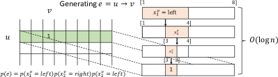
We adopt the recursive decomposition design of R-MAT, and further simplify and neuralize it, to make our model efficient and expressive. In our model, we generate edges following the node ordering row by row, so that each edge only needs to be put into the right place in a single row, reducing the process to 1D, as illustrated in Figure 1. For any edge $(u,v)$, the process of picking node $v$ as one of $u$’s neighbors starts by dividing the node index interval $[1,n]$ in half, then recursively descending into one half until reaching a single entry. Each $v$ corresponds to a unique sequence of decisions $x^{v}_{1},...,x^{v}_{d}$, where $x^{v}_{i}\in\{\text{left},\text{right}\}$ is the $i$-th decision in the sequence, and $d=\lceil\log_{2}n\rceil$ is the maximum number of required decisions to specify $v$.

The probability of $p(v|u)$ can then be formulated as

$$\textstyle p(v|u)=\prod_{i=1}^{\lceil\log_{2}n\rceil}p(x_{i}=x^{v}_{i}),$$ (4)

where each $p(x_{i}=x^{v}_{i})$ is the probability of following the decision that leads to $v$ at step $i$.

Let us use $E_{u}=\left\{(u,v)\in E\right\}$ to denote the set of edges incident to node $u$, and $\mathcal{N}_{u}=\{v|(u,v)\in E_{u}\}$. Generating only a single edge is similar to hierarchical softmax (Mnih & Hinton, 2009), and applying the above procedure repeatedly can generate all of $|\mathcal{N}_{u}|$ edges in $O(|\mathcal{N}_{u}|\log n)$ time. But we can do better than that when generating all these edges.

Further improvement using binary trees. As illustrated in the left half of Figure 2, the process of jointly generating all of $E_{u}$ is equivalent to building up a binary tree ${\mathcal{T}}_{u}$, where each tree node $t\in{\mathcal{T}}_{u}$ corresponds to a graph node index interval $[v_{l},v_{r}]$, and for each $v\in\mathcal{N}_{u}$ the process starts from the root $[1,n]$ and ends in a leaf $[v,v]$.

Taking this perspective, we propose a more efficient generation process for $E_{u}$, which generates the tree directly instead of repeatedly generating each leaf through a path from the root. We propose a recursive process that builds up the tree following a depth-first or in-order traversal order, where we start at the root, and recursively for each tree node $t$: (1) decide if $t$ has a left child denoted as $\text{lch}(t)$, and (2) if so recurse into $\text{lch}(t)$ and generate the left sub-tree, and then (3) decide if $t$ has a right child denoted as $\text{rch}(t)$, (4) if so recurse into $\text{rch}(t)$ and generate the right sub-tree, and (5) return to $t$’s parent. This process is shown in Algorithm 1, which will be elaborated in next section.

Overloading the notation a bit, we use $p(\text{lch}(t))$ to denote the probability that tree node $t$ has a left child, when $\text{lch}(t)\neq\emptyset$, or does not have a left child, when $\text{lch}(t)=\emptyset$, under our model, and similarly define $p(\text{rch}(t))$. Then the probability of generating $E_{u}$ or equivalently tree ${\mathcal{T}}_{u}$ is

$$p(E_{u})=p({\mathcal{T}}_{u})=\prod_{t\in{\mathcal{T}}_{u}}p(\text{lch}(t))p(\text{rch}(t)).$$ (5)

This new process generates each tree node exactly once, hence the time complexity is proportional to the tree size $O(|{\mathcal{T}}_{u}|)$, and it is clear that $|{\mathcal{T}}_{u}|\leq|\mathcal{N}_{u}|\log n$, since $|\mathcal{N}_{u}|$ is the number of leaf nodes in the tree and $\log n$ is the max depth of the tree. The time saving comes from removing the duplicated effort near the root of the tree. When $|\mathcal{N}_{u}|$ is large, i.e. as some fraction of $n$ when $u$ is one of the “hub” nodes in the graph, the tree ${\mathcal{T}}_{u}$ becomes dense and our new generation process will be significantly faster, as the time complexity becomes close to $O(n)$ while generating each leaf from the root would require $\Omega(n\log n)$ time.

In the following, we present our approach to make this model fully autoregressive, i.e. making $p(\text{lch}(t))$ and $p(\text{rch}(t))$ depend on all the decisions made so far in the process of generating the graph, and make this model neuralized so that all the probability values in the model come from expressive deep neural networks.

2.2 Autoregressive conditioning for generating ${\mathcal{T}}_{u}$

1:  function recursive($u,t,h_{u}^{top}(t)$) 

2:     if is_leaf(t) then

3:        Return $\vec{1},\left\{\text{edge index that $t$ represents}\right\}$

4:     end if

5:     has_left $\sim p(\text{lch}_{u}(t)|h_{u}^{top}(t))$ using Eq. (8)

6:     if has_left then

7:        Create $lch_{u}(t)$ , and let $h_{u}^{bot}(\text{lch}_{u}(t)),\mathcal{N}_{u}^{l,t}\leftarrow$ recursive($u,\text{lch}_{u}(t),h_{u}^{top}(lch_{u}(t))$)

8:     else

9:        $h_{u}^{bot}(\text{lch}_{u}(t))\leftarrow\vec{0},\mathcal{N}_{u}^{l,t}=\emptyset$

10:     end if

11:     has_right $\sim p(\text{rch}_{u}(t)|\hat{h}_{u}^{top}(rch_{u}(t)))$ using Eq. (9)

12:     if has_right then

13:        Create $rch_{u}(t)$, and let $h_{u}^{bot}(\text{rch}_{u}(t)),\mathcal{N}_{u}^{r,t}\leftarrow$ recursive($u,\text{rch}_{u}(t),h_{u}^{top}(rch_{u}(t)))$)

14:     else

15:        $h_{u}^{bot}(\text{ rch}_{u}(t))\leftarrow\vec{0},\mathcal{N}_{u}^{r,t}=\emptyset$

16:     end if

17:     $h_{u}^{bot}(t)=\text{TreeCell}^{bot}(h_{u}^{bot}(\text{lch}_{u}(t)),h_{u}^{bot}(\text{rch}_{u}(t)))$

18:     $\mathcal{N}_{u}^{t}=\mathcal{N}_{u}^{l,t}\cup\mathcal{N}_{u}^{r,t}$

19:     Return $h_{u}^{bot}(t)$, $\mathcal{N}_{u}^{t}$

20:  end function

Algorithm 1 Generating outgoing edges of node $u$

In this section we consider how to add autoregressive conditioning to $p(\text{lch}(t))$ and $p(\text{rch}(t))$ when generating ${\mathcal{T}}_{u}$.

Figure 2: Autoregressive generation of edge-binary tree of node $u$. To generate the red node $t$, the two embeddings that captures $t$’s left subtree (orange region) and nodes with in-order traversal before $t$ (blue region) respectively are used for conditioning.

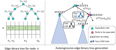
In our generation process, the decision about whether $\text{lch}(t)$ exists for a particular tree node $t$ is made after $t$, all its ancestors, and all the left sub-trees of the ancestors are generated. We can use a top-down context vector $h^{top}_{u}(t)$ to summarize all these contexts, and modify $p(\text{lch}(t))$ to $p(\text{lch}(t)|h^{top}_{u}(t))$. Similarly, the decision about $\text{rch}(t)$ is made after generating $\text{lch}(t)$ and its dependencies, and $t$’s entire left-subtree (see Figure 2 right half for illustration). We therefore need both the top-down context $h^{top}_{u}(t)$, as well as the bottom-up context $h^{bot}_{u}(\text{lch}(t))$ that summarizes the sub-tree rooted at $\text{lch}(t)$, if any. The autoregressive model for $p({\mathcal{T}}_{u})$ therefore becomes

$$p({\mathcal{T}}_{u})=\prod_{t\in{\mathcal{T}}_{u}} p(\text{lch}(t)|h^{top}_{u}(t))$$

$$p(\text{rch}(t)|h^{top}_{u}(t),h^{bot}_{u}(\text{lch}(t))),$$ (6)

and we can recursively define

$$h^{bot}_{u}(t)= \text{TreeCell}^{bot}(h^{bot}_{u}(\text{lch}(t)),h^{bot}_{u}(\text{rch}(t)))$$

$$h^{top}_{u}(\text{lch}(t))= \text{LSTMCell}(h^{top}_{u}(t),\text{embed}(\text{left}))$$ (7)

$$\hat{h}^{top}_{u}(\text{rch}(t))= \text{TreeCell}^{top}(h^{bot}_{u}(\text{lch}(t)),h^{top}_{u}(\text{lch}(t)))$$

$$h^{top}_{u}(\text{rch}(t))= \text{LSTMCell}(\hat{h}^{top}_{u}(\text{rch}(t)),\text{embed}(\text{right})),$$

where $\text{TreeCell}^{bot}$ and $\text{TreeCell}^{top}$ are two TreeLSTM cells (Tai et al., 2015) that combine information from the incoming nodes into a single node state, and $\text{embed}(\text{left})$ and $\text{embed}(\text{right})$ represents the embedding vector for the binary values “left” and “right”. We initialize $h^{bot}_{u}(\emptyset)=\vec{0}$, and discuss $h^{top}_{u}(\text{root})$ in the next section.

The distributions can then be parameterized as

$$p(\text{lch}(t)|\cdot) =\text{Bernoulli}(\sigma(W_{l}^{\top}h^{top}_{u}(t)+b_{l})),$$ (8)

$$p(\text{rch}(t)|\cdot) =\text{Bernoulli}(\sigma(W_{r}^{\top}\hat{h}^{top}_{u}(\text{rch}(t))+b_{r})).$$ (9)

2.3 Full autoregressive model

With the efficient recursive edge generation and autoregressive conditioning presented in Section 2.1 and Section 2.2 respectively, we are ready to present the full autoregressive model for generating the entire adjacency matrix $A$.

The full model will utilize the autoregressive model for $\mathcal{N}_{u}$ as building blocks. Specifically, we are going to generate the adjacency matrix $A$ row by row:

$$p(A)=p(\left\{\mathcal{N}_{u}\right\}_{u\in V})=\prod_{u\in V}p\left(\mathcal{N}_{u}|\left\{\mathcal{N}_{u^{\prime}}:u^{\prime}<u\right\}\right).$$ (10)

Let $g_{u}^{0}=h_{u}^{bot}(t_{1})$ be the embedding that summarizes ${\mathcal{T}}_{u}$, suppose we have an efficient mechanism to encode $\left[g_{1},g_{2},\ldots,g_{u}\right]$ into $h^{row}_{u}$, then we can effectively use $h^{row}_{u-1}$ to generate ${\mathcal{T}}_{u}$ and thus the entire process would become autoregressive. Again, since there are $n$ rows in total, using a chain structured LSTM would make the history length too long for large graphs. Therefore, we use an approach inspired by the Fenwick tree (Fenwick, 1994) which is a data structure that maintains the prefix sum efficiently. Given an array of numbers, the Fenwick tree allows calculating any prefix sum or updating any single entry in $O(\log L)$ for a sequence of length $L$. We build such a tree to maintain and update the prefix embeddings. We denote it as row-binary forest as such data structure is a forest of binary trees.

Figure 3: Autoregressive conditioning across rows of adjacency matrix. Embedding $h^{row}_{u-1}$ summarizes all the rows before $u$, and is used for generating ${\mathcal{T}}_{u}$ next.

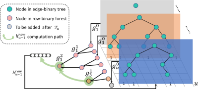
Figure 3 demonstrates one solution. Before generating the edge-binary tree ${\mathcal{T}}_{u}$, the embeddings that summarize each individual edge-binary tree $\mathcal{R}_{u}=\left\{{\mathcal{T}}_{u^{\prime}}:u^{\prime}<u\right\}$ will be organized into the row-binary forest $\mathcal{G}_{u}$. This forest is organized into $\left\lfloor\log(u-1)\right\rfloor+1$ levels, with the bottom $0$-th level as edge-binary tree embeddings. Let $g^{i}_{j}\in\mathcal{G}_{u}$ be the $j$-th node in the $i$-th level, then

$$g_{j}^{i}=\text{TreeCell}^{row}(g_{j*2-1}^{i-1},g_{j*2}^{i-1}),$$ (11)

where $0\leq i\leq\left\lfloor\log(u-1)\right\rfloor+1,1\leq j\leq\left\lfloor\frac{|\mathcal{R}_{u}|}{2^{i}}\right\rfloor$.

Embedding row-binary forest One way to embed this row-binary forest is to embed the root of each tree in this forest. As there will be at most one root in each level (otherwise the two trees in the same level will be merged into a larger tree for the next level), the number of tree roots will also be $O(\log n)$ at most. Thus we calculate $h^{row}_{u}$ as follows:

$$h^{row}_{u}=\text{LSTM}\left(\left[g^{i}_{\left\lfloor\frac{u}{2^{i}}\right\rfloor},\text{ where }u\text{ $\&$ }2^{i}=2^{i}\right]\right).$$ (12)

Here, $\&$ is the bit-level ‘and’ operator. Intuitively as in Fenwick tree, the calculation of any prefix sum of length $L$ requires the block sums that corresponds to each binary digit in the binary bits representation of integer $L$. Recall the operator $h^{top}_{u}(\cdot)$ defined in Section 2.2, here $h^{top}_{u}(root)=h^{row}_{u-1}$ when $u>1$, and equals to zero when $u=1$. With the embedding of $\mathcal{G}_{u}$ at each state served as ‘glue’, we can connect all the individual row generation modules in an autoregressive way.

Updating row-binary forest It is also efficient to update such forest every time a new $g_{u}^{0}$ is obtained after the generation of ${\mathcal{T}}_{u}$. Such an updating procedure is similar to the Fenwick tree update. As each level of this forest has at most one root node, merging in the way defined in (11) will happen at most once per each level, which effectively makes the updating cost to be $O(\log n)$.

1:  function update_forest($u,\mathcal{G}_{u-1},g_{u}^{0}$) 

2:     $\mathcal{G}_{u}=\mathcal{G}_{u-1}\cup\left\{g_{u}^{0}\right\}$

3:     for $i\leftarrow 0$ to $\left\lfloor\log(u-1)\right\rfloor$ do

4:        $j\leftarrow\arg\max_{j}\mathbb{I}\left[g^{i}_{j}\in\mathcal{G}_{u}\right]$

5:        if such $j$ exists and $j$ is an even number then

6:           $g^{i+1}_{j/2}\leftarrow\text{TreeCell}^{row}(g^{i}_{j-1},g^{i}_{j})$

7:           $\mathcal{G}_{u}\leftarrow\mathcal{G}_{u}\cup g^{i+1}_{j/2}$

8:        end if

9:     end for

10:     Update $h_{u}^{row}$ using Eq (12)

11:     Return: $h_{u}^{row},\mathcal{G}_{u}$, $\mathcal{R}_{u-1}\cup\left\{g_{u}^{0}\right\}$

12:  end function

12:  

13:  Input: The number of nodes $n$

14:  $h_{0}^{row}\leftarrow\vec{0},\mathcal{R}_{0}=\emptyset,\mathcal{G}_{0}=\emptyset,E=\emptyset$

15:  for $u\leftarrow 1$ to $n$ do

16:     Let $t_{1}$ be the root of an empty edge-binary tree

17:     $g_{u}^{0},\mathcal{N}_{u}\leftarrow$ recursive$(u,t_{1},h_{u-1}^{row})$

18:     $h_{u}^{row},\mathcal{G}_{u},\mathcal{R}_{u}\leftarrow$ update_forest($u,\mathcal{R}_{u-1},\mathcal{G}_{u-1},g_{u}^{0}$)

19:  end for

20:  Return: $G$ with $V=\left\{1,\ldots,n\right\}$ and $E=\cup_{u=1}^{n}\mathcal{N}_{u}$

Algorithm 2 Generating graph using BiGG

Algorithm 2 summarizes the entire procedure for sampling a graph from our model in a fully autoregressive manner.

Theorem 1

BiGG generates a graph with $n$ node and $m$ edges in $O\left((n+m)\log n\right)$ time. In the extreme case where $m\simeq n^{2}$, the overall complexity becomes $O(n^{2})$.

Proof  The generation of each edge-binary tree in Section 2.2 requires time complexity proportional to the number of nodes in the tree. The Fenwick tree query and update both take $O(\log n)$ time, hence maintaining the data structure takes $O(n\log n)$. The overall complexity is $O\left(n\log n+\sum_{u=1}^{n}|{\mathcal{T}}_{u}|\right)$. For a sparse graph $|{\mathcal{T}}_{u}|=O(|\mathcal{N}_{u}|\log n)$, hence $\sum_{u=1}^{n}|{\mathcal{T}}_{u}|=\sum_{u=1}^{n}|\mathcal{N}_{u}|\log n=O(m\log n)$. For a complete graph, where $m=O(n^{2})$, each ${\mathcal{T}}_{u}$ will be a full binary tree with $n$ leaves, hence $|{\mathcal{T}}_{u}|=2n-1$ and the overall complexity would be $O(n\log n+n^{2})=O(n^{2})$.  

3 Optimization

In this section, we propose several ways to scale up the training of our auto-regressive model. For simplicity, we focus on how to speed up the training with a single graph. Training multiple graphs can be easily extended.

3.1 Training with $O(\log n)$ synchronizations

A classical autoregressive model like LSTM is fully sequential, which allows no concurrency across steps. Thus training LSTM with a sequence of length $L$ takes $\Omega(L)$ of synchronized computation. In this section, we show how to exploit the characteristic of BiGG to increase concurrency during training.

Figure 4: Parallelizing computation during training. The four stages are executed sequentially. In each stage, the embeddings of nodes with the same color can be computed concurrently.

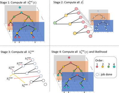
Given a graph $G$, estimating the likelihood under the current model can be divided into four steps.

1. Computing $h_{u}^{bot}(t),\forall u\in V,t\in{\mathcal{T}}_{u}$ : as the graph is given during training, the corresponding edge-binary trees $\left\{{\mathcal{T}}_{u}\right\}$ are also known. From Eq (7) we can see that the embeddings $h_{u}^{bot}(t)$ of all nodes at the same depth of tree can be computed concurrently without dependence, and the synchronization only happens between different depths. Thus $O(\log n)$ steps of synchronization is sufficient.

2. Computing $g_{j}^{i}\in\mathcal{G}_{n}$: the row-binary forest grows monotonically, thus the forest $\mathcal{G}_{n}$ in the end contains all the embeddings needed for computing $\left\{h_{u}^{row}\right\}$. Similarly, computing $\left\{g_{j}^{i}\right\}$ synchronizes $O(\log n)$ steps.

3. Computing $h_{u}^{row},\forall u\in V$: as each $h_{u}^{row}$ runs an LSTM independently, this stage simply runs LSTM on a batch of $n$ sequences with length $O(\log n)$.

4. Computing $h_{u}^{top}$ and likelihood: the last step computes the likelihood using Eq (8) and  (9). This is similar to the first step, except that the computation happens in a top-down direction in each ${\mathcal{T}}_{u}$.

Figure 4 demonstrates this process. In summary, the four stages each take $O(\log n)$ steps of synchronization. This allows us to train large graphs much more efficiently than a simple sequential autoregressive model.

3.2 Model parallelism

It is possible that during training the graph is too large to fit into memory. Thus to train on large graphs, model parallelism is more important than data parallelism.

To split the model, as well as intermediate computations, into different machines, we divide the adjacency matrix into multiple consecutive chunks of rows, where each machine is responsible for one chunk. It is easy to see that by doing so, Stage 1 and Stage 4 mentioned in Section 3.1 can be executed concurrently on all the machines without any synchronization, as the edge-binary trees can be processed independently once the conditioning states like $\left\{h_{u}^{row}\right\}$ are made ready by synchronization.

Figure 5: Model parallelism for training single graph. Red circled nodes are computed on GPU 1 but is required by GPU 2 as well.

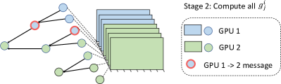
Figure 5 illustrates the situation when training a graph with 7 nodes using 2 GPUs. During Stage 1, GPU 1 and 2 work concurrently to compute $\left\{g_{u}^{0}\right\}_{u=1}^{3}$ and $\left\{g_{u}^{0}\right\}_{u=4}^{7}$, respectively. In Stage 2, the embeddings $g_{1}^{1}$ and $g_{3}^{0}$ are needed by GPU 2 when computing $g_{1}^{2}$ and $g_{2}^{1}$. We denote such embeddings as ‘g-messages’. Note that such ‘g-messages’ will transit in the opposite direction when doing a backward pass in the gradient calculation. Passing ‘g-messages’ introduces serial dependency across GPUs. However as the number of such embeddings is upper bounded by $O(\log n)$ depth of row-binary forest, the communication cost is manageable.

3.3 Reducing memory consumption

Sublinear memory cost: Another way to handle the memory issue when training large graphs is to recompute certain portions of the hidden layers in the neural network when performing backpropagation, to avoid storing such layers during the forward pass. Chen et al. (2016) introduces a computation scheduling mechanism for sequential structured neural networks that achieves $O(\sqrt{L})$ memory growth for an $L$-layer neural network.

We divide rows as in Section 3.2. During the forward pass, only the ‘g-messages’ between chunks are kept. The only difference from the previous section is that the edge-binary tree embeddings are recomputed, due to the single GPU limitation. The memory cost will be:

$$O(\max\left\{k\log n,\frac{m}{k}\right\})$$ (13)

Here $O(k\log n)$ accounts for the memory holding the ‘g-message’, and $O(\frac{m}{k})$ accounts for the memory of ${\mathcal{T}}_{u}$ in each chunk. The optimal $k$ is achieved when $k\log n=\frac{m}{k}$, hence $k=O(\sqrt{\frac{m}{\log n}})$ and the corresponding memory cost is $O(\sqrt{m\log n})$. Also note that such sublinear cost requires only one additional feedforward in Stage 1, so this will not hurt much of the training speed.

Bits compression: The vector $h_{u}^{bot}(t)$ summarizes the edge-binary tree structure rooted at node $t$ for $u$-th row in adjacency matrix $A$, as defined in Eq (7). As node $t$ represents the interval $[v_{l},v_{r}]$ of the row, another equivalent way is to directly use $A[u,v_{l}:v_{r}]$, i.e., the binary vector to represent $h_{u}^{bot}(t)$. Each $h_{u}^{bot}(t^{\prime})$ where $t^{\prime}=[v^{\prime}_{l},v^{\prime}_{r}]\subset t=[v_{l},v_{r}]$ is also a binary vector. Thus no neural network computation is needed in the subtree rooted at node $t$. Suppose we use such bits representation for any nodes that have the corresponding interval length no larger than $L$, then for a full edge-binary tree ${\mathcal{T}}_{u}$ (i.e., $u$ connects to every other node in graph) which has $2n-1$ nodes in the tree, the corresponding storage required for neural part is $\lceil 2\frac{n}{L}-1\rceil$ which essentially reduces the memory consumption of neural network to $\frac{1}{L}$ of the original cost. Empirically we use $L=256$ in all experiments, which saves $50\%$ of the memory during training without losing any information in representation.

Note that to represent an interval $A[u,v_{l}:v_{r}]$ of length $b=v_{r}-v_{l}+1\leq L$, we use vector $\mathbf{v}\in\left\{-1,0,1\right\}^{L}$ where

$$\mathbf{v}=\left[\underbrace{-1,\ldots,-1}_{L-b},\underbrace{A[u,v_{l}],A[u,v_{l}+1],\ldots,A[u,v_{r}]}_{b}\right]$$

That is to say, we use ternary bit vector to encode both the interval length and the binary adjacency information.

3.4 Position encoding:

During generation of $\left\{{\mathcal{T}}_{u}\right\}$, each tree node $t$ of the edge-binary tree knows the span $[v_{l},v_{r}]$ which corresponds to the columns it will cover. One way is to augment $h^{top}_{u}(t)$ with the position encoding as:

$$\hat{h}^{top}_{u}(t)=h^{top}_{u}(t)+\text{PE}(v_{r}-v_{l})$$ (14)

where PE is the position encoding using sine and cosine functions of different frequencies as in Vaswani et al. (2017). Similarly, the $h_{u}^{row}$ in Eq (12) can be augmented by $\text{PE}(n-u)$ in a similar way. With such augmentation, the model will know more context into the future, and thus help improve the generative quality.

Please refer to our released open source code located at https://github.com/google-research/google-research/tree/master/bigg for more implementation and experimental details.

4 Experiment

4.1 Model Quality Evaluation on Benchmark Datasets

In this part, we compare the quality of our model with previous work on a set of benchmark datasets. We present results on median sized general graphs with number of nodes ranging in 0.1k to 5k in Section 4.1.1, and on large SAT graphs with up to 20k nodes in Section 4.1.2. In Section 4.3 we perform ablation studies of BiGG with different sparsity and node orders.

4.1.1 General graphs

Datasets		Methods
		Erdos-Renyi	GraphVAE	GraphRNN-S	GraphRNN	GRAN	BiGG
Grid	Deg.	0.79	7.07$e^{-2}$	0.13	1.12$e^{-2}$	8.23$e^{-4}$	$\mathbf{4.12e^{-4}}$
	Clus.	2.00	7.33$e^{-2}$	3.73$e^{-2}$	7.73$e^{-5}$	3.79$e^{-3}$	$\mathbf{7.25e^{-5}}$
$|V|_{max}=361$, $|V|_{avg}\approx 210$	Orbit	1.08	0.12	0.18	1.03$e^{-3}$	1.59$e^{-3}$	$\mathbf{5.10e^{-4}}$
$|E|_{max}=684$, $|E|_{avg}\approx 392$	Spec.	0.68	1.44$e^{-2}$	0.19	1.18$e^{-2}$	1.62$e^{-2}$	$\mathbf{9.28e^{-3}}$
Protein	Deg.	5.64$e^{-2}$	0.48	4.02$e^{-2}$	1.06$e^{-2}$	1.98$e^{-3}$	$\mathbf{9.51e^{-4}}$
	Clus.	1.00	7.14$e^{-2}$	4.79$e^{-2}$	0.14	4.86$e^{-2}$	$\mathbf{2.55e^{-2}}$
$|V|_{max}=500$, $|V|_{avg}\approx 1575$	Orbit	1.54	0.74	0.23	0.88	0.13	$\mathbf{2.26e^{-2}}$
$|E|_{max}=258$, $|E|_{avg}\approx 646$	Spec.	9.13$e^{-2}$	0.11	0.21	1.88$e^{-2}$	5.13$e^{-3}$	$\mathbf{4.51e^{-3}}$
3D Point Cloud	Deg.	0.31	OOM	OOM	OOM	1.75$e^{-2}$	$\mathbf{2.56e^{-3}}$
	Clus.	1.22	OOM	OOM	OOM	0.51	0.21
$|V|_{max}=5037$, $|V|_{avg}\approx 1377$	Orbit	1.27	OOM	OOM	OOM	0.21	$\mathbf{7.18e^{-3}}$
$|E|_{max}=10886$, $|E|_{avg}\approx 3074$	Spec.	4.26$e^{-2}$	OOM	OOM	OOM	7.45$e^{-3}$	$\mathbf{3.40e^{-3}}$
Lobster	Deg.	0.24	2.09$e^{-2}$	3.48$e^{-3}$	9.26$e^{-5}$	3.73$e^{-2}$	$\mathbf{2.94e^{-5}}$
	Clus.	3.82$e^{-2}$	7.97$e^{-2}$	4.30$e^{-2}$	0.00	0.00	0.00
$|V|_{max}=100$, $|V|_{avg}\approx 53$	Orbit	2.42$e^{-2}$	1.43$e^{-2}$	2.48$e^{-4}$	2.19$e^{-5}$	7.67$e^{-4}$	$\mathbf{1.51e^{-5}}$
$|E|_{max}=99$, $|E|_{avg}\approx 52$	Spec.	0.33	3.94$e^{-2}$	6.72$e^{-2}$	1.14$e^{-2}$	2.71$e^{-2}$	$\mathbf{8.57e^{-3}}$
	Err.	1.00	0.91	1.00	0.00	0.12	0.00

Table 1: Performance on benchmark datasets. The MMD metrics uses test functions from $\left\{\text{Deg., Clus., Orbit., Spec.}\right\}$. For all the metrics, the smaller the better. Baseline results are obtained from Liao et al. (2019), where OOM indicates the out-of-memory issue.

The general graph benchmark is obtained from Liao et al. (2019) and part of it was also used in (You et al., 2018). This benchmark has four different datasets: (1) Grid, 100 2D grid graphs; (2) Protein, 918 protein graphs (Dobson & Doig, 2003); (3) Point cloud, 3D point clouds of 41 household objects (Neumann et al., 2013); (4) Lobster, 100 random Lobster graphs (Golomb, 1996), which are trees where each node is at most 2 hops away from a backbone path. Table 1 contains some statistics about each of these datasets. We use the same protocol as Liao et al. (2019) that splits the graphs into training and test sets.

Baselines: We compare with deep generative models including GraphVAE (Simonovsky & Komodakis, 2018), GraphRNN, GraphRNN-S (You et al., 2018) and GRAN  (Liao et al., 2019). We also include the Erdős–Rényi random graph model that only estimates the edge density. Since our setups are exactly the same, the baseline results are directly copied from Liao et al. (2019).

Evaluation: We use exactly the same evaluation metric as Liao et al. (2019), which compares the distance between the distribution of held-out test graphs and the generated graphs. We use maximum mean discrepancy (MMD) with four different test functions, namely the node degree, clustering coefficient, orbit count and the spectra of the graphs from the eigenvalues of the normalized graph Laplacian. Besides the four MMD metrics, we also use the error rate for Lobster dataset. This error rate reflects the fraction of generated graphs that doesn’t have Lobster graph property.

Results: Table 1 reports the results on all the four datasets. We can see the proposed BiGG outperforms all other methods on all the metrics. The gain becomes more significant on the largest dataset, i.e., the 3D point cloud. While GraphVAE and GraphRNN gets out of memory, the orbit metric of BiGG is 2 magnitudes better than GRAN. This dataset reflects the scalability issue of existing deep generative models. Also from the Lobster graphs we can see, although GRAN scales better than GraphRNN, it yields worse quality due to its approximation of edge generation with mixture of conditional independent distributions. Our BiGG improves the scalability while also maintaining the expressiveness.

4.1.2 SAT graphs

Method	VIG		VCG			LCG
	Clustering	Modularity	Variable $\alpha_{v}$	Clause $\alpha_{v}$	Modularity	Modularity
Training-24	0.53 $\pm$ 0.08	0.61 $\pm$ 0.13	5.30 $\pm$ 3.79	5.14 $\pm$ 3.13	0.76 $\pm$ 0.08	0.70 $\pm$ 0.07
G2SAT	0.41 $\pm$ 0.18 (23%)	0.55 $\pm$ 0.18 (10%)	5.30 $\pm$ 3.79 (0%)	7.22 $\pm$ 6.38 (40%)	0.71 $\pm$ 0.12 (7%)	0.68 $\pm$ 0.06 (3%)
BiGG-0.1	0.49 $\pm$ 0.21 (8%)	0.36 $\pm$ 0.21 (41%)	5.30 $\pm$ 3.79 (0%)	3.76 $\pm$ 1.21 (27%)	0.58 $\pm$ 0.16 (24%)	0.58 $\pm$ 0.11 (17%)
BiGG-0.01	0.54 $\pm$ 0.13(2%)	0.53 $\pm$ 0.21 (13%)	5.30 $\pm$ 3.79(0%)	4.28 $\pm$ 1.50 (17%)	0.71 $\pm$ 0.13 (7%)	0.67 $\pm$ 0.09 (4%)

Table 2: Training and generated graph statistics with 24 SAT formulas used in You et al. (2019). The neural baselines in Table 1 are not applicable due to scalability issue. We report mean and std of different test statistics, as well as the gap between true SAT instances.

Figure 6: Inference time per graph.

Figure 7: Training time per update.

Figure 8: Training memory cost.

In addition to comparing with general graph generative models, in this section we compare against several models that are designated for generating the Boolean Satisfiability (SAT) instances. A SAT instance can be represented using bipartite graph, i.e., the literal-clause graph (LCG). For a SAT instance with $n_{x}$ variables and $n_{c}$ clauses, it creates $n_{x}$ positive and negative literals, respectively. The canonical node ordering assigns 1 to $2*n_{x}$ for literals and $2*n_{x}+1$ to $2*n_{x}+n_{c}$ for clauses.

The following experiment largely follows G2SAT (You et al., 2019). We use the train/test split of SAT instances obtained from G2SAT website. This result in 24 and 8 training/test SAT instances, respectively. The size of the SAT graphs ranges from 491 to 21869 nodes. Note that the original paper reports results using 10 small training instances instead. For completeness, we also include such results in Appendix B.3 together with other baselines from You et al. (2019).

Baseline: We mainly compare the learned model with G2SAT, a specialized deep graph generative model for bipartite SAT graphs. Since BiGG is general purposed, to guarantee the generated adjacency matrix $A$ is bipartite, we let our model to generate the upper off-diagonal block of the adjacency matrix only, i.e., $A[0:2*n_{x},2*n_{x}:2*n_{x}+n_{c}]$.

G2SAT requires additional ‘template graph’ as input when generating the graph. Such template graph is equivalent to specify the node degree of literals in LCG. We can also enforce the degree of each node $|\mathcal{N}_{v}|$ in our model.

Evaluation: Following G2SAT, we report the mean and standard deviation of statistics with respect to different test functions. These include the modularity, average clustering coefficient and the scale-free structure parameters for different graph representations of SAT instances. Please refer to Newman (2001, 2006); Ansótegui et al. (2009); Clauset et al. (2009) for more details. In general, the closer the statistical estimation the better it is.

Results: Following You et al. (2019), we compare the statistics of graphs with the training instances in Table 2. To mimic G2SAT which picks the best action among sampled options each step, we perform $\epsilon$-sampling variant (which is denoted BiGG-$\epsilon$). Such model has $\epsilon$ probability to sample from Bernoulli distribution (as in Eq (8) (9)) each step, and $1-\epsilon$ to pick best option otherwise. This is used to demonstrate the capacity of the model. We can see that the proposed BiGG can mostly recover the statistics of training graph instances. This implies that despite being general, the full autoregressive model is capable of modeling complicated graph generative process. We additionally report the statistics of generated SAT instances against the test set in  Appendix B.3, where G2SAT outperforms BiGG in 4/6 metrics. As G2SAT is specially designed for bipartite graphs, the inductive bias it introduces allows the extrapolation to large graphs. Our BiGG is general purposed and has higher capacity, thus also overfit to the small training set more easily.

4.2 Scalability of BiGG

In this section, we will evaluate the scalability of BiGG regarding the time complexity, memory consumption and the quality of generated graphs with respect to the number of nodes in graphs.

4.2.1 Runtime and memory cost

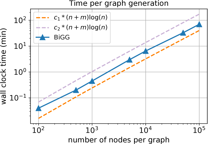
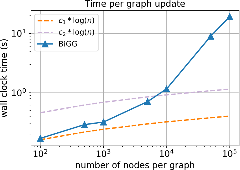
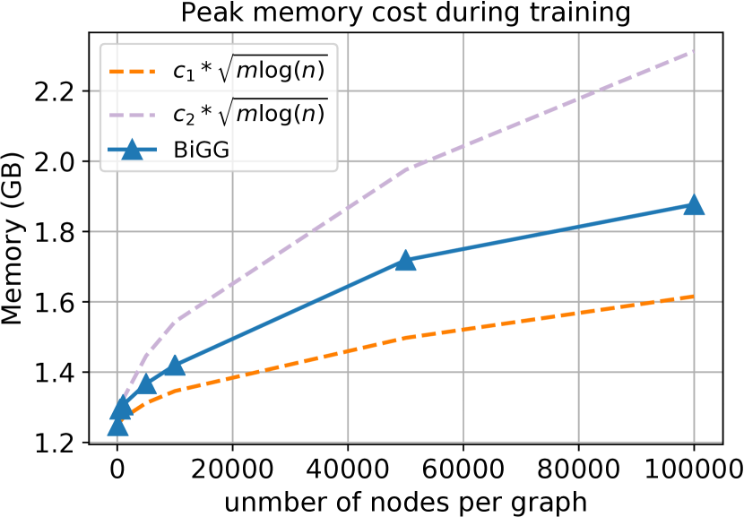
Here we empirically verify the time and memory complexity analyzed in Section 2. We run BiGG on grid graphs with different numbers of nodes $n$ that are chosen from $\left\{100,500,1k,5k,10k,50k,100k\right\}$. In this case $m=\Theta(n)$. Additionally, we also plot curves from the theoretical analysis for verification. Specifically, suppose the asymptotic cost function is $f(n,m)$ w.r.t. graph size, then if there exist constants $c_{1},c_{2},n^{\prime},m^{\prime}$ such that $c_{1}g(n,m)<f(n,m)<c_{2}g(n,m),\forall n>n^{\prime},m>m^{\prime}$, then we can claim $f(n,m)=\Theta(g(n,m))$. In Figure 8 to 8, the two constants $c_{1},c_{2}$ are tuned for better visualization.

Figure 8 reports the time needed to sample a single graph from the learned model. We can see the computation cost aligns well with the ideal curve of $O((n+m)\log n)$.

To evaluate the training time cost, we report the time needed for each round of model update, which consists of forward, backward pass of neural network, together with the update of parameters. As analyzed in Section 3.1, if there is a device with infinite FLOPS, then the time cost would be $O(\log n)$. We can see from Figure 8 that this analysis is consistent when graph size is less than 5,000. However as graph gets larger, the computation time grows linearly on a single GPU due to the limit of FLOPS and RAM.

Finally Figure 8 shows the peak memory cost during training on a single graph. We select the optimal number of chunks $k^{*}=O(\sqrt{\frac{m}{\log n}})$ as suggested in Section 3.3, and thus the peak memory grows as $O(\sqrt{m\log n})$. We can see such sublinear growth of memory can scale beyond sparse graphs with 100k of nodes.

4.2.2 Quality w.r.t graph size

	0.5k	1k	5k	10k	50k	100k
Erdős–Rényi	0.84	0.86	0.91	0.93	0.95	0.95
GRAN	$2.95e^{-3}$	$1.18e^{-2}$	0.39	1.06	N/A	N/A
BiGG	$\mathbf{3.47e^{-4}}$	$\mathbf{7.94e^{-5}}$	$\mathbf{1.57e^{-6}}$	$\mathbf{6.39e^{-6}}$	$\mathbf{6.06e^{-4}}$	$\mathbf{2.54e^{-2}}$

Table 3: MMD using orbit test function on grid graphs with different average number of nodes. N/A denotes runtime error during training, due to RAM or file I/O limitations.

In addition to the time and memory cost, we are also interested in the generated graph quality as it gets larger. To do so, we follow the experiment protocols in Section 4.1.1 on a set of grid graph datasets. The datasets have the average number of nodes ranging in $\left\{0.5k,1k,5k,10k,50k,100k\right\}$. We train on $80$ of the instances, and evaluate results on $20$ held-out instances. As calculating spectra is no longer feasible for large graphs, we report MMD with orbit test function in Table 3. For neural generative models we compare against GRAN as it is the most scalable one currently. GRAN fails on training graphs beyond 50k nodes as runtime error occurs due to RAM or file I/O limitations. We can see the proposed BiGG still preserves high quality up to grid graphs with 100k nodes. With the latest advances of GPUs, we believe BiGG would scale further due to its superior asymptomatic complexity over existing methods.

4.3 Ablation study

In this section, we take a deeper look at the performance of BiGG with different node ordering in Section 4.3.1. We also show the effect of edge density to the generative performance in Section 4.3.2.

4.3.1 BiGG with different node ordering

In the previous sections we use DFS or BFS orders. We find these two orders give consistently good performance over a variety of datasets. For the completeness, we also present results with other node orderings.

We use different orders presented in GRAN’s Github implementation. We use the protein dataset with spectral-MMD as evaluation metric. See Table 4 for the experimental results. In summary: 1) BFS/DFS give our model consistently good performance over all tasks, as it reduces the tree-width for BiGG (similar to Fig5 in GraphRNN) and we suggest to use BFS or DFS by default; 2) BiGG is also flexible enough to take any order, which allows for future research on deciding the best ordering.

DFS	BFS	Default	Kcore	Acc	Desc
3.64$e^{-3}$	3.89$e^{-3}$	4.81$e^{-3}$	2.60$e^{-2}$	3.93$e^{-3}$	4.54$e^{-3}$

Table 4: BiGG with nodes ordered by DFS, BFS, default, k-core ordering, degree accent ordering and degree descent ordering respectively on protein data. We report spectral-MMD metric here.

Determining the optimal ordering is NP-hard, and learning a good ordering is also difficult, as shown in the prior works. In this paper, we choose a single canonical ordering among graphs, as Li et al. (2018) shows that canonical ordering mostly outperforms variable orders in their Table 2, 3, while Liao et al. (2019) uses single DFS ordering (see their Sec 4.4 or github) for all experiments.

4.3.2 Performance on random graphs with decreasing sparsity

We here present experiments on Erdos-Renyi graphs with on average 500 nodes and different densities. We report spectral MMD metrics for GRAN, GT and BiGG, where GT is the ground truth Erdos-Renyi model for the data.

	1%	2%	5%	10%
GRAN	3.50$e^{-1}$	1.23$e^{-1}$	7.81$e^{-2}$	1.31$e^{-2}$
GT	9.97$e^{-4}$	4.55 $e^{-4}$	2.82$e^{-4}$	1.94$e^{-4}$
BiGG	9.47$e^{-4}$	5.08$e^{-4}$	3.18$e^{-4}$	8.38$e^{-4}$

Table 5: Graph generation quality with decreasing sparsity. We use spectral-MMD as evaluation metric against held-out test graphs.

Our main focus is on sparse graphs that are more common in the real world, and for which our approach can gain significant speed ups over the alternatives. Nevertheless, as shown in Table 5, we can see that BiGG is consistently doing much better than GRAN while being close to the ground truth across different edge densities.

5 Conclusion

We presented BiGG, a scalable autoregressive generative model for general graphs. It takes $O((n+m)\log n)$ complexity for sparse graphs, which substantially improves previous $\Omega(n^{2})$ algorithms. We also proposed both time and memory efficient parallel training method that enables comparable or better quality on benchmark and large random graphs. Future work include scaling up it further while also modeling attributed graphs.

Appendix A Detailed discussion of related work

Traditional graph generative models

There has been a lot of work (Erdös & Rényi, 1959; Barabási & Albert, 1999; Albert & lászló Barabási, 2002; Chakrabarti et al., 2004; Robins et al., 2007; Leskovec et al., 2010; Airoldi et al., 2009) on generating graphs with a set of specific properties like degree distribution, diameter, and eigenvalues. While some of them (Erdös & Rényi, 1959; Barabási & Albert, 1999; Albert & lászló Barabási, 2002; Chakrabarti et al., 2004) focused on the statistical mechanics of random and complex networks, (Robins et al., 2007) proposed exponential random graph models, known as $p\ast$ model, in estimating network models comes from the area of social sciences, statistics and social network analysis. However the $p\ast$ model usually focuses on local structural features of networks. (Airoldi et al., 2009; Leskovec et al., 2010), on the other hand, model the structure of the network as a whole by combining a global model of dense patches of connectivity with a local model.

Most of these classical models are hand-engineered to model a particular family of graphs, and thus do not have the capacity to directly learn the generative model from observed data.

Deep graph generative models

Recent work on deep neural network based graph generative models are typically much more expressive than classic random graph models, at a higher computation cost.

Similar to visual data, there are VAE (Kingma & Welling, 2013) and GAN (Goodfellow et al., 2014) based graph generative models, like GraphVAEs (Kipf & Welling, 2016; Simonovsky & Komodakis, 2018) and NetGAN (Bojchevski et al., 2018). These models typically generates large parts (or all) of the adjacency matrix independently, making them unable to model complex graph structures.

Auto-regressive models, on the other hand, generate a graph sequentially part by part, gaining expressivity but are typically more expensive as large graphs require large numbers of generation steps. Scalability is a constant important topic in this line of work, starting from (Li et al., 2018). More recent work GraphRNN (You et al., 2018) and GRAN (Liao et al., 2019) reported improved scalability and success generating graphs of up to 5,000 nodes. Our novel BiGG model advances this line of work by significantly improving both on model quality and scalability.

Besides models for general graphs, a lot of work also exploit domain knowledge for better performance in specific domains. Examples of this include (Kusner et al., 2017; Dai et al., 2018; Jin et al., 2018; Liu et al., 2018) for modeling molecule graphs, and (You et al., 2019) for SAT instances.

Appendix B More experiment details

Manual Batching

Though theoretically Section 3.1 enables the parallelism, the commonly used packages like PyTorch and TensorFlow has limited support for auto-batching operators. Also optimizing over a computation graph with $O(m)$ operators directly would be infeasible. Inspired by previous works (Looks et al., 2017; Neubig et al., 2017; Bradbury & Fu, 2018), we enable the parallelism by performing gathering and dispatching for tree or LSTM cells. This requires a single call of gemm on CUDA, instead of multiple gemv calls for the cell operations. The indices used for gathering and dispatching are computed in a customized c++ op for the sake of speed.

Parameter sharing

As the maximum depth in BiGG is $O(\log n)$, it is feasible to have different parameters per different layers for tree or LSTM cells. However experimentally it didn’t affect the performance significantly. With this change, not all parameters are updated at each step, as the trees have different heights and some are updated more often than others, which could potentially make the learning harder. Also it would make the model $O(\log n)$ times larger, and limits the potential of generating graphs larger than seen during training. So we still share the parameters of cells like other autoregressive models.

B.1 BiGG setup

Hyperparameters: For the proposed BiGG, we use embedding size $d=256$ together with position encoding for state representation. Learning rate is initialized to $1e^{-3}$ and decays to $1e^{-5}$ when training loss gets plateau.

All the experiments for both baselines and BiGG are carried out on a single V100 GPU. For the sublinear memory technique mentioned in Section 3.3, we choose $k$ (i.e., the number of blocks) as small as possible such that the training would be able to fit in a single V100 GPU. This is to make the training feasible while minimizing the synchronization overhead. Empirically the block size used in sublinear memory technique is set to 6,000 for sparse graphs.

B.2 Baselines setup

We include all the baseline numbers from their original papers when applicable, as the most experimental protocols are the same. We run the following baselines when the corresponding numbers are not reported in the literature:

• Erdős–Rényi: for the results in Table 3, we estimate the graph edge density using the training grid graphs, and generate new Erdős–Rényi random graphs with this density and compare with the held-out test graphs;

• GraphRNN-S (You et al., 2018): the result on Lobster random graphs in Table 1 is obtained by training the GraphRNN using official code  for 3000 epochs;

• GRAN (Liao et al., 2019): the results of GRAN in Table 3 are obtained by training GRAN with grid graph configuration for 8,000 epochs or 3 days, whichever limit the model reaches first.

• G2SAT (You et al., 2019): For results in Table 2 and  Table 7, we run the code  for 1000 epochs. For the test graph comparison in Table 7, we use the 8 test graphs as ‘template-graphs’ for G2SAT to generate graphs.

Method	VIG		VIG			LCG
	Clustering	Modularity	Variable $\alpha_{v}$	Clause $\alpha_{v}$	Modularity	Modularity
Training	0.50 $\pm$ 0.07	0.58 $\pm$ 0.09	3.57 $\pm$ 1.08	4.53 $\pm$ 1.09	0.74 $\pm$ 0.06	0.67 $\pm$ 0.05
CA	0.33 $\pm$ 0.08 (34%)	0.48 $\pm$ 0.10 (17%)	6.30 $\pm$ 1.53 (76%)	N/A	0.65 $\pm$ 0.08 (12%)	0.53 $\pm$ 0.05 (16%)
PS(T=0)	0.82 $\pm$ 0.04 (64%)	0.72 $\pm$ 0.13 (24%)	3.25 $\pm$ 0.89 (9%)	4.70 $\pm$ 1.59 (4%)	0.86 $\pm$ 0.05 (16%)	0.64 $\pm$ 0.05 (2%)
PS(T=1.5)	0.30 $\pm$ 0.10 (40%)	0.14 $\pm$ 0.03 (76%)	4.19 $\pm$ 1.10 (17%)	6.86 $\pm$ 1.65 (51%)	0.40 $\pm$ 0.05 (46%)	0.41 $\pm$ 0.05 (35%)
G2SAT	0.41 $\pm$ 0.09 (18%)	0.54 $\pm$ 0.11 (7%)	3.57 $\pm$ 1.08 (0%)	4.79 $\pm$ 2.80 (6%)	0.68 $\pm$ 0.07 (8%)	0.67 $\pm$ 0.03 (6%)
BiGG	0.50 $\pm$ 0.07 (0%)	0.58 $\pm$ 0.09 (0%)	3.57 $\pm$ 1.08 (0%)	4.53 $\pm$ 1.09 (0%)	0.73 $\pm$ 0.06 (1%)	0.61 $\pm$ 0.09 (9%)
BiGG-0.1	0.50 $\pm$ 0.07 (0%)	0.58 $\pm$ 0.09 (0%)	3.57 $\pm$ 1.08 (0%)	4.53 $\pm$ 1.09 (0%)	0.74 $\pm$ 0.06 (0%)	0.65 $\pm$ 0.07 (7%)

Table 6: Training and generated graph statistics with 10 SAT formulas used in You et al. (2019). Baselines results are directly copied from You et al. (2019).

Method	VIG		VIG			LCG
	Clustering	Modularity	Variable $\alpha_{v}$	Clause $\alpha_{v}$	Modularity	Modularity
Test-8	0.50 $\pm$ 0.05	0.68 $\pm$ 0.19	4.66 $\pm$ 1.92	6.33 $\pm$ 3.23	0.84 $\pm$ 0.02	0.75 $\pm$ 0.05
G2SAT	0.22 $\pm$ 0.10 (56%)	0.74 $\pm$ 0.11 (9%)	4.66 $\pm$ 1.92 (0%)	6.60 $\pm$ 4.15 (5%)	0.80 $\pm$ 0.09 (5%)	0.68 $\pm$ 0.04 (9%)
BiGG	0.37 $\pm$ 0.19 (26%)	0.28 $\pm$ 0.12 (58%)	4.66 $\pm$ 1.92 (0%)	2.74 $\pm$ 0.37 (57%)	0.44 $\pm$ 0.07 (48%)	0.48 $\pm$ 0.09 (36%)

Table 7: Test and generated graph statistics with 8 SAT formulas from https://github.com/JiaxuanYou/G2SAT. G2SAT and BiGG are trained on 24 sat formulas as in Table 2

B.3 More experimental results on SAT graphs

In main paper we reported the results on 24 training instances with the evaluation metric used in You et al. (2019). Here we include the results on the subset which is used in the original G2SAT paper (You et al., 2019). This subset contains 10 instances, with 82 to 1122 variables and 327 to 4555 clauses. This result in graphs with 6,799 nodes at most. Table 6 summarizes the results, together with other baseline results that are copied from You et al. (2019). We can see our model can almost perfectly recover the training statistics if the generative process is biased more towards high probability region (i.e., BiGG-0.1 which has 90% chance to use greedy decoding at each step). This again demonstrate that our model is flexible enough to capture complicated distributions of graph structures. On the other hand, as Table 7 shows, the G2SAT beats BiGG on 4 out of 6 metrics. Since G2SAT is a specialized generative model for bipartite graphs, it enjoys more of inductive bias towards this specific problem, and thus would work better in the low-data and extrapolation scenario. Our general purposed model thus would be expected to require more training data due to its high capacity in model space.

References

- Airoldi et al. (2009) Airoldi, E. M., Blei, D. M., Fienberg, S. E., and Xing, E. P. Mixed membership stochastic blockmodels. In Advances in Neural Information Processing Systems 21, pp. 33–40, 2009.
- Albert & lászló Barabási (2002) Albert, R. and lászló Barabási, A. Statistical mechanics of complex networks. Rev. Mod. Phys, 2002.
- Ansótegui et al. (2009) Ansótegui, C., Bonet, M. L., and Levy, J. On the structure of industrial sat instances. In International Conference on Principles and Practice of Constraint Programming, pp. 127–141. Springer, 2009.
- Barabási & Albert (1999) Barabási, A.-L. and Albert, R. Emergence of scaling in random networks. science, 286(5439):509–512, 1999.
- Bojchevski et al. (2018) Bojchevski, A., Shchur, O., Zügner, D., and Günnemann, S. Netgan: Generating graphs via random walks. arXiv preprint arXiv:1803.00816, 2018.
- Bradbury & Fu (2018) Bradbury, J. and Fu, C. Automatic batching as a compiler pass in pytorch. In Workshop on Systems for ML, 2018.
- Brockschmidt et al. (2018) Brockschmidt, M., Allamanis, M., Gaunt, A. L., and Polozov, O. Generative code modeling with graphs. arXiv preprint arXiv:1805.08490, 2018.
- Chakrabarti et al. (2004) Chakrabarti, D., Zhan, Y., and Faloutsos, C. R-mat: A recursive model for graph mining. In Proceedings of the 2004 SIAM International Conference on Data Mining, pp. 442–446. SIAM, 2004.
- Chen et al. (2016) Chen, T., Xu, B., Zhang, C., and Guestrin, C. Training deep nets with sublinear memory cost. arXiv preprint arXiv:1604.06174, 2016.
- Clauset et al. (2009) Clauset, A., Shalizi, C. R., and Newman, M. E. Power-law distributions in empirical data. SIAM review, 51(4):661–703, 2009.
- Dai et al. (2018) Dai, H., Tian, Y., Dai, B., Skiena, S., and Song, L. Syntax-directed variational autoencoder for structured data. arXiv preprint arXiv:1802.08786, 2018.
- Dobson & Doig (2003) Dobson, P. D. and Doig, A. J. Distinguishing enzyme structures from non-enzymes without alignments. Journal of molecular biology, 330(4):771–783, 2003.
- Erdös & Rényi (1959) Erdös, P. and Rényi, A. On random graphs i. Publicationes Mathematicae Debrecen, 6:290–297, 1959.
- Erdős & Rényi (1960) Erdős, P. and Rényi, A. On the evolution of random graphs. Publ. Math. Inst. Hung. Acad. Sci, 5(1):17–60, 1960.
- Fenwick (1994) Fenwick, P. M. A new data structure for cumulative frequency tables. Software: Practice and experience, 24(3):327–336, 1994.
- Golomb (1996) Golomb, S. W. Polyominoes: puzzles, patterns, problems, and packings, volume 16. Princeton University Press, 1996.
- Goodfellow et al. (2014) Goodfellow, I., Pouget-Abadie, J., Mirza, M., Xu, B., Warde-Farley, D., Ozair, S., Courville, A., and Bengio, Y. Generative adversarial nets. In Advances in neural information processing systems, pp. 2672–2680, 2014.
- Jin et al. (2018) Jin, W., Barzilay, R., and Jaakkola, T. Junction tree variational autoencoder for molecular graph generation. arXiv preprint arXiv:1802.04364, 2018.
- Kingma & Welling (2013) Kingma, D. P. and Welling, M. Auto-encoding variational bayes. arXiv preprint arXiv:1312.6114, 2013.
- Kipf & Welling (2016) Kipf, T. N. and Welling, M. Variational graph auto-encoders. arXiv preprint arXiv:1611.07308, 2016.
- Kusner et al. (2017) Kusner, M. J., Paige, B., and Hernández-Lobato, J. M. Grammar variational autoencoder. In Proceedings of the 34th International Conference on Machine Learning-Volume 70, pp. 1945–1954. JMLR. org, 2017.
- Leskovec et al. (2010) Leskovec, J., Chakrabarti, D., Kleinberg, J., Faloutsos, C., and Ghahramani, Z. Kronecker graphs: An approach to modeling networks. The Journal of Machine Learning Research, 11:985–1042, 2010.
- Li et al. (2018) Li, Y., Vinyals, O., Dyer, C., Pascanu, R., and Battaglia, P. Learning deep generative models of graphs. arXiv preprint arXiv:1803.03324, 2018.
- Liao et al. (2019) Liao, R., Li, Y., Song, Y., Wang, S., Hamilton, W., Duvenaud, D. K., Urtasun, R., and Zemel, R. Efficient graph generation with graph recurrent attention networks. In Advances in Neural Information Processing Systems, pp. 4257–4267, 2019.
- Liu et al. (2019) Liu, J., Kumar, A., Ba, J., Kiros, J., and Swersky, K. Graph normalizing flows. In Advances in Neural Information Processing Systems, pp. 13556–13566, 2019.
- Liu et al. (2018) Liu, Q., Allamanis, M., Brockschmidt, M., and Gaunt, A. Constrained graph variational autoencoders for molecule design. In Advances in Neural Information Processing Systems, pp. 7795–7804, 2018.
- Looks et al. (2017) Looks, M., Herreshoff, M., Hutchins, D., and Norvig, P. Deep learning with dynamic computation graphs. arXiv preprint arXiv:1702.02181, 2017.
- Mnih & Hinton (2009) Mnih, A. and Hinton, G. E. A scalable hierarchical distributed language model. In Advances in neural information processing systems, pp. 1081–1088, 2009.
- Neubig et al. (2017) Neubig, G., Goldberg, Y., and Dyer, C. On-the-fly operation batching in dynamic computation graphs. In Advances in Neural Information Processing Systems, pp. 3971–3981, 2017.
- Neumann et al. (2013) Neumann, M., Moreno, P., Antanas, L., Garnett, R., and Kersting, K. Graph kernels for object category prediction in task-dependent robot grasping. In Online Proceedings of the Eleventh Workshop on Mining and Learning with Graphs, pp. 0–6, 2013.
- Newman (2001) Newman, M. E. Clustering and preferential attachment in growing networks. Physical review E, 64(2):025102, 2001.
- Newman (2006) Newman, M. E. Modularity and community structure in networks. Proceedings of the national academy of sciences, 103(23):8577–8582, 2006.
- Robins et al. (2007) Robins, G., Pattison, P., Kalish, Y., and Lusher, D. An introduction to exponential random graph (p*) models for social networks. Social Networks, 29(2):173–191, 2007.
- Shi et al. (2020) Shi, C., Xu, M., Zhu, Z., Zhang, W., Zhang, M., and Tang, J. Graphaf: a flow-based autoregressive model for molecular graph generation. arXiv preprint arXiv:2001.09382, 2020.
- Simonovsky & Komodakis (2018) Simonovsky, M. and Komodakis, N. Graphvae: Towards generation of small graphs using variational autoencoders. In International Conference on Artificial Neural Networks, pp. 412–422. Springer, 2018.
- Tai et al. (2015) Tai, K. S., Socher, R., and Manning, C. D. Improved semantic representations from tree-structured long short-term memory networks. arXiv preprint arXiv:1503.00075, 2015.
- Vaswani et al. (2017) Vaswani, A., Shazeer, N., Parmar, N., Uszkoreit, J., Jones, L., Gomez, A. N., Kaiser, Ł., and Polosukhin, I. Attention is all you need. In Advances in neural information processing systems, pp. 5998–6008, 2017.
- Watts & Strogatz (1998) Watts, D. J. and Strogatz, S. H. Collective dynamics of ‘small-world’networks. nature, 393(6684):440, 1998.
- Xiao et al. (2016) Xiao, H., Huang, M., and Zhu, X. Transg: A generative model for knowledge graph embedding. In Proceedings of the 54th Annual Meeting of the Association for Computational Linguistics (Volume 1: Long Papers), pp. 2316–2325, 2016.
- Xie et al. (2019) Xie, S., Kirillov, A., Girshick, R., and He, K. Exploring randomly wired neural networks for image recognition. In Proceedings of the IEEE International Conference on Computer Vision, pp. 1284–1293, 2019.
- You et al. (2018) You, J., Ying, R., Ren, X., Hamilton, W. L., and Leskovec, J. Graphrnn: Generating realistic graphs with deep auto-regressive models. arXiv preprint arXiv:1802.08773, 2018.
- You et al. (2019) You, J., Wu, H., Barrett, C., Ramanujan, R., and Leskovec, J. G2sat: Learning to generate sat formulas. In Advances in Neural Information Processing Systems, pp. 10552–10563, 2019.