Many-Class Few-Shot Learning on Multi-Granularity Class Hierarchy

Abstract

We study many-class few-shot (MCFS) problem in both supervised learning and meta-learning settings. Compared to the well-studied many-class many-shot and few-class few-shot problems, the MCFS problem commonly occurs in practical applications but has been rarely studied in previous literature. It brings new challenges of distinguishing between many classes given only a few training samples per class. In this paper, we leverage the class hierarchy as a prior knowledge to train a coarse-to-fine classifier that can produce accurate predictions for MCFS problem in both settings. The propose model, “memory-augmented hierarchical-classification network (MahiNet)”, performs coarse-to-fine classification where each coarse class can cover multiple fine classes. Since it is challenging to directly distinguish a variety of fine classes given few-shot data per class, MahiNet starts from learning a classifier over coarse-classes with more training data whose labels are much cheaper to obtain. The coarse classifier reduces the searching range over the fine classes and thus alleviates the challenges from “many classes”. On architecture, MahiNet firstly deploys a convolutional neural network (CNN) to extract features. It then integrates a memory-augmented attention module and a multi-layer perceptron (MLP) together to produce the probabilities over coarse and fine classes. While the MLP extends the linear classifier, the attention module extends the KNN classifier, both together targeting the “few-shot” problem. We design several training strategies of MahiNet for supervised learning and meta-learning. In addition, we propose two novel benchmark datasets “mcfsImageNet” (as a subset of ImageNet) and “mcfsOmniglot” (re-splitted Omniglot) specially designed for MCFS problem. In experiments, we show that MahiNet outperforms several state-of-the-art models (e.g., prototypical networks and relation networks) on MCFS problems in both supervised learning and meta-learning.

1 Introduction

The representation power of deep neural networks (DNN) has significantly improved in recent years, as deeper, wider and more complicated DNN architectures have emerged to match the increasing computation power of new hardware [1, 2]. Although this brings hope to complex tasks that could be hardly solved by previous shallow models, more labeled data is usually required to train the deep models. The scarcity of annotated data has become a new bottleneck for training more powerful DNNs. It is quite common in practical applications such as image search, robot navigation and video surveillance. For example, in image classification, the number of candidate classes easily exceeds tens of thousands (i.e., many-class), but the training samples available for each class can be less than $100$ (i.e., few-shot). Unfortunately, this scenario is beyond of the scope of current meta-learning methods for few-shot classification, which aims to address the data scarcity (few-shot data per class) but the number of classes in each task is usually less than 10. Additionally, in life-long learning, models are always updated once new training data becomes available, and those models are expected to quickly adapt to new classes with a few training samples available.

TABLE I: Targeted problems of different methods. MahiNet targets many-class few-shot problem, which is more challenging and practical than others.

	many-class	few-class
few-shot	MahiNet (ours)	MAML, Matching Net, etc.
many-shot	ResNet, DenseNet, Inception, VGG, etc.

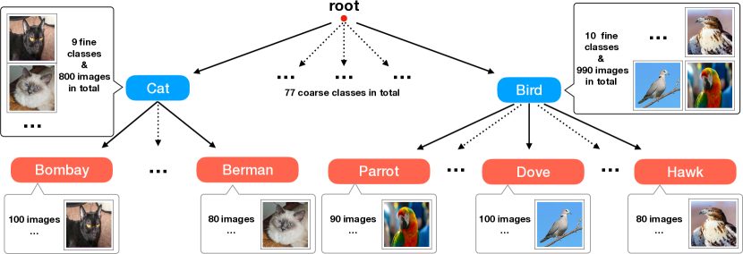
Figure 1: A many-class few-shot learning (MCFS) problem using multi-label class hierarchy information. There are a few coarse classes (blue) and each coarse class covers a large number of fine classes (red) so that the total number of fine classes is large. Only a few training samples are available for each fine class. The goal is to train a classifier to generate a prediction over all fine classes with the help of coarse prediction. We utilize meta-learning to solve the problem of many-class few-shot learning problem, where each task is an MCFS problem sampled from a certain distribution. The meta-learner’s goal is to help train a classifier for any sampled task with better adaptation to few-shot data within the sampled task.

Although previous works of fully supervised learning have shown the remarkable power of DNN when “many-class many-shot” training data is available, their performance degrades dramatically when each class only has a few samples available for training. In practical applications, acquiring samples of rare species or personal data from edge devices is usually difficult, expensive, and forbidden due to privacy protection. In many-class cases, annotating even one additional sample per class can be very expensive and requires a lot of human efforts. Moreover, the training set cannot be fully balanced over all the classes in practice. In these few-shot learning scenarios, the capacity of a deep model cannot be fully utilized, and it becomes much harder to generalize the model to unseen data. Recently, several approaches have been proposed to address the few-shot learning problem. Most of them are based on the idea of “meta-learning”, which trains a meta-learner over different few-shot tasks so it can generalize to new few-shot tasks with unseen classes. Thereby, the meta-learner aims to learn a stronger prior encoding the general knowledge achieved during learning various tasks, so it is capable to help a learner model quickly adapt to a new task with new classes of insufficient training samples. Meta-learning can be categorized into two types: methods based on “learning to optimize”, and methods based on metric learning. The former type adaptively modifies the optimizer (or some parts of it) used for training the task-specific model. It includes methods that incorporate an Recurrent Neural Networks (RNN) meta-learner [3, 4, 5], and model-agnostic meta-learning (MAML) methods aiming to learn a generally compelling initialization [6]. The second type learns a similarity/distance metric [7] or a model generating a support set of samples [8] that can be used to build K-Nearest Neighbors (KNN) classifiers from few-shot data in different tasks.

Instead of meta-learning methods, data augmentation based approaches, such as the hallucination method proposed in [9], address the few-shot learning problem by generating more artificial samples for each class. However, most existing few-shot learning approaches only focus on “few-class” cases (e.g., $5$ or $10$) per task, and their performance drastically collapses when the number of classes slightly grows to tens to hundreds. This is because the samples per class no longer provide enough information to distinguish them from other possible samples within a large number of other classes. And in real-world few-shot problems, a task is usually complicated involving many classes.

Fortunately, in practice, multi-outputs/labels information such as coarse-class labels in a class hierarchy is usually available or cheaper to obtain. In this case, the correlation between fine and coarse classes can be leveraged in solving the MCFS problem, e.g., by training a coarse-to-fine hierarchical prediction model. As shown in Fig. 1, coarse class labels might reveal the relationships among the targeted fine classes. Moreover, the samples per coarse class are sufficient to train a reliable coarse classifier, whose predictions are able to narrow down the candidates for the corresponding fine class. For example, a sheepdog with long hair could be easily mis-classified as a mop when training samples of sheepdog are insufficient. However, if we could train a reliable dog classifier, it would be much simpler to predict an image as a sheepdog than a mop given a correct prediction of the coarse class as “dog”. Training coarse-class prediction models is much easier and less suffered from the “many class few shot”problem (since the coarse classes are fewer than the fine classes and the samples per coarse class are much more than that for each fine class). It provides helpful information to fine-class prediction due to the relationship between coarse classes and fine classes. Hence, class hierarchy might provide weakly supervised information to help solve the “many-class few-shot (MCFS)” problem in a framework of multi-output learning, which aims to predict the class label on each level of the class hierarchy.

In this paper, we address the MCFS problem in both traditional supervised learning and in meta-learning settings by exploring the multi-output information on multiple class hierarchy levels. We develop a neural network architecture “memory-augmented hierarchical-classification networks (MahiNet)” that can be applied to both learning settings. MahiNet uses a Convolutional Neural Network (CNN), i.e., ResNet [1], as a backbone network to firstly extract features from raw images. It then trains coarse-class and fine-class classifiers based on the features, and combines their outputs to produce the final probability prediction over the fine classes. In this way, both the coarse-class and the fine-class classifiers mutually help each other within MahiNet: the coarse classifier helps to narrow down the candidates for the fine classifier, while the fine classifier provides multiple attributes describing every coarse class and can regularize the coarse classifier. This design leverages the relationship between the fine classes as well as the relationship between the fine classes and the coarse classes, which mitigates the difficulty caused by the “many class” challenge. To the best of our knowledge, we are the first to successfully train a multi-output model to employ existing class hierarchy prior for improving both few-shot learning and supervised learning. It is different from those methods discussed in related works that use a latent clustering hierarchy instead of the explicit class hierarchy we use. In Table I, we provide a brief comparison of MahiNet with other popular models on the learning scenarios they excel.

To address the “few-shot” problem, we apply two types of classifiers in MahiNet, i.e., MLP classifier and KNN classifier, which respectively have advantages in many-shot and few-shot situations. In principle, we always use MLP for coarse classification, and KNN for fine classification. Specially, with a sufficient amount of data in supervised learning, MLP is combined with KNN for fine classification; and in meta-learning when less data is available, we also use KNN for coarse classification to assist MLP.

To make the KNN learnable and adaptive to new classes with few-shot data, we train an attention module to provide the similarity/distance metric used in KNN, and a re-writable memory of limited size to store and update the KNN support set during training. In supervised learning, it is necessary to maintain and update a relatively small memory (e.g., 7.2% of the dataset in our experiment) by selecting a few representative samples, because conducting a KNN search over all available training samples is too expensive in computation. In meta-learning, the attention module can be treated as a meta-learner that learns a universal similarity metric across different tasks.

Since the commonly used datasets in meta-learning do not have hierarchical multi-label annotations, we randomly extract a large subset of ImageNet [10] “mcfsImageNet” as a benchmark dataset specifically designed for MCFS problem. Each sample in mcfsImageNet has two labels: a coarse class label and a fine class label. It contains 139,346 images from $77$ non-overlapping coarse classes composed of $754$ randomly sampled fine classes, each has only $\approx 180$ images, which might be further splitted for training, validation and test. The imbalance between different classes in the original ImageNet are preserved to reflect the imbalance in practical problems. Similarly, we further extract “mcfsOmniglot” from Omniglot [11] for the same purpose. We will make them publicly available later. In fully supervised learning experiments on these two datasets, MahiNet outperforms the widely used ResNet [1] (for fairness, MahiNet uses the same network (i.e., ResNet) as its backbone network). In meta-learning scenario where each test task covers many classes, it shows more promising performance than popular few-shot methods including prototypical networks [8] and relation networks [12], which are specifically designed for few-shot learning.

Our contributions can be concluded as: In the new version, we conclude our contributions at the end of introduction as follows: Our contributions can be concluded as: 1) We address a new problem setting called “many-class few-shot learning (MCFS)” that has been widely encountered in practice. Compared to the conventional “few-class few-shot (as in most few-shot learning methods)” or “many-class many-shot (as in most supervised learning methods)” settings, MCFS is more practical and challenging but has been rarely studied in the ML community. 2) To alleviate the challenge of “many-class few-shot”, we propose to utilize the knowledge of a predefined class hierarchy to train a model that takes the relationship between classes into account when generating a classifier over a relatively large number of classes. 3) To empirically justify whether our model can improve the MCFS problem by using class hierarchy information, we extract two new datasets from existing benchmarks, each coupled with a class hierarchy on reasonably specified classes. In experiments, we show that our method outperforms the other baselines in MCFS setting.

2 Related Works

2.1 Few-shot Learning

Generative models [13] were trained to provide a global prior knowledge for solving the one-shot learning problem. With the advent of deep learning techniques, some recent approaches [14, 15] use generative models to encode specific prior knowledge, such as strokes and patches. More recently, works in [9] and [16] have applied hallucinations to training images and to generate more training samples, which converts a few-shot problem to a many-shot problem.

Meta-learning has been widely studied to address the few-shot learning problems for fast adaptation to new tasks with only few-shot data. Meta-learning was first proposed in the last century [17, 18], and has recently brought significant improvements to few-shot learning, continual learning and online learning [19]. For example, the authors of [20] proposed a dataset of characters “Omniglot” for meta-learning while the work in [21] apply a Siamese network to this dataset. A more challenging dataset “miniImageNet” [5, 7] was introduced later. miniImageNet is a subset of ImageNet [10] and has more variety and higher recognition difficulty compared to Omniglot. Researchers have also studied a combination of RNN and attention based method to overcome the few-shot problem [5]. More recently, the method in [8] was proposed based on metric learning to learn a shared KNN [22] classifier for different tasks. In contrast, the authors of [6] developed their approach based on the second order optimization where the model can adapt quickly to new tasks or classes from an initialization shared by all tasks. The work in [23] addresses the few-shot image recognition problem by temporal convolution, which sequentially encodes the samples in a task. More recently, meta-learning strategy has been studied to solve other problems and tasks, such as using meta-learning training strategy to help design a more efficient unsupervised learning rule [24]; mitigating the low-resource problems in neural machine translation task [25]; alleviating the few annotations problem in object detection problem [26].

Our model is closely related to prototypical networks, in which every class is represented by a prototype that averages the embedding of all samples from that class, and the embedding is achieved by applying a shared encoder, i.e., the meta-learner. It can be modified to generate an adaptive number of prototypes [27] and to handle extra weakly-supervised labels [28, 29] on a category graph. Unlike these few-shot learning methods that produces a KNN classifier defined by the prototypes, our model produces multi-labels or multi-output predictions by combining the outputs of an MLP classifier and a KNN classifier, which are trained in either supervised learning or few-shot learning settings.

2.2 Multi-Label Classification

Multi-label classification aims to assign multiple class labels to every sample [30]. One solution is to use a chain of classifiers to turn multi-label problem into several binary classification problems [31, 32, 33]. Another solution treats multi-label classification as multi-class classification over all possible subsets of labels [34]. Other works learn an embedding or encoding space using metric learning approaches [35], feature-aware label space encoding, label propagation, etc. The work in [36] proposes a decision trees method for multi-label annotation problems. The efficiency can be improved by using an ensemble of a pruned set of labels [37]. The applications include multi-label classification for textual data [38], multi-label learning from crowds [39] and disease resistance prediction [40]. Our approach differs from these works in that the multi-output labels and predictions serve as auxiliary information to improve the many-class few-shot classification over fine classes.

2.3 Hierarchical Classification

Hierarchical classification is a special case of multi-label or multi-output problems [41, 42]. It has been applied to traditional supervised learning tasks [43], such as text classification [44, 45], community data [46], case-based reasoning [47], popularity prediction [48], supergraph search in graph databases [49], road networks [50], image annotation and robot navigation. However, to the best of our knowledge, our paper is the first work successfully leveraging class hierarchy information in few-shot learning and meta-learning tasks. Previous methods such as [51], have considered the class hierarchy information but failed to achieve improvement and thus did not integrate it in their method, whereas our method successfully leverage the hierarchical relationship between classes to improve the classification performance by using a memory-augmented model.

Similar idea of using hierarchy for few-shot learning has been studied in [52, 53], which learns to cluster semantic information and task representation, respectively. [28] utilizes coarsely labeled data in the hierarchy as weakly supervised data rather than multi-label annotations for few-shot learning. In computational biology, hierarchy information has also been found helpful in gene function prediction, where two main taxonomies are Gene Ontology and Functional Catalogue. [54] proposed a truth path rule as an ensemble method to govern both taxonomies. [55] shows that the key factors for the success of hierarchical ensemble methods are: (1)the integration and synergy among multi-label hierarchy, (2) data fusion, (3) cost-sensitive approaches, and (4) the strategy of selecting negative examples. [56] and [57] address the incomplete annotations of proteins using label hierarchy (as studied in this paper) by following the idea of few-shot learning. Specifically, they learn to predict the new gene ontology annotations by Bi-random walks on a hybrid graph [56] and downward random walks on a gene ontology [57], respectively.

3 Targeted Problem and Proposed Model

In this section, we first introduce the formulation of many-class few-shot problem in Sec. 3.1. Then we generally elaborate our network architecture in Sec. 3.2. Details for how to learn a similarity metric for a KNN classifier with attention module and how to update the memory (as a support set of the KNN classifier) are given in Sec. 3.3 and Sec. 3.4 respectively.

3.1 Problem Formulation

We study supervised learning and meta-learning. Given a training set of $n$ samples ${\mathbb{D}}=\{({\bm{x}}_{i},y_{i},z_{i})\}_{i=1}^{n}$, where each sample ${\bm{x}}_{i}\in{\mathbb{X}}$ is associated with multiple labels. For simplicity, we assume that each training sample is associated with two labels: a fine-class label $y_{i}\in\mathbb{Y}$ and a coarse-class label $z_{i}\in{\mathbb{Z}}$. The training data is sampled from a data set ${\mathbb{D}}$, i.e., $({\bm{x}}_{i},y_{i},z_{i})\sim{\mathbb{D}}$. Here, ${\mathbb{X}}$ denotes the set of samples; ${\mathbb{Y}}$ denotes the set of all the fine classes, and ${\mathbb{Z}}$ denotes the set of all the coarse classes. To define a class hierarchy for ${\mathbb{Y}}$ and ${\mathbb{Z}}$, we further assume that each coarse class $z\in{\mathbb{Z}}$ covers a subset of fine classes ${\mathbb{Y}}_{z}$, and that distinct coarse classes are associated with disjoint subsets of fine classes, i.e., for any $z_{1},~{}z_{2}\in{\mathbb{Z}}$, we have ${\mathbb{Y}}_{z_{1}}\cap{\mathbb{Y}}_{z_{2}}=\emptyset$. Our goal is fine-class classification by using the class hierarchy information and the coarse labels of the training data. In particular, the supervised learning setting in this case can be formulated as:

$$\min_{\Theta}\mathbb{E}_{({\bm{x}},y,z)\sim\mathcal{D}}-\log\Pr(y|{\bm{x}};\Theta),$$ (1)

where $\Theta$ is the model parameters and $\mathbb{E}$ refers to the expectation w.r.t. the data distribution. In practice, we solve the corresponding empirical risk minimization (ERM) during training, i.e.,

$$\min_{\Theta}\sum_{i=1}^{n}-\log\Pr(y_{i}|{\bm{x}}_{i};\Theta).$$ (2)

In contrast, meta-learning aims to learn a meta-learner model that can be applied to different tasks. Its objective is to maximize the expectation of the prediction likelihood of a task drawn from a distribution of tasks. Specifically, we assume that each task is the classification over a subset of fine classes $T$ sampled from a distribution $\mathcal{T}$ over all classes, and the problem is formulated as

$$\min_{\Theta}\mathbb{E}_{T\sim\mathcal{T}}\left[\mathbb{E}_{({\bm{x}},y,z)\sim{\mathbb{D}}_{T}}-\log\Pr(y|{\bm{x}};\Theta)\right],$$ (3)

where ${\mathbb{D}}_{T}$ refers to the set of samples with label $y_{i}\in T$. The corresponding ERM is

$$\min_{\Theta}\sum_{T}\left[\sum_{i\in\mathbb{D}_{T}}-\log\Pr(y_{i}|{\bm{x}}_{i};\Theta)\right],$$ (4)

where $T$ represents a task (defined by a subset of fine classes) sampled from distribution $\mathcal{T}$, and $\mathbb{D}_{T}$ is a training set for task $T$ sampled from ${\mathbb{D}}_{T}$.

To leverage the coarse class information of $z$, we write $\Pr(y|{\bm{x}};\Theta)$ in Eq. (1) and Eq. (3) as

$$\Pr(y|{\bm{x}};\Theta)=\sum_{z\in\mathcal{Z}}\Pr(y|z,{\bm{x}};\Theta_{f})\Pr(z|{\bm{x}};\Theta_{c}),$$ (5)

where $\Theta_{f}$ and $\Theta_{c}$ are the model parameters for fine classifier and coarse classifier, respectively. Accordingly, given a specific sample $({\bm{x}}_{i},y_{i},z_{i})$ with its ground truth labels for coarse and fine classes, we can write $\Pr(y_{i}|{\bm{x}}_{i};\Theta)$ in Eq. (2) and Eq. (4) as follows.

$$\Pr(y_{i}|{\bm{x}}_{i};\Theta)=\Pr(y_{i}|z_{i},{\bm{x}}_{i};\Theta_{f})\Pr(z_{i}|{\bm{x}}_{i};\Theta_{c}).$$ (6)

Suppose that a DNN model already produces a logit $a_{y}$ for each fine class $y$, and a logit $b_{z}$ for each coarse class $z$, the two probabilities in the right hand side of Eq. (6) are computed by applying softmax function to the logit values in the following way.

$$\Pr(y_{i}|z_{i},{\bm{x}}_{i};\Theta_{f})=\frac{\exp(a_{y_{i}})}{\sum_{y\in\mathcal{Y}_{z_{i}}}\exp(a_{y})},$$

$$\Pr(z_{i}|{\bm{x}}_{i};\Theta_{c})=\frac{\exp(b_{z_{i}})}{\sum_{z\in\mathcal{Z}}\exp(a_{z})}.$$ (7)

Therefore, we integrate multiple labels (both the fine-class label and coarse-class label) in an ERM, whose goal is to maximize the likelihood of the ground truth fine-class label. Given a DNN that produces two vectors of logits $a$ and $b$ for fine class and coarse class respectively, we can train the DNN for supervised learning or meta-learning by solving the ERM problems in Eq. (2) or Eq. (4) (with Eq. (6) and Eq. (3.1) plugged in).

3.2 Network Architecture

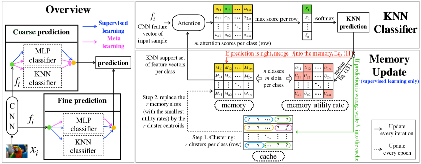
Figure 2: Left: MahiNet. The final fine-class prediction combines predictions based on multiple classes (both fine classes and coarse classes), each of which is produced by an MLP classifier or/and an attention-based KNN classifier. Top right: KNN classifier with learnable similarity metric and updatable support set. Attention provides a similarity metric $a_{j,k}$ between each input sample ${\bm{f}}_{i}$ and a small support set per class stored in memory ${\bm{M}}_{j,k}$. The learning of KNN classifier aims to optimize 1) the similarity metric parameterized by the attention, detailed in Sec. 3.3; and 2) a small support set of feature vectors per class stored in memory, detailed in Sec. 3.4. Bottom right: The memory update mechanism. In meta-learning, the memory stores the features of all training samples of a task. In supervised learning, the memory is updated during training as follows: for each sample ${\bm{x}}_{i}$ within an epoch, if the KNN classifier produces correct prediction, ${\bm{f}}_{i}$ will be merged into the memory; otherwise, ${\bm{f}}_{i}$ will be written into a “cache”. At the end of each epoch, we apply clustering to the samples per class stored in the cache, and use the resultant centroids to replace $r$ slots of the memory with the smallest utility rate [58].

To address MCFS problem in both supervised learning and meta-learning scenarios, we developed a universal model, MahiNet, as in Figure 2. MahiNet uses a CNN to extract features from raw inputs, and then applies two modules to produce coarse-class prediction and fine-class prediction, respectively. Each module includes one or two classifiers: either an MLP or an attention-based KNN classifier or both. Intuitively, MLP performs better when data is sufficient, while the KNN classifier is more stable in few-shot scenario. Hence, we always apply MLP to coarse prediction and always apply KNN to fine prediction. In addition, we use KNN to assist MLP for the coarse module in meta-learning, and use MLP to assist KNN for the fine module in supervised learning. We develop two mechanisms to make the KNN classifier learnable and be able to quickly adapt to new tasks in the meta-learning scenario. In the attention-based KNN classifier, an attention module is trained to compute the similarity between two samples, and a re-writable memory is maintained with a highly representative support set for KNN prediction. The memory is updated during training.

Our method for learning a KNN classifier combines the ideas from two popular meta-learning methods, i.e., matching networks [7] that aim to learn a similarity metric, and prototypical networks [8] that aim to find a representative center per class for NN search. However, our method relies on an augmented memory rather than a bidirectional RNN for retrieving of NN in matching networks. In contrast to prototypical networks, which only has one prototype per class, we allow multiple prototypes as long as they can fit in the memory budget. Together these two mechanisms prevent the confusion caused by subtle differences between classes in “many-class” scenario. Notably, MahiNet can also be extended to “life-long learning” given this memory updating mechanism. We do not adopt the architecture used in [23] since it requires the representations of all historical data to be stored.

3.3 Learn a KNN Similarity Metric with an Attention

In MahiNet, we train an attention module to compute the similarity used in the KNN classifier. The attention module learns a distance metric between the feature vector $f_{i}$ of a given sample ${\bm{x}}_{i}$ and any feature vector from the support set stored in the memory. Specifically, we use the dot product attention similar to the one adopted in [59] for supervised learning, and use an Euclidean distance based attention for meta-learning, following the instruction from [8]. Given a sample ${\bm{x}}_{i}$, we compute a feature vector ${\bm{f}}_{i}\in\mathbb{R}^{d}$ by applying a backbone CNN to ${\bm{x}}_{i}$. In the memory, we maintain a support set of $m$ feature vectors for each class, i.e., ${\bm{M}}\in\mathbb{R}^{C\times m\times d}$, where $C$ is the number of classes. The KNN classifier produces the class probabilities of ${\bm{x}}_{i}$ by first calculating the attention scores between ${\bm{f}}_{i}$ and each feature vector in the memory, as follows.

$$a({\bm{f}}_{i},{\bm{M}}_{j,k})=\frac{g({\bm{f}}_{i}){\cdot}h({\bm{M}}_{j,k})}{\|g({\bm{f}}_{i})\|\|h({\bm{M}}_{j,k})\|}$$

$$~{}~{}{\rm or}~{}~{}-\|g({\bm{f}}_{i})-h({\bm{M}}_{j,k})\|_{2},~{}~{}\forall j\in[C],~{}k\in[m],$$ (8)

where $g$ and $h$ are learnable transformations for ${\bm{f}}_{i}$ and the feature vectors in the memory.

We select the top $K$ nearest neighbors, denoted by $top_{k}$, of ${\bm{f}}_{i}$ among the $m$ feature vectors for each class $j$, and compute the sum of their similarity scores as the attention score of ${\bm{f}}_{i}$ to class $j$, i.e.,

$$s({\bm{f}}_{i},{\bm{M}}_{j})=\sum_{k\in[m]}top_{k}(a({\bm{f}}_{i},{\bm{M}}_{j,k})),~{}~{}\forall j\in[C].$$ (9)

We usually find $K=1$ is sufficient in practice. The predicted class probability is derived by applying a softmax function to the attention scores of ${\bm{f}}_{i}$ over all $C$ classes, i.e.,

$$\Pr(y_{i}=j)\triangleq\frac{\exp{(s({\bm{f}}_{i},{\bm{M}}_{j}))}}{\sum_{j^{\prime}=1}^{C}\exp{(s({\bm{f}}_{i},{\bm{M}}_{j^{\prime}}))}},~{}~{}\forall j\in[C].$$ (10)

3.4 Memory Mechanism for the Support Set of KNN

Ideally, the memory ${\bm{M}}\in\mathbb{R}^{C\times m\times d}$ can store all available training samples as the support set of the KNN classifier. In meta-learning, in each episode, we sample a task with $C$ classes and $m$ training samples per class, and store them in the memory. Due to the small amount of training data for each task, we can store all of them and thus do not need to update the memory. In supervised learning, we only focus on one task. This task usually has a large training set and it is inefficient, unnecessary and too computationally expensive to store all the training set in the memory. Hence, we set up a budget hyper-parameter $m$ for each class. $m$ is the maximal number of feature vectors to be stored in the memory for one class. Moreover, we develop a memory update mechanism to maintain a small memory with diverse and representative feature vectors per class (t-SNE visualization of the diversity and representability of the memory can be found in the experiment section.). Intuitively, it can choose to forget or merge feature vectors that are no longer representative, and select new important feature vectors into memory.

We will show later in experiments that a small memory can result in sufficient improvement, while the time cost of memory updating is negligible. Accordingly, the memory in meta-learning does not need to be updated according to a rule, while in supervised learning, we design the writing rule as follows. During training, for the data that can be correctly predicted by the KNN classifier, we merge its feature with corresponding slots in the memory by computing their convex combination, i.e.,

$${\bm{M}}_{j,k}=\{\begin{array}[]{ll}\gamma\times{\bm{M}}_{j,k}+(1-\gamma)\times{\bm{f}}_{i},&\text{if }\hat{y}_{i}=y_{i}\\ {\bm{M}}_{j,k},&\text{otherwise}\\ \end{array},$$ (11)

where $y_{i}$ is the ground truth label, and $\gamma=0.95$ is a combination weight that works well in most of our empirical studies; for input feature vector that cannot be correctly predicted, we write it to a cache ${\mathbb{C}}=\{{\mathbb{C}}_{1},...,{\mathbb{C}}_{C}\}$ that stores the candidates written into the memory for the next epoch, i.e.,

$${\mathbb{C}}_{j}=\{\begin{array}[]{ll}{\mathbb{C}}_{j},&\text{if }\hat{y}_{i}=y_{i}\\ {\mathbb{C}}_{j}\cup\{{\bm{f}}_{i}\},&\text{otherwise}\\ \end{array},$$ (12)

Concurrently, we record the utility rate of the feature vectors in the memory, i.e., how many times each feature vector being selected into the $K$ nearest neighbor during the epoch. The rates are stored in a matrix ${\bm{U}}\in\mathbb{R}^{C\times m}$, and we update it as follows.

$${\bm{U}}_{j,k}=\{\begin{array}[]{ll}{\bm{U}}_{j,k}\times\mu,&\text{if }\hat{y}_{i}=y_{i}\\ {\bm{U}}_{j,k}\times\eta,&\text{otherwise}\\ \end{array},$$ (13)

where $\mu\in(1,2)$ and $\eta\in(0,1)$ are hyper-parameters.

At the end of each epoch, we apply clustering to the feature vectors per class in the cache, and obtain $r$ cluster centroids as the candidates for memory update in the next epoch. Then, for each class, we replace $r$ feature vectors in the memory that have the smallest utility rate with the $r$ cluster centroids.

Algorithm 1 Training MahiNet for Supervised Learning

0:  Training set ${\mathbb{D}}=\{({\bm{x}}_{i},y_{i},z_{i})\}_{i=1}^{n}$;     Randomly initialized $\theta_{f}^{KNN}$, pre-trained $\theta^{CNN}$, $\theta_{c}^{MLP}$ and $\theta_{f}^{MLP}$;      Hyper-parameters: memory update parameters $r$, $\gamma$, $\mu$ and $\eta$; learning rate and its scheduler;

1:  while no converge do

2:     for mini-batch $\{({\bm{x}}_{i},y_{i},z_{i})\}_{i\in B}$ in ${\mathbb{D}}$ do

3:        Compute fine-class logits $a$ and coarse-class logits $b$ from the outputs of MLP/KNN classifiers;

4:        Apply one step of mini-batch SGD for ERM in Eq. (2) (with Eq. (6) and Eq. (3.1) plugged in);

5:        for sample in the mini-batch do

6:           Update the memory ${\bm{M}}$ according to Eq. (11);

7:           Update the utility rate ${\bm{U}}$ according to Eq. (13);

8:           Expand the feature cache ${\mathbb{C}}$ according to Eq. (12);

9:        end for

10:     end for

11:     for each fine class $j$ in $\mathcal{Y}$ do

12:        Find the indexes of the $r$ smallest values in ${\bm{U}}_{j}$, denoted as $\{k_{1},k_{2},...,k_{r}\}$;

13:        Clustering of the feature vectors within cache ${\mathbb{C}}_{j}$ to $r$ clusters with centroids $\{c_{1},c_{2},...,c_{r}\}$;

14:        Replace the $r$ memory slots by centroids: ${\bm{M}}_{j,k_{i}}=c_{i}$ for $i\in[r]$;

15:     end for

16:  end while

4 Training Strategies

As shown in the network structure in Fig. 2, in supervised learning and meta-learning, we use different combinations of MLP and KNN to produce the multi-output predictions of fine-class and coarse-class. The classifiers are combined by summing up their output logits for each class, and a softmax function is applied to the combined logits to generate the class probabilities. Assume the MLP classifiers for the coarse classes and the fine classes are $\phi(\cdot;\theta_{c}^{MLP})$ and $\phi(\cdot;\theta_{f}^{MLP})$, the KNN classifiers for the coarse classes and the fine classes are $\phi(\cdot;\theta_{c}^{KNN})$ and $\phi(\cdot;\theta_{f}^{KNN})$. In supervised learning, the model parameters are $\theta^{CNN}$, $\Theta_{c}=\theta_{c}^{MLP}$ and $\Theta_{f}=\{\theta_{f}^{MLP},\theta_{f}^{KNN}\}$; in meta-learning setting, the model parameters are $\theta^{CNN}$, $\Theta_{c}=\{\theta_{c}^{MLP},\theta_{c}^{KNN}\}$ and $\Theta_{f}=\theta_{f}^{KNN}$.

According to Sec. 3.1, we train MahiNet for supervised learning by solving the ERM problem in Eq. (2). For meta-learning, we instead train MahiNet by solving Eq. (4). As previously mentioned, the multi-output logits (for either fine classes or coarse classes) used in those ERM problems are obtained by summing up the logits produced by the corresponding combination of the classifiers.

4.1 Training MahiNet for Supervised learning

In supervised learning, the memory update relies heavily on the clustering of the merged feature vectors in the cache. To achieve relatively high-quality feature vectors, we first pre-train the CNN+MLP model by using standard backpropagation, which minimizes the sum of cross entropy loss on both the coarse-classes and fine-classes. The loss is computed based on the logits of fine-classes and the logits of coarse-classes, which are the outputs of the corresponding MLP classifiers. Then, we fint-tune the whole model, which includes the fine-class KNN classifier, with memory update applied. Specifically, in every iteration, we firstly update the parameters of the model with mini-batch SGD based on the coarse-level and fine-level logits produced by the MLP and KNN classifiers. Then, the memory that stores a limited number of representative feature maps for every class is updated by the rules explained in Sec. 3.4, as well as the associated utility rates and feature cache. The details of the training procedure during the fine-tune stage is explained in Alg. 1.

Algorithm 2 Training MahiNet for Meta-Learning

0:  Training set ${\mathbb{D}}=\{({\bm{x}}_{i},y_{i},z_{i})\}_{i=1}^{n}$ and fine class set ${\mathbb{Y}}$;     Parameters: randomly initialized $\theta^{CNN}$, $\theta_{c}^{MLP}$, $\theta_{f}^{MLP}$, and $\theta_{f}^{KNN}$;      Hyper-parameters: learning rate, scheduler; for each class, number of queries $n_{s}$, support set size $n_{S}$;

1:  while not converge do

2:     Sample a task $T\sim\mathcal{T}$ as a subset of fine classes $T\subseteq{\mathbb{Y}}$.

3:     for class $j$ in $T$ do

4:        Randomly sample $n_{s}$ data points of class $j$ from ${\mathbb{D}}$ to be the support set ${\mathbb{S}}_{j}$ of class $j$.

5:        Randomly sample $n_{q}$ data points of class $j$ from ${\mathbb{D}}\backslash{\mathbb{S}}_{j}$ to be the query set ${\mathbb{Q}}_{j}$ of class $j$.

6:     end for

7:     for mini-batch from ${\mathbb{Q}}$ do

8:        Compute fine-class logits $a$ and coarse-class logits $b$ from the outputs of MLP/KNN classifiers;

9:        Apply one step of mini-batch SGD for ERM in Eq. (4) (with Eq. (6) and Eq. (3.1) plugged in);

10:     end for

11:  end while

TABLE II: Comparison of the statistics for mcfsImageNet, mcfsOmniglot and previously popular datasets for supervised learning and few-shot learning. We propose datasets mcfsImageNet, mcfsOmniglot, in which every image is annotated by multiple labels: a coarse label and a fine label. “#c” and “#f” denote the number of coarse classes and fine classes, respectively. “-” means “not applicable”.

	Meta-Learning						Supervised Learning				#image	image size
	Train		Val		Test		Train		Test
	#c	#f	#c	#f	#c	#f	#c	#f	#c	#f
ImageNet-1k	-	-	-	-	-	-	1	1000	1	1000	1.43M	224
miniImageNet	1	64	1	16	1	20	-	-	-	-	0.06M	84
Omniglot	33	1028	5	172	13	423	-	-	-	-	0.03M	28
mcfsOmniglot	50	973	50	244	50	1624	-	-	-	-	0.03M	28
mcfsImageNet	77	482	61	120	68	152	77	754	77	754	0.14M	112

4.2 Training MahiNet for Meta-learning

When sampling the training/test tasks, we allow unseen fine classes that were not covered in any training task to appear in test tasks, but we fix the ground set of the coarse classes for both training and test tasks. Hence, every coarse class appearing in any test task has been seen during training, but the corresponding fine classes belonging to this coarse class in training and test tasks can be vary.

In the meta-learning setting, since the tasks in different iterations targets samples from different subsets of classes and thus ideally need different feature map representations [60], we do not maintain the memory during training so every class can have a fixed representation. Instead, the memory is only maintained within each iteration for a specific task and it stores feature map representations extracted from the support set of the task. The detailed training procedure can be found in Alg. 2. In summary, we generate a training task by randomly sampling a subset of fine classes, and then we randomly sample a support set ${\mathbb{S}}$ and a query set ${\mathbb{Q}}$ from the associated samples belonging to these classes. We store the CNN feature vectors of ${\mathbb{S}}$ in the memory, and train MahiNet to produce correct predictions for the samples in ${\mathbb{Q}}$ with the help of coarse label predictions.

5 Experiments

In this section, we first introduce two new benchmark datasets specifically designed for MCFS problem, and compare them with other popular datasets in Sec. 5.1. Then, we show that MahiNet has better generality and can outperform the specially designed models in both supervised learning (in Sec. 5.2) and meta-learning (in Sec. 5.3) scenarios. We also present an ablation study of MahiNet to show the improvements brought by different components and how they interact with each other. In Sec. 5.4, we report the comparison with the variants of baseline models in order to show the broad applicability of our strategy of leveraging the hierarchy structures. In Sec. 5.6, we present an analysis of the computational costs caused by the augmented memory in MahiNet.

5.1 Two New Benchmarks for MCFS Problem: mcfsImageNet & mcfsOmniglot

Since existing datasets for both supervised learning and meta-learning settings neither support multiple labels nor fulfill the requirement of “many-class few-shot” settings, we propose two novel benchmark datasets specifically for MCFS Problem, i.e., mcfsImageNet & mcfsOmniglot. The samples in them are annotated by multiple labels of different granularity. We compare them with several existing datasets in Table II. Our following experimental study focuses on these two datasets.

ImageNet [10] is one of the most widely used large-scale benchmark dataset for image classification. Although it provides hierarchical information about class labels, it cannot be directly used to test the performance of MCFS learning methods. One main reason is that a fine class in ImageNet may belong to multiple coarse classes, which introduces unnecessary noise in narrowing down the fine-class candidates and is outside the scope of MCFS problem, in which each sample has only one unique coarse-class label. In addition, ImageNet does not satisfy the criteria of “few-shot” per class: it has around 1,430 images per class on average. miniImageNet [7] is a widely used benchmark dataset in meta-learning community to test the performance on few-shot learning tasks. miniImageNet is a subset extracted from ImageNet; however, its data are collected from only $80$ fine classes, which is much less than “many-class” usually refers to in practice. In addition, it does not provide an associated class hierarchy.

Hence, to develop a benchmark dataset specifically for the purpose of testing the performance of MCFS learning, we extracted a subset of images from ImageNet and created a dataset called “mcfsImageNet”. Table II compares the statistics of mcfsImageNet with several benchmark datasets. Comparing to the original ImageNet, we avoided selecting the samples that belong to more than one coarse classes into mcfsImageNet in order to meet the class hierarchy requirements of MCFS problem, i.e., each fine class only belongs to one coarse class. Compared to miniImageNet, mcfsImageNet is about $5\times$ larger, and covers $754$ fine classes in total, which is much more than the $80$ fine classes in miniImageNet. Moreover, on average, each fine class only has $\sim 185$ images for training and test, which matches the typical MCFS scenarios in practice. Additionally, the number of coarse classes in mcfsImageNet is $77$, which is much less than $754$ of the fine classes. This is consistent with the data properties found in many practical applications, where the coarse-class labels can only provide weak supervision, but each coarse class has sufficient training samples. Further, we avoided selecting coarse classes which are too broad or contain too many different fine classes. For example, the “Misc” class in ImageNet has $20400$ sub-classes, and includes both animal ($3998$ sub-classes) and plant ($4486$ sub-classes). This kind of coarse label covers too many classes and cannot provide valuable information to distinguish different fine classes.

Omniglot [11] is a small hand-written character dataset with two-level class labels. However, in their original training/test splitting, the test set contains new coarse classes that are not covered by the training set, since this weakly labeled information is not supposed to be utilized during the training stage. This is inconsistent with the MCFS settings, in which all the coarse classes are exposed in training, but new fine classes can still emerge during test. Therefore, we re-split Omniglot to fulfill the MCFS problem requirement.

5.2 Supervised Learning Experiments

TABLE III: The performance (test accuracy) comparison of different models in the setting of supervised learning on mcfsImageNet.

Model	Hierarchy	#Params (MB)	Accuracy
Prototypical Net [8]	N	11	2.7%
ResNet18 [1]	N	11	48.6%
MahiNet w/o KNN	Y	11	49.1%
MahiNet (ours)	Y	12	49.9%

TABLE IV: Test accuracy (%) of different approaches in meta-learning scenario on mcfsImageNet. Both the average accuracy over 600 test episodes and the corresponding 95% confidence intervals are reported. In the first row, “n-k” represents $n$-way (class) $k$-shot classification task. e.g., “20-10” refers to “20-way 10-shot”. To make a fair comparison, all models use the same backbone: ResNet18. In 50-way experiments, Relation Net stops to improve after the first few iterations and fails to achieve comparable performance (more details in Sec. 5.4).

Model	Hierarchy	#params (MB)	5-10	20-5	20-10	50-5	50-10
ResNet18[1]	N	11	60.7	58.6	67.2	48.9	56.8
Prototypical Net[8]	N	11	78.48$\pm$0.66	67.78$\pm$0.37	70.11$\pm$0.38	57.74$\pm$0.24	62.12$\pm$0.24
Relation Net[12]	N	11	74.12$\pm$0.78	52.66$\pm$0.43	55.45$\pm$0.46	N/A	N/A
MAML[6]	N	11	61.67$\pm$0.01	47.24$\pm$0.01	48.10$\pm$0.00	11.43$\pm$0.00	11.88$\pm$0.00
Reptile[61]	N	11	36.21$\pm$0.01	29.13$\pm$0.01	15.23$\pm$0.01	18.03$\pm$0.00	9.16$\pm$0.00
MahiNet (Ours)	Y	12	80.74$\pm$0.66	70.11$\pm$0.41	73.50$\pm$0.36	58.80$\pm$0.24	62.80$\pm$0.24

TABLE V: Ablation studies of MahiNet in the meta-learning setting. Both the average accuracy over 600 test episodes and the corresponding 95% confidence intervals are reported. In the first row, “n-k” represents $n$-way (class) $k$-shot classification task. “Mem-1” stores the average feature of all training samples for each class in one task; “Mem-2” stores all features of the training samples in one task.

Memory		Attention	Hierarchy	MLP-classifier	KNN-classifier	5-10	20-5	20-10	50-5	50-10
Mem-1	Mem-2
$\checkmark$				$\checkmark$	$\checkmark$	79.04$\pm$0.67	68.46$\pm$0.38	71.13$\pm$0.38	58.09$\pm$0.24	62.18$\pm$0.22
	$\checkmark$			$\checkmark$	$\checkmark$	77.41$\pm$0.71	66.89$\pm$0.40	71.72$\pm$0.37	55.25$\pm$0.23	59.38$\pm$0.23
	$\checkmark$	$\checkmark$		$\checkmark$	$\checkmark$	76.85$\pm$0.67	66.43$\pm$0.41	70.01$\pm$0.38	55.13$\pm$0.23	59.22$\pm$0.23
$\checkmark$	$\checkmark$	$\checkmark$		$\checkmark$	$\checkmark$	78.27$\pm$0.68	67.03$\pm$0.41	71.20$\pm$0.37	57.98$\pm$0.24	62.40$\pm$0.23
$\checkmark$	$\checkmark$	$\checkmark$	$\checkmark$		$\checkmark$	79.61$\pm$0.67	69.49$\pm$0.40	72.52$\pm$0.37	58.48$\pm$0.24	62.62$\pm$0.24
$\checkmark$	$\checkmark$	$\checkmark$	$\checkmark$	$\checkmark$		79.06$\pm$0.66	69.10$\pm$0.41	72.15$\pm$0.36	58.30$\pm$0.23	62.51$\pm$0.24
$\checkmark$		$\checkmark$	$\checkmark$	$\checkmark$	$\checkmark$	80.64$\pm$0.64	68.99$\pm$0.40	72.78$\pm$0.37	58.56$\pm$0.25	62.70$\pm$0.24
$\checkmark$	$\checkmark$	$\checkmark$	$\checkmark$	$\checkmark$	$\checkmark$	80.74$\pm$0.66	70.11$\pm$0.41	73.50$\pm$0.36	58.80$\pm$0.24	62.80$\pm$0.24

5.2.1 Setup

We use ResNet18 [1] as the backbone CNN. The transformation functions $g$ and $h$ in the attention module are two fully connected layers followed by group normalization [62] with a residual connection. We set the memory size to $m=12$ and the number of clusters to $r=3$, which can achieve a better trade-off between the memory cost and performance. Batch normalization [63] is applied after each convolution and before activation. During pre-training, we apply the cross entropy loss on the probability predictions in Eq. (3.1). During fine-tuning, we fix the $\theta^{CNN}$, $\theta^{MLP}_{c}$, and $\theta_{f}^{MLP}$ to ensure the fine-tuning process is stable. We use SGD with a mini-batch size of $128$ and a cosine learning rate scheduler with an initial learning rate $0.1$. $\mu=1.05$, $\eta=0.95$, a weight decay of $0.0001$, and a momentum of $0.9$ are used. We train the model for $100$ epochs during pre-training and $90$ epochs for the fine-tuning. All hyperparameters are tuned on 20% samples randomly sampled from the training set. we use 20% data randomly sampled from the training set to serve as the validation set to tune all the hyperparameters.

5.2.2 Experiments on mcfsImageNet

Table III compares MahiNet with the supervised learning model (i.e., ResNet18) and meta-learning model (i.e., prototypical networks) in the setting of supervised learning. The results show that MahiNet outperforms the specialized models, such as ResNet18 in MCFS scenario.

We also show the number of parameters for every method, which indicates that our model only has 9% more parameters than the baselines. Even using the version without KNN (which has the same number of parameters as baselines) can still outperform them.

Prototypical networks have been specifically designed for few-shot learning. Although it can achieve promising performance on few-shot tasks each covering only a few classes and samples, it fails when directly used to classify many classes in the classical supervised learning setting, as shown in Table III. A primary reason, as we discussed in Section 1, is that the resulted prototype suffers from high variance (since it is simply the average over an extremely few amount of samples per class) and cannot distinguish each class from tens of thousands of other classes (few-shot learning task only needs to distinguish it from 5-10 classes). Hence, dedicated modifications is necessary to make prototypical networks also work in the supervised learning setting. One motivation of this paper is to develop a model that can be trained and directly used in both settings.

The failure of Prototypical networks in supervised learning setting is not too surprising since for prototypical network the training and test task in the supervised setting is significantly different. We keep its training stage the same (i.e., target a task of 5 classes in every episode). In the test stage, we use the prototypes as the per-class means of training samples in each class to perform classification over all available classes on the test set data. Note the number of classes in the training tasks and the test task are significantly different, which introduces a large gap between training and test that leads to the failure. This can also be validated by observing the change on performance when we intentionally reduce the gap: the accuracy improves as the number of classes in each training task increases.

Another potential method to reduce the training-test gap is to increase the number of classes/ways per task to the same number of classes in supervised learning. However, prototypical net requires an prohibitive memory cost in such many class setting, i.e, it needs to keep 754(number of classes)$\times$2(1 for support set, 1 for query set)=1512 samples in memory for 1 shot learning setting and 754$\times$6(5 for support set, 1 for query set) = 4536 samples for 5 shots setting. Unlike classical supervised learning models which only needs to keep the model parameters in memory, prototypical net needs to build prototypes on the fly from the few-shot samples in the current episode, so at least one sample should be available to build the prototypes and at least one sample for query.

To separately measure the contribution of the class hierarchy and the attention-based KNN classifier, we conduct an ablation study that removes the KNN classifier from MahiNet. The results show that MahiNet still outperforms ResNet18 even when only using the extra coarse-label information and an MLP classifier for fine classes during training. Using a KNN classifier further improves the performance since KNN is more robust in the few-shot fine-level classifications. In supervised learning scenario, memory update is applied in an efficient way. 1) For each epoch, the average clustering time is 30s and is only $7.6\%$ of the total epoch time (393s). 2) Within an epoch, the memory update time (0.02s) is only $9\%$ of the total iteration time (0.22s).

5.3 Meta-Learning Experiments

5.3.1 Setup

We use the same backbone CNN (i.e., ResNet18) and transformation functions (i.e., $g$, and $h$) for attention as in supervised learning. In each task, we sample the same number of classes for training and test, and follow the training procedure in [8]. For a fair comparison, all baselines and our model are trained on the same number of classes for all training tasks, since increasing the number of classes in training tasks improves the performance as indicated in [8]. We initialize the learning rate as $10^{-3}$ and halve it after every 10k iterations. Our model is trained by ADAM [64] using a mini-batch size of $128$ (only in the pre-training stage), a weight decay of $0.0001$, and a momentum of $0.9$. We train the model for 25k iterations in total. Given the class hierarchy, the training objective sums up the cross entropy losses computed over the coarse class and over the fine classes, respectively. All hyper-parameters are tuned based on the validation set introduced in Table II. Every baseline and our method use the same training set and test test, and the test set is inaccessible during training so any data leakage is prohibited. In every experimental setting, we make the comparison fair by applying the same backbone, same training and test data, the same task setting (we follow the most popular N way K shot problem setting) and the same training strategy (including how to sample tasks and the value of N and K for meta-learning, since higher N and K generally lead to better performance as indicated in [8]).

5.3.2 Experiments on mcfsImageNet

Table IV shows that MahiNet outperforms the supervised learning baseline (ResNet18) and the meta-learning baseline (Prototypical Net). For ResNet18, we use the fine-tuning introduced in [6], in which the trained network is first fine-tuned on the training set (i.e., the support set) provided in the new task in the test stage and then tested on the associated query set. To evaluate the contributions of each component in MahiNet, we show results of several variants in Table V. “Attention” refers to the parametric functions for $g$ and $h$, otherwise we use identity mapping. “Hierarchy” refers to the assist of class hierarchy. For a specific task, “Mem-1” stores the average embedding over all training samples for each class in one task; “Mem-2” stores all the embeddings of the training samples in one task; “Mem-3” is the union of “Mem-1” and “Mem-2”. Table V implies: (1) Class hierarchy information can incur steady performance across all tasks; (2) Combining “Mem-1” and “Mem-2” outperforms using either of them independently; (3) Attention brings significant improvement to MCFS problem only when being trained with class hierarchy. Because the data is usually insufficient to train a reliable similarity metric to distinguish all fine classes, but distinguishing a few fine classes in each coarse class is much easier. The attention module is merely parameterized by the two linear layers $g$ and $h$, which are usually not expressive enough to learn the complex metric without the side information of class hierarchy. With the class hierarchy as a prior knowledge, the attention module only needs to distinguish much fewer fine classes within each coarse class, and the learned attention can faithfully reflect the local similarity within each coarse class. We also show the number of parameters for every method in the table. Our method only has 9% more parameters compared to baselines.

5.3.3 Experiments on mcfsOmniglot

We conduct experiments on the secondary benchmark mcfsOmniglot. We use the same training setting as for mcfsImageNet. Following [65], mcfsOmniglot is augmented with rotations by multiples of 90 degrees. In order to make an apple-to-apple comparison to other baselines, we follow the same backbone used in their experiments. Therefore, we use four consecutive convolutional layers, each followed by a batch normalization layer, as the backbone CNN and compare MahiNet with prototypical networks as in Table VI. We do ablation study on MahiNet with/without hierarchy and MahiNet with different kinds of memory. “Mem-3”, i.e., the union of “Mem-1” and “Mem-2”, outperforms “Mem-1”, and “Attention” mechanism can improve the performance. Additionally, MahiNet outperforms other compared methods, which indicates the class hierarchy assists to make more accurate predictions. In summary, experiments on the small-scale and large-scale datasets show that class hierarchy brings a stable improvement.

TABLE VI: Test accuracy (%) of basedline, our method and its variants in the meta-learning scenario on mcfsOmniglot. Both the average accuracy over 600 test episodes and the corresponding 95% confidence intervals are reported. In the first row, “n-k” represents $n$-way (class) $k$-shot classification task. e.g., “20-10” refers to “20-way 10-shot”.

Model	Hierarchy	5-5	20-5	50-5
Reptile [61]	N	54.70$\pm$0.02	17.10$\pm$0.01	8.34$\pm$0.02
MAML [6]	N	74.60$\pm$0.01	21.61$\pm$0.00	9.27$\pm$0.20
Prototypical Net [8]	N	99.10$\pm$0.15	98.84$\pm$0.11	97.94$\pm$0.08
MahiNet (Mem-1)	N	99.17$\pm$0.16	98.82$\pm$0.11	97.96$\pm$0.09
MahiNet (Mem-3)	N	99.31$\pm$0.18	98.89$\pm$0.11	97.93$\pm$0.09
MahiNet (Mem-3)	Y	99.40$\pm$0.15	99.00$\pm$0.16	98.10$\pm$0.17

5.4 Comparison to Variants of Relation Net

5.4.1 Relation network with class hierarchy

In order to demonstrate that the class hierarchy information and the multi-output model not only improves MahiNet but also other existing models, we train relation network with class hierarchy in the similar manner as we train MahiNet. The results are shown in Table  VII. It indicates that the class hierarchy also improves the accuracy of relation network by more than $1\%$, which verifies the advantage and generality of using class hierarchy in other models. Although the relation net with class hierarchy achieves a better performance, MahiNet still outperforms this improved variant due to its advantage in its model architecture, which are specially designed for utilizing the class hierarchy in the many-class few-shot scenario.

TABLE VII: The improvement of class hierarchy on relation network on mcfsImageNet. The average test accuracy over 600 test episodes and the corresponding 95% confidence intervals are reported.

Model	Hierarchy	5 way 5 shot	5 way 10 shot
Relation Net[12]	N	63.02$\pm$0.87	74.12$\pm$0.78
Relation Net	Y	66.82$\pm$0.86	75.31$\pm$0.90
MahiNet (Mem-3)	Y	74.98$\pm$0.75	80.74$\pm$0.66

5.4.2 Relation Network in many-class setting

When relation network is trained in many-class settings using the same training strategy from [12], we found that the network usually stops to improve and stays near a sub-optimal solution. Specifically, after the first few iterations, the training loss still stays at a high level and the training accuracy still stays low. They do not change too much even after hundreds of iterations, and this problem cannot be solved after trying different initial learning rates. The training loss quickly converges to around 0.02 and the training accuracy stays at $\sim 2\%$ no matter what learning rate is applied to the training procedure. Relation net on other low way settings have a competitive performance as shown in Table VII, which is also the settings reported in their papers. We use the same hyper-parameters as their paper for both few-class and many-class settings and the difference is only the parameter of the number of way. Even if relation network performs well in the few-class settings, its performance dramatically degrade when given the challenging high-way settings. One potential reason for this is that relation net uses MSE loss to regress the relation score to the ground truth: matched pairs have similarity 1 and mismatched pair have similarity 0. When the number of ways increases, the imbalance between the number of matched pairs and unmatched pairs grows and training is mainly to optimize the loss generated by the mismatched pairs instead of the matched ones, so that the objective focuses more on how to avoid mismatching instead of matching, i.e., predicting correctly, and makes the accuracy more difficult to get improvement. This suggests that relation networks may need more tricky way to train it successfully in a many-class setting compared to the few-class settings and traditional few-class few-shot learning approaches may not be directly applied in many-class few-shot problems. This is also one of the drawbacks for relation net and how to make the model more robust to hyper-parameter tuning is beyond the scope of our paper.

5.5 Analysis of Hierarchy

The main reasons of the improvement in our paper are: (1) our model can utilize prior knowledge from the class hierarchy; (2) we use an effective memory update scheme to iteratively and adaptively refine the support set. We show how much improvement the class hierarchy can bring to our model in Table V and to other baselines in Table～VII. The upper half of Table V are variants of our model without using hierarchy while the lower half are variants with hierarchy. It shows that the variants with hierarchy consistently outperform the ones without using hierarchy. To see whether hierarchy can help to improve other baselines, in Table～VII, we add hierarchy information to relation net (while keeping the other components the same) and it achieves 1-4% improvement on accuracy.

5.6 Analysis of Augmented Memory

5.6.1 Visualization

In order to show how representative and diverse the feature vectors selected into the memory slots are, we visualize them together with the unselected images’ feature vectors using t-SNE in Fig. 3[66]. In particular, we randomly sample 50 fine classes marked by different colors. Within every class, we show both the feature vectors selected into the memory and the feature vectors of the original images from the same class. The features in the memory (crosses with a lower transparency) can cover most areas where the image features (dots of a higher transparency) are located. It implies that the highly selected feature vectors in memory are diverse and sufficiently representative of the whole class.

5.6.2 Memory Cost

In the supervised learning experiments, the memory load required by MahiNet is only $754\times 12/125,321=7.2\%$ ($12$ samples per class for all the $754$ fine classes, while the training set includes $125,321$ images in total) of the space needed to store the whole training set. We tried to increase the memory size to about $10\%$ of the training set, but the resultant improvement on performance is negligible compared to the extra computation costs, meaning that increasing the memory costs is unnecessary for MahiNet. In contrast, for meta-learning, in each task, every class only has few-shot samples, so the memory required to store all the samples is very small. For example, in the 20-way 1-shot setting, we only need to store $20$ feature vectors in the memory. Therefore, our memory costs in both supervised learning and meta-learning scenarios can be kept small and the proposed method is memory-efficient.

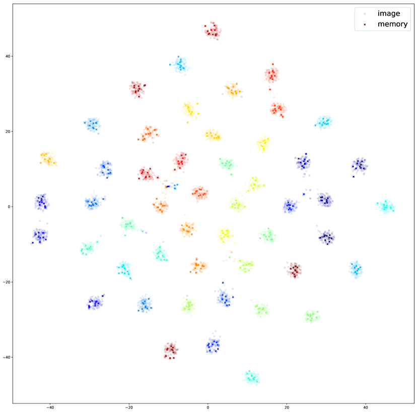
Figure 3: The t-SNE visualization for memory maintained in the setting of supervised learning. We randomly sample 50 out of 754 fine classes shown as different colors. The sampled image feature of the training samples and the stored memory feature for one class share the same color while the image feature has higher transparency. For each class, the image features surround the memory feature and features from different classes are dispersed from each other for classification.

6 Conclusion

In this paper, we study a new problem “many-class few-shot”(MCFS), which is a more challenging problem commonly encountered in practice compared to the previously studied “many-class many-shot”, “few-class few-shot” and “few-class many-shot” problems. We address the MCFS problem by training a multi-output model producing coarse-to-fine predictions, which leverages the class hierarchy information and explore the relationship between fine and coarse classes. We propose “Memory-Augmented Hierarchical-Classification Network (MahiNet)”, which integrates both MLP and learnable KNN classifiers with attention modules to produce reliable prediction of both the coarse and fine classes. In addition, we propose two new benchmark datasets with a class hierarchy structure and multi-label annotations for the MCFS problem, and show that MahiNet outperforms existing methods in both supervised learning and meta-learning settings on the benchmark datasets without losing advantages in efficiency.

Lu Liu received her bachelor’s degree from South China University of Technology (SCUT), Guangzhou, China, in 2017. She is currently pursuing the Ph.D. at the Center for Artificial Intelligence, University of Technology Sydney (UTS), Australia. Her current research interests include deep learning, machine learning, few-shot learning and meta-learning.

Tianyi Zhou is a Ph.D student of Paul G. Allen School of Computer Science and Engineering at University of Washington, Seattle. His research covers several topics of machine learning, natural language processing, statistics and data analysis. He has published 30+ papers at top conferences and journals including NeurIPS, ICML, ICLR, AISTATS, ACM SIGKDD, IEEE ICDM, AAAI, IJCAI, IEEE ISIT, Machine Learning Journal (Springer), DMKD (Springer), IEEE TIP, IEEE TNNLS, etc. He is the recipient of the best student paper award at IEEE ICDM 2013.

Guodong Long received his PhD degree from the University of Technology Sydney (UTS), Australia, in 2014. He is a senior lecturer at the Centre for Artificial Intelligence (CAI), Faculty of Engineering and IT, UTS. His research focuses on data mining, machine learning, and natural language processing. He has more than 40 research papers published on top-tier journals and conferences, including IEEE TPAMI, TCYB, TKDE, ICLR, AAAI, IJCAI, and ICDM.

Jing Jiang received her PhD degree from the University of Technology Sydney (UTS), Australia in 2015. She is currently a Lecturer at the Centre for Artificial Intelligence, Faculty of Engineering and IT, UTS. Her research interest lies in data mining and machine learning applications with the focuses on deep reinforcement learning and sequential decision-making. She has more than 20 research papers published on top-tier journals and conferences including AAAI, IJCAI and CCGrid.

Chengqi Zhang has been appointed as a Distinguished Professor at the University of Technology Sydney from 27 February 2017 to 26 February 2022, an Executive Director UTS Data Science from 3 January 2017 to 2 January 2021, an Honorary Professor at the University of Queensland from 1 January 2015 to 31 December 2017, an Adjunct Professor at the University of New South Wales from 20 March 2017 to 20 March 2020, and a Research Professor of Information Technology at UTS from 14 December 2001. In addition, he has been selected as the Chairman of the Australian Computer Society National Committee for Artificial Intelligence since November 2005, and the Chairman of IEEE Computer Society Technical Committee of Intelligent Informatics (TCII) since June 2014.

References

- [1] K. He, X. Zhang, S. Ren, and J. Sun, “Deep residual learning for image recognition,” in Proc. IEEE Conf. Comput. Vis. Pattern Recognit., 2016, pp. 770–778.
- [2] G. Huang, Z. Liu, L. Van Der Maaten, and K. Q. Weinberger, “Densely connected convolutional networks,” in Proc. IEEE Conf. Comput. Vis. Pattern Recognit., 2017, pp. 4700–4708.
- [3] M. Andrychowicz, M. Denil, S. Gómez, M. W. Hoffman, D. Pfau, T. Schaul, B. Shillingford, and N. de Freitas, “Learning to learn by gradient descent by gradient descent,” in Proc. Advances Neural Inf. Process. Syst., 2016, pp. 3981–3989.
- [4] K. Li and J. Malik, “Learning to optimize,” in Proc. Int. Conf. Learn. Representations, 2017.
- [5] S. Ravi and H. Larochelle, “Optimization as a model for few-shot learning,” in Proc. Int. Conf. Learn. Representations, 2017.
- [6] C. Finn, P. Abbeel, and S. Levine, “Model-agnostic meta-learning for fast adaptation of deep networks,” in Proc. Int. Conf. Machine Learning, 2017, pp. 1126–1135.
- [7] O. Vinyals, C. Blundell, T. Lillicrap, D. Wierstra et al., “Matching networks for one shot learning,” in Proc. Advances Neural Inf. Process. Syst., 2016, pp. 3630–3638.
- [8] J. Snell, K. Swersky, and R. Zemel, “Prototypical networks for few-shot learning,” in Proc. Advances Neural Inf. Process. Syst., 2017, pp. 4077–4087.
- [9] M. Douze, A. Szlam, B. Hariharan, and H. Jégou, “Low-shot learning with large-scale diffusion,” in Proc. IEEE Conf. Comput. Vis. Pattern Recognit., 2018, pp. 3349–3358.
- [10] J. Deng, W. Dong, R. Socher, L.-J. Li, K. Li, and L. Fei-Fei, “ImageNet: A large-scale hierarchical image database,” in Proc. IEEE Conf. Comput. Vis. Pattern Recognit., 2009, pp. 248–255.
- [11] B. Lake, R. Salakhutdinov, J. Gross, and J. Tenenbaum, “One shot learning of simple visual concepts,” in Proc. of the Annual Meeting of the Cognitive Science Society (CogSci), 2011, pp. 2568–2573.
- [12] F. S. Y. Yang, L. Zhang, T. Xiang, P. H. Torr, and T. M. Hospedales, “Learning to compare: Relation network for few-shot learning,” in Proc. IEEE Conf. Comput. Vis. Pattern Recognit., 2018, pp. 1199–1208.
- [13] L. Fei-Fei, R. Fergus, and P. Perona, “One-shot learning of object categories,” IEEE Trans. Pattern Anal. Mach. Intell., vol. 28, no. 4, pp. 594–611, 2006.
- [14] A. Wong and A. L. Yuille, “One shot learning via compositions of meaningful patches,” in Proc. IEEE Int. Conf. Comput. Vis., 2015, pp. 1197–1205.
- [15] B. M. Lake, R. R. Salakhutdinov, and J. Tenenbaum, “One-shot learning by inverting a compositional causal process,” in Proc. Advances Neural Inf. Process. Syst., 2013, pp. 2526–2534.
- [16] Y. Wang, R. Girshick, M. Hebert, and B. Hariharan, “Low-shot learning from imaginary data,” in Proc. IEEE Conf. Comput. Vis. Pattern Recognit., 2018, pp. 7278–7286.
- [17] D. K. Naik and R. Mammone, “Meta-neural networks that learn by learning,” in Proc. Int. Joint Conf. on Neural Networks, 1992, pp. 437–442.
- [18] J. Schmidhuber, “Evolutionary principles in self-referential learning, or on learning how to learn: the meta-meta-… hook,” Ph.D. dissertation, Institut f. Informatik, Tech. Univ. Munich, 1987.
- [19] P. Zhao, Y. Zhang, M. Wu, S. C. Hoi, M. Tan, and J. Huang, “Adaptive cost-sensitive online classification,” IEEE Trans. Knowl. Data Eng., vol. 31, no. 2, pp. 214–228, 2019.
- [20] B. M. Lake, R. Salakhutdinov, and J. B. Tenenbaum, “Human-level concept learning through probabilistic program induction,” Science, vol. 350, no. 6266, pp. 1332–1338, 2015.
- [21] G. Koch, R. Zemel, and R. Salakhutdinov, “Siamese neural networks for one-shot image recognition,” in Proc. Int. Conf. Machine Learning Workshop, 2015.
- [22] W. Yu, X. Lin, W. Zhang, J. Pei, and J. A. McCann, “Simrank*: effective and scalable pairwise similarity search based on graph topology,” The VLDB Journal, Jan 2019. [Online]. Available: https://doi.org/10.1007/s00778-018-0536-3
- [23] N. Mishra, M. Rohaninejad, X. Chen, and P. Abbeel, “A simple neural attentive meta-learner,” in Proc. Int. Conf. Learn. Representations, 2018.
- [24] L. Metz, N. Maheswaranathan, B. Cheung, and J. Sohl-Dickstein, “Learning unsupervised learning rules,” in Proc. Int. Conf. Learn. Representations, 2019.
- [25] J. Gu, Y. Wang, Y. Chen, K. Cho, and V. O. Li, “Meta-learning for low-resource neural machine translation,” in Conference on Empirical Methods in Natural Language Processing (EMNLP), 2018.
- [26] E. Schwartz, L. Karlinsky, J. Shtok, S. Harary, M. Marder, S. Pankanti, R. Feris, A. Kumar, R. Giries, and A. M. Bronstein, “Repmet: Representative-based metric learning for classification and one-shot object detection,” in Proc. IEEE Conf. Comput. Vis. Pattern Recognit., 2019.
- [27] K. R. Allen, E. Shelhamer, H. Shin, and J. B. Tenenbaum, “Infinite mixture prototypes for few-shot learning,” in Proc. Int. Conf. Machine Learning, 2019.
- [28] L. Liu, T. Zhou, G. Long, J. Jiang, L. Yao, and C. Zhang, “Prototype propagation networks (PPN) for weakly-supervised few-shot learning on category graph,” in Proc. Int. Joint Conf. on AI, 2019.
- [29] L. Liu, T. Zhou, G. Long, J. Jiang, and C. Zhang, “Learning to propagate for graph meta-learning,” in Proc. Advances Neural Inf. Process. Syst., 2019, pp. 1037–1048.
- [30] G. Tsoumakas and I. Katakis, “Multi-label classification: An overview,” International Journal of Data Warehousing and Mining (IJDWM), vol. 3, no. 3, pp. 1–13, 2007.
- [31] J. Read, B. Pfahringer, G. Holmes, and E. Frank, “Classifier chains for multi-label classification,” in Joint European Conference on Machine Learning and Knowledge Discovery in Databases. Springer, 2009, pp. 254–269.
- [32] J. Read, L. Martino, and D. Luengo, “Efficient monte carlo methods for multi-dimensional learning with classifier chains,” Pattern Recognition, vol. 47, no. 3, pp. 1535–1546, 2014.
- [33] J. Read, L. Martino, P. M. Olmos, and D. Luengo, “Scalable multi-output label prediction: From classifier chains to classifier trellises,” Pattern Recognition, vol. 48, no. 6, pp. 2096–2109, 2015.
- [34] N. SpolaôR, E. A. Cherman, M. C. Monard, and H. D. Lee, “A comparison of multi-label feature selection methods using the problem transformation approach,” Electronic Notes in Theoretical Computer Science, vol. 292, pp. 135–151, 2013.
- [35] W. Liu, D. Xu, I. Tsang, and W. Zhang, “Metric learning for multi-output tasks,” IEEE Trans. Pattern Anal. Mach. Intell., vol. 41, no. 2, pp. 408–422, 2019.
- [36] W. Liu and I. W. Tsang, “Making decision trees feasible in ultrahigh feature and label dimensions,” Journal of Machine Learning Research, vol. 18, no. 1, pp. 2814–2849, 2017.
- [37] J. Read, B. Pfahringer, and G. Holmes, “Multi-label classification using ensembles of pruned sets,” in Proc. IEEE Int. Conf. on Data Mining. IEEE, 2008, pp. 995–1000.
- [38] G. Tsoumakas, I. Katakis, and I. Vlahavas, “Mining multi-label data,” in Data mining and knowledge discovery handbook. Springer, 2009, pp. 667–685.
- [39] S. Li, Y. Jiang, N. V. Chawla, and Z. Zhou, “Multi-label learning from crowds,” IEEE Trans. Knowl. Data Eng., vol. 31, no. 7, pp. 1369–1382, July 2019.
- [40] D. Heider, R. Senge, W. Cheng, and E. Hüllermeier, “Multilabel classification for exploiting cross-resistance information in hiv-1 drug resistance prediction,” Bioinformatics, vol. 29, no. 16, pp. 1946–1952, 2013.
- [41] C. N. Silla and A. A. Freitas, “A survey of hierarchical classification across different application domains,” Data Mining and Knowledge Discovery, vol. 22, no. 1-2, pp. 31–72, 2011.
- [42] A. D. Gordon, “A review of hierarchical classification,” Journal of the Royal Statistical Society: Series A (General), vol. 150, no. 2, pp. 119–137, 1987.
- [43] J. Wehrmann, R. Cerri, and R. Barros, “Hierarchical multi-label classification networks,” in Proc. Int. Conf. Machine Learning, 2018, pp. 5225–5234.
- [44] S. Dumais and H. Chen, “Hierarchical classification of web content,” in Proceedings of the International ACM SIGIR conference on Research and development in Information Retrieval. ACM, 2000, pp. 256–263.
- [45] A. Sun and E.-P. Lim, “Hierarchical text classification and evaluation,” in Proc. IEEE Int. Conf. on Data Mining. IEEE, 2001, pp. 521–528.
- [46] H. G. Gauch Jr and R. H. Whittaker, “Hierarchical classification of community data,” The Journal of Ecology, pp. 537–557, 1981.
- [47] Q. Zhang, C. Shi, Z. Niu, and L. Cao, “Hcbc: A hierarchical case-based classifier integrated with conceptual clustering,” IEEE Trans. Knowl. Data Eng., vol. 31, no. 1, pp. 152–165, Jan 2019.
- [48] Y. Yang, Y. Duan, X. Wang, Z. Huang, N. Xie, and H. T. Shen, “Hierarchical multi-clue modelling for poi popularity prediction with heterogeneous tourist information,” IEEE Trans. Knowl. Data Eng., vol. 31, no. 4, pp. 757–768, 2019.
- [49] B. Lyu, L. Qin, X. Lin, L. Chang, and J. X. Yu, “Supergraph search in graph databases via hierarchical feature-tree,” IEEE Trans. Knowl. Data Eng., vol. 31, no. 2, pp. 385–400, 2019.
- [50] D. Ouyang, L. Qin, L. Chang, X. Lin, Y. Zhang, and Q. Zhu, “When hierarchy meets 2-hop-labeling: Efficient shortest distance queries on road networks,” in Proceedings of the 2018 International Conference on Management of Data, ser. SIGMOD ’18. New York, NY, USA: ACM, 2018, pp. 709–724. [Online]. Available: http://doi.acm.org/10.1145/3183713.3196913
- [51] M. Ren, E. Triantafillou, S. Ravi, J. Snell, K. Swersky, J. B. Tenenbaum, H. Larochelle, and R. S. Zemel, “Meta-learning for semi-supervised few-shot classification,” in Proc. Int. Conf. Learn. Representations, 2018.
- [52] A. Li, T. Luo, Z. Lu, T. Xiang, and L. Wang, “Large-scale few-shot learning: Knowledge transfer with class hierarchy,” in Proceedings of the IEEE Conference on Computer Vision and Pattern Recognition, 2019, pp. 7212–7220.
- [53] H. Yao, Y. Wei, J. Huang, and Z. Li, “Hierarchically structured meta-learning,” 2019.
- [54] G. Valentini, “True path rule hierarchical ensembles for genome-wide gene function prediction,” IEEE/ACM Transactions on Computational Biology and Bioinformatics (TCBB), vol. 8, no. 3, pp. 832–847, 2011.
- [55] N. Cesa-Bianchi, M. Re, and G. Valentini, “Synergy of multi-label hierarchical ensembles, data fusion, and cost-sensitive methods for gene functional inference,” Machine Learning, vol. 88, no. 1-2, pp. 209–241, 2012.
- [56] G. Yu, H. Zhu, C. Domeniconi, and J. Liu, “Predicting protein function via downward random walks on a gene ontology,” BMC bioinformatics, vol. 16, no. 1, p. 271, 2015.
- [57] G. Yu, G. Fu, J. Wang, and Y. Zhao, “Newgoa: Predicting new go annotations of proteins by bi-random walks on a hybrid graph,” IEEE/ACM Transactions on Computational Biology and Bioinformatics (TCBB), vol. 15, no. 4, pp. 1390–1402, 2018.
- [58] B. Gholami and V. Pavlovic, “Probabilistic temporal subspace clustering,” in Proc. IEEE Conf. Comput. Vis. Pattern Recognit., 2017, pp. 3066–3075.
- [59] A. Vaswani, N. Shazeer, N. Parmar, J. Uszkoreit, L. Jones, A. N. Gomez, Ł. Kaiser, and I. Polosukhin, “Attention is all you need,” in Proc. Advances Neural Inf. Process. Syst., 2017, pp. 5998–6008.
- [60] A. A. Rusu, D. Rao, J. Sygnowski, O. Vinyals, R. Pascanu, S. Osindero, and R. Hadsell, “Meta-learning with latent embedding optimization,” in Proc. Int. Conf. Learn. Representations, 2018.
- [61] A. Nichol, J. Achiam, and J. Schulman, “On first-order meta-learning algorithms,” arXiv preprint arXiv:1803.02999, 2018.
- [62] Y. Wu and K. He, “Group normalization,” in Proc. Eur. Conf. Comput. Vis., 2018, pp. 3–19.
- [63] S. Ioffe and C. Szegedy, “Batch normalization: Accelerating deep network training by reducing internal covariate shift,” in Proc. Int. Conf. Machine Learning, 2015, pp. 448–456.
- [64] D. P. Kingma and J. Ba, “Adam: A method for stochastic optimization,” in Proc. Int. Conf. Learn. Representations, 2015.
- [65] A. Santoro, S. Bartunov, M. Botvinick, D. Wierstra, and T. Lillicrap, “Meta-learning with memory-augmented neural networks,” in Proc. Int. Conf. Machine Learning, 2016, pp. 1842–1850.
- [66] L. v. d. Maaten and G. Hinton, “Visualizing data using t-sne,” Journal of Machine Learning Research, vol. 9, no. 11, pp. 2579–2605, 2008.