An effective 2D model for MHD flows with transverse magnetic field

Abstract

This paper presents a model for quasi two-dimensional MHD flows between two planes with small magnetic Reynolds number and constant transverse magnetic field orthogonal to the planes. A method is presented that allows to take 3D effects into account in a 2D equation of motion thanks to a model for the transverse velocity profile. The latter is obtained by using a double perturbation asymptotic development both in the core flow and in the Hartmann layers arising along the planes. A new model is thus built that describes inertial effects in these two regions. Two separate classes of phenomena are thus pointed out : the one related to inertial effects in the Hartmann layer gives a model for recirculating flows and the other introduces the possibility of having a transverse dependence of the velocity profile in the core flow. The ”recirculating” velocity profile is then introduced in the transversally averaged equation of motion in order to provide an effective 2D equation of motion. Analytical solutions of this model are obtained for two experimental configurations : isolated vortices aroused by a point electrode and axisymmetric parallel layers occurring in the MATUR (MAgneticTURbulence) experiment. The theory is found to give a satisfactory agreement with the experiment so that it can be concluded that recirculating flows are actually responsible for both vortices core spreading and excessive dissipative behavior of the axisymmetric side wall layers.

1 Introduction.

Magnetohydrodynamic flows at the laboratory scale have been the subject of many investigations during the last decades, which lead to a rather good level of understanding (see, for instance Hunt and Shercliff (1971) and Moreau (1990)). In this paper, we focus on flows of incompressible fluids, such as liquid metals, in the presence of a uniform magnetic field $\mathbf{B}$. The magnetic Reynolds number $Rm=\mu\sigma UL$ ($\mu$ denotes the fluid magnetic permeability, $\sigma$ its electrical conductivity, $U$ and $L$ are typical velocity and length scales) is supposed significantly smaller than unity, so that the actual magnetic field within the fluid is close to $\mathbf{B}$. The fluid flows in a container bounded by two insulating walls perpendicular to the magnetic field (usually named Hartmann Walls ). Nothing is specified for the other boundaries (for instance the wall parallel to the magnetic field) or for the driving mechanisms (except when particular examples are considered). The magnetic field is supposed high enough, so that both the Hartmann number ($Ha=aB\sqrt{\sigma/\rho\nu}$) and the interaction parameter ($N=\sigma B^{2}a/\rho U$) are much larger than unity (here $a$ is the distance separating the two Hartmann walls, $\rho$ the fluid density and $\nu$ its kinematic viscosity). In such flows, the Hartmann boundary layers which develop along the Hartmann walls are of primary importance.

One of the most important features of these flows is the fact that turbulence is only weakly damped out by the electromagnetic force. Indeed, because of their tendency to form quasi-two-dimensional (2D) structures, these flows induce a significant current density only within the Hartmann layers whose thickness is of the order $Ha^{-1}$. As a consequence the quasi-2D core is only weakly affected by Joule dissipation and a highly energetic turbulence may be observed (Lielausis (1975) ). In such a configuration, the persistence of two-dimensional turbulence and its specific properties have been found by Kolesnikov and Tsinober (1974) in decaying grid turbulence and then by Sommeria (1986) in electromagnetically forced regimes.

To understand this persistence of turbulence and its quasi-two-dimensionality the reader is referred to a number of earlier papers. In particular, Alemany et al.(1979) demonstrated how an initially isotropic grid turbulence develops an increasing anisotropy. However in this experiment, because there is no confinement by Hartmann walls, the ohmic damping is of primary importance: the characteristic time for both the development of the anisotropy and the ohmic damping is $\rho/\sigma B^{2}$ and may be shorter than the eddy turnover time. The key mechanisms are explained in Sommeria and Moreau (1982) and in a review paper (Moreau 1998). More recently, Davidson (1997) pointed out the crucial role of the invariance of the component of the angular momentum parallel to the magnetic field (whereas the components perpendicular to $\mathbf{B}$ decrease on the timescale $\rho/\sigma B^{2}$) and Ziganov and Thess (1998) achieved a numerical simulation of this phenomenon exhibiting the sequences of events which lead to the formation of column-like turbulent structures elongated in the direction of the magnetic field. But these two theoretical approaches, as well as the experimental part of Alemany et al.(1979), which do not involve the confinement by Hartmann walls, are not directly relevant for the quasi-2D flows considered here.

In this case, Sommeria and Moreau (1982) have described how the magnetic field tends to suppress velocity differences in transverse planes. If the Hartmann number and interaction parameter are sufficiently large, this phenomenon can be considered as instantaneous so that the flow is not dependent on the space coordinate associated with the field direction anymore, except in Hartmann layers, where the velocity exhibits an exponential profile given by the classical Hartmann layer theory. Integrating the equation of motion along the field direction then provides a 2D Navier-Stokes equation with a forcing and a linear braking representing electromagnetic effects and friction in the Hartmann layers. This ”2D core model” has provided a good quantitative prediction for various electromagnetically driven flows (Sommeria, 1988). It has been generalized by Bühler (1996) to account for the presence of walls with various conductivities, and applied to configurations of interest for the design of lithium blankets in nuclear fusion reactors.

However, this 2D core model is only justified for $N$ and $Ha$ much larger than unity, and discrepancies with experiments have been observed for moderate values of the interaction parameter $N$. Then Ekman recirculating flows are produced by inertial effects in the Hartmann layer. As a consequence, a spreading of the vortex core was observed by Sommeria (1988) for vortices aroused by a point electrode. Such inertial effects have been more systematically investigated in recent experiments of electrically driven circular flows (Alboussière et al 1999 ). In the inertialess limit, complete 3D calculations provide linear solutions for such flows or for parallel layers, but no analytical model describes their non linear behavior due to inertial effects.

The present work aims at building such a model by a systematic expansion in terms of the small parameters $Ha^{-1}$ and $N^{-1}$. The 2D core model of Sommeria & Moreau (1982) is recovered at the leading order, and three-dimensional effects arise as perturbations.

In the next section we first recall the complete 3D equations. The electromagnetic effects are interpreted as a diffusion of momentum along the magnetic field direction, which tends to soften velocity differences between transverse planes, thus driving the flow toward a 2D state in the core. We also derive a 2D evolution equation for quantities averaged across the fluid layer along the magnetic field direction (which we shall suppose ”vertical” to simplify the description). This vertically averaged 2D equation is always valid, even when the 2D core structure is not reached, but it then involves terms depending on the vertical velocity profile, similar to usual Reynolds stresses. For a 2D core with Hartmann boundary layers, this vertically averaged equation reduces to the 2D core model of Sommeria & Moreau (1982), that we recall in section 2.2. We stress that it can be applied even in the parallel boundary layers near the lateral walls, or in the core of a vortex electromagnetically driven around a point electrode (scaling as $aHa^{-1/2}$ like parallel boundary layers). Indeed the 2D core model compares well with linear theories involving a complete 3D calculation.

Section 3 is devoted to the detailed investigation of the complete 3D equations, using a double perturbation method simultaneously in the core and in the Hartmann layer. A first kind of 3D effects, discussed in section 3.2, is the presence of recirculating flows driven by inertial effects in the Hartmann layer. For axisymmetric flows, this is an Ekman pumping mechanism. A second kind of 3D effect, occurring in the core, is discussed in section 3.3 : a perturbation of the 2D core, with a profile quadratic in the vertical coordinate, is due to the finite time of action of the electromagnetic diffusion of momentum along the vertical direction. Thus in unsteady regimes, vortices are ”barrel” shaped, instead of truly columnar. Introducing some of these perturbations of the vertical velocity profile in the vertically averaged equations yields an effective 2D model, described in section 3.4. This is the main result of the present paper. The new terms involved in this model are mostly important for small horizontal scales, leading in particular to new kinds of parallel layers near curved walls or in the core of vortices, as specifically discussed in section 3.5.

This effective 2D model could be implemented in numerical computations of various MHD flows between two Hartmann walls (or with a bottom wall and a quasi-horizontal free surface). We discuss in section 4 the application to axisymmetric flows. We apply the results to the electromagnetically generated vortex of Sommeria (1988) and to the MATUR experiments (Alboussière et al. 1999). The discrepancies of the 2D core model are reasonably accounted by our effective 2D model, taking into account the influence of recirculating flows.

2 General equations and 2D-core model.

2.1 General equations and z-averaging

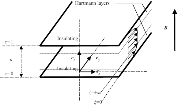
Figure 1: Geometric configuration considered in our model.

The fluid of density $\rho$, kinematic viscosity $\nu$ and electrical conductivity $\sigma$ is supposed to flow between two electrically insulating plates orthogonal to the uniform magnetic field $\mathbf{B}$ (see figure 1). We suppose $\mathbf{B}$ is vertical for the simplicity of description (although there is no gravity effect). We start from the Navier-Stokes equations for an incompressible fluid with a priori 3D velocity field $\mathbf{u}$ and pressure $p$. The non-dimensional variables and coordinates are defined from physical variables (labelled by the subscript ()_dimas

$$\begin{array}[]{cccc}x_{dim}=\dfrac{a}{\lambda}x&t_{dim}=\dfrac{a}{\lambda U}t&\mathbf{j}_{\bot dim}\mathbf{=}\sigma BU\mathbf{j}&p_{dim}=\rho U^{2}p\\ y_{dim}=\dfrac{a}{\lambda}y&\mathbf{u_{\perp}}_{dim}\mathbf{=}U\mathbf{u_{\perp}}&j_{zdim}\mathbf{=}\lambda\sigma BUj_{z}&\mathbf{B}_{dim}\mathbf{=}B\mathbf{e}_{z}\\ z_{dim}=az&w_{dim}=\lambda Uw&&\end{array}$$ (1)

Note that we distinguish the scales parallel and perpendicular (with the aspect ratio $\lambda$) to the magnetic field, and the corresponding velocities ($\mathbf{u_{\perp},}w$) and currents ($\mathbf{j}_{\bot},j_{z}$) accordingly. The subscript $\bot$ denotes the vector projection in the direction perpendicular to the magnetic field. The Hartmann number $Ha$ and the interaction parameter $N$ are defined as :

$$\begin{array}[]{cc}Ha=aB\sqrt{\dfrac{\sigma}{\rho\nu}},&N=\dfrac{\sigma B^{2}a}{\rho U}\end{array}.$$ (2)

Notice that the Reynolds number is defined as $Re=Ha^{2}/N$. It may be noticed that all these non-dimensional numbers are built with the layer thickness $a$.

Using these dimensionless variables, the motion equations write

$$\mathbf{\nabla}_{\perp}.\mathbf{u_{\perp}+}\partial_{z}w = 0\text{,}$$ (3)

$$\dfrac{\lambda}{N}\left(\partial_{t}\mathbf{u_{\perp}}+\mathbf{u_{\perp}.\nabla}_{\perp}\mathbf{u_{\perp}}+w\partial_{z}\mathbf{u_{\perp}}+\nabla_{\perp}p\right)-\dfrac{\lambda^{2}}{Ha^{2}}\Delta_{\perp}\mathbf{u_{\perp}-}\dfrac{1}{Ha^{2}}\partial_{zz}^{2}\mathbf{u_{\perp}} = \mathbf{j}_{\bot}\times\mathbf{e}_{z},$$ (4)

$$\dfrac{\lambda}{N}\left(\partial_{t}w+\mathbf{u_{\perp}.\nabla}_{\perp}w+w\partial_{z}w+\partial_{z}p\right)-\dfrac{\lambda^{2}}{Ha^{2}}\Delta_{\perp}w\mathbf{-}\dfrac{1}{Ha^{2}}\partial_{zz}^{2}w = 0,$$ (5)

$$\mathbf{\nabla}_{\perp}.\mathbf{j}_{\bot}+\partial_{z}j_{z}=0,$$ (6)

$$\mathbf{j}=-\mathbf{\nabla}\phi+\mathbf{u}\times\mathbf{e}_{z}.$$ (7)

The electromagnetic force $\mathbf{j}\times\mathbf{e}_{z}$ has been included, where the electric current density $\mathbf{j}$ is related to the electric potential $\phi$ by (7), representing Ohm’s law. As the action of the induced magnetic field is negligible, the electromagnetic equations reduce to the condition of divergence-free current (6).

The electromagnetic force depends linearly on the velocity field, but in a non-local way. The current density $\mathbf{j}$ can be eliminated in (4) (see for example Roberts (1967) ). Denoting $\mathbf{j}\times\mathbf{e}_{z}\mathbf{=f+\nabla}p_{\varepsilon}$ in order to distinguish the rotational part and the divergent part of the Lorentz force, taking twice the curl of $\mathbf{j}\times\mathbf{e}_{z}$ and using (6) and (7) yields :

$$\Delta\mathbf{f}=\partial_{zz}^{2}\mathbf{u,}$$ (8)

Note that $p_{\varepsilon}$ can be included in the pressure term. In the limit of strong magnetic field, the force becomes very large, resulting in a fast damping by Joule effect, except if $\partial_{zz}^{2}\mathbf{u}$ is small, i.e. the flow is close to two-dimensional. In this case, $\Delta\mathbf{f\simeq}\Delta_{{}_{\bot}}\mathbf{f}$ , where $\Delta_{{}_{\bot}}$ stands for the Laplacian in the plane perpendicular to the magnetic field. Sommeria & Moreau (1982) proposed to interpret this force as a momentum diffusion along the direction of the magnetic field, with a ”diffusivity” $\tfrac{\sigma B^{2}a^{2}}{\lambda^{2}\rho}$ depending on the transverse scale $a/\lambda$. This diffusion tends to achieve two-dimensionality in the fluid interior when the corresponding diffusion time is smaller than the eddy turnover time $\tfrac{a}{\lambda U},$ i.e.:

$$\dfrac{\rho}{\sigma B^{2}}\lambda^{2}<<\dfrac{a}{\lambda U}\text{{i.e }}\lambda^{3}<<N,$$ (9)

However in order to take into account weak 3D effects, we shall not assume two-dimensionality right away, but get a 2D model by integrating the 3D equations along the direction of the magnetic field (i.e. the $z$ coordinate), leading to a 2D dynamics for z-averaged quantities. We define the z-average of any quantity $g$ and its departure from average $g\prime$ respectively by

$$\begin{array}[]{cc}\bar{g}(x,y)=\int_{0}^{1}gdz,&g^{\prime}(x,y,z)=g-\bar{g}\end{array}.$$ (10)

The z–average of the momentum equation (4) then leads to

$$\dfrac{\lambda}{N}\left(\partial_{t}\mathbf{\bar{u}}_{\bot}+\left(\mathbf{\bar{u}}_{\bot}\mathbf{.\nabla}\right)\mathbf{\bar{u}}_{\bot}\mathbf{+}\overline{\left(\mathbf{u}_{\bot}^{\prime}\mathbf{.\nabla}\right)\mathbf{u}_{\bot}^{\prime}}+\mathbf{\nabla}\overline{p}\right)=\dfrac{\lambda^{2}}{Ha^{2}}\mathbf{\Delta\bar{u}}_{\bot}+\dfrac{1}{Ha^{2}}\mathbf{\tau}_{W}+\overline{\mathbf{j}}\mathbf{\times e}_{z}$$ (11)

for each velocity component $\mathbf{u}_{\bot}$ ($j\in\left\{1,2\right\}$) perpendicular to the magnetic field. Here $\mathbf{\tau}_{W}=-[\partial_{z}\mathbf{u}_{\bot}$ $(z=0)-\partial_{z}\mathbf{u}_{\bot}(z=a)]$ denotes the sum of the non-dimensional viscous stresses at the lower and upper walls. The z-average of the continuity equation (3), with the impermeability conditions at the walls, indicates that the z-averaged velocity is divergence free in two dimensions. Therefore the initial 3D problem translates into a problem of an incompressible flow $\mathbf{\bar{u}}_{\bot}$ satisfying the 2D Navier-Stokes equation with two added terms : the divergence of a Reynolds stress tensor $\underline{\underline{\mathbf{\nabla}}}.\overline{\mathbf{u}_{\bot}^{\prime t}\mathbf{u}_{\bot}^{\prime}}$, resulting from the momentum transport by the 3D flow component, and the wall friction term $\mathbf{\tau}_{W}.$ The knowledge of both terms requires a model for the vertical velocity profile whose derivation is the main issue of section 3.

The electromagnetic term $\overline{\mathbf{j}}\mathbf{\times e}_{z}$ can be expressed from the current density $j_{W}$ $(x,y)$ injected in the fluid through the two walls (at $z=0$ and $z=1$). Indeed, the z-average of (6) yields $\mathbf{\nabla}_{\bot}.\overline{\mathbf{j}_{\bot}}=j_{W}$, and the z-average of (7) yields $\mathbf{\nabla}_{\bot}\times\overline{\mathbf{j}_{\bot}}=0$  (using the incompressibility condition $\mathbf{\nabla}_{\bot}.\mathbf{\bar{u}}_{\bot}=0$). Thus the z-averaged current can be expressed as the gradient of a scalar $\Psi_{0}$ satisfying a Poisson equation,

$$\begin{array}[]{cc}\overline{\mathbf{j}_{\bot}}=\dfrac{1}{Ha}\mathbf{\nabla}\Psi_{0},&\dfrac{1}{Ha}\Delta_{\bot}\Psi_{0}=-j_{W}\end{array}.$$ (12)

We shall consider either the case of insulating walls or the case of a current density imposed on electrodes (in more complex cases of conducting Hartmann walls, $j_{W}$ would be determined by a matching with Ohm’s law in the conductor). The boundary conditions on the side walls for $\Psi_{0}$ depend on the electrical condition : for electrically insulating lateral walls (supposed tangent to the magnetic field), there is no normal current, so that the normal derivative of $\Psi_{0}$ vanishes (Neuman conditions). By contrast, for a perfectly conducting lateral wall , the current is normal, so that $\Psi_{0}$ is constant on the wall (Dirichlet conditions)

Using (12), the electromagnetic force $\overline{\mathbf{j}}\mathbf{\times e}_{z}$ in (11) can be expressed as a divergence-free horizontal vector, and the 2D equation of motion writes :

$$\dfrac{\lambda}{N}\left(\partial_{t}\mathbf{\bar{u}}_{\bot}+\left(\mathbf{\bar{u}}_{\bot}\mathbf{.\nabla}\right)\mathbf{\bar{u}}_{\bot}\mathbf{+}\overline{\left(\mathbf{u}^{\prime}\mathbf{.\nabla}\right)\mathbf{u}^{\prime}}+\mathbf{\nabla}\overline{p}\right)=\dfrac{\lambda^{2}}{Ha^{2}}\mathbf{\Delta}_{\bot}\mathbf{\bar{u}}_{\bot}+\dfrac{1}{Ha^{2}}\mathbf{\tau}_{W}+\dfrac{1}{Ha}\mathbf{u}_{0},$$ (13)

where the 2D velocity field$\ \mathbf{u}_{0}\mathbf{\ }$is defined as $\mathbf{u}_{0}=\mathbf{\nabla}\Psi_{0}\times\mathbf{e}_{z}$.

2.2 The 2D core model.

2.2.1 The Hartmann friction

In the boundary layers, the z-derivatives dominate in (3-7), resulting in the Hartmann velocity profile, near the wall $z=0$

$$\mathbf{u}_{\perp}=\mathbf{u}^{-}\left(1-e^{-Ha\text{ }z}\right),$$ (14)

where $\mathbf{u}^{-}$ is the horizontal velocity near the wall, but outside the boundary layer. The corresponding wall stress is :

$$\mathbf{\tau}^{-}=-Ha\text{ }\mathbf{u}^{-}.$$ (15)

At the wall $z=a$ we shall consider either a free surface, supposed horizontal, with no stress, either a solid wall, with corresponding velocity $\mathbf{u}^{+}$ and wall stress $\mathbf{\tau}^{+}.$

We consider for the moment a 2D core velocity, so that $\mathbf{u}^{\mathbf{+}}=\mathbf{u}^{\mathbf{-}}\simeq\overline{\mathbf{u}}$ (neglecting the velocity fall in the boundary layer, as the latter is thin ($a/Ha)$ compared with the total thickness $a$). This wall stress introduces a global linear braking with characteristic time (for one Hartmann layer)

$$t_{H}=\dfrac{a^{2}}{\nu}\dfrac{1}{Ha}$$ (16)

and the 2D core velocity field satisfies in non-dimensional form :

$$\dfrac{\lambda}{N}\left[(\partial_{t}+\mathbf{\bar{u}}_{\bot}.\mathbf{\nabla})\mathbf{\bar{u}}_{\bot}+\mathbf{\nabla}\bar{p}\right]=\dfrac{\lambda^{2}}{Ha^{2}}\mathbf{\Delta\bar{u}}_{\bot}+\dfrac{1}{Ha}\left(\mathbf{u}_{0}-n\mathbf{\bar{u}}_{\bot}\right),$$ (17)

where $n$ is the number of Hartmann walls ($n=1$ in the case with a free surface and $n=2$ for a flow between two Hartmann walls, such that the friction is doubled).

The whole model was discussed by Sommeria and Moreau (1982) and applied to various cases. It applies for sufficiently large perpendicular scales $\dfrac{a}{\lambda}$, such that condition (9) is satisfied. In principle it should break down in the parallel boundary layers, of thickness $\mathcal{O}(aHa^{-1/2})$, but it is interesting to test its validity in this case. We shall consider two cases for which a three-dimensional analytical solution is available as a reference: the parallel side boundary layer and an isolated vortex aroused by a point-electrode.

2.2.2 Sidewall layers

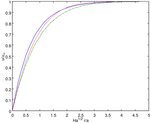
Figure 2: Comparison between the 1D profile (16) (solid line) and the corresponding profile for the 2D averaged solution of Shercliff (1953) : the dotted line represents the profile at $z=1/2$ and the dashed line, the z average profile.

Let us consider the case of a duct flow with rectangular section, as first solved by Shercliff (1953). In this case, the flow is driven by pressure drop, which can be modelled with a uniform forcing velocity $\mathbf{u}_{0}$ (like in the case of a uniform electromagnetic driving by a transverse current). Then, equation (17) reduces to

$$\dfrac{\lambda^{2}}{Ha}\partial_{yy}\bar{u}_{x}\left(y\right)-\left(2\bar{u}_{x}\left(y\right)-u_{0x}\right)=0,$$ (18)

the solution of which is, near the side wall supposed located at $y=0$ :

$$\dfrac{\bar{u}\left(y\right)}{u_{0x}}=1-\exp\left(-y\dfrac{\sqrt{2Ha}}{\lambda}\right).$$ (19)

Notice that this side boundary layer has a thickness $\tfrac{a}{\lambda}\simeq\tfrac{a}{\sqrt{Ha}}$ which results from a balance between lateral diffusion, with time scale $\tfrac{a^{2}}{\lambda^{2}\nu}$, and the Hartmann friction with time scale $t_{H}$ ($\tfrac{a}{\lambda}\simeq\sqrt{\nu t_{H}}$). The velocity profile is plotted in figure (2) and compared with the 3D solution (see for instance Moreau (1990)).   Both the velocity in the middle plane ($z=1/2$) and the z-averaged velocity are found in reasonable agreement with the 2D core model although the hypotheses the latter relies on are not fully satisfied in these side boundary layers. The profiles of figure (4) confirm that the 3D solution is not very far for from a 2D core. Notice that the electric condition at the parallel wall is not of great importance since it only induces a variation of a few percents on the velocity. By contrast, the Hartman wall has to be insulating as discussed in section 3.1 : indeed, with conducting walls , there would be strong jets in the parallel layer which cannot be described by this model.

2.2.3 Isolated vortices

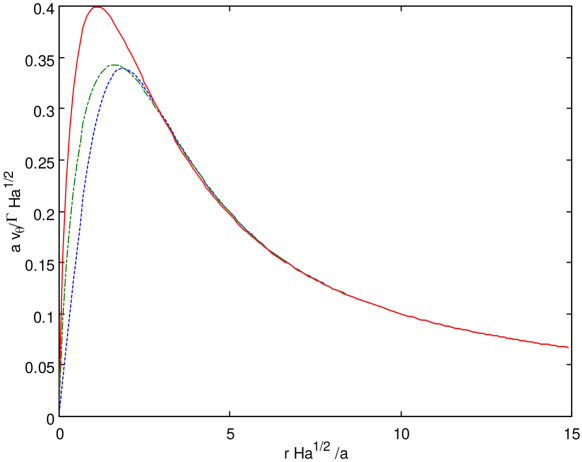
Figure 3: Comparison between the 1D velocity profile (18) (solid line) and the 2D solution of Sommeria (1988) for an electrically driven vortex. The dotted line represents the profile at $z=1/2$ and the dashed line, the average profile.

Here, the 2D model is used to compute the velocity profile for an isolated vortex driven by the electric current injected at a point electrode located in the bottom plate, experimentally studied by Sommeria (1988). The upper surface is free (but remaining quasi-horizontal) and side walls are supposed very far. Therefore the source term $j_{W}$ in (12) is a Dirac function with integral equal to the injected current $I$, and the corresponding forcing  $\mathbf{u}_{0}$ is azimuthal and depends on the radius $r$ as

$$u_{0\theta}=\dfrac{\Gamma}{r}\text{\ avec }\Gamma=\dfrac{I}{2\pi\sqrt{\rho\sigma\nu}},$$ (20)

where the velocity and the space coordinate have been rescaled using $U=\tfrac{\Gamma\sqrt{Ha}}{a}$ and $\lambda=\sqrt{Ha}$ (which corresponds to the non-dimensional parallel layer thickness). The radial velocity profile then results from the balance between electric forcing , Hartmann braking, and lateral viscous stress. A steady laminar and axisymmetric solution of (17) in polar coordinates is given by

$$u_{\theta}=\dfrac{1}{\tilde{r}}-K_{1}\left(\tilde{r}\right),$$ (21)

where $K_{1}$ denotes the modified Bessel function of the second kind. Hunt and Williams (1968) have performed a complete asymptotic three-dimensional resolution of an analogous problem for large values of the Hartmann number. The latter can be adapted to the present case through simple transformations (Sommeria 1988) :

$$v_{\theta}=\dfrac{1}{r}\left(1-\dfrac{1}{2}\exp\left(\dfrac{-r^{2}}{4z}\right)-\dfrac{1}{2}\exp\left(\dfrac{-r^{2}}{4\left(2-z\right)}\right)\right).$$ (22)

As in the previous sub-section, we compare the value of this solution at the middle plane ($z=1/2$) and its z-average to the 2D solution (21)(see figure 3). A reasonable agreement between 2D and 3D theories is obtained, in spite of the very singular behavior of the 3D solution near the electrode. It is interesting to notice that the simplified 2D theory gives the right orders of magnitude for the core diameter and the maximum velocity as well.

3 An effective quasi 2-D model.

3.1 Non-dimensional basic equations.

In this section the modifications of the Hartmann profile (14) are derived by a perturbation method. Let us first replace equation (7) by its curl $\mathbf{\nabla\times j}=\left(\mathbf{e}_{z}.\mathbf{\nabla}\right)\mathbf{u}$ in order to express the electromagnetic effects directly in terms of the velocity field. Distinguishing the transverse and parallel components of $\mathbf{\nabla\times j,}$ we get the equations for $\mathbf{j}$ :

$$\mathbf{\nabla}_{\bot}\mathbf{\times j}_{\bot} = \partial_{z}w,$$ (23)

$$\mathbf{e}_{z}\times\partial_{z}\mathbf{j}_{\bot}-\lambda^{2}\left(\mathbf{e}_{z}\times\mathbf{\nabla}_{\perp}\right)j_{z} = \partial_{z}\mathbf{u_{\perp}.}$$ (24)

We could deduce from these three equations the equation for the force $\mathbf{j}_{\bot}\times\mathbf{e}_{z}$ (the non dimensional form of (8)), but the information on the boundary condition for $j_{z}$ would be lost.

In the Hartmann boundary layer, the $z$ coordinate scales like the Hartmann layer thickness $a/Ha$. We use the subscript $(\ )_{h}$ to denote the variables within the boundary layer which are functions of the argument$\ \xi$ $=Ha$ $z$ , the stretched $z$ coordinate ($\mathbf{u}_{h}$ and $w_{h}$ denote the velocity components perpendicular and parallel to the magnetic field, respectively, whereas $\mathbf{j}_{h}$ and $j_{\xi}$ stand for the horizontal and vertical electric current density). Then, equations (23) and (24) become :

$$\dfrac{1}{Ha}\mathbf{\nabla}_{\perp}\times\mathbf{j}_{h}=\partial_{\xi}w_{h},$$ (25)

$$-\dfrac{\lambda^{2}}{Ha}\left(\mathbf{e}_{z}\times\mathbf{\nabla}_{\bot}\right)j_{\xi}=-\mathbf{e}_{z}\times\partial_{\xi}\mathbf{j}_{h}+\partial_{\xi}\mathbf{u}_{h}.$$ (26)

They have to be completed by the condition of conservation of electric current (6) which becomes within the Hartmann layer :

$$\dfrac{1}{Ha}\mathbf{\nabla}_{\perp}.\mathbf{j}_{h}=-\partial_{\xi}j_{\xi}.$$ (27)

With the same transformation, the equation of motion (3-4) become :

$$\xi=Ha\text{ }z$$ (28)

$$\dfrac{1}{Ha}\mathbf{\nabla}_{\perp}.\mathbf{u}_{h} = \partial_{\xi}w_{h},$$ (29)

$$\dfrac{\lambda}{N}\left(\partial_{t}\mathbf{u}_{h}+\mathbf{u_{h}.\nabla}_{\perp}\mathbf{u}_{h}+Haw_{h}\partial_{\xi}\mathbf{u}_{h}+\nabla_{\perp}p_{h}\right)-\dfrac{\lambda^{2}}{Ha^{2}}\Delta_{\perp}\mathbf{u}_{h} = \partial_{\xi\xi}^{2}\mathbf{u}_{h}\mathbf{+j}_{h}\times\mathbf{e}_{z}.$$ (30)

The boundary conditions to be satisfied by the solutions of equations (27-30) at the Hartmann walls are :

$$\begin{array}[]{cc}\mathbf{u}_{h}\left(\xi=0\right)=0&w_{h}\left(\xi=0\right)=0\end{array}$$ (32)

$$j_{\xi}(\xi=0)=j_{W}$$ (33)

At the edge of the Hartmann layer, the condition of matching with the core solution implies, for any quantity $g$ (velocity, current density and pressure) :

$$\underset{\xi\rightarrow+\infty}{\lim}g_{h}=g\left(z=0\right)\equiv g^{-}$$ (34)

In the case of a free surface at $z=1$ (case $n=1$), this yields :

$$\begin{array}[]{ccc}j_{z}(x,y,1)=0,&w(x,y,1)=0,&\partial_{z}\mathbf{u}_{\bot}(x,y,1)=0\end{array}.$$ (35)

In the case of a flow between two walls the same condition applies in the plane of symmetry at $z=1/2$.

We are interested in the limit $Ha\gg 1$ and $N\gg 1$, so that each quantity $g$ is developed in term of two small parameters :

$$g=g^{(0)}+g^{\left(1,0\right)}\dfrac{1}{N}+g^{\left(0,1\right)}\dfrac{1}{Ha}+g^{\left(1,1\right)}\dfrac{1}{HaN}+...$$ (36)

In this expansion, the aspect ratio $\lambda$ is supposed fixed, and each term depends on $\lambda$. The zero order equations in the Hartmann layer are given by keeping only the right hand terms of (22), (27) and (25). Taking into account the boundary conditions (26) and the matching conditions (34) gives the classical Hartmann layer profile :

$$\begin{array}[]{cc}w_{h}^{(0)}=0&\mathbf{u}_{h}^{(0)}=\mathbf{u}_{\bot}^{-(0)}\left(1-e^{-\xi}\right),\end{array}$$ (38)

$$\begin{array}[]{cc}j_{\xi}^{(0)}=j_{W}&\mathbf{j}_{h}^{(0)}=\left(\mathbf{u}_{\bot}^{-(0)}\times\mathbf{e}_{z}\right)e^{-\xi}\end{array}.$$ (40)

For the core flow at zero order, (4) reduces to $\mathbf{j}_{\bot}^{(0)}=0$. The current conservation (6) then implies $\partial_{z}j_{z}=0,$ so that $j_{z}^{(0)}=0$ if the wall is insulating or if the current $j_{W},$ $\partial_{x}j_{W}$ and $\partial_{y}j_{W}$ are much smaller than unity ( $j_{W}\ll\lambda\sigma BU$ and $\partial_{x}j_{W}\ll$ $a\sigma BU$ in physical units). Then (23) yields $\partial_{z}w^{(0)}=0$ and $\partial_{z}\mathbf{u}_{\bot}^{(0)}=0$ so that the flow is 2D in the core. The pressure $p^{(0)}$ is also 2D, as it results from (5). Matching with the Hartmann layer solution yields :

$$\begin{array}[]{ccc}w^{(0)}=0,&\mathbf{u}_{\bot}^{(0)}=\mathbf{u}_{\bot}^{-(0)}\left(x,y\right),&\mathbf{\nabla}_{\bot}.\mathbf{u}_{\bot}^{(0)}=0\end{array}.$$ (41)

This solution corresponds to what we call the ”2D core model” in section 2.2.1.

At this point, it should be noticed that the scaling (1) overestimates the current density and the resulting electromagnetic action in the core. The two contributions $\mathbf{\nabla}\phi$ and $\mathbf{u\times B}$ in the Ohm’s law (7) balance each other so that the order of magnitude of their sum is lower. The current in the core and the resulting dynamics for $\mathbf{u}_{\bot}^{(0)}$ is then obtained at the next order in the expansion (in section 3.3.).

3.2 Recirculating flow in the Hartmann layer.

Let us now find out the way inertia perturbs at the first order the velocity profile within the Hartmann layer by introducing the zero order solution in the left hand side of (22) and (25). Neglecting the left hand term (of order $Ha^{-1}$ ) in (26), we get $\partial_{\xi}\left(\mathbf{j}_{h}\times\mathbf{e}_{z}\right)=-\partial_{\xi}\mathbf{u}_{h},$ so that $\mathbf{j}_{h}^{(1,0)}\times\mathbf{e}_{z}=-\mathbf{u}_{h}^{(1,0)}+\mathbf{j}_{h}^{(1,0)}\left(\xi=0\right)\times\mathbf{e}_{z},$ and (30) becomes :

$$\lambda\left(\partial_{t}\mathbf{u}_{h}^{(0)}\mathbf{+u}_{h}^{(0)}.\nabla_{\bot}.\mathbf{u}_{h}^{(0)}+\nabla_{\bot}p_{h}^{(0)}\right)=\partial_{\xi\xi}^{2}\mathbf{u}_{h}^{(1,0)}-\mathbf{u}_{h}^{(1,0)}+\mathbf{j}_{h}^{(1,0)}\left(\xi=0\right)\times\mathbf{e}_{z}.$$ (42)

Therefore, the perturbation $\mathbf{u}_{h}^{(1,0)}$ satisfies a linear equation in $\xi$ with a source term provided by the zero order solution on the left hand side. The parallel component of the momentum equation shows that the pressure is constant along any vertical line at orders $0$, $\lambda/N$ and $1/Ha$, so that $p_{h}^{(0)}=p^{-(0)}=p^{(0)}.$ Using the zero order solution (38), the no-slip condition at the wall (32) and matching with the core flow brings to the expression of $\mathbf{u}_{h}^{\mathbf{(}1,0\mathbf{)}}$ :

$$\mathbf{u}_{h}^{(1,0)}=\mathbf{u}^{-(1,0)}\left(1-e^{-\xi}\right)+\lambda\left(\dfrac{1}{3}e^{-2\xi}-\dfrac{1}{3}e^{-\xi}+\xi e^{-\xi}\right)\mathbf{u}_{\bot}^{-(0)}.\nabla_{\bot}\mathbf{u}_{\bot}^{-(0)}\\ +\dfrac{\lambda}{2}\xi e^{-\xi}\partial_{t}\mathbf{u}_{\bot}^{-(0)}.$$ (43)

The first term corresponds to the classical Hartmann layer associated with the first order perturbation in the core flow, while the other terms describe inertial effects.

Indeed, the first order horizontal velocity field is not divergent-free, so that a vertical flow of order $(HaN)^{-1}$ occurs that can be appraised thanks to the continuity equation (29) :

$$w_{h}^{(1,1)}=\lambda\mathbf{\nabla}_{\bot}\mathbf{.}\left(\left(\mathbf{u}_{\bot}^{-(0)}\mathbf{.\nabla}_{\bot}\right)\mathbf{u}_{\bot}^{-(0)}\right)\left\{-\dfrac{5}{6}+\dfrac{2}{3}e^{-\xi}+\xi e^{-\xi}+\dfrac{1}{6}e^{-2\xi}\right\}.$$ (44)

In the limit $\xi\rightarrow+\infty$ , this vertical flow tends to :

$$w_{h}^{(1,1)}=-\dfrac{5}{6}\lambda\mathbf{\nabla}_{\bot}\mathbf{.}\left(\left(\mathbf{u}_{\bot}^{-(0)}\mathbf{.\nabla}_{\bot}\right)\mathbf{u}_{\bot}^{-(0)}\right).$$ (45)

In an axisymmetric configuration, this would describe an Ekman recirculation (or tea-cup phenomenon). As a matter of fact, depending on whether the acceleration variation of a fluid particle located at the top of the Hartmann layer is positive or negative, the latter will be ejected in the core flow or pumped down to the Hartmann layer. This effect has been calculated for the classical Ekman layer, in a rotating frame of reference, by Nanda and Mohanty (1970), whole Loffredo (1986) extended to MHD the classical solution of Von Karman (1921) for a boundary layer near a rotating plate. The result (45) generalizes such calculations for any bulk velocity field $\mathbf{u}_{\bot}$.

In the same way, the electric current (40) closes in a vertical electric current outside the Hartmann layer with a $z$ current density of order $\lambda/\left(HaN\right)$, obtained from the current conservation equation (27).

Lastly, the wall friction associated with the velocity profile including inertia (43) writes :

$$\mathbf{\tau}^{-}=Ha\partial_{\xi}\dfrac{1}{N}\mathbf{u}_{h}^{(1,0)}\left(\xi=0\right)\\ =\dfrac{Ha}{N}\mathbf{u}_{\bot}^{-(1,0)}+\dfrac{\lambda Ha}{N}\left\{\dfrac{1}{2}\partial_{t}\mathbf{u}_{\mathbf{\bot}}^{-(0)}+\dfrac{2}{3}\left(\mathbf{u}_{\mathbf{\bot}}^{-\left(0\right)}\mathbf{.\nabla}_{\bot}\right)\mathbf{u}_{\bot}^{-\left(0\right)}\right\}$$ (46)

Once again, the first term corresponds to the classical linear Hartmann friction associated with the first order perturbation in the core flow, while the other terms describe the viscous friction associated with inertial effects.

3.3 First order perturbation in the core.

3.3.1 Recovering the 2D core equation.

The equation which governs the zero order quantities is derived from the first order in the expansion. Indeed, the left hand side of (4) can be approximated  using the zero order velocity

$$\dfrac{\lambda}{N}\left(\partial_{t}\mathbf{u}_{\bot}^{(0)}+\mathbf{u}_{\bot}^{(0)}.\mathbf{\nabla}_{\bot}\mathbf{u}_{\bot}^{(0)}+\mathbf{\nabla}_{\bot}p^{(0)}\right)=\mathbf{j}_{\bot}\times e_{z},$$ (47)

so that $\mathbf{j}_{\bot}$ does not depend on $z$, and $j_{z}$ is linear in $z$ due to the current conservation (6).

As shown in section 3.1, $\mathbf{j}_{\bot}^{\left(0\right)}=0$. This implies that $\sigma UB$ is not the good order of magnitude for $\mathbf{j}_{\bot}$(it is still correct that $\mathbf{u}\times\mathbf{B\sim}\sigma UB$ and $-\mathbf{\nabla}\phi\mathbf{\sim}\sigma UB$ but their sum is of a lower order). Indeed, a non-zero value of the electric current density within the core only results from the presence of a non electromagnetic force in the motion equation (such as inertia). A balance then sets up between the Lorentz force and the other one and both have to be of the same order. Looking for the effects of inertia in the core then requires that the current be of order $\tfrac{\lambda U^{2}}{aB}$. This value determines the force $\mathbf{j}_{\bot}\times e_{z}$ where the current density $\mathbf{j}_{\bot}$ has to be fed by the electric current coming out of the Hartmann layer.

Introducing the zero order current (40) in the left hand side of the current conservation equation (27) yields the distribution of vertical current $j_{\xi}^{\left(0,1\right)}=j_{W}^{\left(0,1\right)}-\left(\mathbf{\nabla}_{\bot}\mathbf{\times u}_{\bot}^{-(0)}\right)\left(1-e^{-\xi}\right)$ within the Hartmann layer. Due to the matching condition (34), this yields a current $j_{z}^{-\left(0,1\right)}=j_{W}^{\left(0,1\right)}-\mathbf{\nabla}_{\bot}\times\mathbf{u}^{-(0)}$ at $z=0$ which feeds the core. Since $j_{z}$ is linear in $z$, this condition, together with the upper boundary condition (35), both determine the vertical current $j_{z}^{\left(0,1\right)}$, and the corresponding horizontal current $\mathbf{j}_{\bot}^{\left(0,1\right)}$ in the core (and the related electromagnetic force $\mathbf{j}_{\bot}^{\left(0,1\right)}\times e_{z}$).

$$j_{z}^{\left(0,1\right)} = \left(1-nz\right)\left(j_{W}-\dfrac{1}{Ha}\mathbf{\nabla}_{\bot}\times\mathbf{u}_{\bot}^{-(0)}\right),$$ (48)

$$\mathbf{\nabla}_{\bot}\times\left(\mathbf{j}_{\bot}^{\left(0,1\right)}\times\mathbf{e}_{z}\right) = \mathbf{\nabla}_{\bot}.\mathbf{j}_{\bot}^{\left(0,1\right)}=-\dfrac{1}{Ha}\mathbf{\nabla}_{\bot}\times\mathbf{u}_{\bot}^{-(0)}+j_{W}.$$ (49)

using (23), we can also get $-\mathbf{\nabla}_{\bot}\times\mathbf{j}_{\bot}^{\left(0,1\right)}=\partial_{z}w^{\left(0,1\right)},$ so that $w$ must be a linear function of $z.$ It vanishes at the free surface $z=1$ and matches with the Hartmann layer at $z=0$ :

$$w^{\left(0,1\right)}=w^{-\left(0,1\right)}\left(1-nz\right),$$ (50)

and

$$\mathbf{\nabla}_{\bot}\mathbf{\times j}_{\bot}^{\left(0,1\right)}=-nw^{-\left(0,1\right)}\mathbf{e}_{z}.$$ (51)

The vertical component of the velocity $w^{-}$ is given by (45), and scales as $\left(NHa\right)^{-1}\ll Ha^{-1}.$ Thus $\mathbf{\nabla}_{\bot}\times\left(\mathbf{j}_{\bot}^{\left(0,1\right)}\times\mathbf{e}_{z}\right)=0,$ and we can write the force in (47) as :

$$\mathbf{j}_{\bot}^{\left(0,1\right)}\times\mathbf{e}_{z}=\mathbf{u}_{0}-n\mathbf{u}_{\bot}^{(0)}$$ (52)

with $\mathbf{u}_{0}=\mathbf{\nabla}_{\bot}\Psi_{0}\times\mathbf{e}_{z}$ and $\Delta_{\bot}\Psi_{0}=-j_{W}$. The order of magnitude of the Lorentz force in the core is then $\tfrac{\sigma B^{2}U}{\rho Ha}$. As $\left\|\mathbf{j}_{\bot dim}\right\|\mathbf{\sim}\tfrac{\lambda U^{2}}{aB}$ , the effects of inertia are only pertinent if $\tfrac{N}{\lambda Ha}\sim\mathcal{O}\left(1\right)$, so that approximating $\mathbf{j}_{\bot}$ by its higher order, (47) can be written :

$$\partial_{t}\mathbf{u}_{\bot}^{(0)}+\mathbf{u}_{\bot}^{(0)}.\mathbf{\nabla}_{\bot}\mathbf{u}_{\bot}^{(0)}+\mathbf{\nabla}_{\bot}p^{(0)}=\dfrac{N}{\lambda Ha}\left(\mathbf{u}_{0}-n\mathbf{u}_{\bot}^{(0)}\right).$$ (53)

The cases where $\tfrac{N}{\lambda Ha}$ is not of order one corresponds to cases where either inertia or Lorentz force are not leading order forces. If $\tfrac{N}{\lambda Ha}\ll 1$ , the Lorentz force is not dominant anymore so that the core flow is not 2D in first approximation : this is the hydrodynamic case, which is out of our assumptions. In the case $\tfrac{N}{\lambda Ha}\gg 1$, inertia is negligible so that the flow is strictly 2D and adapts instantly to the electromagnetic force. Equation (53) is then still valid in the degenerate form :

$$\mathbf{u}_{0}=n\mathbf{u}_{\bot}^{(0)}\text{.}$$ (54)

Lastly, using the same method, the effects of viscosity are found to be relevant if $Ha\sim\lambda^{2}$. This condition is satisfied in parallel layers for which $\lambda=Ha^{1/2}$. In the laminar case, inertia is negligible and assuming that $\mathbf{u}_{\bot}^{\left(0\right)}$is still 2D (which is a good approximation as shown by figure 2 and discussed in section 3.5) an equivalent of (53) in parallel layers writes :

$$-\dfrac{\lambda^{2}}{Ha}\Delta_{\bot}\mathbf{u}_{\bot}^{(0)}=\mathbf{u}_{0}-n\mathbf{u}_{\bot}^{(0)},$$ (55)

Gathering (53) and (55) in a single model yields :

$$\dfrac{\lambda}{N}\left(\partial_{t}\mathbf{u}_{\bot}^{(0)}+\mathbf{u}_{\bot}^{(0)}.\mathbf{\nabla}_{\bot}\mathbf{u}_{\bot}^{(0)}+\mathbf{\nabla}_{\bot}p^{(0)}\right)-\dfrac{\lambda}{Ha}\Delta_{\bot}\mathbf{u}_{\bot}^{(0)}=\dfrac{1}{Ha}\left(\mathbf{u}_{0}-n\mathbf{u}_{\bot}^{(0)}\right),$$ (56)

3.3.2
3D effects in the core : the ”barrel” effect.

Let us now investigate the occurrence of 3D effects in the core flow. At first order, (4) takes the general form :

$$\mathbf{F=j}_{\bot}^{\left(0,1\right)}\mathbf{\times e}_{z},$$ (57)

where the small quantity $\mathbf{F=}\dfrac{\lambda}{N}\left(\partial_{t}\mathbf{u}_{\bot}^{(0)}+\mathbf{u}_{\bot}^{(0)}.\mathbf{\nabla}_{\bot}\mathbf{u}_{\bot}^{(0)}+\mathbf{\nabla}_{\bot}p^{(0)}\right)$ depends on the zero order velocity, which is two-dimensional, so that $\mathbf{j}_{\bot}\mathbf{\times e}_{z}$ is independent of the vertical coordinate as already stated. Then the electromagnetic equations (21), and their consequences (50) and (51), yield the 3D perturbation in velocity. Indeed introducing (50) and (51) in (24)(differentiating in $z$ and taking into account that $\partial_{zz}^{2}j_{z}=-\partial_{z}\left(\mathbf{\nabla}_{\bot}.\mathbf{j}_{\bot}\right)=0$) brings to the vertical dependence of the velocity profile :

$$-\lambda^{2}\left[\mathbf{\Delta}_{\bot}\mathbf{F}-\mathbf{\nabla}_{\bot}\left(\mathbf{\nabla}_{\bot}.\mathbf{F}\right)\right]=\partial_{zz}^{2}\mathbf{u}^{\left(0,1\right)}$$ (58)

Since the action $\mathbf{F}$ is not dependent on the vertical coordinate, the response of the flow must exhibit a parabolic velocity profile. Moreover the free surface condition $\partial_{z}\mathbf{u}_{\bot}=0$ at $z=1$ (or $z=1/2$ in the case of two Hartmann walls, $n=2$) yields :

$$\mathbf{u}_{\perp}^{\left(0,1\right)}(x,y,z)\mathbf{=u}^{-\left(0,1\right)}(x,y)+\dfrac{1}{2}z\left(z-\dfrac{2}{n}\right)\lambda^{2}\mathcal{L}\mathbf{F(x,y),}$$ (59)

The operator $\mathcal{L}$ is defined by :

$$\mathcal{L}:\mathbf{F\longmapsto}\mathcal{L}\mathbf{F=-\Delta}_{\bot}\mathbf{F+\nabla}_{\bot}\left(\mathbf{\nabla}_{\bot}\mathbf{.F}\right)$$ (60)

If no flow is injected through the upper or lower boundaries of the core (i.e. $w^{-}=0$) then the horizontal induced current in the core is irrotational. The physics leading to this result can be easily understood : according to (57), introducing a 2D force (or acceleration) in the core induces a 2D (divergent) horizontal electric current in the core. To feed the latter, a vertical electric current has to appear such that $\ j_{z}(x,y,z)-j^{-}(x,y)\sim z$. The related electric potential is then quadratic : $\phi(x,y,z)\sim\phi^{-}(x,y)z^{2}.$ As $\mathbf{j}_{\bot}$ is 2D, the Ohm’s law $\mathbf{j}_{\bot}\mathbf{=}\nabla\phi+\mathbf{u}_{\bot}\times\mathbf{B}$ requires a quadratic velocity $\mathbf{u}_{\bot}(x,y,z)\sim\mathbf{u}_{\bot}^{-}(x,y)z^{2}$.

Therefore, adding a 2D force not only adds a 2D additional electromagnetic reaction, but introduces a 3D component in the velocity profile. Vortices do not appear as ”columns” as described in Sommeria and Moreau (1982) anymore, but may rather look like ”barrels” , as the ”cigars” found by Mück et Al.(2000) thanks to Direct Numerical Simulations.

Writing explicitly $\mathbf{F}$ in relation (59) and using the zero-order evolution equation (56), we get :

$$\mathbf{u}_{\perp}\mathbf{=u}_{\perp}^{-\left(0\right)}-\dfrac{1}{2}z\left(z-\dfrac{2}{n}\right)\dfrac{\lambda^{2}}{Ha}\mathbf{\Delta}_{\bot}\left(\mathbf{u}_{0}-\mathbf{u}_{\bot}^{-(0)}\right).$$ (61)

Notice that the term in $N^{-1}$ is cancelled because of the evolution equation, so that the resulting perturbation is in $Ha^{-1}$.

This result can be interpreted in terms of the electromagnetic diffusion time $t_{d}=\tfrac{\lambda^{2}\rho}{\sigma B^{2}}$ as discussed by Sommeria and Moreau (1982). Considering the zero-order solution of (4) is equivalent to setting an infinite interaction parameter and Hartmann number, and thus a zero electromagnetic  momentum diffusion time. That means that velocity differences between transverse planes are instantly damped so that the core flow is 2D. By contrast, considering a finite diffusion time, the velocity differences are not completely removed and the parabolic profile appears at first order.

3.4 Summary of the former developments and commentary.

Gathering the correction to the 2D profile respectively due to the barrel effect and the recirculating flow occurring in the Hartmann layer yields a new vertical profile of horizontal velocity. Notice that the full calculation requires the profiles of $\mathbf{u}_{h}^{(0,1)}=\mathbf{u}_{\bot}^{-(0,1)}\left(1-e^{-\xi}\right),$ $\mathbf{u}_{h}^{(1,1)}=\mathbf{u}_{\bot}^{-(1,1)}\left(1-e^{-\xi}\right)$

$+\left(\dfrac{1}{3}e^{-2\xi}-\dfrac{1}{3}e^{-\xi}+\xi e^{-\xi}\right)\left(\mathbf{u}_{\bot}^{-\left(0,1\right)}.\mathbf{\nabla}_{\bot}\mathbf{u}_{\bot}^{-\left(0\right)}+\mathbf{u}_{\bot}^{-\left(0,1\right)}.\mathbf{\nabla}_{\bot}\mathbf{u}_{\bot}^{-\left(0\right)}\right)$

$+\dfrac{\xi}{2}e^{-\xi}\partial_{t}\mathbf{u}_{\bot}^{-\left(0,1\right)},$ $\mathbf{u}_{\bot}^{(0,1)}=$ $\mathbf{u}_{\bot}^{-(0,1)}$and $\mathbf{u}_{\bot}^{(1,1)}=\mathbf{u}_{\bot}^{-(0,1)}$, which are obtained by exactly the same calculations as in sections 3.1, 3.2 and 3.3. Summing all these terms and using (36) yields the final expressions for the velocities :

In the Hartmann layer, we have :

$$\mathbf{u}_{h}=\mathbf{u}_{\bot}^{-}\left(1-e^{-\xi}\right)+\dfrac{\lambda}{N}\left(\dfrac{1}{3}e^{-2\xi}-\dfrac{1}{3}e^{-\xi}+\xi e^{-\xi}\right)\mathbf{u}_{\bot}^{-}.\mathbf{\nabla}_{\bot}\mathbf{u}_{\bot}^{-}+\\ +\dfrac{\lambda}{N}\dfrac{\xi}{2}e^{-\xi}\partial_{t}\mathbf{u}_{\bot}^{-}+O\left(\dfrac{\lambda^{2}}{Ha^{2}}\right)+...$$ (62)

and

$$w_{h}=\dfrac{\lambda}{HaN}\mathbf{\nabla}_{\bot}\mathbf{.}\left[\left(\mathbf{u}_{\bot}^{-}\mathbf{.\nabla}_{\bot}\right)\mathbf{u}_{\bot}^{-}\right]\left\{-\dfrac{5}{6}+\dfrac{2}{3}e^{-\xi}+\xi e^{-\xi}+\dfrac{1}{6}e^{-2\xi}\right\}+...$$ (63)

Note that $w_{h}$ induces a vertical velocity component $w=-\dfrac{5}{6}\dfrac{\lambda}{HaN}\mathbf{\nabla}_{\bot}\mathbf{.}\left[\left(\mathbf{u}_{\bot}^{-}\mathbf{.\nabla}_{\bot}\right)\mathbf{u}_{\bot}^{-}\right](1-nz)$ in the core.

The horizontal velocity $\mathbf{u}_{\bot}(x,y,z,t)$ in the core is given by (61) and it contains no term in $N^{-1}$ :

$$\mathbf{u}_{\bot}(x,y,z,t)=\mathbf{u}_{\bot}^{-}(x,y,t)+\dfrac{\lambda^{2}}{Ha}\dfrac{1}{2}z\left(z-\dfrac{2}{n}\right)\mathbf{\Delta}_{\bot}\left(\mathbf{u}_{0}-\mathbf{u}_{\bot}^{-}\right)\\ +O\left(\dfrac{\lambda^{4}}{Ha^{2}},\dfrac{\lambda^{3}}{HaN}\right)+...$$ (64)

The velocity field is therefore determined from the velocity $\mathbf{u}_{\bot}^{-}\left(x,y\right)$ close to the wall (but outside the Hartmann layer). Each order $\mathbf{u}_{{}_{\bot}}^{-(i,j)}$ of this field $\mathbf{u}_{\bot}^{-}$ evolves with time according to an effective 2D equation which can be obtained at the next order of the expansion. However, it is simpler to use the average equation (13), as performed in next section.

3.5 A new effective 2D model.

Two kinds of 3D mechanisms have been pointed out in previous sections : the recirculating flow in the Hartmann layer, of order $1/N$ and the ”barrel” effect in the core of order $1/Ha$. Both of them alter the Reynolds tensor and the upper and lower wall stresses, appearing in (13). As inertial effects are investigated, we now restrict the analysis to them and discard the $z$ dependence of the horizontal velocity in the core ; but in comparison with the 2D core model (17), vertical velocities are allowed.

Notice that as two different scalings have been used for the Hartmann layer and the core flow, the vertical average of any quantity $g$ is computed using $\bar{g}=\int_{0}^{1}gdz+\dfrac{n}{Ha}\int_{0}^{+\infty}g(Ha$ $z)-g\left(z=0\right)d\left(Ha\text{ }z\right).$ With these vertical velocity profiles, (62) in the Hartmann layer and $\mathbf{u}_{\bot}(x,y,z,t)=\mathbf{u}_{\bot}^{-}(x,y,t)$ in the core, the averaged velocity $\mathbf{\bar{u}}_{\bot}$ is related to the velocity $\mathbf{u}_{\bot}^{-}$ in the core near the wall $z=0$ by

$$\mathbf{\bar{u}}=\left(1-\frac{n}{Ha}\right)\mathbf{u}_{\bot}^{-}+\dfrac{n\lambda}{HaN}\left(\dfrac{5}{6}\mathbf{u}_{\bot}^{-}\mathbf{.\nabla}_{\bot}+\dfrac{1}{2}\partial_{t}\right)\mathbf{u}_{\bot}^{-},$$ (65)

where $\mathbf{\bar{u}}$ is then a function of $\mathbf{u}_{\bot}^{-}$, as well as the velocity profiles (64) and (62). In order to express the evolution equation (13) in terms of the average velocity $\mathbf{\bar{u}}$, which has the advantage of being 2D and incompressible, (65) has to be inverted (taking into account that $\left(HaN\right)^{-1}\ll 1$ so that $\mathbf{u}_{\bot}^{-}\simeq\mathbf{\bar{u}}$ for the highest order terms) :

$$\mathbf{u}_{\bot}^{-}=\left(1+\frac{n}{Ha}\right)\mathbf{\bar{u}}-\dfrac{n\lambda}{HaN}\left(\dfrac{5}{6}\mathbf{\bar{u}.\nabla}_{\bot}+\dfrac{1}{2}\partial_{t}\right)\mathbf{\bar{u}}.$$ (66)

The wall friction $\tau^{-}=-Ha\partial_{\xi}\mathbf{u}_{h}\left(\xi=0\right)$ is obtained from (62),

$$\dfrac{1}{Ha^{2}}\tau^{-}=\dfrac{1}{Ha}\mathbf{u}_{\bot}^{-}+\dfrac{\lambda}{HaN}\left[\dfrac{1}{2}\partial_{t}\mathbf{u}_{\bot}^{-}+\dfrac{2}{3}\mathbf{u}_{\bot}^{-}.\mathbf{\nabla}_{\bot}\mathbf{u}_{\bot}^{-}\right].$$ (67)

It can be expressed in terms of the variable $\mathbf{\bar{u}}$, using (66). Including the top wall friction if $n=2,$ this yields the total wall stress :

$$\dfrac{1}{Ha^{2}}\mathbf{\tau}_{W}=-\dfrac{n}{Ha}\mathbf{\bar{u}}\left(1+\dfrac{n}{Ha}\right)\\ -\dfrac{n\lambda}{HaN}\left[\dfrac{1}{2}\partial_{t}\mathbf{\bar{u}}\left(1+\dfrac{n}{Ha}\right)+\mathbf{\bar{u}}.\mathbf{\nabla}_{\bot}\mathbf{\bar{u}}\left(\dfrac{2}{3}+\dfrac{11n}{6Ha}\right)\right].$$ (68)

Furthermore, the divergence of the Reynolds tensor appearing in (13) writes :

$$\underline{\underline{\mathbf{\nabla}}}_{\bot}.\overline{\mathbf{u}_{\bot}^{\prime}{}^{t}\mathbf{u}_{\bot}^{\prime}}=\overline{\mathbf{u}_{\bot}^{\prime}\mathbf{.\nabla}_{\bot}\mathbf{u}_{\bot}^{\prime}}=\frac{n}{2Ha}\mathbf{\bar{u}}-\frac{n\lambda}{HaN}\left(\frac{7}{36}\mathcal{D}_{\mathbf{\bar{u}}}+\dfrac{1}{8}\partial_{t}\right)\left(\mathbf{\bar{u}.\nabla}_{\bot}\right)\mathbf{\bar{u}}$$ (69)

where the operator $\mathcal{D}_{\mathbf{v}}$ is defined by :

$$\mathcal{D}_{\mathbf{v}}:\mathbf{F\longmapsto}\mathcal{D}_{\mathbf{v}}\mathbf{F=}\left(\mathbf{v.\nabla}_{\bot}\right)\mathbf{F+}\left(\mathbf{F.\nabla}_{\bot}\right)\mathbf{v=\nabla}_{\bot}\times\left(\mathbf{v\times F}\right)-\mathbf{\nabla}_{\bot}.\mathbf{F}$$ (70)

Writing explicitly the expressions of $\mathbf{\tau}_{W}$ and $\overline{\mathbf{u}_{\bot}^{\prime}\mathbf{.\nabla}_{\bot}\mathbf{u}_{\bot}^{\prime}}$ in (13) yields an effective 2D system of equations for the average velocity $\mathbf{\bar{u}}$. This equation can be simplified by introducing the new variables

$$\mathbf{v} = \left(1+7/\left(6Ha\right)+11/6Ha^{2}\right)\mathbf{\bar{u},}\text{ }\mathbf{v}_{0}\mathbf{=}\left(1+7/\left(6Ha\right)+11/6Ha^{2}\right)\mathbf{u}_{0}$$ (71)

$$p^{\prime} = \left(1+7/\left(6Ha\right)+11/6Ha^{2}\right)p,t^{\prime}=\left(1+n/Ha+n^{2}/Ha^{2}\right)^{-1}t$$ (72)

$$\alpha = 1+n/Ha$$ (73)

$$\mathbf{\nabla}_{\bot}.\mathbf{v}=0$$ (74)

$$\dfrac{\lambda}{N}\left(\dfrac{d\mathbf{v}}{dt^{\prime}}+\mathbf{\nabla}_{\bot}\bar{p}^{\prime}\right)=\dfrac{\lambda^{2}}{Ha^{2}}\mathbf{\Delta}_{\bot}\mathbf{v+}\dfrac{1}{Ha}\left(\mathbf{v}_{0}-n\alpha\mathbf{v}\right)\mathbf{+}\dfrac{n\lambda^{2}}{HaN^{2}}\left(\dfrac{7}{36}\mathcal{D}_{\mathbf{v}}+\dfrac{1}{8}\partial_{t^{\prime}}\right)\mathbf{v}.\mathbf{\nabla}_{\bot}\mathbf{v}$$ (75)

or in dimensional form (omitting the subscript ()_dim) :

$$\dfrac{d\mathbf{v}}{dt^{\prime}}+\mathbf{\nabla}_{\bot}\bar{p}^{\prime}=\nu\mathbf{\Delta}_{\bot}\mathbf{v+}\dfrac{1}{t_{H}}\left(\mathbf{v}_{0}-n\alpha\mathbf{v}\right)\mathbf{+}\dfrac{nt_{H}}{Ha^{2}}\left(\dfrac{7}{36}\mathcal{D}_{\mathbf{v}}+\dfrac{1}{8}\partial_{t^{\prime}}\right)\mathbf{v}.\mathbf{\nabla}_{\bot}\mathbf{v}$$ (76)

Notice that it is possible to build a model accounting for both 3D effects in the core (barrel effect) and inertial effects occurring in the Hartmann layer. In practice, a complex 2D equation is obtained including seventh order derivatives terms. Simplicity, which is among the main advantages of the 2-D model is then lost. In most laboratory experiments, the effects of inertia are more crucial because they occur for moderate values of $N$ whereas the barrel effect appears for moderate Hartmann numbers ($Ha$ is much higher than $N$ in usual experimental conditions).

Figure 4: Variation with $z$ of the streamwise velocity profile in 3D solutions of parallel layers (Moreau 1990). inner solid line : $z=0$ , doted line : $z=0.4$ , dashed line : $z=0.7$, dash-dotted line : $z=0.9$, outer solid line : $z=1$.

It is also noticeable that the model built here relies on two assumptions : the existence of the Hartmann layer and two-dimensionality of the core. The first one is still rigorously valid in parallel layers as the thickness of the latter ( $aHa^{-1/2}$ is big in comparison with the Hartmann layer thickness $aHa^{-1}$). Two-dimensionality is not achieved in parallel layers but figure 4 shows that the 3D part of the horizontal velocity field is only $10\%$ of the velocity. Moreover, this departure is still less relevant since it is associated to no recirculating velocity, which are the key ingredient by which the behavior of the flow can be considerably altered. Therefore we consider that the model can be used in parallel layers, and generates only small systematic error on the velocities which is not very relevant in comparison with the correction obtained when accounting for inertial effects in the Hartmann layer (see examples in section 4).

The model (76) has been numerically implemented (work in preparation). the last term has smoothing properties analogous to a viscosity. It produces energy decay and spreading of vortices.

4 Case of axisymmetric flows.

This section is devoted to the implementation of the former model on simple axisymmetric flows, which allow explicit calculation and therefore an easy comparison with the MATUR experiment (Alboussière et al. 1999 ) and to isolated vortices of Sommeria (1988). For steady axisymmetric flows, the general expression (76) with non dimensional polar coordinates, using the previous set of characteristic values (1) is strongly simplified as $\partial_{\theta}=0,$ $\partial_{t}=0,$ $\bar{u}_{r}=0$. Its azimuthal component yields :

$$\dfrac{7}{36}\dfrac{n\lambda}{HaN^{2}}\dfrac{1}{r^{2}}\partial_{r}\left(r\bar{v}_{\theta}^{3}\right)=\dfrac{\lambda}{Ha^{2}}\frac{1}{r^{2}}\partial_{r}\left(r^{3}\partial_{r}\dfrac{v_{\theta}}{r}\right)+\dfrac{1}{\lambda Ha}\left(v_{0\theta}-n\alpha v_{\theta}\right).$$ (77)

4.1 Axisymmetric parallel layers.

We consider here the case of a flow bounded by a vertical cylindrical wall, a circle of radius $R$ in the 2-D average plane. We seek for the non linear 3-D effects in the boundary layer arising along this wall. It is natural to place the frame origin at the center of the circle. Thus, if $R$ is large enough, then in the vicinity of the wall it will be quite justified to assume that $1/r\approx 1/R<<\partial_{r}$, so that terms which are of order $1/R^{2}$ are negligible, which leaves equation (77) under the form :

$$\dfrac{7}{36}\dfrac{Ha}{N^{2}}\dfrac{n}{R}\partial_{r}v_{\theta}^{3}=\partial_{rr}^{2}v_{\theta}+\dfrac{Ha}{\lambda^{2}}\left[-n\alpha v_{\theta}+v_{0\theta}\right].$$ (78)

In the case of a concave parallel boundary layer, the following variables are relevant :

$$y=\left(R-r\right)\sqrt{n\alpha Ha}\text{ and }v_{\theta}=\dfrac{v_{0\theta}}{n\alpha}\tilde{v}_{\theta};$$ (79)

they transform (78) and the corresponding boundary conditions in (where $C=\dfrac{7}{36}\dfrac{n^{-3/2}}{\alpha^{5/2}}\dfrac{\sqrt{Ha}}{N}\dfrac{a}{R}$) :

$$\begin{array}[]{c}-C\partial_{y}\tilde{v}_{\theta}^{3}=\partial_{yy}^{2}\tilde{v}_{\theta}+1-\tilde{v}_{\theta},\\ \underset{y\rightarrow+\infty}{\lim}\tilde{v}_{\theta}=1,\\ \tilde{v}_{\theta}\left(y=0\right)=0,\end{array}$$ (80)

The alternative case of a convex boundary layer, such as the one that would arise along the outside of a circular cylinder, could be achieved by just changing the sign of the non dimensional constant $C$. This constant represents the strength of the inertial transport compared to viscous dissipation and electric forcing. It is indeed expected to change the traditional boundary layer profile and the wall friction accordingly. It is quite relevant since it points out the dissipative role of the boundary layer which allows to assess the loss of global quantities such as energy or angular momentum. Therefore numerical computation has been performed that gives $\partial_{y}\tilde{v}_{\theta}\left(0\right)$ for a wide range of values of $C.$ A shooting method featuring a Runge-Kutta algorithm provides the points plotted in figure 5.

An analytical approximation provides a reliable description for large values of $C$. Indeed, (80) can be integrated over $\left[0,+\infty\right[$ to give :

$$\partial_{y}\tilde{v}_{\theta}\left(0\right)+C+\int_{0}^{+\infty}\left(\tilde{v}_{\theta}-1\right)dy=0.$$ (81)

In boundary layers, the velocity fall is strongly concentrated in the vicinity of the wall, which suggests to replace the profile roughly by an exponential with $\partial_{y}\tilde{v}_{\theta}\left(0\right)$ as wall slope,

$$\tilde{v}_{\theta}\left(y\right)\simeq 1-\exp\left(-\partial_{y}\tilde{v}_{\theta}\left(0\right)y\right)\text{,}$$ (82)

so that

$$\int_{0}^{+\infty}\left(\tilde{v}_{\theta}-1\right)dy=-\dfrac{1}{\partial_{y}\tilde{v}_{\theta}\left(0\right)},$$ (83)

which brings to the approximate relation :

$$\partial_{y}\tilde{v}_{\theta}\left(0\right)=\dfrac{C+\sqrt{C^{2}+4}}{2},$$ (84)

the asymptotic behavior of which gives a satisfactory fit to numerical results (see figure 5).

$$\partial_{y}\tilde{v}_{\theta}\left(0\right) \underset{C\rightarrow+\infty}{\sim} C+O\left(\dfrac{1}{C}\right)\text{for a concave wall,}$$ (85)

$$\partial_{y}\tilde{v}_{\theta}\left(0\right) \sim -\dfrac{1}{C}+O\left(\dfrac{1}{C^{2}}\right)\text{ for a convex wall.}$$ (86)

In the case of a concave wall, the typical thickness of the parallel layer is shrunk by the non-linear angular momentum transfer, which feeds wall dissipation, giving rise to a different kind of boundary layer of typical non-dimensional thickness $\tfrac{1}{C}$ or $\tfrac{36}{7}\tfrac{N}{Ha}Rn^{3/2}$ in physical units. It should be mentioned that this kind of layer may not be compared to the one resulting from a balance between inertial and electromagnetic effects (of typical thickness $aN^{-1/3}$) as our parallel layer does not result from such a balance : it is a classical parallel layer in which inertial effects driven by the Hartmann layer are taken in account, which is very different.

This mechanism can be understood as an Ekman pumping whose meridian recirculation induces an angular momentum flux toward the wall corresponding to the first term in (77). The radial velocity can be estimated using the 3D continuity equation (3) in the core where it reduces to $u_{r}\simeq w^{-}=\tfrac{5}{6}\tfrac{\lambda}{HaN}\tfrac{\tilde{v}_{\theta}^{2}}{R}$ (in non dimensional form, using the initial set of characteristic values(1)). The boundary layer then results from the balance between transport, forcing and viscous dissipation. When $C$ is large enough, forcing vanishes from the balance and the boundary layer exclusively dissipates the transported angular momentum. If the wall is convex ($C<0$), the momentum flux is reversed, and the boundary layer tends to widen. Figure 5 shows that the analytical curve (84) is not pertinent for negative values of $C$ anymore. This is quite natural as it is justified for a thin boundary layer. Indeed, one can expect that the larger the latter, the more determinant the shape of the profile is for the computation of the velocity loss.

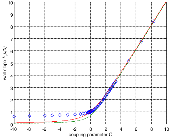
Figure 5: Velocity profile slope at the wall in function of the coupling number: boxes :   boxes : numerical simulation of equation (80), solid line : model (84), dashed line : same as (84) when the velocity profile (82) in the layer is replaced by a straight line.

4.2 Consequences on the global angular momentum - the MAgnetic TURbulence (MATUR) experiment.

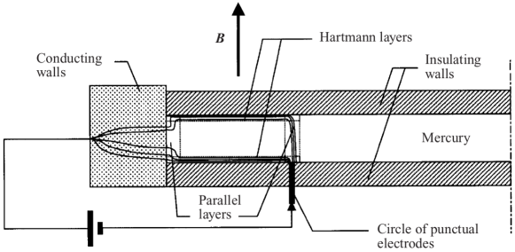
Figure 6: Radial section of Matur experimental setup.

The results of the previous subsection are now compared with experimental results obtained on the device MATUR. The latter is a cylindric container (diameter $0.2m$) with electrically insulating bottom and conducting vertical walls (figure 6). Electric current is injected at the bottom through a large number of point-eclectrodes regularly spread along a circle whose center is on the axis of the cylinder. It is filled with mercury ($1cm$ depth) and the whole device is plunged in a vertical magnetic field. The injected current leaves the fluid through the vertical wall inducing radial electric current lines and gives rise to an azimuthal action on the fluid included in the annulus between the electrode circle and the outer wall. The injected current $j_{W}$ can be considered as a Dirac delta function, centered at the injection radius $r_{e}$, with integral equal to the injected current $I$ : $j_{W}=I/\left(2\pi r_{e}\right)\delta\left(r-r_{e}\right).$ The corresponding  forcing is azimuthal and given from the solution of (12), which yields :

$$\mathbf{v}_{0}\simeq\mathbf{\bar{u}}_{0}=-\dfrac{B}{\rho a}\dfrac{I}{2\pi r}t_{H}.\mathbf{e}_{\theta}.$$ (87)

This annulus of fluid then rotates and gives rise to a concave parallel layer along the outer wall. The upper surface of mercury may be either free or not. But if free, oxidation of mercury makes the upper surface rigid so that a Hartmann layer takes place at the top anyway. Therefore two Hartmann layers (at the top and the bottom) have to be considered ($n=2$ ). A more exhaustive description of the experimental device and results can be found in Alboussière et al. (1999).

The geometry of the fluid motion suggests that an Ekman recirculation occurs, rising up a radial flow toward the parallel wall side layer. One can expect the angular momentum decrease significantly there, altering the behavior of the layer. A good global description of this effect is provided by the balance of the total angular momentum $L=\int r\bar{u}_{\theta}d^{2}\mathbf{r}$. The equation for $L$ can be derived by integration over the whole domain of (76) after multiplication by $r$ (assuming $\mathbf{v\simeq\bar{u}}$) :

$$\dfrac{dL}{dt}=F-S-\dfrac{2L}{t_{H}},$$ (88)

where the global electric forcing $F$ and the viscous dissipation at the wall side layer $S$ take the form :

$$F =\dfrac{IB}{2\rho a}\left(R^{2}-r_{e}^{2}\right),$$ (89)

$$S =2\pi R^{2}\nu\partial_{y}u_{\theta}\rfloor_{wall}$$ (90)

At small forcing, the parallel layer thickness is of order $aHa^{-1/2},$ so the corresponding viscous effect on the angular momentum is negligible in comparison with the Hartmann friction (in a ratio of order $Ha^{1/2}$). Therefore $S$ can be neglected in (88) and

$$F=2\dfrac{L}{t_{H}}$$ (91)

in steady regime. This corresponds to the linear behavior of $L$ versus the forcing current $I$ for moderate $I$ ($I\lesssim 7A$ see figure 7). Notice that the velocity near the wall is then derived from the recirculation $\Gamma,$ by $U=\Gamma/\left(2\pi R\right)$ and it coincides with (87) at $r=R,$ $U=\mathbf{\bar{u}}_{0}\left(R\right).$ Comparing $U$ with $L,$ given from the forcing $F$ by (91), gives

$$L=\pi R\left(R^{2}-r_{e}^{2}\right)U$$ (92)

We observe that the velocity profile remains unchanged even for large currents, so we can use (92) to express the velocity near the wall as a function of $L.$ Introducing this velocity $U$ in the boundary layer model of section 4.1, we can deduce the wall stress $S$. We have found that the asymptotic expression (85) is valid for the considered experimental conditions, allowing a simple expression of $\partial_{y}u_{\theta}\rfloor_{wall}$ in (90). It is then possible to assess every terms in (88) which provides a relation between the injected electrical current and the global angular momentum, which can be compared to experimental results :

$$I=4\dfrac{\sqrt{\sigma\rho\nu}}{R^{2}-r_{e}^{2}}L+\dfrac{7}{18}\dfrac{\sqrt{\nu\rho^{5}\sigma^{-3}}L^{3}}{\left(R^{2}-r_{e}^{2}\right)^{3}\pi^{2}R^{2}B^{4}\alpha^{3}}.$$ (93)

Figures 7 and 8, show experimental measurements of the global angular momentum and theoretical curves. Our model provides a reasonable prediction of the experimental results. This comparison must be put in perspective as MATUR is a very complex device where a wide variety of phenomena occurs. In particular, big vortices are present and break the axisymmetry : firstly, they interact with each other, giving rise to thin shear layers where dissipation occurs, and secondly they interact with the walls, inducing separations in the wall side layers. Furthermore, the Hartmann layer may become turbulent which the present theory does not take in account. Indeed, one can refer to the heuristic criterion established by Hua and Lykoudis (1974)  which states that in rectangular ducts, considerable turbulent fluctuations are observed in the vicinity Hartmann layer for values of $\mathop{\mathrm{R}e}/Ha$ above 250. For $B\geq 0.8T$, the smallest values of this parameter are about $500$. For all these reasons, it is natural that our model predicts a dissipation smaller than observed in the experiment. A numerical simulation of (76) may be able to take unsteadiness into account and to provide better results.

At higher field (figure 8), the saturation has disappeared from experimental measurements, which are then closer to the linear theory curve. This is quite natural as the non linear effects are proportional to $Ha^{-3}$ , which dramatically falls in for increased values of $B.$ Though the experimental points fit a straight line, the latter has not exactly the same slope as the one predicted by the linear theory which is linearly dependent on $1/t_{H}$ . Once again, additional phenomena have to be invoked. Actually, the bottom of the experimental device contains many conducting electrodes in which electric current may pass : in these areas, the damping may be significantly increased, leading to a reduction of the damping time ”felt” by the global angular momentum. This latter phenomenon is certainly responsible for a systematic departure between theory and experiment.

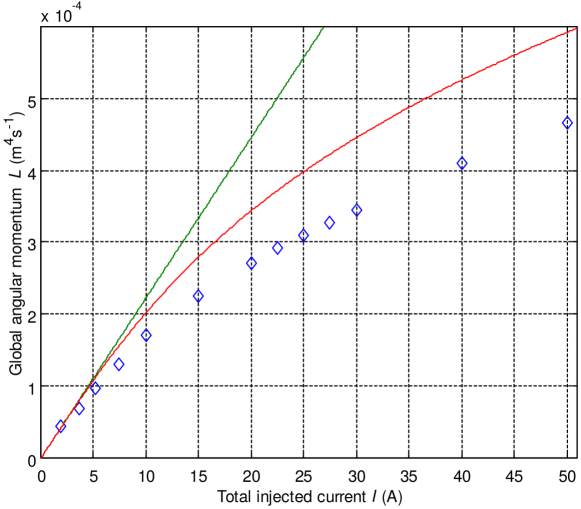
Figure 7: Global Angular momentum in the Matur experimental setup versus total injected electric current for $B=0.17T$ and $r_{e}=93mm$. Dots : experimental measurements, Solid line : theoretical curve for obtained from (93).

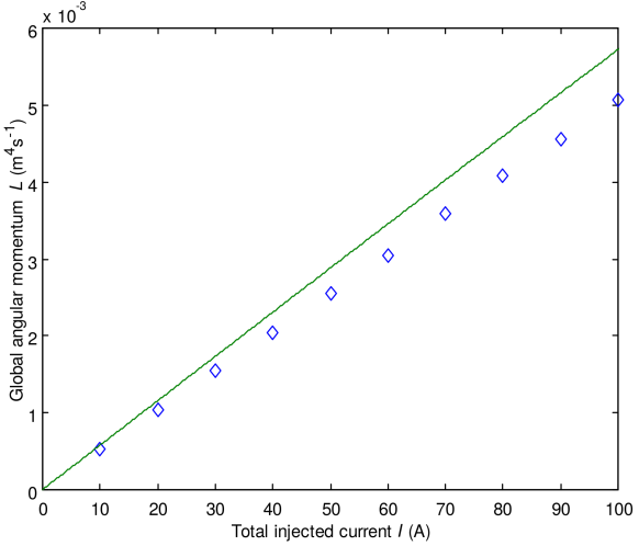
Figure 8: Global Angular momentum in the Matur experimental setup versus total injected electric current for $B=2T$ and $r_{e}=54mm$. Dots : experimental measurements, Solid line : theoretical curve obtained from (93).

4.3 Isolated vortices aroused by a point-electrode. Experimental comparison.

The present subsection is devoted to the improvement of the 2D model of isolated vortices exposed in section 2.2.3. taking in account Ekman recirculation. Indeed, the Sommeria experiments (1988) clearly show that the core of an isolated vortex tends to widen when the injected current is strong. As an Ekman secondary flow is highly suspected of being responsible for this phenomenon, the axisymmetric equation of motion provides a good analytical model for it.

Let us then consider a configuration similar to the one described in paragraph 2.2.3 in which the electric current is injected through a cylindrical electrode of radius (and an upper free surface so that $n=1$) at the center of the vortex, introducing a no-slip condition at this point. We suppose that the forcing satisfies (20). The motion equation (77) has to be rescaled using the scalings of section 2.2.3 $\lambda=\sqrt{Ha}$ and $U=$ $\dfrac{\Gamma}{a}\sqrt{Ha}$. We assume $\mathbf{u}_{0}\simeq\mathbf{v}_{0}$ since $Ha\gg 1$, which leaves the non dimensional equation of motion under the form :

$$C_{t}\dfrac{1}{r^{2}}\partial_{r}\left(rv_{\theta}^{3}\right)=\dfrac{1}{r^{2}}\partial_{r}\left[r^{3}\partial_{r}\left(\dfrac{v_{\theta}}{r}\right)\right]-v_{\theta}+\dfrac{1}{r},$$ (94)

with the corresponding boundary conditions (where $C_{t}=\dfrac{7}{36}\dfrac{\Gamma}{a^{2}}\dfrac{1}{N^{2}}$) :

$$\begin{array}[]{c}v_{\theta}\left(b\right)=0\\ \text{and}\underset{r\rightarrow+\infty}{\lim}v_{\theta}=0,\end{array}$$ (95)

One can also express the non dimensional number $C_{t}$ in function of the local interaction parameter $N_{c}$ introduced by Sommeria (1988) :

$$\begin{array}[]{cc}N_{c}=\dfrac{\sigma B^{2}}{\rho}\dfrac{a^{2}}{\Gamma Ha},&C_{t}=\dfrac{7}{36}\dfrac{1}{N_{c}^{2}}.\end{array}$$ (96)

The latter result, shows that the local interaction parameter is the relevant non-dimensional number which controls the radial profile of azimuthal velocity of the vortex.

For an electrode radius $b=0.1,$ the rod is ten times thinner than the typical parallel layer scale so that this case may be relevantly compared to the experimental case. Indeed, reducing the electrode diameter when the latter is significantly smaller than $1$ do not have any relevant effect on the result. The solutions have been numerically computed thanks to a shooting method featuring a Runge-Kutta algorithm. The radial profile of angular momentum has been processed out from the result . We have computed it for $B=0.5T$ and for two different injected currents ($I=50mA$ and $I=200mA$ respectively corresponding to $C_{t}=8.85$ and $C_{t}=141.65$ ) ; these cases are thus highly non-linear and one can expect the recirculating flow to be significant. The profiles are reported in figure 9 and compared with the experimental results obtained by Sommeria (1988). The radial velocity can be estimated from the continuity equation (3) $u_{r}=\tfrac{5}{6}\tfrac{\lambda}{HaN}\tfrac{\tilde{v}_{\theta}^{2}}{r}$ in non dimensional form, using (1).

The experimental device used by Sommeria is similar to the experiment MATUR except that the electrical current is injected through a single central electrode and the upper surface is free (see figure 10 and 11.). The velocity measurements are obtained thanks to a visualization technique including streak photos of particles in the fluid. The numerical simulations performed using our non linear model gives a good agreement with the experimental results : it turns out that the vortex core actually broadens for higher values of the electric current, i.e. for highest values of $C_{t}$). This is due to a radial flow resulting from inertial effects. Indeed, in axisymmetric configuration, the vertical flow $w^{-}$ (63) is proportional to $1/r\partial_{r}\left(u_{\theta}^{2}/r\right)$ so that a strong flow rate from the Hartmann layer occurs at the center of the vortex. This flow softly closes at large $r$ , which is analogous to the traditional Ekman pumping.

To quantify this phenomenon of spreading vortices, we have plotted the radius $R_{v}$ of the vortex obtained from the numerical simulations of (94) versus the value of the core related interaction parameter $N_{c}$.The results are plotted in figure 12 and it appears that $R_{v}\sim N_{c}^{-1}$. This scaling law is in agreement with experimental measurements of Sommeria (1988). However, a quantitative comparison of the prefactor is difficult because the experimental results are derived from electric potential measurements which are sensitive to the singularity at the electrode.

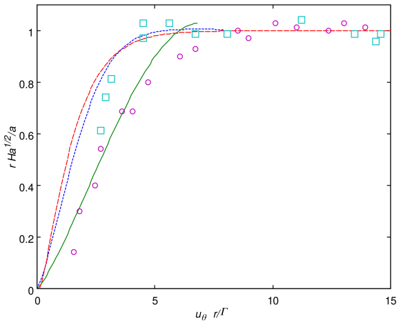
Figure 9: Vortex radial profile of angular momentum for $B=0.5T$ : boxes : experimental measurements for injected current $I=0.05A,$ circles : experimental measurements for $I=0.2A,$ full line : analytical profile without non linear effects, semi dotted line : numerical profile for $I=0.05A$, dotted line : numerical profile for $I=0.2A$. Note that numerical precision problems don’t allow to get to profiles for any values of r.

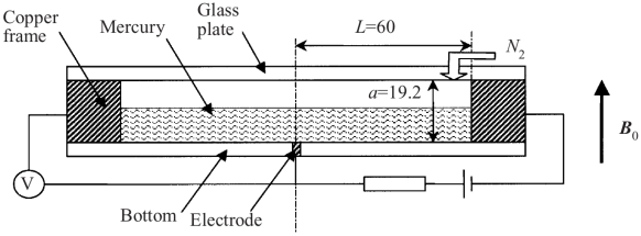
Figure 10: Experimental device of Sommeria’s vortex study : cross section of the circular tank with a shematic representation of the current supply and device for potential measurement. Dimensions are indicated in mm.

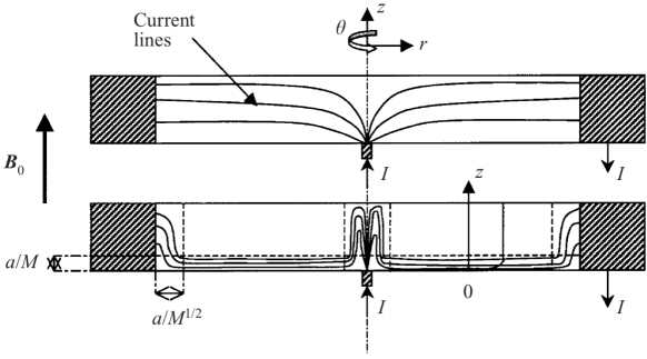
Figure 11: The electric current streamlines (a) without Magnetic field (b) in a strong magnetic field. The Hartmann layer, the outer layer parallel to the field and the vortex core are represented, as well as a vertical velocity profile.

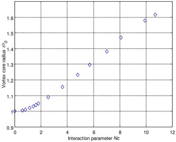
Figure 12: Vortex core radius normalized by its value without non-linear effect $r_{0}$(corresponding to very low injected electric current) versus the inverted core interaction parameter. The results are obtained from numerical simulations of equation (94).

5 Conclusion.

Our analysis applies for flows in ducts with transverse uniform magnetic field, a standard configuration of interest in various MHD problems. These flows often involve complex 3D velocity fields, with both transverse structures and vertical variations in the thin Hartmann boundary layer. The latter is very difficult to resolve numerically at high Hartmann number, due to the high spatial resolution required. Our effective 2D model provides thus a great  simplification.

This model has been derived by a systematic expansion in terms of the two small parameters $1/N$ and $1/Ha$ providing  a good understanding of its range of validity. At zero order, we recover the 2D core model of Sommeria & Moreau (1982) which is already a good approximation even in parallel layers near lateral walls or around a central electrode scaling like $Ha^{-1/2}$ (as seen in section 2).

The expansion is valid for sufficiently large transverse scales $\lambda$. In principle $\lambda<Ha^{-1/2}$ has to be satisfied, but the zero order solution turns out to provide good results even in parallel layers, of thickness of order $Ha^{-1/2}$. Perturbations at the scale of order $Ha^{-1}$can arise in the Hartmann layer, when it becomes unstable. This is experimentally observed for $\dfrac{N}{Ha}>250$. Such a small scale effect is not captured by our expansion.

A first correction to the 2D core model occurs as weakly three-dimensional velocity profiles parabolic in $z$ at first order. This effect can be interpreted as the consequence of the finite diffusion time of momentum by electromagnetic effects. This diffusion leads to complete two-dimensionality only in the limit of very large magnetic field ($Ha\rightarrow\infty$). Vortices look like ”barrels” instead of columns. We however find that this essentially linear effect has little influence on the global dynamics, involving $z$-averaged quantities.

The second perturbation corresponds to Ekman recirculation effects within the Hartmann boundary layers. This recirculation transports momentum, which significantly modifies the dynamics of the $z$-averaged velocity. These recirculating effects can also have interesting consequences for the transport of heat or chemicals away from the Hartmann layers.

Analytical solutions of our effective 2D model in axisymmetric configurations appear in reasonable agreement with laboratory experiments. The model explains the additional dissipation of angular momentum due to radial transport by recirculation. For the experiments of Sommeria (1988), it explains the spreading of vortex core and fits the experimental law in $N^{-1}.$

Finally, it is noteworthy that recirculation effects lead to new scaling laws for side layers along concave or convex walls parallel to the magnetic field. Along a convex wall, the side layer is widened according to equation (80) whose numerical solution is plotted in figure 5. Along a concave wall, on the contrary, it becomes thinner and the scaling law is in $NHa^{-1}$.

References

T.ALBOUSSIERE, V.USPENSKI & R.MOREAU 1999 Quasi-2D MHD Turbulent Shear Layers Experimental thermal and Fluid Science 20 pp19-24.

A.ALEMANY, R.MOREAU, P.SULEM & U.FRISCH 1979 Influence of an External Magnetic Field on Homogeneous MHD Turbulence Journal de Mecanique 18(2) pp 277-313.

L. BÜHLER 1996 Instabilities in Quasi Two-Dimensional Magnetohydrodynamic Flows J. Fluid. Mech 326 125-150.

P.A.DAVIDSON 1997 The Role of Angular Momentum in the Magnetic Damping of Turbulence J. Fluid. Mech. 336 123-150.

H.M.HUA & P.H.LYKOUDIS 1974 Turbulent Measurements in Magneto-Fluid Mechanics Channel Nucl. Sci. Eng.45 445.

J.C.R. HUNT & W.E. WILLIAMS 1968 Some Electrically Driven Flows in Magnetohydrodynamics. Part 1. Theory.J. Fluid. Mech. 31(4) 705-722.

J.C.R.HUNT & S.SHERCLIFF 1971 Magnetohydrodynamics at High Hartmann Number Ann. Rev. Fluid. Mech. 3 37-62.

A.B.TSINOBER & Y.B.KOLESNIKOV 1974 Experimental Investigation of Two-Dimensional Turbulence Behind a Grid Isv. Akad. Nauk. SSSR Mech. Zhod. i Gaza 4 146.

O.LIELAUSIS 1975 Liquid Metal Magnetohydrodynamics Atomic Energy Review 13 527.

R.MOREAU 1990 Magnetohydrodynamics Kluwer Academic Publishers

R. MOREAU 1998 Applied Scientific Research Magnetohydrodynamics at the Laboratory Scale : Established Ideas and New Challenges 58 131-147

P.H.ROBERTS 1967 Introduction to Magnetohydrodynamics Longmans.

S. SHERCLIFF 1953 Proc. Camb. Phil. Soc.49 136.

J.SOMMERIA & R.MOREAU 1982 Why, How and When MHD Turbulence Becomes Two-Dimensional J. Fluid. Mech. 118 507-518.

J.SOMMERIA 1988 Electrically Driven Vortices in a Strong Magnetic Field J. Fluid. Mech 189 553-569.

O.ZIGANOV & A.THESS 1998 Direct Numerical Simulations of Forced MHD Turbulence at Low Magnetic Reynolds Number J. Fluid. Mech. 358 299-333.

M.I LOFFREDO 1986 Extension of Von Karman Ansatz to Magnetohydrodynamics Mecanica 21 81-86.

H.G.LUGT 1996 Introduction to Vortex Theory potamac Maryland.

R.S.NANDA & H.K. MOHANTY 1970 Hydrodynamic Flow in Rotating Channel Appl. Sci. Res. 24 65-78.

B.MÜCK, C.GÜNTHER, U.MÜLLER & L.BÜHLER 2000 Three-Dimensional MHD Flows in Rectangular Ducts with Internal Obstacles.submitted to J. Fluid. Mech.